Improving Simulations with Symmetry
Control Neural Networks

Abstract

The dynamics of physical systems is often constrained to lower dimensional sub-spaces due to the presence of conserved quantities. Here we propose a method to learn and exploit such symmetry constraints building upon Hamiltonian Neural Networks. By enforcing cyclic coordinates with appropriate loss functions, we find that we can achieve improved accuracy on simple classical dynamics tasks. By fitting analytic formulae to the latent variables in our network we recover that our networks are utilizing conserved quantities such as (angular) momentum.

1 Introduction

For accurate simulations, building in a bias to deep neural networks has been a key mechanism to achieve extra-ordinary performance. An example for such a bias is to learn a motion which is conserving energy as performed in the context of Hamiltonian Neural Networks (HNNs) (Greydanus et al., 2019). More generally speaking, possible dynamics are constrained due to symmetries of the system and they take place on a sub-space of available phase space (e.g. surfaces of constant energy and total angular momentum). Whereas energy has been built into the functional biasing of neural networks, further symmetries are at this moment enforced by hand which requires domain knowledge of the system. Here we describe a method on how to automatically search for and use such symmetries in neural networks used for simulations. In addition this method turns out to reveal – at this stage for simple systems – analytic expressions for the conserved quantities. Our method is based on enforcing the network to perform canonical coordinate transformations in a first network $T_{\psi}$ which enforces some of the latent coordinates to become constant (cyclic coordinates in the language of Hamiltonian dynamics). From these new coordinates the network then predicts the Hamiltonian underlying the dynamics of this system with a second network $H_{\phi}.$ The structure of our networks – to be described more accurately later on – can be found in Figure 1.

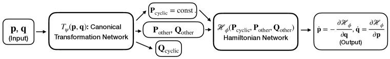
Figure 1: Structure of symmetry control networks: The network $T_{\psi}$ transforms the input coordinates of phase space $({\bf p},{\bf q})$ to canonical coordinates where some coordinates are forced to be cyclic. These coordinates are used as input to the Hamiltonian network $H_{\phi}$. The output, the time derivatives of our initial coordinates, is calculated from the Hamiltonian using auto-differentiation.

We demonstrate in our experiments that multiple conserved quantities can indeed be automatically identified with this method, we find improvements in the predictions of our dynamics in comparison with HNNs, and we can find analytic expressions for the conserved quantities.

2 Theory

When motion is taking place on a sub-space of phase space, one can reduce the number of coordinates describing the system. Every independent conserved quantity reduces the number of coordinates needed to describe a system until all coordinates are constrained (integrable systems). Even though we do not know apriori the conserved coordinates, Hamiltonian mechanics provides general conditions for such coordinates. In particular the time derivative of any function on phase space, described by positions ${\bf q}$ and momenta ${\bf p}$ of our $N$ particles in $d$ spatial dimensions, is given by

$$\frac{dg(\bf{q},\bf{p})}{dt}=\sum_{i=1}^{N\cdot d}\frac{\partial g}{\partial q_{i}}\frac{dq_{i}}{dt}+\frac{\partial g}{\partial p_{i}}\frac{dp_{i}}{dt}=\{g,\mathcal{H}\}\leavevmode\nobreak\ .$$ (1)

In the last step we have used the Poisson brackets and Hamilton’s equations which are given as:

$$\{f,g\}:=\sum_{i=1}^{N\cdot d}\frac{\partial f}{\partial q_{i}}\frac{\partial g}{\partial p_{i}}-\frac{\partial f}{\partial p_{i}}\frac{\partial g}{\partial q_{i}}\,,\qquad\frac{d\bf{q}}{dt}=\frac{\partial\mathcal{H}}{d\bf{p}}=\{{\bf q},\mathcal{H}\}\,,\qquad\frac{d{\bf p}}{dt}=-\frac{\partial\mathcal{H}}{d\bf{q}}=\{\bf{p},\mathcal{H}\}\,.$$ (2)

Here we are interested in enforcing coordinate transformations $T$ which enforce that at least one of the new momenta ${\bf P}$ is conserved

$$0=\dot{P}_{i}=-\frac{\partial\mathcal{H}}{\partial Q_{i}}=\{P_{i},\mathcal{H}\}\,.$$ (3)

We are interested in a particular type of coordinate transformations, namely canonical transformations which are which are transformations that leave the structure of the Hamiltonian equations (2) and in particular the Poisson bracket unchanged (allowing for the evaluation with respect to the input variables):

$$T:\left({\bf q},{\bf p}\right)\mapsto\left({\bf Q}({\bf q},{\bf p}),{\bf P}({\bf q},{\bf p})\right),$$

$$\{f,g\}_{{\bf p},{\bf q}}=\{f,g\}_{{\bf P},{\bf Q}}\leavevmode\nobreak\ ,\;\;\;\mathcal{H}({\bf p},{\bf q})=\tilde{\mathcal{H}}({\bf P}({\bf p},{\bf q}),{\bf Q}({\bf p},{\bf q}))\leavevmode\nobreak\ .$$ (4)

We enforce this conservation by adding an appropriate loss term corresponding to the condition in (3). When such a constraint is enforced, the Hamiltonian does not depend on the associated $Q_{i},$ i.e. it depends on fewer degrees of freedom and the motion in phase space is restricted to a lower dimensional manifold. Put differently, the cyclic coordinates provide via constraints of the type (3) additional restrictions on the allowed Hamiltonian function which we learn with our symmetry control neural networks.(cf. Figure LABEL:fig:losscontours shows the explicit constraint from angular momentum conservation in a 2-body example in addition to constraints arising from satisfying the Hamiltonian equations of motion).

These conditions lead to two additional loss components in addition to the standard HNN-loss:

1. The first loss ensures that our Hamiltonian satisfies Hamiltonian equations (2), which we can ensure as follows:

   $$\mathcal{L}_{\rm HNN}=\sum_{i=1}^{N\cdot d}\left\lVert\frac{\partial\mathcal{H}_{\phi}({\bf P},{\bf Q})}{\partial p_{i}}-\frac{dq_{i}}{dt}\right\rVert_{2}+\left\lVert\frac{\partial\mathcal{H}_{\phi}({\bf P},{\bf Q})}{\partial q_{i}}+\frac{dp_{i}}{dt}\right\rVert_{2}\,.$$ (5)

   The time derivatives are provided by the data and the derivatives of the Hamiltonian with respect to the input variables can be obtained using auto-differentiation. This is the same loss as introduced in Greydanus et al. (2019).

2. To ensure that our transformation $T_{\psi}$ are of the type we are interested in (cf. Eq. (4)), i.e. our new coordinates fulfil the Poisson algebra, we enforce the following loss:

   $$\mathcal{L}_{\rm Poisson}=\sum_{i,j=1}^{N\cdot d}\left\lVert\{Q_{i},P_{j}\}-\delta_{ij}\right\rVert_{2}+\sum_{i,j>i}^{N\cdot d}\left\lVert\{P_{i},P_{j}\}\right\rVert_{2}+\left\lVert\{Q_{i},Q_{j}\}\right\rVert_{2}\leavevmode\nobreak\ ,$$ (6)

   where in some practical applications we only enforce this loss on $n$ cyclic coordinate pairs. The first part of this loss ensures that a vanishing solution is not allowed.

3. Hamilton’s equations have still to be satisfied with respect to the new coordinates. For the cyclic coordinates we have enforced by our architecture that ${\cal H}_{\rm\phi}$ is independent of $Q_{i}.$ To ensure that $P_{i}$ is actually conserved, we require the following additional loss:

   $$\mathcal{L}_{\rm HQP}^{(n)}= \sum_{i=1}^{n}\left\lVert{\displaystyle\frac{dP_{i}}{dt}}\right\rVert_{2}\!+\!\left\lVert\frac{dQ_{i}}{dt}-\frac{\partial\mathcal{H}_{\phi}({\bf P},{\bf Q})}{\partial P_{i}}\right\rVert_{2}$$

   $${+\beta\sum_{i=n+1}^{N\cdot d}\left\lVert\frac{dP_{i}}{dt}+\frac{\partial\mathcal{H}_{\phi}({\bf P},{\bf Q})}{\partial Q_{i}}\right\rVert_{2}+\left\lVert\frac{dQ_{i}}{dt}-\frac{\partial\mathcal{H}_{\phi}({\bf P},{\bf Q})}{\partial P_{i}}\right\rVert_{2}\leavevmode\nobreak\ ,}$$ (7)

   where $n$ denotes the number of cyclic variables we are imposing and $\beta$ denotes a hyperparameter. For our networks we only constrain the cyclic coordinates and use $\beta=0$. The time derivatives can be calculated using either expressions in (1).

Our total loss is a weighted sum of these three components:

$${\cal L}=\mathcal{L}_{\rm HNN}+\alpha_{1}\mathcal{L}_{\rm Poisson}+\alpha_{2}\mathcal{L}_{\rm HQP}^{(n)}\leavevmode\nobreak\ ,$$ (8)

where the weights $\alpha_{i}$ are tuned.

For integrating the solutions in time from our respective symmetry control network we use a fourth order Runge-Kutta integrator as in Greydanus et al. (2019) which unlike symplectic integrators allows for a comparison with neural network approaches directly predicting the dynamics of a system.

Regarding the efficiency of this approach, there is no additional cost during the inference procedure. During training our loss requires the additional evaluation of already calculated gradients. The number of these terms scales cubically with the product of number of dimensions and particles $(N\cdot d)^{3}$ (cf. Poisson loss). This cost is lowered when the conserved quantities are known (e.g. from prior knowledge of the system) as the Poisson loss is automatically satisfied and we only invoke an additional loss contribution on the Hamiltonian for each conserved quantity. We note that for cases where the Hamiltonian involves only local interactions an evaluation of these constraints on these local interactions is relevant which results in a reduction of the relevant additional loss terms to the respective local terms, significantly reducing the calculational cost. Hence the cost is not significantly enhanced compared to the HNN case.

3 Experiments

Our experiments are designed with the following goals in mind:

1. SCNN: We want to compare the performance of symmetry control neural networks with HNNs and baseline neural networks which directly predict $(\dot{\bf q},\dot{\bf p})$. We want to take advantage of unknown underlying symmetries while we do not have any domain knowledge of our system. The main hyperparameter is the number of conserved quantities.

2. SCNN-constraint: We explore whether imposing domain knowledge about symmetries improves the performance. This is motivated by the fact that we often know about the existence of certain conserved quantities such as (angular) momentum.

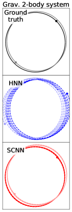
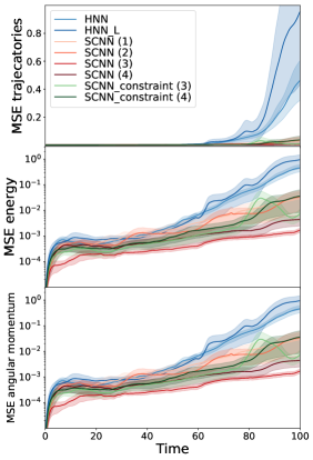
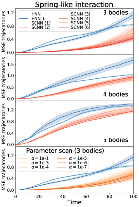
Figure 2: Comparison between two HNN networks as described in the main text and SCNN networks with different numbers of conserved quantities. Left: Sample trajectories of the gravitational two-body problem. Middle: Comparison of the mean-squared deviation of the trajectories, the conservation of energy and angular momentum for the 2-body problem. Right: Comparison of the mean-squared deviations for various spring-like interactions. The bottom plot shows the well-behaved dependence on the loss prefactor $\alpha=\alpha_{i}.$ For all evaluations of the trajectories we show the mean and single standard deviation over $10$ different initializations evaluated on $100$ trajectories. $\alpha_{1}=\alpha_{2}=10^{-n}$ where $n$ is the number of constraint conserved quantities.

We test these architectures on several different physical systems: the gravitational two-body problem, an $n$-body system with spring-like interactions, an electrically charged particle in a magnetic field, a spherical pendulum, and a double pendulum. We describe the hyperparameter dependence of our architecture on the former two in more detail and report only the results of our hyperparameter scan for the latter three. The spring-like interaction contained between 3 and 5 particles each interacting with the force ${\bf F^{ij}}=-k\leavevmode\nobreak\ \left({\bf x}^{i}-{\bf x}^{j}\right)$. The gravitational force is described by ${\bf F^{ij}}=-k\leavevmode\nobreak\ \frac{({\bf x}^{i}-{\bf x}^{j})}{|{\bf x}^{i}-{\bf x}^{j}|^{3}}$.

To understand the effect of the number of conserved quantities and the loss prefactors $\alpha_{i}$, we performed a parameter scan for the number of conserved quantities and these prefactors. To compare the precision of the networks we computed the particle trajectories of $100$ different system initializations and compared them to the ground truth over $100$ timesteps. In addition, we check the conservation of energy and angular momentum for the gravitational 2-body problem. Our networks are trained on datapoints corresponding to the first $50$ timesteps which allows us to compare the generalization of our networks on unseen regions of phase-space. The results are summarized in Figure 2. Overall, these results show that the SCNN learns a much more stable and accurate Hamiltonian and we find that the SCNN-constraint networks are not able to outperform the SCNN networks. The baseline network is omitted from these plots as its performance is significantly worse. The HNN network has the same complexity as our ${\cal H}_{\phi}$ network with two dense layers and the HNN_L network corresponds to a complexity of five dense layers, i.e. the combined complexity of our $T_{\psi}$ and ${\cal H}_{\phi}$ network. The loss prefactor dependence is such that the more conserved quantities we use, the smaller the prefactors have to be which is due to the increase in loss terms contributing.

In the setup with a charged particle in a magnetic field, a spherical pendulum, and the double pendulum the improved performance of our SCNN(-constraint) networks compared to HNN is confirmed. Table 1 shows the mean-squared error predictions which we obtain after $100$ timesteps. A description of these systems can be found in Appendix A.

Experiment	SCNN	SCNN-constraint	HNN
Magnetic field	$0.164\pm 0.025$	${\bf 0.033\pm 0.010}$	$0.083\pm 0.019$
Spherical pendulum	$0.092\pm 0.33$	${\bf 0.055\pm 0.005}$	$0.288\pm 0.007$
Double pendulum	${\bf 0.014\pm 0.004}$	–	$0.117\pm 0.012$

Table 1: The MSE after 100 time steps for different experiments. For the double pendulum we compare the MSE after 20 time steps. The data points are collected for 10 different initalizations and the error bars correspond to single standard deviation. All SCNN networks in these experiments have two conserved quantities. The best performing approach is highlighted.

Search for conserved quantities

The conserved quantities of our SCNN networks can be analysed by fitting a low-dimensional polynomial ansatz to the respective network predictions. This reveals that our SCNN finds the angular momentum and the total momentum as conserved quantities in the gravitational two-body system:

$$\begin{split}P_{c_{1}}=&-4.2\leavevmode\nobreak\ p_{x_{1}}-4.2\leavevmode\nobreak\ p_{x_{2}}-1.3\leavevmode\nobreak\ p_{y_{1}}-1.3\leavevmode\nobreak\ p_{y_{2}}\leavevmode\nobreak\ ,\\ P_{c_{2}}=&-0.9\leavevmode\nobreak\ p_{x_{1}}-0.9\leavevmode\nobreak\ p_{x_{2}}-3.2\leavevmode\nobreak\ p_{y_{1}}-3.2\leavevmode\nobreak\ p_{y_{2}}\leavevmode\nobreak\ ,\\ L=&\leavevmode\nobreak\ 1.0\leavevmode\nobreak\ q_{x_{1}}p_{y_{1}}+0.9\leavevmode\nobreak\ q_{x_{1}}p_{y_{2}}+0.9\leavevmode\nobreak\ q_{x_{2}}p_{y_{1}}-1.0\leavevmode\nobreak\ q_{x_{2}}p_{y_{2}}\\ &+1.0\leavevmode\nobreak\ q_{y_{1}}p_{x_{1}}-0.9\leavevmode\nobreak\ q_{y_{1}}p_{x_{2}}-0.9\leavevmode\nobreak\ q_{y_{2}}p_{x_{1}}+1.0\leavevmode\nobreak\ q_{y_{2}}p_{x_{2}}\leavevmode\nobreak\ .\end{split}$$ (9)

For more sophisticated conserved quantities (i.e. non-polynomial conserved quantities) different ansätze seem necessary (some of which are pursued in related work (Sahoo et al., 2018; Cranmer et al., 2019; Wetzel et al., 2020).

4 Outlook and related work

Our SCNNs naturally connect with work on inferring dynamics with neural networks such as (Battaglia et al., 2016) in the same way as HNNs. Natural extensions of our current work can include the application on graph neural network based approaches (Sanchez-Gonzalez et al., 2019) and in flows (Toth et al., 2020). With respect to applications, we particularly look forward to applying our new approach for automatically inferring and using the symmetries in astrophysical and molecular dynamics settings.

Appendix A Details on further physical systems

Here we describe the additional three physical systems which we used in our experiments.

A.1 Spherical Pendulum

The spherical pendulum is governed by the following Hamiltonian:

$$\mathcal{H}=\frac{p_{x}^{2}+p_{y}^{2}}{2m}-m\leavevmode\nobreak\ g\leavevmode\nobreak\ \sqrt{l^{2}-q_{x}^{2}-q_{y}^{2}}\leavevmode\nobreak\ ,$$ (10)

where we take a universal mass $m=\frac{1}{2}$ coupling $g=\frac{1}{2}$ and pendulum length $l=1$. In this system, the angular momentum in z-direction is conserved:

$$L=q_{x}p_{y}-q_{y}p_{x}\leavevmode\nobreak\ .$$ (11)

We sample the starting conditions $\left(\bf{q}\left(t=0\right),\bf{p}\left(t=0\right)\right)$ from a uniform distribution from the interval $(-1,1)$. We ensure, that the energy is well-defined and negative.

For our dataset we utilise 100 initial conditions and generate 500 points on the trajectory. These points are take from a time span of 20 which corresponds to a time where multiple periodic motions are included. We use a 80:20 split for the training and test set.

A.2 Charged particle in a magnetic field

The charged particle in a magnetic field, where we choose a circular B-field plus an electric field, is governed by the following Hamiltonian:

$$\mathcal{H}=\frac{1}{2m}\left(\left(p_{x}+q\leavevmode\nobreak\ q_{y}\leavevmode\nobreak\ B\right)^{2}+\left(p_{y}-q\leavevmode\nobreak\ q_{x}\leavevmode\nobreak\ B\right)^{2}\right)+k\leavevmode\nobreak\ \left(q_{x}^{2}+q_{y}^{2}\right)\leavevmode\nobreak\ ,$$ (12)

where we take a universal mass $m=\frac{1}{2}$, electric field $k=1$, charge $q=1$ and B-field $B=1$. Again angular momentum is conserved. We sample the starting conditions $\left(\bf{q}\left(t=0\right),\bf{p}\left(t=0\right)\right)$ from a uniform distribution from the interval $(-1,1)$, We then normalize the vector to unit length and then re-scale it uniformly to a vector of length in the interval $(0.1,1.0).$ For our dataset we utilise 100 initial conditions and generate 500 points on the trajectory. These points are take from a time span of 20 which corresponds to a time where multiple periodic motions are included. We use a 80:20 split for the training and test set.

A.3 Double pendulum

The double pendulum can be described by the following Hamiltonian:

$$\mathcal{H}= \leavevmode\nobreak\ \frac{l_{2}^{2}m_{2}p_{2}^{2}+l_{1}^{2}(m_{1}+m_{2})p_{2}^{2}-2m_{2}l_{1}l_{2}p_{1}p_{2}\cos{\left(\theta_{1}-\theta_{2}\right)}}{2l_{1}^{2}l_{2}^{2}m_{2}\left(m_{1}+m_{2}\sin^{2}{(\theta_{1}-\theta_{2})}\right)}$$

$$-(m_{1}+m_{2})gl_{1}\cos{\theta_{1}}-m_{2}gl_{2}\cos{\theta_{2}}\leavevmode\nobreak\ ,$$ (13)

where we set all scales to unity, i.e. $m_{1}=m_{2}=l_{1}=l_{2}=g=1.$ We sample the starting conditions $\left(\bf{q}\left(t=0\right),\bf{p}\left(t=0\right)=0\right)$ from a uniform distribution from the interval $(0,2\pi)$. Note, that $\theta_{1}$ and $\theta_{2}$ are angles and therefore, we have to ensure that they always lie in the interval $(0,2\pi)$. For our dataset we utilise 100 initial conditions and generate 500 points on the trajectory. These points are take from a time span of 20 which corresponds to a time where multiple periodic motions are included. We use a 80:20 split for the training and test set.

Appendix B Hyperparameters

We have performed some hyperparameter searches for our symmetry control networks on which we give an overview here.

By varying the hidden layer size between 50-300, we find that there is a minimum size of layer size $200$ to find convergence of our networks. We have varied the number of hidden layers up to $5$ hidden layers. Two hidden layers are already sufficient (tested up to 5 hidden layers), hence we restricted ourselves on them. Coarsely speaking, we find that the precise architecture is less relevant in our current experiments.

More relevant are the pre-factors in the loss. Depending on the choice, we can either force our networks for better performance on the predictions or obtaining the conserved quantities. We have used $\alpha_{i}$ in the range $[10^{-7},1].$ For this trade-off, we have optimized the experiments in this paper on the particle trajectories.

We find that pytorch’s standard orthogonal initialization provides the best results out of the standard initializations. We have not observed a large random seed dependence.

As datasets we use the nearly circular orbits constructed by Greydanus et al. (2019), but give the whole system a boost in a random direction sampled from $\mathcal{N}\left(0,0.1\right)^{2}$. For the spring-like interaction, we initialize the first $n-1$ particles with $\left(\mathbf{q},\mathbf{p}\right)$ from $\mathcal{U}\left(\left[-1.5,1.5\right]\right)^{4}$. For the $n$-th particle, we use $\left(\mathbf{q},\mathbf{p}\right)=\left(\sum_{i}\mathbf{q}_{i},\sum_{i}\mathbf{p}_{i}\right)$, which ensures that the center of mass is at rest.

References

- Battaglia et al. (2016) Peter Battaglia, Razvan Pascanu, Matthew Lai, Danilo Jimenez Rezende, et al. Interaction networks for learning about objects, relations and physics. In Advances in neural information processing systems, pp. 4502–4510, 2016.
- Cranmer et al. (2019) Miles D Cranmer, Rui Xu, Peter Battaglia, and Shirley Ho. Learning symbolic physics with graph networks. arXiv preprint arXiv:1909.05862, 2019.
- Greydanus et al. (2019) Sam Greydanus, Misko Dzamba, and Jason Yosinski. Hamiltonian neural networks. CoRR, abs/1906.01563, 2019. URL http://arxiv.org/abs/1906.01563.
- Rein & Liu (2012) H. Rein and S. F. Liu. REBOUND: an open-source multi-purpose N-body code for collisional dynamics. AAP, 537:A128, January 2012. doi: 10.1051/0004-6361/201118085.
- Sahoo et al. (2018) Subham Sahoo, Christoph Lampert, and Georg Martius. Learning equations for extrapolation and control. In Jennifer Dy and Andreas Krause (eds.), Proceedings of the 35th International Conference on Machine Learning, volume 80 of Proceedings of Machine Learning Research, pp. 4442–4450, Stockholmsmässan, Stockholm Sweden, 10–15 Jul 2018. PMLR. URL http://proceedings.mlr.press/v80/sahoo18a.html.
- Sanchez-Gonzalez et al. (2019) Alvaro Sanchez-Gonzalez, Victor Bapst, Kyle Cranmer, and Peter Battaglia. Hamiltonian graph networks with ode integrators. arXiv preprint arXiv:1909.12790, 2019.
- Toth et al. (2020) Peter Toth, Danilo J. Rezende, Andrew Jaegle, Sébastien Racanière, Aleksandar Botev, and Irina Higgins. Hamiltonian generative networks. In International Conference on Learning Representations, 2020. URL https://openreview.net/forum?id=HJenn6VFvB.
- Wetzel et al. (2020) Sebastian J. Wetzel, Roger G. Melko, Joseph Scott, Maysum Panju, and Vijay Ganesh. Discovering symmetry invariants and conserved quantities by interpreting siamese neural networks, 2020.