Fourth- and fifth-order virial expansion of harmonically trapped fermions at unitarity

Abstract

By generalizing our automated algebra approach from homogeneous space to harmonically trapped systems, we have calculated the fourth- and fifth-order virial coefficients of universal spin-$1/2$ fermions in the unitary limit, confined in an isotropic harmonic potential. We present results for said coefficients as a function of trapping frequency (or, equivalently, temperature), which compare favorably with previous Monte Carlo calculations (available only at fourth order) as well as with our previous estimates in the untrapped limit (high temperature, low frequency). We use our estimates of the virial expansion, together with resummation techniques, to calculate the compressibility and spin susceptibility.

Introduction.- At low enough temperatures, or high enough densities, matter invariably displays its quantum mechanical nature, first and foremost by virtue of quantum statistics (i.e. particles are ultimately bosonic or fermionic, at least in three spatial dimensions) but also due to interaction effects that may alter the nature of the equilibrium state. As the temperature is raised, these systems eventually undergo a quantum-classical crossover (QCC) in which interactions still play a role, but where quantum mechanical effects are slowly washed out by temperature fluctuations. This regime is especially interesting for strongly coupled matter, in particular in cases where a superfluid phase is present, as the behavior above the superfluid critical temperature (i.e. in the un-ordered phase) is still significantly affected by the interactions (e.g. inducing pairing correlations) but there are no obvious effective theory descriptions [1, 2, 3, 4, 5, 6, 7, 8, 9, 10].

The QCC is governed by the so-called virial expansion (VE) [11], which breaks the quantum many-body problem into $n$-particle subspaces, captured in the so-called virial coefficients (see Ref. [12] for a review). For bulk thermodynamic quantities the virial coefficients are denoted by $b_{n}$, and their change due to interactions is $\Delta b_{n}$. The calculation of $\Delta b_{n}$ has a sparse history that started with $\Delta b_{2}$ in 1937, by Beth and Uhlenbeck [13] and remained largely quiet until the early 21st century. On the theory side, this quiet period can be attributed to the well-known fact that the quantum two-body problem is considerably easier to solve (and to relate to two-body scattering properties) than its three- and higher-body counterparts. On the experimental side, these quantum virial coefficients became increasingly relevant in the early 2000’s with the rise of ultracold atom experiments around the world and their ever-increasing ability to create, manipulate, and measure atomic clouds [14].

One of the most famous systems studied with ultracold atoms is the so-called unitary limit of the spin-$1/2$ Fermi gas [15], which represents a universal regime relevant for atomic and nuclear physics [16, 17, 18, 19, 20, 21]. In this work we investigate the QCC of this universal regime using the VE up to fifth order for a system confined by a harmonic oscillator (HO) potential. Previous numerical work calculated $\Delta b_{3}$ [22, 23, 24, 25, 26, 27] and $\Delta b_{4}$ [28, 29, 30, 31] (see also Ref. [32, 33, 34]). More recent work [35] studied analytic expressions in the so-called semiclassical approximation (previously implemented in a wide variety of situations [36, 37, 38, 39, 40, 41]), which uses a coarse discretization of imaginary time. On the experimental side, there have also been attempts to determine $\Delta b_{4}$ at unitarity in the untrapped limit, using measurements of the equation of state [42, 43], However, those analyses are numerically challenging because one must fit a fourth-order polynomial assuming higher-order contributions are small (which is not necessarily the case, as shown in Ref. [40]).

In this work we generalize the above calculations to include $\Delta b_{5}$ and go far beyond the semiclassical approximation, extrapolating to the continuous imaginary time limit. While we restrict ourselves to the unitary limit for the most part, we provide approximate analytic formulas that apply to arbitrary interaction strengths, trap frequency, and spatial dimension.

Hamiltonian and virial expansion.- In this work we focus on a system of harmonically trapped spin-$1/2$ fermions interacting via a short-range interaction. Thus, the Hamiltonian is $\hat{H}=\hat{T}+\hat{V}_{\text{ext}}+\hat{V}$, where

$$\hat{T}=\sum_{s=\uparrow,\downarrow}\int d^{3}r\leavevmode\nobreak\ \hat{\psi}_{s}^{\dagger}(\mathbf{r})\left(-\frac{\hbar\nabla^{2}}{2m}\right)\hat{\psi}_{s}(\mathbf{r}),$$ (1)

is the kinetic energy operator,

$$\hat{V}_{\text{ext}}=\int\!d^{3}r\,\frac{1}{2}m\omega^{2}{\bf r}^{2}\left[\hat{n}_{\uparrow}({\bf r})+\hat{n}_{\downarrow}({\bf r})\right],$$ (2)

is the external potential energy operator, and

$$\hat{V}=-g\int d^{3}r\leavevmode\nobreak\ \hat{n}_{\uparrow}(\mathbf{r})\hat{n}_{\downarrow}(\mathbf{r}),$$ (3)

is the interaction. Above, $m$ is the mass of the particles, $\omega$ is the isotropic harmonic trapping frequency, $g$ is the bare coupling, $\hat{n}_{s}({\bf r})=\hat{\psi}^{\dagger}_{s}({\bf r})\hat{\psi}_{s}({\bf r})$ is the particle density operator for spin-$s$ particles, and $\hat{\psi}^{\dagger}_{s}({\bf r})$ and $\hat{\psi}_{s}({\bf r})$ are, respectively, the creation and annihilation operators for particles of spin $s$ at position $\bf r$. We use units such that $\hbar=k_{B}=m=1$ from this point on. Naturally, the noninteracting piece $\hat{T}+\hat{V}_{\text{ext}}$ can be diagonalized exactly in the single-particle subspace of the Fock space, which leads to the HO basis we will refer to below. The contact interaction of Eq. (3) is singular in three spatial dimensions and must therefore be regularized and renormalized. To that end, we place the system on a spatial lattice of spacing $\ell$ and implicitly take the continuum limit by transforming spatial sums into integrals at the end. In the process, we renormalize by tuning the coupling so that the known two-body answer for the second-order virial coefficient is reproduced (see below).

The VE accesses thermodynamics by breaking down the calculation by particle number. Specifically, one expands the grand thermodynamic potential $\Omega$ in powers of the fugacity $z=\exp(\beta\mu)$ as

$$-\beta\Omega=\ln\mathcal{Z}=Q_{1}\sum_{n=1}^{\infty}b_{n}z^{n},$$ (4)

where $\beta$ is the inverse temperature, $Q_{1}$ is the single-particle partition function, and $b_{n}$ is the $n$-th order virial coefficient. The $b_{n}$ capture, in a nonperturbative fashion, the contribution of the $n$-body problem to the full $\Omega$. Plugging in the definition of the grand-canonical partition function $\mathcal{Z}$, namely

$$\mathcal{Z}=\tr\left[e^{-\beta(\hat{H}-\mu\hat{N})}\right]=\sum_{N=0}^{\infty}z^{N}Q_{N},$$ (5)

into Eq. (4) and expanding $\ln\mathcal{Z}$ in powers of $z$, the $b_{n}$ can be written in terms of the $N$-particle canonical partition functions $Q_{N}=\tr_{N}\left[e^{-\beta\hat{H}}\right],$ where the trace is over the $N$-particle Hilbert space (see below).

Computational framework.- To evaluate $Q_{N}$, we implement a symmetric Suzuki-Trotter decomposition

$$e^{-\beta\hat{H}}=\lim_{N_{\tau}\to\infty}\left[e^{-\frac{\tau}{2}(\hat{T}+\hat{V}_{\text{ext}})}e^{-\tau\hat{V}}e^{-\frac{\tau}{2}(\hat{T}+\hat{V}_{\text{ext}})}\right]^{N_{\tau}},$$ (6)

where we split $\beta=\tau N_{\tau}$ into $N_{\tau}$ time steps. Thus,

$$Q_{N}=\lim_{N_{\tau}\to\infty}\tr_{N}\left[e^{-\tau(\hat{T}+\hat{V}_{\text{ext}})}e^{-\tau\hat{V}}\right]^{N_{\tau}},$$ (7)

where the cyclic property of the trace was used. To proceed, we calculate the matrix elements of the factors inside the trace in coordinate space. For a single imaginary time step, those matrix elements define the factorized transfer matrix $\mathcal{M}_{ab}$, for $a$ particles of spin-$\uparrow$ and $b$ particles of spin-$\downarrow$. For example, in the $1+1$ subspace, i.e. $a=b=1$, we obtain

$$[\mathcal{M}_{11}]_{{\bf X},{\bf Y}} = \langle{\bf X}|e^{-\tau(\hat{T}+\hat{V}_{\text{ext}})}e^{-\tau\hat{V}}|{\bf Y}\rangle$$ (8)

$$= \rho({\bf x}_{1},{\bf y}_{1})\rho({\bf x}_{2},{\bf y}_{2})\left[\openone+C\delta({\bf y}_{1}-{\bf y}_{2})\right],$$

where ${\bf X}=({\bf x}_{1},{\bf x}_{2})$, ${\bf Y}=({\bf y}_{1},{\bf y}_{2})$, $C=(e^{\tau g/\ell^{3}}-1)\ell^{3}$,

$$\rho({\bf x},{\bf y})=\frac{1}{\lambda^{3}_{T}}\left[\frac{\beta\omega}{\sinh(\tau\omega)}\right]^{3/2}\exp[-{\bf Z}^{T}B{\bf Z}],$$ (9)

with $\lambda_{T}=\sqrt{2\pi\beta}$, ${\bf Z}^{T}=({\bf x}^{T}/\lambda_{T},{\bf y}^{T}/\lambda_{T})$, and

$$B=\frac{\pi\beta\omega}{\sinh(\tau\omega)}\left(\begin{array}[]{cc}\cosh(\tau\omega)\openone&-\openone\\ -\openone&\cosh(\tau\omega)\openone\end{array}\right),$$ (12)

where $\openone$ is a $3\times 3$ unit matrix.

While the above example does not involve identical particles, for the cases that do (e.g. the $2+1$ subspace of the 3 particle Hilbert space), the (anti-)symmetrization can be carried out at the very end, i.e. after taking the $N_{\tau}$-th power of the distinguishable-particle transfer matrix. This property was already noted by Huang and Yang in 1959 [44, 45] and is a consequence of the fact that the operators involved do not change the particles’ statistics. Thus, there is no need to use (anti-)symmetrized intermediate states in the calculation, which greatly reduces the computational effort. In the Supplemental Materials we report on the generalization of the above result to $\mathcal{M}_{21}$, $\mathcal{M}_{31}$, $\mathcal{M}_{22}$, $\mathcal{M}_{41}$, and $\mathcal{M}_{32}$.

Armed with the above factorized transfer matrices $\mathcal{M}_{ab}$, we use automated algebra to symbolically expand $\left[\mathcal{M}_{ab}\right]^{N_{\tau}}$ for varying $N_{\tau}$. We then combine the results to obtain the relevant $Q_{N}$ and from them the $b_{n}$, which are in turn extrapolated to the large-$N_{\tau}$ limit. More explicitly, the interaction-induced change $\Delta b_{n}$, for $n=2,3,4,5$ is calculated as $\Delta b_{2}=\Delta b_{11}$, $\Delta b_{3}=2\Delta b_{21}$, $\Delta b_{4}=2\Delta b_{31}+\Delta b_{22}$, and $\Delta b_{5}=2\Delta b_{41}+2\Delta b_{32}$, where the subspace contributions are

$$\Delta b_{11} = {\Delta Q_{11}}/{Q_{1}},$$ (13)

$$\Delta b_{21} = {\Delta Q_{21}}/{Q_{1}}-{\Delta Q_{11}}/{2},$$ (14)

and the 4- and 5-particle subspaces are shown in the Supplemental Materials. Here, $\Delta X$ represents the change in $X$ induced by the interactions and the $Q_{ab}$ are the canonical partition functions for $a$ particles of spin-$\uparrow$ and $b$ particles of spin-$\downarrow$. In the above expressions, the $\Delta b_{ab}$ are intensive quantities, whereas the $Q_{ab}$ themselves scale as $V^{a+b}$ where $V$ is the spatial volume. That property emphasizes the challenge in calculating $\Delta b_{ab}$ numerically: the delicate cancellations must be resolved among the various terms involving different $Q_{ab}$’s. It is for that reason that automated algebra methods are advocated here, where those cancellations can be resolved using arbitrary precision arithmetic, avoiding stochastic effects.

Results: Approximate analytic expressions for $\Delta b_{n}$.- For $N_{\tau}=1,2$, we carry out calculations entirely analytically in which the coupling strength, the trapping frequency, and the spatial dimension appear as arbitrary variables (in principle, it is also possible to take this to even higher order, but the formulas become extremely long). The resulting formulas for $\Delta b_{3}$ and $\Delta b_{4}$ for $N_{\tau}=1$, first shown in Ref. [35], qualitatively (and in some parameter regions quantitatively) capture the behavior of $\Delta b_{n}$. These formulas are also useful as checks for codes that implement higher values of $N_{\tau}$. Here, we provide results broken down by subspace for up to five particles, shown in full detail in the Supplemental Materials.

From those formulas we learn that (as shown in Fig. 1), increasing $N_{\tau}$ does not immediately improve the quality of the final answer; rather, the results could move away from the $N_{\tau}\to\infty$ limit before the asymptotic regime is reached, usually for $N_{\tau}>2$. Simply put, as $N_{\tau}$ is increased the results may worsen before they improve. Thus, it is important to investigate as large $N_{\tau}$ as possible, even if low values are qualitatively correct. In our automated calculations, we explored up to $N_{\tau}=20$ (for $\Delta b_{21}$), $16$ ($\Delta b_{31}$), $12$ ($\Delta b_{22}$), $12$ ($\Delta b_{41}$), and $8$ ($\Delta b_{32}$), which we used to estimate the full $\Delta b_{3}$, $\Delta b_{4}$, and $\Delta b_{5}$, extrapolated to $N_{\tau}\to\infty$.

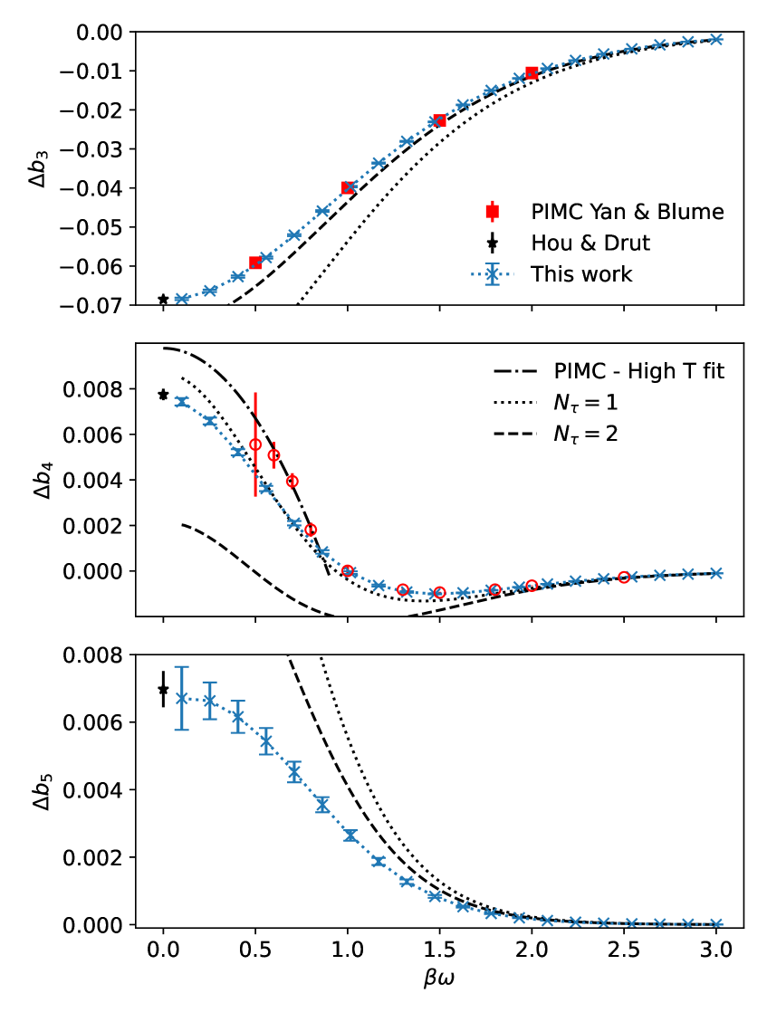
Figure 1: $\Delta b_{3}$ (top), $\Delta b_{4}$ (middle), and $\Delta b_{5}$ (bottom) as functions of $\beta\omega$, for a trapped unitary Fermi gas. Our results are shown with blue crosses and error bars, joined by a blue dotted line. The data by Yan and Blume from Ref. [28] appears as red squares for $\Delta b_{3}$ and red circles for $\Delta b_{4}$, in both cases with error bars. The dashed-dotted line in the middle plot shows a high-temperature fit to the data of Ref. [28]. Black stars with error bars show the results by Hou and Drut from Ref. [40] calculated in the homogeneous gas limit. The dotted (dashed) line shows the $N_{\tau}=1$ ($N_{\tau}=2$) results given analytically in the Supplemental Materials. The latter show that, for $\Delta b_{3}$, increasing $N_{\tau}$ from 1 to 2 shows a dramatic improvement, whereas the case of $\Delta b_{4}$ is a cautionary tale: as $N_{\tau}$ goes from 1 to 2, the results move away from our final answer (blue crosses). In fact, it is not until $N_{\tau}=5$ that $\Delta b_{4}$ reaches the asymptotic regime one can use for extrapolation. Reference [29] presented a large-$\beta\omega$ asymptotic formula for $\Delta b_{n}$, but its validity is well outside the $0<\beta\omega<3$ region studied here.

Results: Virial coefficients in the unitary limit.- In our approach, we calculate $\Delta b_{2}$ as a function of the bare coupling $C$, $\beta\omega$, and $N_{\tau}$, and renormalize by tuning $C$ to the known result in the unitary limit [12], namely $\Delta b_{2}=\left[4\cosh(\beta\omega/2)\right]^{-1}.$ Thus, the second-order VE is reproduced exactly by virtue of this renormalization condition, such that the line of constant physics is followed in the extrapolation to $N_{\tau}\to\infty$, for each $\beta\omega$ (see Supplemental Materials of Ref. [40]).

In Fig. 1 we show our results for $\Delta b_{3}$ (top), $\Delta b_{4}$ (center), and $\Delta b_{5}$ (bottom) for a unitary Fermi gas in a harmonic trap as a function of $\beta\omega$. The error bars represent the uncertainty in the $N_{\tau}\to\infty$ extrapolation, given by the difference between the maximum and minimum predictions of polynomial extrapolation schemes (degrees 2 to 5 for $\Delta b_{3}$ and $\Delta b_{4}$, and degrees 2 and 3 for $\Delta b_{5}$, where the data is more limited; see Ref. [40]). Our results for $\Delta b_{3}$ are in superb agreement with the quantum Monte Carlo data of Ref. [28] as well as with the homogeneous-limit answer of Ref. [40]. [The homogeneous limit is related to the results shown here by $\Delta b_{n}^{\mathrm{h}}=n^{3/2}\Delta b_{n}(\beta\omega\to 0)$, see Refs. [46, 12, 22, 23]]. The case of $\Delta b_{4}$ is less clear cut: there is good agreement with Ref. [28] for $\beta\omega\geq 1$, but a clear difference remains at low frequencies. We return to this issue below. Finally, we predict $\Delta b_{5}$ as a function of $\beta\omega$, which to the best of our knowledge does not appear elsewhere in the literature. As the HO potential confines the system, it naturally increases its kinetic energy, effectively reducing the interaction effects. This suggests that, for a given interaction strength, the VE should enjoy better convergence properties when a trapping potential is turned on (as argued also in Ref. [12]). Indeed, although our results indicate that $\Delta b_{4}\simeq\Delta b_{5}$ and, moreover, for $0.3<\beta\omega<1.4$ we find $\Delta b_{5}>|\Delta b_{4}|$, we also find that $|\Delta b_{2}|\gg|\Delta b_{3}|\gg|\Delta b_{4}|$.

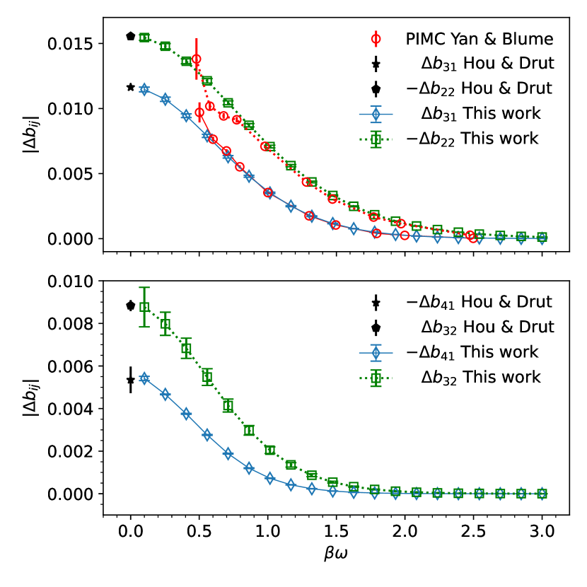
Figure 2: Top: $\Delta b_{31}$ (blue diamonds) and $-\Delta b_{22}$ (green squares) as functions of $\beta\omega$, compared with the PIMC results of Ref. [28] (red circles joined by solid line for $\Delta b_{31}$ and joined by a dotted line for $\Delta b_{22}$). The black star and black pentagon show, respectively, the results for $\Delta b_{31}$ and $-\Delta b_{22}$ in the $\beta\omega\to 0$ limit, obtained in Ref. [40]. Bottom: $-\Delta b_{41}$ (blue diamonds) and $\Delta b_{32}$ (green squares) as functions of $\beta\omega$. The black star and black pentagon show, respectively, the results for $-\Delta b_{41}$ and $\Delta b_{32}$ at $\beta\omega=0$ from Ref. [40].

To better understand the differences in $\Delta b_{4}$ between our results and Ref. [28], we plot in Fig. 2 (top panel) the subspace contributions $\Delta b_{31}$ and $\Delta b_{22}$. As pointed out in Ref. [28], these contributions partially cancel each other out, leading to the observed increased uncertainty in the final answer. Clearly, the largest differences arise in the determination of $\Delta b_{22}$, which is not unexpected as a contact interaction in that subspace is less susceptible to Pauli blocking than $\Delta b_{31}$.

Figure 2 (bottom panel) shows our results for $\Delta b_{41}$ and $\Delta b_{32}$, whose behavior parallels $\Delta b_{31}$ and $\Delta b_{22}$ in that they enter with different signs but similar magnitude, thus leading to increased uncertainty in the final result for $\Delta b_{5}$. In spite of those delicate cancellations, we are able to resolve the fifth-order contribution, as shown already in the bottom panel of Fig. 1. Nevertheless, the size of the error bars of $\Delta b_{32}$ is larger than that of $\Delta b_{41}$. This may come as a surprise given the results of Ref. [40], whose uncertainty at $\beta\omega=0$ for $\Delta b_{41}$ is larger than for $\Delta b_{32}$. Those results were calculated at the same $N_{\tau}=9$ order for both coefficients, using an analytic cancellation of volume-dependent terms. In contrast, in the present work we achieved $N_{\tau}=12$ for $\Delta b_{41}$ but only $N_{\tau}=8$ for $\Delta b_{32}$, due to the increasing computational cost of cancelling the volume-dependent terms, which is done numerically in the trapped case.

Results: Applications to thermodynamics.- Having obtained the precise form of $\Delta b_{3}$, $\Delta b_{4}$, and $\Delta b_{5}$ as functions of $\beta\omega$ for harmonically trapped fermions in the unitary limit, we apply those results to obtain thermodynamic information. As an example, we report here the compressibility and magnetic susceptibility, respectively $\chi_{n}$ and $\chi_{s}$, defined as $\chi_{n,s}=\beta^{-1}\partial^{2}\ln\mathcal{Z}/\partial h_{\pm}^{2}$, where $h_{\pm}=(\mu_{\uparrow}\pm\mu_{\downarrow})/2$ and $\mu_{s}$ is the chemical potential for spin-$s$ particles. The interaction effects on $\chi_{s,n}$ are

$$\Delta\chi_{n,s}=\frac{\lambda_{T}^{2}}{8\pi}Q_{1}\sum_{n=3}^{\infty}\sum_{m+j=n}(m\pm j)^{2}\Delta b_{mj}z_{\uparrow}^{m}z_{\downarrow}^{j},$$ (15)

where $z_{s}=e^{\beta\mu_{s}}$ is the fugacity for spin-$s$ particles.

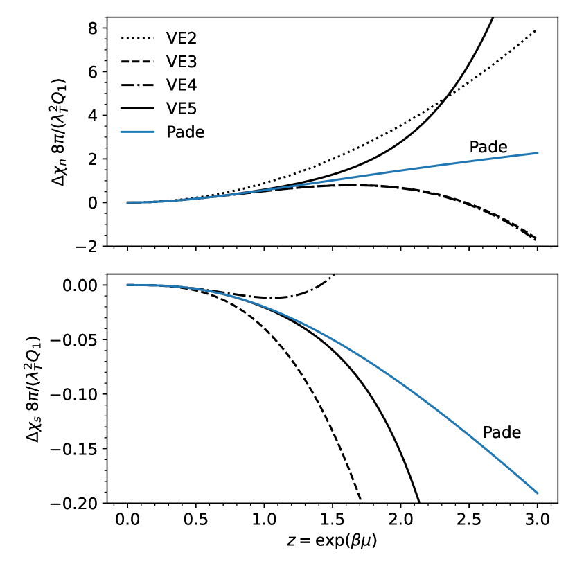
Figure 3: Top: Interaction effects on the compressibility $\Delta\chi_{n}$, in units of $8\pi/(\lambda_{T}^{2}Q_{1})$, as a function of the fugacity $z$ for a harmonically trapped unitary Fermi gas at $\beta\omega=1$. The second, third, fourth, and fifth-order VE results are shown, respectively, with dotted, dashed, dash-dotted, and solid lines. The Padé resummed result (with a $[3/2]$ approximant) is shown as a blue line. Bottom: Interaction effect on the magnetic susceptibility $\Delta\chi_{s}$ as a function of $z$, for the same parameters as in the top panel. The second-order VE is omitted because it is identically zero for $\Delta\chi_{s}$.

Our results, shown in Fig. 3, indicate that the partial sums of the VE display large variations for $\Delta\chi_{n,s}$ as the VE order is increased, in particular for $z\geq 1$. However, we also see that, using the high-order coefficients we calculated here, it is possible to carry out a Padé resummation [and related strategies (see e.g. [47])] to obtain sensible results for static response functions even as far as $z=3$.

Conclusion and outlook.- In this work we have determined the frequency dependence of the virial coefficients $b_{n}$ of HO-trapped spin-$1/2$ fermions at unitarity. We used a discretization of the imaginary time direction and a Suzuki-Trotter factorization of the transfer matrix, together with automated algebra methods, to calculate canonical partition functions and from them the interaction induced change $\Delta b_{n}$, for $n=3,4,5$, which we extrapolated to the continuous-time limit. To complement those numerical results, we provided analytic formulas for $\Delta b_{n}$ in coarse lattices for arbitrary trap frequency and spatial dimension. Using our final $\Delta b_{n}$, we calculate the compressibility and susceptibility of the unitary Fermi gas and showed that the VE can be Padé-resummed to obtain sensible results even as far as $z=3$.