Quantum f(R) gravity and AdS/CFT

Abstract

We propose to study the entanglement entropy in braneworld modified gravity. We show that the $d+1$-dimensional action $I_{d+1}$ is the dual of $d-1$-dimensional entanglement entropy $S_{d-1}^{EE}$. Moreover, we remark that the generalization of action-entropy shows us a new form of $f(R)$ gravity which is in good agreement with the most choices of $f(R)$ gravity in the literature. We show also that there are two copies of the AdS spaces in holographic entanglement $f(R)$ gravity. We have proposed that the time is a holographic projection of the hidden $d$-brane on the visible $d$-brane. To determine the geometry of this holographic projection, we have used the $AdS_{2}$ geometry of the black hole. Namely, the past of events is memorized over an $\mathbb{S}^{1}$. We show that the time projection is a stereographic projection from a time sphere $\mathbb{S}^{d-2}$ on the hidden $d$-brane to the visible $d$-brane. We suggest that there is a difference between the time in classical gravity and the time in quantum gravity.

1 Introduction

Modified gravity is an alternative approach that generalizes Einstein’s theory of general relativity. One of the most successful alternative gravity theories is $f(R)$ gravity [1]. The previous studies on $f(R)$ gravity have been executed in the standard metric formalism in $4d$. The $f(R)$ formalisms derive the gravitational field equation from the action. There exist other of types of $f(R)$ gravity, for example $f(R)$ braneworld models [2]. Also we have holographic $f(R)$ gravity [3]. In this paper we are interested in studying the braneworld and the black holes by the $f(R)$ gravity. The $f(R)$ gravity is the simplest generalization of general relativity. Various studies have assessed the efficacy of $f(R)$ gravity. Hawking had succeeded in demonstrating his famous black hole area theorem [4]. Information paradox opposing the laws of quantum mechanics to those of general relativity. Indeed, general relativity implies that information could fundamentally disappear in a black hole, following the evaporation of this one. This loss of information implies a non-reversibility (the same state can come from several different states), and a non-unitary evolution of quantum states, in fundamental contradiction with the postulates of quantum mechanics [5]. In 2019, Penington and al. discovered a class of semi-classical space-time geometries that had been overlooked by Hawking and later researchers [6, 7]. Penington et al. calculate entropy using the cue trick and show that for sufficiently old black holes, we must consider solutions in which the aftershocks are connected by wormholes. The inclusion of these wormhole geometries prevents entropy from increasing indefinitely [7, 8]. To date, several studies have investigated the holographic theory [9, 10]. This was essentially found by remembering that the entropy of a black hole: the Bekenstein-Hawking formula $S_{BH}=\frac{Area\left(\Sigma\right)}{4G_{N}}$ [11]. We recall the holographic entanglement entropy formula introduced by Ryu and Takayanagi [12]: $S_{BH}=\min\frac{Area\left(\gamma\right)}{4G_{N}^{d+1}}$, where $\Sigma$ is the horizon, $\gamma$ is the bulk surface and $G_{N}$ is the Newton constant. Ryu and Takayanagi proposed that the entanglement entropy associated with a spatial region in a holographic QFT is given by the particular minimal area surface in the dual geometry. AAccording to this description, the degrees of freedom contained in a certain region of gravity are proportional to its area of the event horizon $\Sigma$ instead of the volume. This correspondence between a geometric quantity and a microscopic data is the key concept of holography. The AdS/CFT correspondence [13] proposed by J. Maldacena; is a conjecture connecting two types of theories: Conformal field theories (CFT) occupy one side of the correspondence; they are quantum field theories which include theories similar to those of Yang-Mills which describe elementary particles. On the other hand, anti Sitter spaces (AdS) are theories of quantum gravity, formulated in terms of string theory (or M theory). More recently, the notion of the extended holographic entanglement entropy proposes to relate the holographic QFT with the $f(R)$ models [14, 15].
In this paper, we propose to study $d$-dimensional $f(R)$ gravity within the framework of holographic entanglement theory. Our aim in this paper is to determine the nature of the time. To study the time, it is necessary to study first the entropy. In particular, the holographic entanglement entropy.
This paper is organized as follows: In section 2, we will examine the $f(R)$ gravity in the bulk with two branes. In section 3, we study the results of the previous section, in comparison with the Randall-Sundrum (RS) model. In section 4, we use the results of sections 2 and 3 to describe stereographic projection of time in the black hole; by the $AdS_{2}$ geometry then by two $CFT$, finally in the context of $AdS_{d+1=5}/CFT_{d=4}$. In section 5, we introduce a general description of the stereographic projection of time. Section 6 focuses on the study of the previous results, particularly, the difference between the time on the classical scale and on the quantum scale. We conclude in the final section.

2 Topological aspects of f(R) gravity

2.1 Generalization of action and entropy

We start with the full bulk manifold $M_{d+1}$, and we define the full boundary $B_{d}$ $=\partial M_{d+1}$ by the flat Minkowski spacetime $R^{1,d-1}$. In particular, we can choose $M_{d+1}=AdS_{d+1}$ and $B_{d}=CFT_{d}$. The bulk $M_{d+1}$ described by the field theory and $B_{d}$ is conformal boundary. The QFT resides on a background geometry $B_{d}$ foliated by Cauchy surfaces $\Sigma_{t(d-1)}$. The $\Sigma_{t(d-1)}$ is fixed-time slice with $\Sigma_{t(d-1)}=A_{d-1}\cup B_{d}$, where $A_{d-1}\$is a subregion of $\Sigma_{t}$. $\partial A_{d-2}$ is the entangling surface. $\varepsilon_{d-1}$ is RT minimal surface with boundary entaglement $\partial\varepsilon_{d-2}=\partial A_{d-2}=\varepsilon_{d-1}\cap B_{d}$, which gives the entropy formula $S_{A}=\frac{1}{4G_{N}^{(d+1)}}Area(\varepsilon_{d-1})$. [18]. The general action of $f(R)$ gravity is written as

$$I_{4}=\frac{M_{p}^{2}}{2}\int_{M_{4}}d^{4}x\sqrt{g_{4}}f(R)+I_{m},$$ (2.1)

where $M_{p}^{2}=\frac{1}{8\pi G}$ is the Planck mass, $I_{m}$ is the matter action and $R$ is the Ricci scalar on the spacetime $R^{1,3}\supset\left(M_{4},g_{\mu\nu 4}\right)$ defined by a metric $g_{\mu\nu 4}$, such as $g_{4}=\det g_{\mu\nu 4}$ and $(\mu,\nu=0,1,2,3)$. We use system of units the constants (speed of light $c$, reduced Planck constant $\hbar$, Boltzmann constant $k_{B}$ and Newton’s constant $G$) are equal to $1$: $c=\hbar=k_{B}=G=1$. Now let us consider the Planck mass in $d+1$-dimensional $M_{d+1}^{d-1}=M_{p}^{2}/L^{d-3}$, such as $L$ is the radius of the large compact dimension. Moreover, we consider a conformal transformation which transforms the $d=4$ metric $g_{\mu\nu\left(4\right)}$ (of $M_{4}$) to $d+1$-dimensional metric $g_{MN\left(d+1\right)}$, (of $M_{d+1}$) where $(M,N=0,1,...,d)$. Thus, the $d+1$-dimensional action is written as

$$I_{d+1}=\frac{1}{2}M_{d+1}^{d-1}\int_{M_{d+1}}d^{d+1}x\sqrt{g_{\left(d+1\right)}}f(R).$$ (2.2)

Let us now introduce the EE formula in $f(R)$ gravity which is already used in the literature [15, 19], generalized with $d-1$-dimensional metric $g_{\mu\nu\left(d-1\right)}$, which is written as

$$S_{d-1}^{EE}=-2\pi M_{d+1}^{d-1}\int_{A_{d-1}}d^{d-1}x\sqrt{g_{\left(d-1\right)}}F(R),$$ (2.3)

with $F(R)=\frac{\partial f(R)}{\partial R}=\partial_{R}f(R)\in A_{d-1}$ and $\ f(R)\in M_{d+1}$, the region $A$ is fixed on time slice $\Sigma_{t(d-1)}=A_{d-1}\cup B_{d}$ with $\ B_{d}$ $=\partial M_{d+1}$. Thus, $M_{d+1}$ and $A_{d-1}\subset B_{d}$ connected by homomorphisms called boundary operators or differentials $\partial_{R}$ according to the Ricci scalar $R$. The expressions of $I_{d+1}$ and $S_{d-1}^{EE}$ belongs in $M_{d+1}$ and $A_{d-1}$ respectively, i.e. $I_{d+1}\sim Vol_{d+1}f(R)$ and $S_{d-1}^{EE}\sim Vol_{d-1}\partial_{R}f(R)$, such as $Vol_{d}=\int\omega_{d}=$ $\int d^{d}x\sqrt{g}$. We suppose that $I_{d+1}$ gives us the information on the gravity in $M_{d+1}$ and $S_{d-1}^{EE}$ is the projection of gravity information from $M_{d+1}$ to $A_{d-1}$. We will prove this proposition in the next sections.

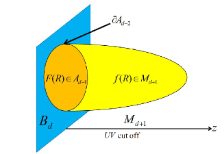
Figure 1: $F(R)$ gravity focuse on studying the region $A_{d-1}$. $A_{d-1}$ associated with the entanglement surface $\partial A_{d-2}$ . $f(R)$ gravity describes $M_{d+1}$.

the two Eqs.(2.2,2.3) becomes

$$I_{d+1}=\frac{1}{2}\left(-4\pi\right)^{0}M_{d+1}^{d-1}Vol_{d+1}f(R),$$ (2.4)

$$S_{d-1}^{A}\equiv S_{d-1}^{EE}=\frac{1}{2}\left(-4\pi\right)^{1}M_{d+1}^{d-1}Vol_{d-1}\partial_{R}f(R).$$ (2.5)

The $d+1$-dimensional Planck mass $M_{d+1}^{d-1}$ is a tool that connects $M_{d+1}$ and $A_{d-1}$, i.e. $M_{d+1}^{d-1}:d-1\longrightarrow d+1$. We notice the gravity at $\left(d+1\right)$ is described by the action, on the other hand the gravity on $\left(d-1\right)$ described by the entropy. The action $I_{d+1}$ and entropy $S_{d-1}^{A}$, they have a physical significances, let’s generalize now the two expressions (2.4) and (2.5) by a single term:

$$U\left(d+\left(-1\right)^{\delta}\right)=Vol_{d+\left(-1\right)^{\delta}}\left(-4\pi\partial_{R}\right)^{\delta}\left(\frac{1}{2}M_{d+1}^{d-1}f(R)\right)\text{,}$$ (2.6)

where $\delta=\left\{0,1\right\}$. To shorten this relationship, we write $U\left(d-1\right)=S_{d-1}^{A}$ and $U\left(d+1\right)=I_{d+1}$. But if we choose arbitrarily $\delta\longrightarrow-\infty$, one can obtain $U\left(d\right)=cte$. The expression of $U$ is equivalent to two states corresponding to the couple $\left(I_{d+1},S_{d-1}^{A}\right)$. The other values of $U$ don’t have a physical interpretation.

2.2 f(R) solutions

The term $d+\left(-1\right)^{\delta}$ in Eq.(2.6) equal to $d-1$ for these two values $\delta=\left\{-1,1\right\}$, i.e. for the value $\delta=-1$, we obtain $U\left(d-1\right)=S_{d-1}^{A}$ which has a physical interpretation. We then want to study the case where $\delta=-1$ and we compare the result of this value with that of $\delta=1$. If we take the symmetry $U\left(d-1,\delta=1\right)=U\left(d-1,\delta=-1\right)$, and the condition $\partial_{R}\partial_{R}^{-1}=1$, we find this differential equation $\partial_{R}^{2}f(R)-\frac{M^{2}}{\left(4\pi\right)^{2}}f(R)=0$, its solution is of the form

$$f(R)=f^{+}e^{\frac{RM^{2}}{4\pi}}+f^{-}e^{-\frac{RM^{2}}{4\pi}},$$ (2.7)

where $\left(f^{-},f^{+}\right)$ are integration constants, and $M$ is a mass parameter. It is evident that for small $R$ the running $f(R)$ depends more dramatically on $\left(f^{-},f^{+}\right)$, i.e. the gravity in a Ricci flat solution is not zero: $f(R_{0})=R_{0}=f^{+}+f^{-}$. This solution shows us that $f^{+}+f^{-}$ represents the $f(R)$ gravity in the vacuum. For $AdS_{d+1}$ spacetime $\left(R\preceq 0\right),$ when $R\longrightarrow-\infty$, the running diverges as $f(R)\sim$ $f^{-}e^{-\frac{RM^{2}}{4\pi}}$. When $R\longrightarrow+\infty$: $f(R)\sim f^{+}e^{\frac{RM^{2}}{4\pi}}$. We examine the nature of the couple $\left(f^{+},f^{-}\right)$ in the next section, and we will answer this question: why we have two gravity fields?. Let us now discuss the various forms of $f(R)$ (2.7): This value is very close to choosing of $\ f(R)$ for the transition between 4d and 5d [20]. If we choose $R\sim 0$ we find $f(R)=\frac{M^{2}}{4\pi}\left(f^{+}-f^{-}\right)R+\left(f^{+}+f^{-}\right)$; this expression is equivalent to the standard expression $f(R)=P\left(\phi\right)R+Q\left(R\right)$ as considered in [21, 22], since $\left(f^{-},f^{+}\right)$ doesn’t depend on $R$ . If $\left(f^{+}-f^{-}\right)=\frac{4\pi}{M^{2}}$ and $\left(f^{+}+f^{-}\right)=\Lambda$,  one can obtain $\Lambda$CDM cosmology [23]. On the other hand, if we expand (2.7) in second order, and if we take $f^{+}=-f^{-}$, we find a form close to Starobinsky model [24]: $f(R)=\frac{f^{+}M^{2}}{2\pi}R+\frac{f^{+}M^{4}}{\left(4\pi\right)^{2}}R^{2}$. We can remark that $f(R)$ (2.7) is expressed in Kruskal coordinates [25]: $\left(U\equiv-e^{-\frac{RM^{2}}{4\pi}},V=e^{\frac{RM^{2}}{4\pi}}\right)$ with $V=-U^{-1}$. This last condition is equivalent with

$$T^{2}-X^{2}=-1\prec 1\text{.}$$ (2.8)

The transformation brings the coordinates in the form $T=\frac{1}{2}\left(U+V\right)$,   $X=\frac{1}{2}\left(V-U\right)$. Therefore, we can express the geometric characteristics of $f(R)$ in conformal diagrams (Penrose diagrams).  We choose the coordinates in this way $U=-e^{-\frac{RM^{2}}{4\pi}},V=e^{\frac{RM^{2}}{4\pi}}$ and we assume that $M$ is Schwarzschild mass parameter [26].   

$$f(R)=f^{+}V-f^{-}U.$$ (2.9)

The above equation is written with Kruskal-Szekeres coordinates on the bulk manifold $M_{d+1}$ are defined, from the Schwarzschild coordinates, by replacing $\left(t,x_{1},,...,x_{d}\right)$ by a new timelike coordinate $T$ and a new spacelike coordinate $X\in M^{c}$, with $M^{c}$ is the conformal manifold of $M_{d+1}$ in $2d$. The coordinates of Kruskal-Szekeres, have the advantage of covering the whole space-time of the Schwarzschild solution extended to the maximum and behave well everywhere apart from the physical singularity. Eq.(2.9) implies that

$$f(R)=\left(f^{+}-f^{-}\right)T+\left(f^{+}+f^{-}\right)X.$$ (2.10)

We have already shown in Ricci flat solution (in the vacuum of $M_{d+1}$) that: $R_{0}=f^{+}+f^{-}$. We want to write $f(R)$ in the vacuum. From (2.10) it is evident that

$$f(R)\sim\frac{\chi\left(T,X\right)}{R_{0}}+R_{0},$$ (2.11)

where $\chi\left(T,X\right)$ is a function of $T$ and $X$. This last equation is equivalent to the form of $f(R)$ proposed in [27]. According to [28], the term $1/R_{0}$ represents the evolution of dark energy. The Ricci flat solution $R_{0}$ describes gravity in the vacuum, i.e. $R_{0}$ describes the gravity of the matter.

2.3 Field equations solution: two density

In this subsection, we will consider the function (2.7), to calculate the action (2.2) and the entropy (2.3). Then we use two conformal transformations in metric determinant

$$g_{\sigma}\longrightarrow g_{\sigma}^{\pm}=g_{\sigma}e^{\pm\frac{RM^{2}}{2\pi}}\text{,}$$ (2.12)

where $\sigma=\left\{\left(d-1\right)\text{ or }\left(d+1\right)\right\}$. The two conformal transformations leads to

$$I_{d+1}=\frac{1}{2}M_{d+1}^{d-1}\int_{M_{d+1}}d^{d+1}x\left(\sqrt{g_{d+1}^{-}}f^{-}+\sqrt{g_{d+1}^{+}}f^{+}\right),$$ (2.13)

$$S_{d-1}^{A}=\frac{1}{2}M_{d+1}^{d-1}\int_{A_{d-1}}d^{d-1}x\left(\sqrt{g_{d-1}^{-}}f^{-}-\sqrt{g_{d-1}^{+}}f^{+}\right).$$ (2.14)

These two formulas show that there are two essential terms in the holographic entanglement $f(R)$ gravity: the two fields $\left(f^{-},f^{+}\right)$, describes the gravity in $M_{d+1}$ and $A_{d-1}$. These two fields replace the Ricci scalar in the Einstein Hilbert action for high gravity. The classical gravity fields in Eqs.(2.13,2.14) are similar to quantum operator field in quantum gravity, this vision will help us later to describe gravity in the quantum and classical framework. Eqs.(2.13,2.14) consists of two essential parts: $I_{d+1}=I^{-}+I^{+}$ and $S_{d-1}^{A}=S^{-}-S^{+}$; the first equation describes the induced gravity on $M_{d+1}$ by double copies of action, which corresponds to the gravity dual [29]. The last equality is a special case of the classical Araki-Lieb inequality [30]. Let us now calculate the field equations from (2.13):

$$\delta I_{d+1}\sim\sum_{\sigma=-,+}\delta g^{\sigma MN}\sqrt{g_{d+1}^{\sigma}}\left(\frac{\delta f^{\sigma}}{\delta g^{\sigma MN}}-\frac{1}{2}g_{MN\left(d+1\right)}^{\sigma}f^{\sigma}\right).$$ (2.15)

We assume that the action $I_{d+1}$ is the sum of two sub-actions $I_{d+1}=I^{-}+I^{+}$, i.e. $\delta I^{-}=\delta I^{+}=0$. Since $f^{\pm}$ does not depend on $R$ (2.7), then the term $\frac{\delta f^{\pm}}{\delta g^{\pm MN}}$ must be zero. Thus, the field equations are given by

$$T_{MN}^{\pm}=-\frac{1}{2}M_{d+1}^{d-1}g_{MN\left(d+1\right)}^{\pm}f^{\pm},$$ (2.16)

which leads to

$$\rho^{\pm}=g^{\pm MN}T_{MN}^{\pm}=-\frac{d+1}{2}M_{d+1}^{d-1}f^{\pm},$$ (2.17)

where $\rho^{\pm}$ represents the matter mass-energy density. Starting with the static solution above, we remark that the above consequence shows that the distribution of matter is tied to the fields $\left(f^{-},f^{+}\right)$ and the number of space-time dimensions. Moreover, we have two distributions of matter $\left(\rho^{-},\rho^{+}\right)$. Since Eq.(2.7) is a solution of gravity on the bulk manifold $M_{d+1}$, which implies that the fields $f^{\pm}$ exist in the bulk. On the other hand, we can write $\rho^{\pm}=\rho_{dbrane}^{\pm}+\rho_{bulk}^{\pm}$. This relation shows us that the matter present in $d$-brane $\left(\rho_{dbrane}^{\pm}\right)$, but there is also another density outside of the $d$-brane, i.e. there is a strange matter in the bulk $\left(\rho_{bulk}^{\pm}\right)$, it can be the dark matter. Using Eq.(2.17) one can obtain

$$\left(d+1\right)L=\text{\ }\left(\rho^{-}-\rho^{+}\right)T-\left(\rho^{-}+\rho^{+}\right)X.$$ (2.18)

This shows that there is a remarkable symmetry; the Lagrangian $L$ is invariant under the following symmetry:

$$\rho^{-}\longleftrightarrow T\text{ };\text{ }\rho^{+}\longleftrightarrow X.$$ (2.19)

Using Eq.(2.18), we see that the dependent Lagrangian consists of a spatial Lagrangian $L_{X}\sim$ $-\left(\rho^{-}+\rho^{+}\right)X$ and a temporal Lagrangian $L_{T}\sim$ $\left(\rho^{-}-\rho^{+}\right)T$. In the next section, we will determine the nature of the densities $\left(\rho^{-},\rho^{+}\right)$.

3 Two d-brane

Our goal in this section, is to determine the quantum aspect of the action (2.13) and the entropy (2.14), since they look like writing quantum fields. From Eqs.(2.13) and (2.14), we remark that the above consequence can be shown that $I_{d+1}$ is invariant under the transformations $\left(g_{{}^{-}},f^{-}\right)_{d+1}\longrightarrow\left(g_{{}^{+}},\left(-1\right)^{\delta}f^{+}\right)_{d+1}$ for $\delta=0$ . And $S_{d-1}^{A}$ is invariant under the transformations: $\left(g_{{}^{-}},f^{-}\right)_{d-1}\longrightarrow\left(g_{{}^{+}},\left(-1\right)^{\delta}f^{+}\right)_{d-1}$ for $\delta=1$. Using the complex writing one can obtain

$$f_{d\pm 1}^{-}\longrightarrow e^{i\pi\delta}f_{d\pm 1}^{+},$$ (3.1)

which implies an invariance of the action-entropy under a global internal $U(1)$ transformation (gauge group). The field $f^{+}$ is just a rotation of the phase angle of the field $f^{-}$, with a particular rotation determined by the constant $\pi\delta$. Which is the result of the self-duality property of the $U(1)$ gauge theory [31]. i.e. the field $f^{+}$ is the dual of field $f^{-}$ in the context of gravity dual. Let $\phi=\pi\delta$, according to Eq.(2.6) we only have two values of $\phi$: are $\phi=0$ and $\phi=\pi$. These values correspond exactly with the location of two 3-branes in the Randall-Sundrum model (RS model) [32]. This shows that there is two $d$-brane $B_{d}$ in the full bulk $M_{d+1}$. Which explains why we have double gravity fields $\left(f^{-},f^{+}\right)$ in a vacuum. The fields $f^{-}$ and $f^{+}$ exist mainly in $d$-branes located at $\phi=0$ and $\phi=\pi$ respectively. We can have the fields $\left(f^{-},f^{+}\right)$ in the bulk where $0\preceq\phi\preceq\pi$. Thus, $\phi$ is the coordinate for extra dimensions. We notice the orbifold symmetry: $\phi\longrightarrow-\phi$, i.e. the orbifold fixed points at $\phi=0$, $\phi=\pi$. According to the RS model, we can express the metrics of the $d$-branes $g_{d-1}^{-}$, $g_{d-1}^{+}$ according to the bulk metrics $g_{d+1}^{-}$, $g_{d+1}^{+}$ as

$$g_{\mu\nu\left(d-1\right)}^{-,hid}\left(x^{\mu}\right)=g_{\mu\nu\left(d+1\right)}^{-}\left(x^{\mu},\phi=0\right)\text{,}$$ (3.2)

$$g_{\mu\nu\left(d-1\right)}^{+,vis}\left(x^{\mu}\right)=g_{\mu\nu\left(d+1\right)}^{+}\left(x^{\mu},\phi=\pi\right).$$ (3.3)

Since we have two metrics in the bulk, then the bulk is the union of two copies of submanifold $M_{d+1}=M_{d+1}^{-}\cup M_{d+1}^{+}$ [15]. This last equation can help us identify the densities (2.17): $\rho^{-}=\rho_{hid}+\rho_{bulk}$, where $\rho^{hid}$ represents the density of matter in the hidden $d$-brane or dark matter (DM) density and $\rho^{+}=\rho_{vis}+\rho_{bulk}$, where $\rho^{vis}$ represents the density of matter in our $d$-brane and $\rho_{bulk}$ is the bulk density (or dark energy density). Generally, we write

$$\rho_{vis}=\rho_{matter}\text{ \ \ }\rho_{hid}=\rho_{DM}\text{\ }\ \ \text{\ }\rho_{bulk}=\rho_{DE}.$$ (3.4)

From the symmetry (2.19); the density in the visible $d$-brane related with the volume of the spatial part $X$: $\rho_{vis}\sim T$. On the other hand, the density in the hidden $d$-brane connected with the temporal part $T$: $\rho_{hid}\sim X$. We can see that the time is a property of the hidden $d$-brane. It is difficult to imagine that time is a dimension that does not belong to the visible $d$-brane. Maybe the notion of time doesn’t exist in our d-brane is the answer to this question: if time is a dimension in the visible d-brane, why we can’t move freely in time like spatial dimensions?. We propose in this case that time is an external property of the visible $d$-brane. Most physical graders are derivatives over time, which means, that the physical quantities are connections between the visible spatial (visible $d$-brane) part and the hidden temporal part (hidden $d$-brane). The measurement in visible $d$-brane is done concerning the referential of hidden $d$-brane. Also, the measures in hidden $d$-brane are done concerning the space of the visible $d$-brane. In this scenario Eq.(2.8) become $X^{2}+\left(iT\right)^{2}=1$. The complex term $iT$ shows that time is a hidden dimension. Because if we take a physical phenomenon described by a complex number $z=x+iy$, the real part $x$ represents the visible face of $z$, and the hidden face is described by the imaginary part $y$. We can see this logic, in physics, like that: The general relativity describes the cosmic phenomena (visible) within a framework of real numbers. And that quantum mechanics describes the microscopic scale (hidden) by complex numbers, with the same principle, time exists in the hidden $d$-brane, and that the presence of the time in our Universe is a holographic projection of real-time in hidden $d$-brane on visible $d$-brane.
Let us now $I_{d+1}=I^{-}+I^{+}$; we have $I^{-}=I_{d}^{hid}+I_{d+1}^{bulk}$ , $I^{+}=I_{d}^{vis}+I_{d+1}^{bulk}$. Hence, $I_{d+1}=I_{d}^{hid}+\ I_{d}^{vis}\ +\ 2I_{d+1}^{bulk}$, this also agrees with the induced gravity action found by [15]; this paper treats $f(R)$ gravity in the bulk in the context of the RS model.

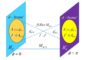
Figure 2: Two brane located in the bulk. Our brane located on the position $\phi=\pi$ and the hidden brane located on $\phi=0$.

The orbifold symmetry of $\phi$ implies that $g_{\mu\nu\left(d+1\right)}^{-}\left(x^{\mu},\phi=0\right)=g_{\mu\nu\left(d+1\right)}^{+}\left(x^{\mu},\phi=\pi\right)$ in $\phi=\pi/2$; i.e. $M_{d+1}$ have periodic boundary conditions in $\phi=\pi/2$. Moreover, string theory describes the graviton by the metric, which implies that the last condition describes the closed string [33]. Therefore, our model perfectly describes the gravitons $g_{\mu\nu}$ (closed strings) in the region $\phi=\pi/2$.  In $M_{d+1}\left(\phi=\pi/2\right)$, the two bulk geometry must be the same; we will have $g_{d+1}^{-}=g_{d+1}^{+}$ ; $f^{-}=f^{+}$, which implies that $S_{d-1}^{A}\left(\phi=\pi/2\right)\sim M_{d+1}^{d-1}$ and $I_{d+1}\left(\phi=\pi/2\right)\sim S_{d-1}^{A}Vol_{d+1}f^{+}$. From [32]; the extra-dimensional coordinate $z$ is expressed in terms of the compactification radius $r_{c}$ and the angular coordinate $\phi$ by $z=r_{c}\phi$. Lorentz’s formulas make it possible to express the coordinates $(t_{+},\mathbf{x}_{+}^{d-1},z)$ of a given event in the hidden $d$-brane ” assumed fixed” frame of reference as a function of the coordinates $(t_{-},\mathbf{x}_{-}^{d-1},z)$ of the event in the ”mobile” visible $d$-brane. One of Lorentz’s formulas can be written as

$$t_{-}-t_{+}\sim z.$$ (3.5)

This result shows that time is the displacement of visible $d$-brane concerning the hidden $d$-brane, each point in $B_{d}^{+}$ depends on another point on $B_{d}^{-}$. Additionally, the presence of two gravitational fields $\left(f^{-},f^{+}\right)$ in the Lagrangian (2.7), is very similar to the Lagrangian expression in dual gravity [34, 35]. According to our model; $f^{+}\in$ the visible $d$-brane and $f^{-}\in$ the hidden $d$-brane. If we assume that $f^{+}$ is a graviton then $f^{-}$ is a dual graviton [36]. The dual of the graviton predicted by some formulations of $SO(8)$ supergravity in the framework of electric-magnetic duality emerged in the $E_{11}$ in eleven dimensions, as an S-duality. According to the dual gravity theory [37], it is no local coupling between graviton and dual graviton. Which corresponds exactly with the Lagrangian expression (2.7); we see that there is no coupling between $f^{+}$ and $f^{-}$.We apply the symmetry (2.19) on Eq.(2.17), it is useful to rewrite the transformation of symmetry: $\left(\ f^{-},\ f^{+}\right)\sim\left(T,X\right)$. This result shows us that the double gravity fields occupy $d$-brane space-time by a space field $f^{+}$ and another time field $\ f^{-}$. We propose that a properties (ex: time) of the visible $d$-brane with the coordinates $(t_{+},\mathbf{x}_{+}^{d-1},z)$ are holographic entanglement of a proporities the hidden $d$-brane with the coordinates $(x_{-},\mathbf{t}_{-}^{d-1},z)$, we assume that $t_{+}$ is a holographic projection of $\mathbf{t}_{-}^{d-1}$ in the visible $d$-brane, where $\mathbf{t}_{-}^{d-1}\equiv\mathbf{x}_{-}^{d-1}$ are $d-1$-dimensional time and $x_{-}$ is a direction on the hidden $d$-brane and $\mathbf{x}_{+}^{d-1}$ are the spatial coordinates of the visible $d$-brane.
We have described that time is a holographic projection, but we have not yet shown how this projection is realized. In the next section, we will see the type and geometry of this projection.

4 Projection of time in black hole

4.1 AdS₂ space of black hole

To geometrize the concept of the holographic projection from $\mathbf{t}_{-}^{d-1}$ to $t_{+}$, we will study the base $(\mathbf{t}_{-}^{d-1},t_{+})$ close to black hole singularity with 2-dimensional AdS space, this space requires two times: $(t_{-},t_{+})$, for that it is enough to choose $t_{-}$ among $\mathbf{t}_{-}^{d-1}$. The $AdS_{2}$ space should be thought of as a rigid space of which the actual physical spacetime is a patch [38]. Moreover, the expression (2.10) in $M^{c}$ requires that the two-dimensional metric is local:

$$ds^{2}=-\frac{dt^{2}-dz^{2}}{z^{2}}.$$ (4.1)

Let us the Lorentz’s formula (3.5) in this last equation. Firstly, we choose a time $t$ in $AdS_{2}$ space, which is equivalent to time $t_{+}$ in the visible $d$-brane ($B_{d}^{+,vis}$): $t_{+}=t$. Which implies the metric of $AdS_{2}$ associated with the hidden $d$-brane ($B_{d}^{-,hid}$) express by $ds^{2}=-\frac{1}{z}\left(dt_{-}^{2}-2dzdt_{-}\right)$. Next, we choose time $t$ in $AdS_{2}$ space, which is equivalent to two times $\left(t_{-},t_{+}\right)$

$$ds^{2}=-\frac{dt_{-}-dz}{z}\frac{dt_{+}+dz}{z}.$$ (4.2)

From (3.5), it is evident that $t_{\pm}=t_{\mp}\mp z$, one can express the $AdS_{2}$ metric in Poincaré coordinates:

$$ds^{2}=-\frac{dt_{-}dt_{+}}{\left(t_{-}-t_{+}\right)^{2}}.$$ (4.3)

This expression agrees with the $AdS_{2}$ locally metric in [17, 39]. Sine $\ f(R)\in M_{d+1}$, we want subsequently to study the part of $f(R)$ in the base $(t_{-},t_{+})$, if we suppose that $X\equiv z$ and $T\equiv t_{\pm}$. Thus, Eqs.(2.10,2.18) leads to

$$f(R)=f^{+}t_{-}-f^{-}t_{+},$$ (4.4)

$$L\left(AdS_{2}\right)\equiv 3L=\text{\ }\rho^{-}t_{+}-\rho^{+}t_{-}.$$ (4.5)

We define the boundary of $AdS_{2}$ when $t_{-}=t_{+}$. This means that at the boundary we have $f(R)=\left(f^{+}-f^{-}\right)t_{+}$ and $L\left(AdS_{2}\right)=$ $\left(\rho^{-}-\rho^{+}\right)t_{+}$. This shows that the classical gravity at the boundary is expressed only in the direction of $t_{+}$ for $B_{d}^{+,vis}$. In an evaporating black hole in JT gravity coupled to conformal matter, the ADM energy of space-time [40], is defined as the Noether charge under the physical temporal translations $t_{-}\longrightarrow t_{-}+\delta t_{-}$ [17]. According to our model, the boundary proper time is equivalent to $u$ of the rigid $AdS_{2}$ spacetime and $t_{-}$. The isometries of the $AdS_{2}$ is a diffeomorphism $h$ giving Poincaré time $t_{+}$ in the terms of boundary proper time $t_{-}$: $t_{+}=h\left(t_{-}\right)$. It is evident that the form of the function $f(R)$ is similar to the ADM energy [17, 40]. Usually, the function $f(R)$ is the Lagrangian of classical gravity (energy). Starting with the solution Eqs.(2.7,4.4), we remark that

$$t_{-}\equiv e^{\frac{RM^{2}}{4\pi}},t_{+}\equiv-e^{-\frac{RM^{2}}{4\pi}},$$ (4.6)

$$t_{-}t_{+}=-1\text{ \ or \ \ }h\left(t_{-}\right)=-1/t_{-}.$$ (4.7)

In the JT gravity there is no interaction between the left and right boundaries of $AdS_{2},$ a traversable wormhole would violate boundary causality [41]. Our goal is to study one the real time $t_{-}$ in $d-1$-dimensional time of $B_{d}^{-,hid}$ and the holographic time $t_{+}$ in $B_{d}^{+,vis}$, by $AdS_{2}$ metric. The coordinates $(t_{-},t_{+})$ are useful for describing the preparation of our state by (3.5), we can also deduce that

$$\frac{t_{-}+t_{+}}{t_{-}-t_{+}}=\tanh\left(\frac{RM^{2}}{4\pi}\right),$$ (4.8)

which represents an eternal black hole, with two asymptotic boundaries and temperature $T=\frac{1}{\beta}=\frac{1}{4\pi M}$. We want to factor the time terms in (3.5) by (4.7), one can obtain the Euclidean time $it_{+}$. To solve the problem of discrepancy at the boundary, we choose a description with Euclidean time $it_{+}$, since there is no distinguished notion of time in gravity. This means, that the real Lorentzian metrics are mapped to real Euclidean metrics. Thus, Eq.(3.5) become

$$z=t_{-}-it_{+}.$$ (4.9)

This formula related the $z$ coordinate with real time $t_{-}$ and holographic time $t_{+}$. It is evident that $z\bar{z}=t_{-}^{2}+t_{+}^{2}$, where $\bar{z}$ is a complex conjugate of $z$. This shows that the projection of holographic from $t_{-}$ to $t_{+}$ is done by a spherical shape $\mathbb{S}^{1}$. The argument is very simple but has not been presented in the literature before. Since $\alpha=\tanh\left(\frac{RM^{2}}{4\pi}\right)\in R^{+}$, it is evident that Eq.(4.8) represents the stereographic projection $\left(-t_{+}\right)-t_{-}=\alpha\left(t_{+}-t_{-}\right)$. The holographic projection of $(t_{-},t_{+})$ is simply a stereographic projection by a function which sends points $t_{-}$ on $\mathbb{S}^{1}$ of $B_{d}^{-,hid}$ to points on the timeline $t_{+}$ of $B_{d}^{+,vis}$.

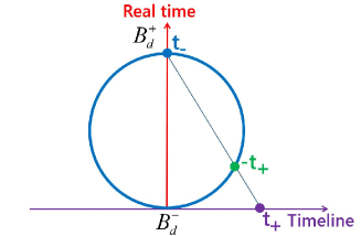
Figure 3: The stereographic projection of a point of the past $-t_{+}$ on $\mathbb{S}^{1}$ with respect to the north pole $t_{-}$ is the timeline $t_{+}$.

In $AdS_{2}$ space, the projection of past $\left(-t_{+}\right)$ concerning $t_{-}$, takes place on the timeline. The geometry of time in the black hole is represented by the sphere $\mathbb{S}^{1}$.In this case, all the points passed on the timeline, are recorded on the memory of $\mathbb{S}^{1}$. This implies that the black hole information of time is summed up in $\mathbb{S}^{1}$, which is equivalent to the time over the event horizon [42].

4.2 Time evolution in two CFTs black hole

In what follows we will divide the bulk geometry in two $AdS_{\left(+\right)d+1}$ and $AdS_{\left(-\right)d+1}$, which corresponds to the two bulk metrics (2.12), and $CFT_{d+}=B_{d}^{+,vis},CFT_{d-}=B_{d}^{-,hid}$. Indeed, the black holes exist on $B_{d}^{+,vis}$ and the events are memorized on the $\mathbb{S}^{1}$ that exists in $B_{d}^{-,hid}$. This result is comparable with the replicas are connected by the wormholes in the quantum gravity description; proposed by Penington and al [16]. Since Eq.(2.14) represents the entanglement entropy, and if we consider the invariance of the action-entropy under a global internal (3.1). Then, the classic fields $\left(f^{-},f^{+}\right)$ are two entangled particles in quantum gravity, since we have already shown in the previous section that $f^{-}\in$ $B_{d}^{-,hid}$ and $f^{+}\in$ $B_{d}^{+,vis}$. In the framework of quantum gravity, we introduce the quantum fields: the left $F^{-}\in CFT_{d-}$ and the right $F^{+}\in CFT_{d+}$. Which means, that the particles in $CFT_{d-}$ are entangled with the particles in $CFT_{d+}$, and this also agrees with ER = EPR [43]. According to [43], the entangled particles are connected through a wormhole, i.e. the holographic projection from $f^{-}$ to $f^{+}$ is done as a wormhole. Moreover, by the pure state of $L\otimes R$ or $F^{-}\otimes F^{+}$, the information transferred from $R$ to $L$ in the form of Hawking radiation, is a result of the holographic projection of $CFT_{d-}$ on $CFT_{d+}$. The connection between $CFT_{d-}$ and $CFT_{d+}$ is the origin of the pure state of $F^{-}\otimes F^{+}$. The time evolution is upward on both sides with Hamiltonian $H=H_{+}+H_{-}$. The entanglement is represented by identifying the bifurcate horizons, and filling in the space-time with interior regions behind the horizons of the black holes [43]. To describe the eternal black hole, one can use the corresponding eigenstates: $\left|+\right\rangle$ and $\left|-\right\rangle$ by two entangled states

$$\left|\Psi_{\pm}\right\rangle\sim\left|+\right\rangle\left|-\right\rangle\pm\left|-\right\rangle\left|+\right\rangle\text{.}$$ (4.10)

Here, we point out that the process followed to find the action-entropy in Eqs.(2.13,2.14)( classical gravity) is similar to Eqs.(4.10) introduced by J. Maldacena and L. Susskind [43]. The eternal black hole is described by the entangled state:

$$\left|\Psi\right\rangle=\sum_{n}e^{-\frac{\beta E_{n}}{2}}\left|n\right\rangle_{+}\otimes\left|n\right\rangle_{-},$$ (4.11)

where $\beta$ is the inverse temperature of the black hole. The evolution in quantum mechanics with the Schrodinger picture states is

$$\left|\Psi(t)\right\rangle\equiv\sum_{n}e^{-\frac{\beta E_{n}}{2}}e^{-2iE_{n}t}\left|n\right\rangle_{+}\otimes\left|n\right\rangle_{-}.$$ (4.12)

In this last equation, we consider $t$ as a parameter labeling alternate states at a common instant. In each of these states at time $t$, there exists a projection operator $P_{t}=\left|\Psi(t)\right\rangle\left\langle\Psi(t)\right|$. According to [43], two entangled states with different values of $t$ are linked by the forward time evolution on the two sides. Note that the projection operator is expressed in terms of $\left(t=t_{-},t_{+}\right)$. We assume that the system of two entangled states is formed by the state $\left|\Psi_{\pm}\right\rangle$ which depends on time $t_{\pm}$.

$$\left|\Psi_{\pm}\right\rangle=\left|\Psi_{\pm}\left(t_{\pm}\right)\right\rangle.$$ (4.13)

This approach shows that $\left|\Psi_{+}\right\rangle$ the live state in $B_{d}^{+,vis}$, on the other hand the state $\left|\Psi_{-}\right\rangle$ exists in $B_{d}^{-,hid}$. We claim that we should think that the projection of time $t_{-}$ to $t_{+}$, creates entanglement between states $\left|\Psi_{-}\right\rangle$ and $\left|\Psi_{+}\right\rangle$.

$$P_{t,n}\sim e^{2\left(-\frac{\beta}{4}-it\right)E_{n}}.$$ (4.14)

We compare this last equation with Eq.(4.9), one can obtain

$$t_{-}=-\frac{\beta}{4}\text{ \ \ \ \ \ , \ \ \ \ \ }P_{t,n}\sim e^{2zE_{n}}.$$ (4.15)

We remark that $P_{t,n}$ depends on the extra-dimensional coordinate $z$. This shows that the evolution of states corresponds to the path $z$ in the bulk. Using the last equation with Eq.(4.8), we find a value of $t_{-}$ very close to that found by [43] for a stationarity solution of the generalized entropy (with a small horizon).

5 Stereographic projection of time

Here, instead of working on one real-time, we take a set of real temporal dimensions $\mathbf{t}_{-}^{d-1}$ on $B_{d}^{-,hid}$. We will study the holographic projection from the base $(\mathbf{t}_{-}^{d-1},t_{+})$ in the full bulk $M_{d+1}$. Let us now a time sphere $\mathbb{S}^{d-2}$ by a topological subspace of dimension $d-1$, defined by

$$\mathbb{S}^{d-2}=\left\{(t_{-}^{1},t_{-}^{2},...,t_{-}^{d-1})\in R^{d-1};\sum_{k=1}^{d-1}\left(t_{-}^{k}\right)^{2}=1\right\}.$$ (5.1)

We define two poles on $\mathbb{S}^{d-2}$: the north pole of point $N=(0,...,0,1)$ and the south pole of point $S=(0,...,0,-1)$. The sphere can be covered by two stereographic parametrizations; the first open which covers the northern part of the sphere by the application $\varphi_{N}=\varphi_{-}:\mathbb{S}^{d-2}-\left\{N\right\}\longrightarrow R^{d-2}$. The second open which covers the southern part of the sphere by the stereographic projection $\varphi_{S}=\varphi_{+}:\mathbb{S}^{d-2}-\left\{S\right\}\longrightarrow R^{d-2}$:

$$\varphi_{\pm}\left(t_{-}^{1},...,t_{-}^{d-1}\right)=\left(\frac{t_{-}^{1}}{1\pm kt_{-}^{d-1}},...,\frac{t_{-}^{d-2}}{1\pm kt_{-}^{d-1}}\right),$$ (5.2)

where $k$ is a constant. This result is the generalization of the expression found by A. Almheiri and al. [43] when the extremize the generalized entropy in the $\partial^{+}$ direction is zero. Such as $t_{+}\equiv\frac{t_{-}^{1}}{1-kt_{-}^{d-1}}$, in the context of the quantum extremal surface. This shows that the choice of $\varphi_{-}$ will be preferable, i.e. the stereographic projection of time, defined by a transformation of a time sphere on $B_{d}^{-,hid}$, towards the timeline on the flat Minkowski spacetime $R^{1,d-1}\equiv$ $B_{d}^{+,vis}$. We have

$$\varphi_{-}\left(\mathbf{t}_{-}^{k},t_{-}^{d-1}\right)=\frac{\mathbf{t}_{-}^{k}}{1-kt_{-}^{d-1}}\text{ \ \ }1\preceq k\preceq d-2.$$ (5.3)

This equation is more general which presents all the holographic times $t_{+}^{k}=\varphi_{-}\left(\mathbf{t}_{-}^{k},t_{-}^{d-1}\right)$ $1\preceq k\preceq d-2$ , by the stereographic projection.

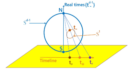
Figure 4: The stereographic projection of $\ \mathbb{S}^{d-1}$ onto the plane $\mathbb{R}^{d-1}$. The projection of a sphere $\mathbb{S}^{1}\subset\mathbb{S}^{d-1}$ on the on the timeline, creates a holographic time $t_{+}$ between the past $t_{P}$ and the future $t_{F}$.  

Next, we choose $d=4$. From Eq.(5.3) we obtain two holographic times on $B_{4}^{+,vis}$ ( or $CFT_{4}$)

$$t_{+}^{1}t_{-}^{2}=t_{-}^{1}t_{+}^{2}.$$ (5.4)

We can explain the presence of two times in $B_{4}^{+,vis}$ in two approaches:
Approach 1: Since the bulk (ex: $M_{5}=AdS_{5\text{ }}$) is described by two metrics (2.12), and one of these metrics describes geometry $M_{+5}$ surround on $B_{4}^{+,vis}=CFT_{+4}$. This shows that there is a time devoted to $AdS_{+5\text{ }}$ and another time describes $CFT_{+4}$. We suggest that $t_{+}^{1}$ and $t_{+}^{2}$ describe $CFT_{+4}$ and $AdS_{+5}$, respectively. And $t_{-}^{1}$ and $t_{-}^{2}$ describe the hidden $CFT_{-4}$ and the hidden $AdS_{-5}$, respectively. This means the $AdS$ geometry (quantum gravity) provided a time base different from the time described $CFT$ geometry ( quantum fields), i.e. $AdS_{+5}\left(t_{+}^{2}\right)/CFT_{+4}\left(t_{+}^{1}\right)$.
Approach 2: in our model, we studied $f(R)$ gravity (classical gravity), and we added to this gravity the holographic entanglement (quantum theory). Since the classical gravity described by the action (2.2) exists in $M_{5}$ and the quantum gravity described by the EE (2.3) exists in $B_{4}^{+,vis}$. We may assume that the time $t_{+}^{2}$ on classical gravity is different from time $t_{+}^{1}$ on quantum gravity.

6 Quantum time vs classical time

Now let’s focus on the second approach. If $t_{+}^{1}=t_{+}^{2}$, the gravity will be both quantum and classical. In section 4, we have used only the time $t_{+}^{1}=t_{+}^{2}$ to determine the stereographic projection for $AdS_{2}$ geometry. Which shows that the quantum-classical nature of gravity (mixed states) in a black hole. When $t_{+}^{1}\neq t_{+}^{2}$, the quantum gravity (QG) will be different from the classical gravity (CG). In this case, we propose that $t_{+}^{1}\neq t_{+}^{2}$ be valid for all regions except for singularities (black hole, …).

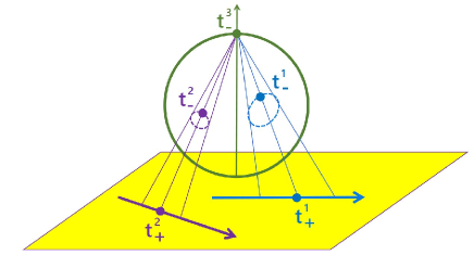
Figure 5: Approach 2: with respect to the pole $t_{-}^{3}$, there is a possibility that $t_{-}^{1}\neq t_{-}^{2}$, which generates a difference between quantum time $t_{+}^{1}$ and classical time $t_{+}^{2}$.

We have chosen to study gravitation first because the relativity of time depends on gravitational potential. We emphasize that according to special relativity, a time interval between two events measured in any inertial frame of reference is always greater than the time interval measured in the moving frame of reference relative to the first or to the highest gravitational potential. If there is a difference between the classical and the quantum time, therefore, the gravity is separated into two scales. Because we will have two gravitational potentials: $\Phi^{1}\left(t_{+}^{1}\right)$ and $\Phi^{2}\left(t_{+}^{2}\right)$. To explain this difference, we must take into account the difference between the classical scale and the quantum scale: Suppose if the solar system were small enough to reach the size of atoms. This reduction needs a period of time, this period of time is the difference between the classical and the quantum time. If this assumption is correct then the reduction is not done instantaneously. This means that we will always have in the context of special relativity even if $t_{+}^{1}\neq t_{+}^{2}$.
In the case where the classical gravity is stronger than quantum gravity ($\Phi^{CG}\left(t_{+}^{2}\right)\succ\Phi^{QG}\left(t_{+}^{1}\right)$ ); classical time goes faster than quantum time, i.e. that there is an activity on the microscopic scale compared to our scale. This concept destroys the knowledge of the quantum state $\left|\Psi_{+}\right\rangle$ at time $t_{+}^{2}$ precisely.

Maybe the idea of the difference between classical and quantum time, is the solution of the problems of passage between the two scales. We have for example the problem of $\Lambda$CDM. The dark energy density $\rho_{\Lambda}$ calculated by $\Lambda$CDM is different between the vacuum density $\rho_{vac}$ calculated by quantum field theory: $\rho_{vac}/\rho_{\Lambda}\approx 10^{121}$.

7 Conclusion

In this work, we have studied the holographic entanglement in $f(R)$ gravity. We have shown that the action is a dual of the entropy in the holographic point of view. Therefore, we have obtained a more general form of $f(R)$ gravity according to our model, which agree exactly with most choices of $f(R)$ gravity in the literature. We have shown $f(R)$ gravity in Kruskal–Szekeres coordinates, and can verifie the Lagrangian is invariant under a new general symmetry. This symmetry describe directly the geometry of the bulk manifold $M_{d+1}$. We have compared this geometry with Randall-Sundrum model and we have shown that the conformal time is a holographic projection of the hidden $d$-brane on the visible $d$-brane. On the other hand, the holographic projection of time from the hidden $3$-brane to the visible $3$-brane, creates a time $t_{+}^{1}$ which is different from the time $t_{+}^{2}$ of the bulk surrounding the visible $3$-brane. This aspect, shows us why there is a big difference between the time in quantum gravity and the time in classical gravity.

References

- [1] Sotiriou, T. P., & Faraoni, V. (2010). f (R) theories of gravity. Reviews of Modern Physics, 82(1), 451.
- [2] Gu, B. M., Liu, Y. X., & Zhong, Y. (2018). Stable Palatini f (R) braneworld. Physical Review D, 98(2), 024027.
- [3] Li, M. (2004). A model of holographic dark energy. Physics Letters B, 603(1-2), 1-5.
- [4] Hawking, S. W. (1974). Black hole explosions?. Nature, 248(5443), 30-31.
- [5] Mathur, S. D. (2009). The information paradox: a pedagogical introduction. Classical and Quantum Gravity, 26(22), 224001.
- [6] Penington, G. (2020). Entanglement wedge reconstruction and the information paradox. Journal of High Energy Physics, 2020(9), 1-84.
- [7] Penington, G., Shenker, S. H., Stanford, D., & Yang, Z. (2019). Replica wormholes and the black hole interior. arXiv preprint arXiv:1911.11977.
- [8] Almheiri, A., Hartman, T., Maldacena, J., Shaghoulian, E., & Tajdini, A. (2020). Replica wormholes and the entropy of Hawking radiation. arXiv preprint arXiv:1911.12333.
- [9] Amoretti, A., Areán, D., Goutéraux, B., & Musso, D. (2018). Effective holographic theory of charge density waves. Physical Review D, 97(8), 086017.
- [10] Nakayama, Y. (2019). Holographic dual of conformal field theories with very special deformations. Physical Review D, 100(8), 086011.
- [11] Bekenstein, J. D. (1973). Black holes and entropy. Physical Review D, 7(8), 2333.
- [12] Nishioka, T., Ryu, S., & Takayanagi, T. (2009). Holographic entanglement entropy: an overview. Journal of Physics A: Mathematical and Theoretical, 42(50), 504008.
- [13] Maldacena, J. (1999). The large-N limit of superconformal field theories and supergravity. International journal of theoretical physics, 38(4), 1113-1133.
- [14] Ryu, S., & Takayanagi, T. (2006). Aspects of holographic entanglement entropy. Journal of High Energy Physics, 2006(08), 045.
- [15] Pourhasan, R. (2014). Spacetime entanglement with gravity. Journal of High Energy Physics, 2014(6), 4.
- [16] Bousso, R., & Wildenhain, E. (2020). Gravityensemble duality. Physical Review D, 102(6), 066005.
- [17] Almheiri, A., Engelhardt, N., Marolf, D., & Maxfield, H. (2019). The entropy of bulk quantum fields and the entanglement wedge of an evaporating black hole. Journal of High Energy Physics, 2019(12), 63.
- [18] Haehl, F. M., Hartman, T., Marolf, D., Maxfield, H., & Rangamani, M. (2015). Topological aspects of generalized gravitational entropy. Journal of High Energy Physics, 2015(5), 23.
- [19] Dong, X. (2014). Holographic entanglement entropy for general higher derivative gravity. Journal of High Energy Physics, 2014(1), 44.
- [20] Bousder, M., Sakhi, Z., & Bennai, M. (2020). A new unified model of dark matter and dark energy in 5-dimensional gravity. International Journal of Geometric Methods in Modern Physics, 17(13), 2050183.
- [21] Nojiri, S. I., & Odintsov, S. D. (2007). Modified gravity as an alternative for CDM cosmology. Journal of Physics A: Mathematical and Theoretical, 40(25), 6725.
- [22] Setare, M. R. (2008). Holographic modified gravity. International Journal of Modern Physics D, 17(12), 2219-2228.
- [23] Nojiri, S. I., & Odintsov, S. D. (2007). Unifying inflation with CDM epoch in modified gravity consistent with Solar System tests. Physics Letters B, 657(4-5), 238-245.
- [24] Starobinsky, A. A. (1980). A new type of isotropic cosmological models without singularity. Physics Letters B, 91(1), 99-102.
- [25] Seahra, S. S., & Wesson, P. S. (2003). Universes encircling five-dimensional black holes. Journal of Mathematical Physics, 44(12), 5664-5680.
- [26] Mitra, A. (1999). Kruskal coordinates and mass of Schwarzschild black holes. arXiv preprint astro-ph/9904162.
- [27] Flanagan, E. E. (2004). Palatini form of gravity. Physical review letters, 92(7), 071101.
- [28] Amendola, L., Polarski, D., & Tsujikawa, S. (2007). Are dark energy models cosmologically viable?. Physical revie w letters, 98(13), 131302.
- [29] Nakamura, S., Ooguri, H., & Park, C. S. (2010). Gravity dual of spatially modulated phase. Physical Review D, 81(4), 044018.
- [30] Lieb, E. H., & Ruskai, M. B. (2002). A Fundamental Property of Quantum-Mechanical Entropy. In Inequalities (pp. 59-61). Springer, Berlin, Heidelberg.
- [31] Narain, G., & Anishetty, R. (2013). Charge renormalization due to graviton loops. Journal of High Energy Physics, 2013(7), 106.
- [32] Randall, L., & Sundrum, R. (1999). Large mass hierarchy from a small extra dimension. Physical review letters, 83(17), 3370.
- [33] Nishioka, T., & Takayanagi, T. (2007). AdS bubbles, entropy and closed string tachyons. Journal of High Energy Physics, 2007(01), 090.
- [34] Boulanger, N., & Hohm, O. (2008). Nonlinear parent action and dual gravity. Physical Review D, 78(6), 064027.
- [35] de Haro, S. (2009). Dual gravitons in and the holographic Cotton tensor. Journal of High Energy Physics, 2009(01), 042.
- [36] Henneaux, M., Lekeu, V., & Leonard, A. (2019). A note on the double dual graviton. Journal of Physics A: Mathematical and Theoretical, 53(1), 014002.
- [37] Garcia-Compean, H., Obregon, O., Ramirez, C., & Sabido, M. (2003). Noncommutative self-dual gravity. Physical Review D, 68(4), 044015.
- [38] Maldacena, J., Stanford, D., & Yang, Z. (2016). Conformal symmetry and its breaking in two-dimensional nearly anti-de Sitter space. Progress of Theoretical and Experimental Physics, 2016(12).
- [39] Engelsöy, J., Mertens, T. G., & Verlinde, H. (2016). An investigation of AdS 2 backreaction and holography. Journal of High Energy Physics, 2016(7), 139.
- [40] Almheiri, A., & Kang, B. (2016). Conformal symmetry breaking and thermodynamics of near-extremal black holes. Journal of High Energy Physics, 2016(10), 52.
- [41] Faulkner, T., Leigh, R. G., Parrikar, O., & Wang, H. (2016). Modular Hamiltonians for deformed half-spaces and the averaged null energy condition. Journal of High Energy Physics, 2016(9), 38.
- [42] Frolov, V. P. (2014). Information loss problem and a ‘black hole’model with a closed apparent horizon. Journal of High Energy Physics, 2014(5), 49.
- [43] Maldacena, J., & Susskind, L. (2013). Cool horizons for entangled black holes. Fortschritte der Physik, 61(9), 781-811.