Anti-Poiseuille flow in neutral graphene

Abstract

Hydrodynamic flow of charge carriers in graphene is an energy flow unlike the usual mass flow in conventional fluids. In neutral graphene, the energy flow is decoupled from the electric current, making it difficult to observe the hydrodynamic effects and measure the viscosity of the electronic fluid by means of electric current measurements. In particular, we show that the hallmark Poiseuille flow in a narrow channel cannot be driven by the electric field irrespective of boundary conditions at the channel edges. Nevertheless one can observe nonuniform current densities similarly to the case of the well-known ballistic-diffusive crossover. The standard diffusive behavior with the uniform current density across the channel is achieved under the assumptions of specular scattering on the channel boundaries. This flow can also be made nonuniform by applying weak magnetic fields. In this case, the curvature of the current density profile is determined by the quasiparticle recombination processes dominated by the disorder-assisted electron-phonon scattering – the so-called supercollisions.

Electronic hydrodynamics has attracted substantial experimental and theoretical attention in recent years [1, 2, 3]. Hydrodynamic flows in two-dimensional (2D) materials can now be observed directly using several imaging techniques [4, 5, 6, 7, 8, 9, 10, 11, 12, 13, 14]. Two of these experiments [10, 11] were focusing on the Poiseuille flow, the simplest manifestation of viscous hydrodynamics in conventional fluids [15].

The Poiseuille flow [16, 17, 15] is a pressure-induced flow in a pipe or between parallel plates. The latter is equivalent to a 2D flow in a narrow channel (with the length $L$ much greater than the width $W$). In the middle of the channel (away from both of its ends) the flow velocity is directed along the channel and depends only on the transverse coordinate. In that case, the hydrodynamic equations admit a simple solution with the parabolic velocity profile and the flow rate (discharge) that is proportional to the third power of the channel width (for a three-dimensional flow through a pipe – the fourth power of the radius, which is especially important in hematology [18]).

The possibility for an electronic system to exhibit the Poiseuille flow in a narrow wire was first pointed out by Gurzhi [19, 20, 21]. Recently, similar behavior has been a subject of intense theoretical [22, 23, 24, 25, 26, 27, 28, 29, 30, 31, 32, 33] and experimental [22, 10, 11, 12, 34, 35, 36, 13, 37, 38, 39, 40, 41, 42, 43, 44] research in the context of electronic transport in high-mobility 2D materials. In contrast to conventional fluids, the electronic flow is affected not only by viscous effects, but also by weak disorder scattering and is characterized by a typical length scale known as the Gurzhi length [26, 27, 28, 29, 33]

$$\ell_{G}=\sqrt{\nu\tau_{\rm dis}}.$$ (1)

Here $\nu$ is the kinematic viscosity [15, 3, 45, 46, 47] and $\tau_{\rm dis}$ is the disorder mean free time. The resulting current profile is given by the catenary curve approaching the parabola in the limit ${\ell_{G}\gg{W}}$.

Nonuniform hydrodynamic flow in a narrow channel has to be contrasted with a conventional ballistic flow that in the case of realistic boundary conditions [10, 48] can also be nonuniform. Assuming rough edges, where electrons scatter off in all directions with equal probability (“diffusive scattering”), bulk impurity scattering competes with boundary effects leading to a ballistic-diffusive crossover. If the mean free path is much smaller than the channel width, $\ell_{\rm dis}\ll W$, then the electric current density is uniform, except for the small regions close to the edges. Reducing the channel width leads to the appearance of a curved current profile that is visually similar to the Poiseuille flow (with the maximum curvature corresponding to both length scales being of the same order of magnitude). In doped graphene this was observed in the recent imaging experiment [10].

Physics of neutral graphene [11, 49, 50] is more intricate. Here the electronic system is nondegenerate and both graphene bands contribute to transport on equal footing. Due to linearity of the Dirac spectrum, the Auger processes are kinematically suppressed and to the leading approximation the number of particles in each band is conserved independently [2, 3, 51, 52]. Another consequence of the peculiar kinematics of Dirac fermions in graphene is the so-called “collinear scattering singularity” [53, 54, 55, 56, 52, 57, 58, 59] that gives rise to the “three-mode approximation” allowing one to solve the kinetic equation and derive the hydrodynamic theory [59, 60, 61]. The key feature of the resulting description is that the hydrodynamic flow in graphene is the flow of energy rather than mass in conventional fluids or charge in Ohmic conductors [2, 3, 60, 61]. Precisely at charge neutrality and in the absence of external magnetic field, the hydrodynamic energy flow is completely decoupled from the electric current. In an infinite system the latter exhibits usual Ohmic behavior with the dominant contribution to the mean free path coming from electron-electron interaction [50, 55, 54, 60, 62, 61, 63]. It is then reasonable to expect that in a narrow channel this current should exhibit the above ballistic-diffusive crossover with the only difference being the microscopic nature of the mean free path.

Hydrodynamic flows in neutral graphene were recently studied experimentally with the help of nanoscale magnetic imaging [11]. The authors reported measurements of inhomogeneous electric current density interpreting them in terms of the Poiseuille flow. Assuming that the curvature of the current density profile was determined by viscosity, the authors proceeded to extract the shear viscosity in graphene at and close to charge neutrality. The resulting values appeared to be in a surprisingly good agreement with the theoretical calculations of Ref. [47].

What exactly is the Poiseuille flow and can it be used as a hallmark of hydrodynamic behavior? The Poiseuille flow is a particular solution to the Navier-Stokes equation [15] in the case where a viscous, incompressible fluid is constrained by (straight and infinitely long) stationary boundaries. The problem is usually solved under the assumption of the so-called no-slip boundary conditions, i.e. the vanishing flow velocity at the boundaries. Then the Navier-Stokes equation becomes an ordinary second-order differential equation yielding the standard parabolic velocity profile. The solution can be extended to the case of more general Maxwell’s boundary conditions [64] with a finite slip length [65]. The limit of the infinite slip length however (i.e., with no-stress boundary conditions) does not admit any solutions for the Poiseuille problem. In other words: a pressure-induced viscous flow in a pipe cannot be homogeneous. On the contrary, an inviscid fluid is described by the Euler equation [15], which is a nonlinear, first-order differential equation. As such, it does not require boundary conditions on the longitudinal (along the boundary) component of the velocity and allows for homogeneous solutions. Hence, the Poiseuille flow can be used as a hallmark of viscosity.

Adapting the above arguments to electronic transport is straightforward for single-band, Fermi-liquid-like systems, such as doped graphene. Here all physical quantities are determined by the Fermi energy, all macroscopic currents are physically equivalent and can be represented by a single vector quantity, the velocity $\boldsymbol{u}$. In the “hydrodynamic regime”, i.e., if the electron-electron interaction is the dominant scattering mechanism in the problem, $\ell_{ee}\ll\ell_{\rm dis},\ell_{e-ph},W$ (in the self-evident notation), $\boldsymbol{u}$ obeys a Navier-Stokes-like equation [3, 2, 61] and may exhibit a Poiseuille-like behavior in a channel [10].

Electronic hydrodynamics in graphene – In a two-band system the situation is more involved. An out-of-equilibrium (current-carrying) state may be characterized either by the chemical potentials $\mu_{\pm}$ of each band, or by their linear combinations [51, 61]

$$\mu=(\mu_{+}\!+\!\mu_{-})/2,\qquad\mu_{I}=(\mu_{+}\!-\!\mu_{-})/2,$$ (2a)

conjugate to the charge and imbalance densities

$$n=n_{+}-n_{-},\qquad n_{I}=n_{+}+n_{-}.$$ (2b)

In equilibrium ${\mu_{I}=0}$. Although macroscopic currents are no longer equivalent [59, 60, 51, 61], one can still introduce the hydrodynamic velocity associating it with one (nearly) conserved current, namely the momentum flux. In the case of linear spectrum, the momentum flux is equivalent to the energy current. As a result, the electric ($\boldsymbol{j}$), quasiparticle (or “imbalance”, $\boldsymbol{j}_{I}$), and energy ($\boldsymbol{j}_{E}$) currents in graphene can be defined as [2, 3, 61]

$$\boldsymbol{j}=n\boldsymbol{u}\!+\!\delta\boldsymbol{j},\quad\boldsymbol{j}_{I}=n_{I}\boldsymbol{u}\!+\!\delta\boldsymbol{j}_{I},\quad\boldsymbol{j}_{E}={\cal W}\boldsymbol{u},$$ (3)

where ${\cal W}$ is the enthalpy density and $\delta\boldsymbol{j}$ and $\delta\boldsymbol{j}_{I}$ are the dissipative corrections, see Eqs. (7) below and the Appendix. In the degenerate limit ${\mu\gg{T}}$ the dissipative corrections vanish [61, 63] justifying the applicability of the above single-band picture to doped graphene. At charge neutrality ${n=0}$, the electric and energy currents in Eq. (3) appear to be decoupled [61].

The quasiparticle currents $\boldsymbol{j}$ and $\boldsymbol{j}_{I}$ satisfy the continuity equations [2, 3, 61, 66]

$$\partial_{t}n+\boldsymbol{\nabla}\!\cdot\!\boldsymbol{j}=0,$$ (4a)

$$\partial_{t}n_{I}+\boldsymbol{\nabla}\!\cdot\!\boldsymbol{j}_{I}=-\frac{n_{I}\!-\!n_{I,0}}{\tau_{R}}=-\frac{12\ln 2}{\pi^{2}}\frac{n_{I,0}\mu_{I}}{T\tau_{R}},$$ (4b)

where $${n_{I,0}=\pi{T}^{2}/(3v_{g}^{2})} \mu_{I}=0 \tau_{R} \boldsymbol{u}$$ is the equilibrium value of the total quasiparticle density (i.e., at ) and is the recombination time [67, 66]. The hydrodynamic velocity satisfies the generalized Navier-Stokes equation [61]

$$\!\!\!\!\!\!{\cal W}(\partial_{t}+\boldsymbol{u}\!\cdot\!\boldsymbol{\nabla})\boldsymbol{u}+v_{g}^{2}\boldsymbol{\nabla}P+\boldsymbol{u}\partial_{t}P+e(\boldsymbol{E}\!\cdot\!\boldsymbol{j})\boldsymbol{u}=$$ (4c)

$$=v_{g}^{2}\left[\eta\Delta\boldsymbol{u}+en\boldsymbol{E}+\frac{e}{c}\boldsymbol{j}\!\times\!\boldsymbol{B}\right]-{\cal W}\boldsymbol{u}/\tau_{{\rm dis}},$$

where $$P \eta$$ and are the thermodynamic pressure and shear viscosity. The full hydrodynamic equations [51, 68] also includes the thermal transport equation [66]

$$T\left[\frac{\partial s}{\partial t}+\boldsymbol{\nabla}\!\cdot\!\left(s\boldsymbol{u}-\delta\boldsymbol{j}\frac{\mu}{T}-\delta\boldsymbol{j}_{I}\frac{\mu_{I}}{T}\right)\right]=$$ (4d)

$$\qquad\qquad=\delta\boldsymbol{j}\!\cdot\!\left[e\boldsymbol{E}\!+\!\frac{e}{c}\boldsymbol{u}\!\times\!\boldsymbol{B}\!-\!T\boldsymbol{\nabla}\frac{\mu}{T}\right]-T\delta\boldsymbol{j}_{I}\!\cdot\!\boldsymbol{\nabla}\frac{\mu_{I}}{T}$$

$$\qquad\qquad\qquad+\frac{\eta}{2}\left(\nabla_{\alpha}u_{\beta}\!+\!\nabla_{\beta}u_{\alpha}\!-\!\delta_{\alpha\beta}\boldsymbol{\nabla}\!\cdot\!\boldsymbol{u}\right)^{2}$$

$$\qquad\qquad\qquad-\frac{n_{E}\!-\!n_{E,0}}{\tau_{RE}}+\mu_{I}\frac{n_{I}\!-\!n_{I,0}}{\tau_{R}}+\frac{{\cal W}\boldsymbol{u}^{2}}{v_{g}^{2}\tau_{\rm dis}},$$

which is typically used in hydrodynamics [15] instead of the continuity equation representing energy conservation. Here $n_{E,0}$ denotes the equilibrium value of the energy density similarly to $n_{I,0}$ (i.e., at ${\mu_{I}=0}$) and $\tau_{RE}$ is the energy relaxation time (due to, e.g., supercollisions [66]). The last three terms in Eq. (4d) represent energy relaxation, entropy increase due to quasiparticle recombination, and local heating due to impurity scattering.

Consider now linear response transport in the channel geometry (see Refs. [10, 11] for experimental realization) at charge neutrality (${n=0}$) in the steady state. Linearizing the hydrodynamic equations (4), we obtain [66]

$$\boldsymbol{\nabla}\!\cdot\!\delta\boldsymbol{j}=0,$$ (5a)

$$n_{I,0}\boldsymbol{\nabla}\!\cdot\!\boldsymbol{u}+\boldsymbol{\nabla}\!\cdot\!\delta\boldsymbol{j}_{I}=-(12\ln 2/\pi^{2})n_{I,0}\mu_{I}/(T\tau_{R}),$$ (5b)

$$\boldsymbol{\nabla}\delta P=\eta\Delta\boldsymbol{u}+(e/c)\delta\boldsymbol{j}\!\times\!\boldsymbol{B}-3P\boldsymbol{u}/(v_{g}^{2}\tau_{{\rm dis}}),$$ (5c)

$$3P\boldsymbol{\nabla}\!\cdot\!\boldsymbol{u}=-2\delta{P}/\tau_{RE},$$ (5d)

where we have used the “equation of state” [61]

$${\cal W}=3{P}=3{n}_{E}/2.$$

Here we follow the standard approach [15] where the thermodynamic quantities are replaced by the corresponding equilibrium functions of the hydrodynamic variables. Equations (5) should be solved for the unknowns $\boldsymbol{u}$, $\mu_{I}$, and $\delta P$ keeping the rest of the quantities, e.g., $n_{I,0}$, $P$, and $T$, constant (the dissipative corrections $\delta\boldsymbol{j}$, $\delta\boldsymbol{j}_{I}$ are specified below).

At charge neutrality, the electric field vanishes from the linearized Navier-Stokes equation (5c) and hence cannot drive a hydrodynamic flow.

Channel geometry: absence of the Poiseuille flow in neutral graphene – The channel geometry can be modeled by an “infinite” strip (i.e., with the length of the sample much greater than its width). Transport measurements are assumed to be performed in the two-terminal scheme [10, 11] with the leads placed at the far away ends of the channel. In the middle of the sample, the electric current is flowing along the channel and all physical quantities are independent of the longitudinal coordinate $x$ (this is not true in small regions close to the leads at the ends of the channel). At ${n=0}$, the electric current is given by the dissipative correction ($y$ is the transverse coordinate)

$$\boldsymbol{j}=\delta\boldsymbol{j}=\delta j_{x}(y)\boldsymbol{e}_{x},$$ (6a)

automatically satisfying the continuity equation (5a). The pressure is also a function of $$y$$

$$\delta P=\delta P(y)\quad\Rightarrow\quad\boldsymbol{\nabla}\delta P=\frac{\partial\delta P}{\partial y}\boldsymbol{e}_{y},$$ (6b)

and similarly

$$\mu_{I}=\mu_{I}(y)\quad\Rightarrow\quad\boldsymbol{\nabla}\mu_{I}=\frac{\partial\mu_{I}}{\partial y}\boldsymbol{e}_{y}.$$ (6c)

Projecting the Navier-Stokes equation (5c) onto the longitudinal direction, we find

$$\eta\frac{\partial^{2}u_{x}}{\partial y^{2}}=\frac{3Pu_{x}}{v_{g}^{2}\tau_{\rm dis}}\quad\Rightarrow\quad u_{x}=0.$$ (6d)

This is a homogeneous equation that yields the trivial solution $$u_{x}=0$$ for either the no-slip or no-stress boundary conditions. As a result,

$$\boldsymbol{u}=u_{y}(y)\boldsymbol{e}_{y}\quad\Rightarrow\quad\boldsymbol{\nabla}\!\cdot\!\boldsymbol{u}=\frac{\partial u_{y}}{\partial y}.$$ (6e)

Equations (6) represent the key difference between the usual hydrodynamic flow and electronic transport in neutral graphene. The standard Poiseuille flow is driven by the pressure gradient. In contrast, charge carriers in graphene may be driven by the electric field. At charge neutrality, the field term vanishes from the Navier-Stokes equation leading to the homogeneous equation (6d) for the longitudinal component of the velocity. In other words, in neutral graphene the Poiseuille flow cannot be driven by the electric field. Instead, one should apply a temperature gradient along the channel [in this case, the pressure gradient in Eq. (6b) will acquire an $x$-component contributing a driving term to Eq. (6d)], see also Ref. [69]. We emphasize that this result does not depend on microscopic details of carrier scattering off the channel edges.

What does this mean for the electric current? To clarify this question, we have to specify the dissipative corrections $\delta\boldsymbol{j}$ and $\delta\boldsymbol{j}_{I}$. Their general form was derived in bulk graphene in Refs. [61, 63], see also Appendix. This derivation relied on the specific form of the nonequilibrium correction to the distribution function [see Eq. (17) in the Appendix] representing a natural generalization of the usual solution to the kinetic equation in metals [70] to the two-band Dirac system in graphene. In a narrow channel, solutions to the kinetic equation should be subjected to boundary conditions [48] reflecting the nature of the electron scattering off the channel edges. Specifically at charge neutrality, the typical wavelength of Dirac quasiparticles is determined by temperature and thus is much larger than the length scale of the edge roughness that may lead to diffusive boundary scattering [48]. As a result, specular boundary conditions can be expected to adequately describe neutral graphene samples.

In the limit of specular scattering, the distribution function Eq. (17) satisfies the boundary conditions and the form of the dissipative corrections remains the same as in the bulk system. At charge neutrality, the corrections are given by

$$\delta\boldsymbol{j}=\frac{1}{e^{2}\tilde{R}}\left[e\boldsymbol{E}+\omega_{B}\boldsymbol{e}_{B}\!\times\!\left(\frac{\alpha_{1}\delta_{I}\boldsymbol{\nabla}\mu_{I}}{\tau_{\rm dis}^{-1}\!+\!\delta_{I}^{-1}\tau_{22}^{-1}}-\frac{2T\ln 2}{v_{g}^{2}}\boldsymbol{u}\right)\!\right]\!,$$ (7a)

$$\delta\boldsymbol{j}_{I}=-\frac{\delta_{I}}{\tau_{\rm dis}^{-1}\!+\!\delta_{I}^{-1}\tau_{22}^{-1}}\frac{1}{e^{2}\tilde{R}}\times$$ (7b)

$$\quad\times\!\left[\alpha_{1}\omega_{B}\boldsymbol{e}_{B}\!\times\!\boldsymbol{E}\!+\!\frac{2T\ln 2}{\pi}e^{2}R_{0}\boldsymbol{\nabla}\mu_{I}\!+\!\alpha_{1}\omega_{B}^{2}\frac{2T\ln 2}{v_{g}^{2}}\boldsymbol{u}\right]\!,$$

$$\tilde{R}=R_{0}\!+\!\alpha_{1}^{2}\delta_{I}\tilde{R}_{B}.$$ (7c)

Here $R_{0}$ [see Eq. (29)] is the zero-field bulk resistivity in neutral graphene [59, 61, 56], ${\tilde{R}_{B}\propto\omega_{B}^{2}\tau_{\rm dis}}$ is defined in Eq. (30), ${\omega_{B}=eBv_{g}^{2}/(2cT\ln 2)}$ is the generalized cyclotron frequency (at ${\mu=0}$), ${\alpha_{1}\approx 2.08}$ and ${\delta_{I}\approx 0.28}$ are detailed in Appendix ($v_{g}$ is the band velocity in graphene, $c$ is the speed of light, and $e$ is the electron charge). The parameter $\tau_{22}$ describes the integrated collision integral, see Eqs. (25). Both $\tau_{\rm dis}$ and $\tau_{22}$ are functions of the chemical potential and temperature [61, 63, 71].

At ${\boldsymbol{B}=0}$, the corrections (7) simplify. The electric current (${e\delta\boldsymbol{j}=\boldsymbol{E}/R_{0}}$) is governed by Ohmic dissipative processes and is independent of the hydrodynamic velocity. Thus, we immediately arrive at the conclusion that in the absence of magnetic field the resulting current density in neutral graphene with specular boundaries is uniform [61, 63] (in contrast to conventional hydrodynamics that does not allow for a stationary pressure-induced flow in a channel without boundary friction [15]).

Nonuniform flows in magnetic field – Now we show that even in the case of specular scattering on the channel boundaries the electric current density can be made nonuniform by applying weak external magnetic field. In the presence of the field all three macroscopic currents are entangled [59] and one may expect a nontrivial solution. The electric current is still flowing along the channel, but is accompanied by the lateral flow of quasiparticles [67, 72]. Since the latter cannot leave the sample, this flow has to vanish at both edges and (nontrivial) homogeneous solutions are no longer allowed. In the two-fluid model of compensated semimetals [72, 28, 73, 74] the nontrivial inhomogeneous solution becomes possible due to quasiparticle recombination.

Quasiparticle recombination refers to any scattering process that violates the “approximate” conservation of the number of particles in each individual band including the kinematically suppressed Auger processes, three-particle collisions, scattering by optical phonons [75, 68], and the disorder-assisted electron-phonon coupling (or “supercollisions”) [76, 77, 78, 79, 80, 66]. The resulting quasiparticle recombination is manifested by an additional term in the continuity equation (4b) for the total quasiparticle (“imbalance”) density, first established in Ref. [51] in the context of thermoelectric phenomena. Recently, recombination effects were shown to lead to linear magnetoresistance in compensated semimetals [81, 72, 73, 28], giant magnetodrag [82, 67], and giant nonlocality [83, 74].

Supercollisions involve electron-phonon scattering in a close proximity to an impurity. This is a second-order process where an electron in the upper graphene band may scatter into an empty state in the lower band while emitting a phonon and losing its momentum to the impurity. In the reverse process, the phonon can be absorbed by an electron in the lower band scattering into the upper band (while the impurity compensates the momentum mismatch). Unlike the Auger or three-particle processes, supercollisions also lead to energy relaxation [66]. Taking into account recombination without energy relaxation leads to a problem: the continuity equations for energy and imbalance densities allow only homogeneous solutions, which are incompatible with the boundary conditions at the channel edges. Here we show that energy relaxation due to supercollisions provides the missing piece of the puzzle allowing one to solve the hydrodynamic equations in graphene at charge neutrality. The solution exhibits the inhomogeneous electric current profile in neutral graphene samples with specular reflective boundaries subjected to weak magnetic field. We find that the curvature of the current profile is determined by supercollisions (by means of energy relaxation and quasiparticle recombination) rather than viscosity. A case of rough edges and the corresponding ballistic-diffusive crossover will be discussed elsewhere.

Substituting Eqs. (6) into Eqs. (7) and (5) we find five equations for five unknowns. Excluding $\delta P$, $\mu_{I}$, and $\delta j_{x}$, we are left with two equations for $u_{y}$ and $\delta j_{I,y}$. For further analysis it is convenient to express them in terms of dimensionless quantities

$$q=\frac{n_{I,0}u_{y}}{q_{0}},\quad p=\frac{\delta j_{I,y}}{q_{0}},\quad q_{0}=\frac{\omega_{B}\tau_{\rm dis}E}{e\tilde{R}},$$ (8)

in the matrix form

$$\widehat{L}\begin{pmatrix}q^{\prime\prime}\cr p^{\prime\prime}\end{pmatrix}=\widehat{M}\begin{pmatrix}q\cr p\end{pmatrix}+\begin{pmatrix}\alpha_{3}\cr p_{0}\end{pmatrix}.$$ (9)

The matrix $\widehat{L}$ comprises squares of the recombination-related length scales

$$\widehat{L}=\begin{pmatrix}\ell^{2}_{RG}-\ell^{2}_{R1}&-\ell^{2}_{R1}\cr\ell^{2}_{R2}&\ell^{2}_{R2}\end{pmatrix},$$ (10a)

$$\ell^{2}_{RG}=\frac{1}{2}\ell^{2}_{RE}+\frac{2\pi}{9\zeta(3)}\frac{\eta v_{g}^{4}\tau_{\rm dis}}{T^{3}},\quad\ell^{2}_{RE}=v_{g}^{2}\tau_{RE}\tau_{\rm dis},$$ (10b)

$$\ell^{2}_{R1}=\alpha_{1}\alpha_{3}\delta_{I}\frac{\tilde{R}_{B}}{2\tilde{R}}\ell^{2}_{R},\quad\ell^{2}_{R}=v_{g}^{2}\tau_{R}\tau_{\rm dis},$$ (10c)

$$\ell^{2}_{R2}=\delta_{I}\frac{R_{0}}{2\tilde{R}}\frac{\ell^{2}_{R}}{1\!+\!\tau_{\rm dis}/(\delta_{I}\tau_{22})},$$ (10d)

while the remaining quantities are dimensionless

$$\alpha_{3}=\frac{2\pi^{2}\ln 2}{27\zeta(3)}\approx 0.42,\quad p_{0}=\frac{\alpha_{1}\delta_{I}}{1\!+\!\tau_{\rm dis}/(\delta_{I}\tau_{22})},$$ (10e)

$$\widehat{M}=\begin{pmatrix}C_{1}&0\cr C_{2}&1\end{pmatrix},$$ (10f)

$$C_{1}=\frac{R_{0}\!+\!\delta R(B)}{\tilde{R}},\quad C_{2}=\frac{12\alpha_{1}\delta_{I}\tilde{R}_{B}\ln^{2}2}{\pi^{2}\tilde{R}}.$$ (10g)

The correction ${\delta R(B)\propto\omega_{B}^{2}\tau_{\rm dis}}$ is defined in Eq. (A).

Once Eqs. (9) are solved, we can find the electric current (6a) by substituting the solutions $q(y)$ and $p(y)$ into Eq. (7a) using Eqs. (8) and (5b). As a result, we find

$$\delta j_{x}(y)=\frac{E}{eR_{0}}\left[1+\frac{\omega_{B}^{2}\tau_{\rm dis}}{e^{2}\tilde{R}\,T}\!\left(\frac{\pi\alpha_{1}}{2\ln 2}\,p+\frac{6\ln 2}{\pi}\,q\right)\!\right]\!.$$ (11)

We reiterate, that Eq. (11) describes viscous electronic fluid in neutral graphene (in contrast to the inviscid system of carriers considered in Ref. [59]).

Anti-Poiseuille flow – Equations similar to Eq. (9) have been solved in Refs. [59, 72, 73, 28, 29] focusing on the resulting magnetoresistance. In this paper, we are interested in the spatial profile of the quasiparticle currents. Requiring the “hard-wall” boundary conditions

$$u_{y}(\pm W/2)=\delta j_{I,y}(\pm W/2)=0,$$ (12)

we find the solution to Eq. (9) in the form of the catenary curve

$$\begin{pmatrix}q\cr p\end{pmatrix}=\left[\frac{\cosh(\widehat{\cal K}y)}{\cosh(\widehat{\cal K}W/2)}-1\right]\widehat{M}^{-1}\begin{pmatrix}\alpha_{3}\cr p_{0}\end{pmatrix},$$ (13)

where

$$\widehat{\cal K}^{2}=\widehat{L}^{-1}\widehat{M}.$$

Substituting the result (13) into Eq. (11) we find the electric current profile. The analytical expression for $\delta j_{x}(y)$ contains a $y$-independent contribution inherited from the first term in Eq. (11) and the second term in Eq. (13) as well as the catenary terms describing the $y$ dependence of $q$ and $p$ from Eq. (13). Following Ref. [11], we normalize the current by its average value

$$\bar{j_{x}}=\frac{1}{W}\!\!\int\limits^{W/2}_{-W/2}\!\!dy\,\delta j_{x}(y),$$ (14)

which can be obtained by averaging the solution (13) and substituting the result into Eq. (11). Averaging of Eq. (13) can be performed in the matrix form yielding

$$\begin{pmatrix}\bar{q}\cr\bar{p}\end{pmatrix}=\left[\frac{\tanh(\widehat{\cal K}W/2)}{\widehat{\cal K}W/2}-1\right]\widehat{M}^{-1}\begin{pmatrix}\alpha_{3}\cr p_{0}\end{pmatrix}.$$ (15)

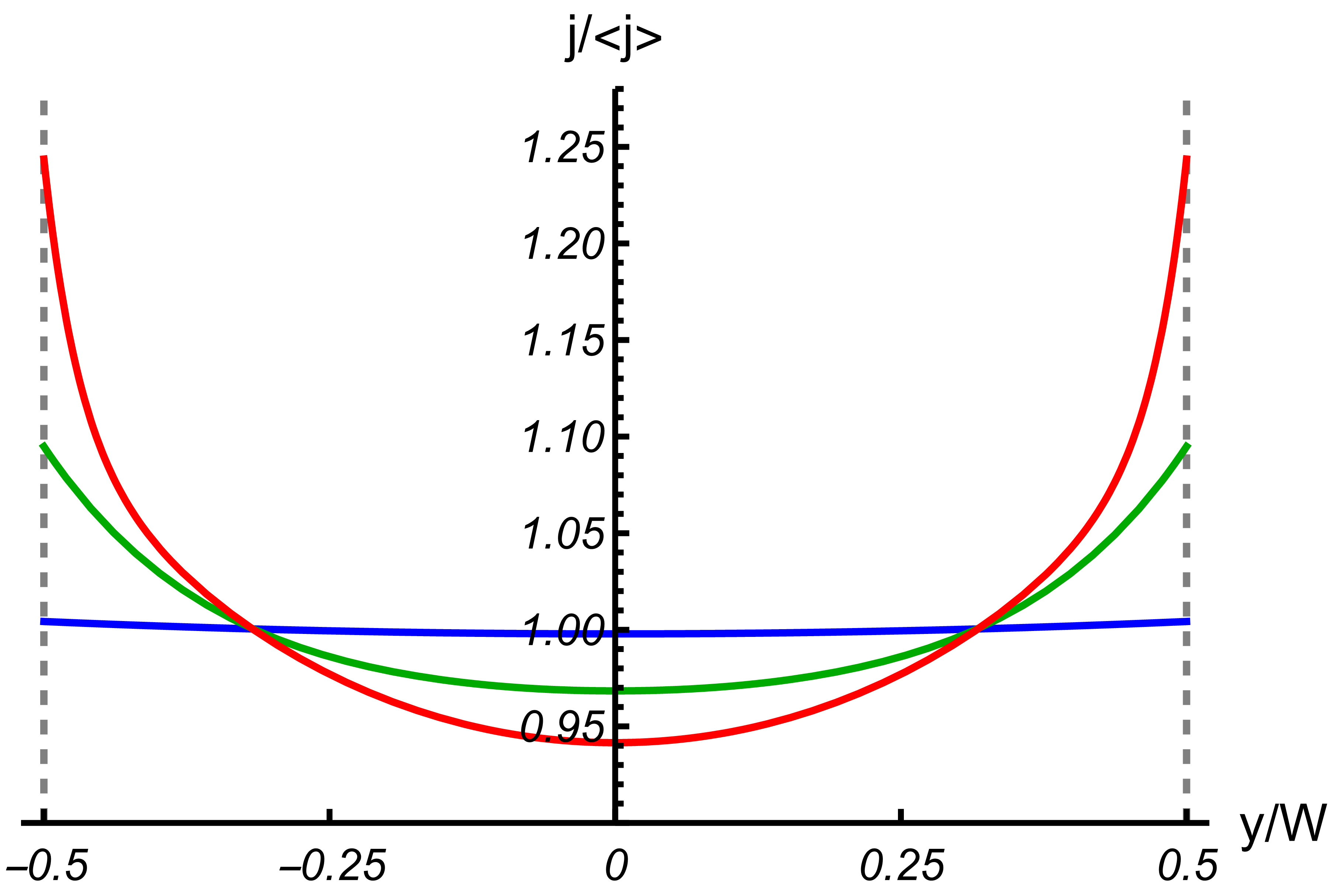
Figure 1: Catenary curves of the current density in the narrow channel Eq. (11) normalized by the averaged current density Eq. (14). The numerical results were obtained for typical parameter values (${\tau_{\rm dis}\approx 0.8}\,$THz [50], ${\alpha_{g}\approx 0.2}$ [50, 84], ${\nu\approx 0.4}\,$m${}^{2}/$s [47, 11], ${B=0.1}\,$T, ${T=250}\,$K) and correspond to three values of the channel width, ${W=0.1,\,1,\,5}\,\mu$m (blue, green, and red curves, respectively).

The resulting inhomogeneous current density is illustrated in Fig. 1. In some sense, the profile in Fig. 1 can be regarded as “anti-Poiseuille”: unlike the true Poiseuille flow, this current density exhibits a minimum in the center of the channel and is finite at the edges (in fact, there it reaches its maximum). The numerical values of the current density were obtained by using a typical experimental value ${\tau_{\rm dis}\approx 0.8}\,$THz [50], and assuming the effective coupling constant ${\alpha_{g}\approx 0.2}$ following Refs. [50, 84], temperature ${T=250}\,$K, magnetic field ${B=0.1}\,$T, and channel width ${W=1}\,\mu$m. The viscosity affects the current only through the length scale $\ell_{RG}$, see Eq. (10b). This effect is rather weak: varying the kinematic viscosity in the range ${\nu\approx 0.2-0.4}\,$m${}^{2}/$s [47] does not significantly change the results. The recombination length ${\ell_{R}\approx 2}\,\mu$m and the energy relaxation length ${\ell_{RE}\approx 5}\,\mu$m were chosen phenomenologically, using the data of Ref. [67] as a guide (see also Ref. [66] for theoretical estimates).

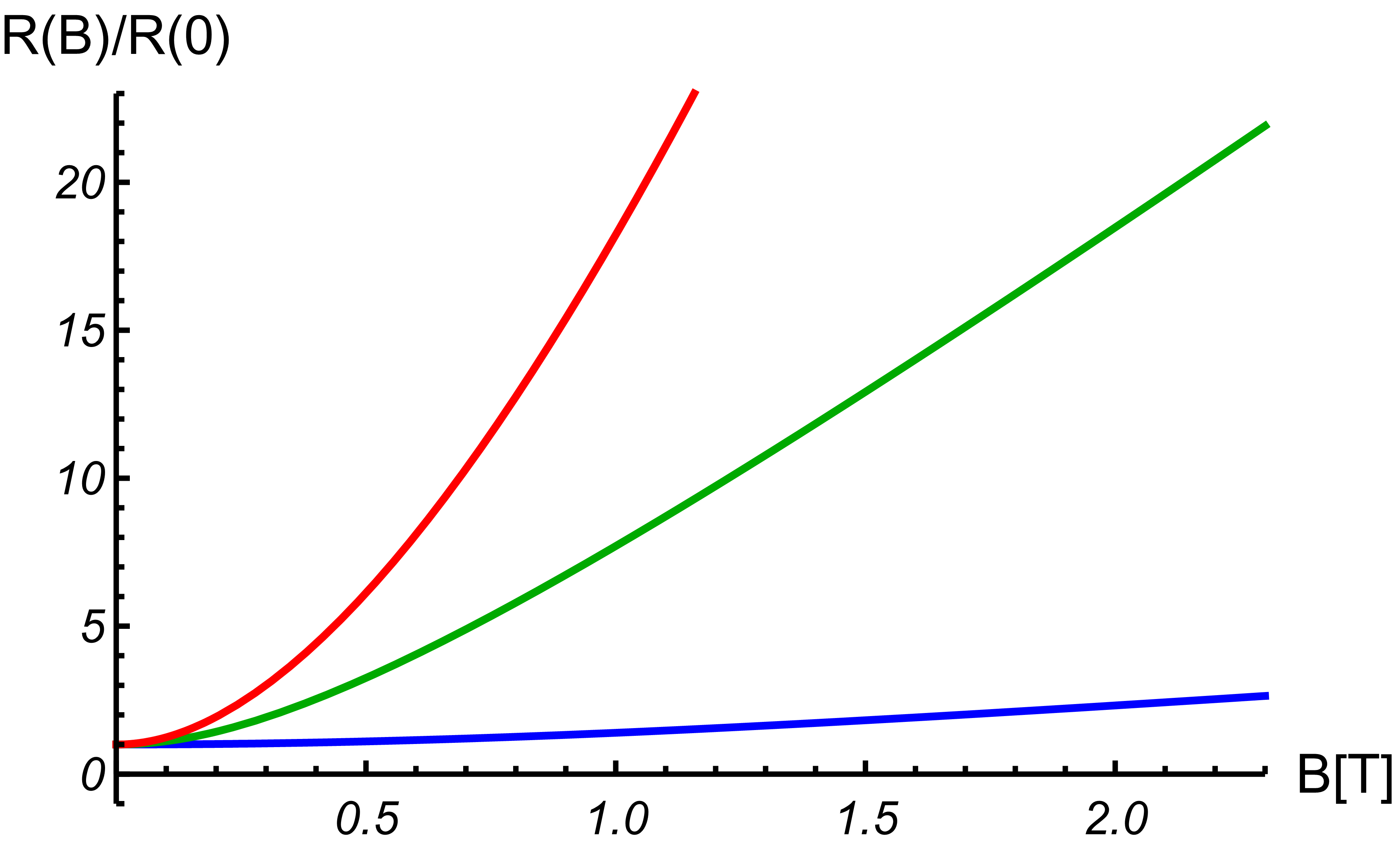
Figure 2: Magnetoresistance in the narrow channel following from Eqs. (11) and (14) normalized by the zero field resistance $R_{0}$. The numerical results were obtained for typical parameter values (${\tau_{\rm dis}\approx 0.8}\,$THz [50], ${\alpha_{g}\approx 0.2}$ [50, 84], ${\nu\approx 0.4}\,$m${}^{2}/$s [47, 11], ${B=0.1}\,$T, ${T=250}\,$K) and correspond to three values of the channel width, ${W=0.1,\,1,\,5}\,\mu$m (blue, green, and red curves, respectively).

Discussion – The results presented in this paper have to be contrasted with recent developments in the field. Most theoretical work on hydrodynamic behavior in neutral (or compensated) materials has been devoted to infinite (or bulk) systems [3, 2, 55, 56, 59, 61]. A bulk system is translationally invariant and hence the current density is uniform with the corresponding sheet resistance given by $R_{0}$. In confined geometries the resulting flow profiles are determined by the interplay of sample geometry, boundary conditions, and bulk interaction effects [85]. With respect to electron-electron interaction, three types of theories have been proposed: (i) macroscopic linear response theory of the inviscid electronic fluid [59], (ii) two-fluid hydrodynamics [72, 28, 73, 74], and (iii) viscous electronic hydrodynamics that is the subject of the present paper. The difference between the three theories can be summarized as follows. (i) Ref. [59] generalized the standard transport theory (basically the Ohm’s law) to graphene close to charge neutrality, where electron-electron interaction contributes to resistivity directly due to lack of Galilean invariance. The resulting theory comprises three (algebraic) equations for three macroscopic currents and does not take into account any possible viscous effects. (ii) The two-fluid model of Ref. [28] assumes that the electron and hole subsystems (i.e. quasiparticles in two different bands) are independently equilibrated and form two separate fluids, while the electron-hole scattering leads to a (weak) friction between the two resembling the drag effect [86]. The theory is described by two sets of hydrodynamic equations, including two Navier-Stokes-like equations. In contrast, (iii) the present hydrodynamic theory [2, 3, 60, 61] assumes that the whole system of charge carriers is equilibrated and is described by a single local equilibrium distribution function leading to the generalized Navier-Stokes equation (4c).

The only theory (out of the above three) yielding the Poiseuille-like flow for the electric current in the channel geometry in the absence of magnetic field is the two-fluid model of Ref. [28], which assumes no-slip boundary conditions for each fluid. Neither the linear response theory of Ref. [59], nor the theory presented in this paper allow for this behavior. The fact that both approaches yield qualitatively similar results (e.g., the absence of the Poiseuille flow and linear magnetoresistance) is quite remarkable since these are two very different theories describing two different systems, one being a (nearly relativistic) viscous fluid and the other being a standard, inviscid (two-band) system of charge carriers. Even though in the latter approach viscosity as a stress-stress correlator [87, 69, 88] might not not necessarily vanish, none of the macroscopic currents satisfy a second-order differential equation of the Navier-Stokes type. It is then rather natural that this approach does not allow for a Poiseuille-like flow. In contrast, the present theory is fully hydrodynamic and hence does in principle yield Poiseuille-like solutions [89]. What we have shown here is that such flows cannot be driven by the electric field leaving the temperature gradient [89] as the only possibility to induce the Poiseuille flow in neutral graphene.

All of the above references agree that in the absence of magnetic field the electric current density is uniform not only in the bulk (infinite) systems, but also in the channel geometry. Based on the arguments presented in this paper, we believe that this intuitively expected conclusion follows from implicit assumptions of either specular boundary conditions or diffusive bulk transport (where one typically neglects narrow regions of inhomogeneity at the sample edges). Here we considered a narrow channel, which is no longer translationally invariant in the lateral direction. In the special case of specular scattering off the boundaries, we find basically the same results: the current density (11) is uniform with $R_{0}$ being the resistance. Note, that similarly to the bulk case, $R_{0}$ remains finite even in the limit of a completely clean system, $\tau_{\rm dis}\rightarrow\infty$. Once magnetic field is applied, the bulk system exhibits [59, 56] positive, parabolic magnetoresistance $\delta R(B)$, see Eq. (A). In contrast, the electronic flow constrained to the narrow channel exhibits linear magnetoresistance [59] in classically strong magnetic fields, see Fig. 2.

Linear magnetoresistance was also discussed in the context of the two-fluid hydrodynamics in Refs. [72, 28, 73, 74]. These papers considered a phenomenological model of compensated semimetals where elementary excitations of the conductance and valence bands, i.e. electrons and holes, independently formed hydrodynamic flows, which were only weakly coupled by a mutual friction term. In the language of scattering rates, this model assumed that intraband scattering (characterized by $\tau_{ee}$ and $\tau_{hh}$ in self-evident notation) was much more effective that interband scattering, such that $\tau_{eh}\gg\tau_{ee},\,\tau_{hh}$. The zero-field resistance of this model is provided by disorder and intraband scattering, such that even in a clean system ($\tau_{\rm dis}\rightarrow\infty$) the resistance is finite (and is determined by $\tau_{eh}$ in a way that is reminiscent of Coulomb drag [86, 67, 90, 91]).

We also stress the importance of boundary conditions on the distribution function. In particular, Ref. [59] considered linear magnetoresistance in a narrow channel, but avoided the issue of the boundary conditions altogether (moreover, energy relaxation was considered purely phenomenologically). Based on the present results, we conclude that the theory presented in Ref. [59] is valid for specular scattering off the channel boundaries. The two-fluid model of Refs. [72, 28, 73, 29] assumed hydrodynamic no-slip boundary conditions for each of the fluids, such that the resulting electric current would vanish at the boundaries. This approach is justified in a different parameter regime from that of the hydrodynamic theory of electronic transport in graphene [61, 2, 3] with a single hydrodynamic flow. Here the electric current comprises both the hydrodynamic and dissipative contributions [63], see Eq. (3). At charge neutrality, the current is decoupled from the hydrodynamic flow and hence the hydrodynamic boundary conditions [65]. Instead, one should consider the kinetics of scattering off the boundaries [48]. In the special case of specular scattering considered in this paper, the nonequilibrium distribution function retains the form (17). In the case of diffusive scattering the distribution function is more complicated; in both cases the boundary condition on the distribution function does not easily translate into a boundary condition for electric current: in particular, the electric current is not expected to vanish at the channel boundaries [10]. The alternative no-stress boundary condition [65, 24], that could have been chosen in the two-fluid model of Refs. [72, 28, 73, 29], would not yield the results shown in Fig. 1 as well: then the current density profile would have been flat at the channel boundaries.

Finally, our conclusions should be contrasted with the results of the recent imaging experiment of Ref. [11]. In particular, the vanishing current density at the channel boundaries reported in Ref. [11] are consistent with the hydrodynamic no-slip boundary condition that within our theory is incompatible with the charge flow in neutral graphene. Based on the arguments presented in this paper, as well as our preliminary results for the case of diffusive scattering of the channel boundaries, we expect that bulk recombination processes (most notably, supercollisions) are responsible for the small dip in the current density seen in Ref. [11] in the center of the channel. The overall shape of the current density profile reported in Ref. [11] is consistent with the charge flow under assumptions of the diffusive boundary conditions (to be discussed in a subsequent publication). However, at this time we are not aware of any theoretical argument that would predict precise vanishing of electric current at the channel boundaries (in particular, a recent study of hydrodynamic boundary conditions in graphene [65] reported a nonvanishing slip length). This point appears even more intriguing in view of the recent experiment demonstrating current-carrying edge states in graphene [14], possibly a manifestation of the edge charge accumulation. The latter physics (in particular, the role of such “edge reconstruction” in the hydrodynamic regime) is yet to be addressed in a consistent theoretical fashion. Combining the observations of Ref. [11] and Ref. [14] with the peculiarities of the hydrodynamic approach for neutral graphene remains an important open question.

To conclude, we have discussed electronic transport in graphene at charge neutrality exhibiting a behavior that is strikingly different from any single-component fluid including that in strongly doped graphene. For weak doping ($\mu\ll T$), the hydrodynamic contribution to the electric current Eq. (3) yields a small correction to the results presented in this paper (e.g, the hydrodynamic contribution to optical conductivity in weakly doped graphene was shown [63] to be proportional to $\mu^{2}/T^{2}$). For $\mu\sim T$, both the hydrodynamic and dissipative (“kinetic”) contributions are of the same order. Now there is no small parameter in the theory and the full system of linearized hydrodynamic equations can be represented by a $6\times 6$ matrix [92]. In the strongly doped regime ($\mu\gg T$), the hydrodynamic contribution dominates and in addition the boundary scattering becomes diffusive. As a result, the electronic flow in a channel exhibits the Poiseuille profile in agreement with the experimental observations in Ref. [10]. Thus we expect the crossover from the anti-Poiseuille to Poiseuille flow to take place at $\mu\sim T$.

Summary – In this paper we have shown that electronic flow in neutral graphene is qualitatively different from that in a conventional viscous fluid. Our main results can be summarized as follows: (i) in response to external electric field, channel-shaped samples of neutral graphene do not exhibit Poiseuille-like flows, while the resulting electric current is independent of viscosity regardless of the choice of the boundary conditions; (ii) for specular boundaries, the electric current density is spatially homogeneous; but (iii) it can be made inhomogeneous by applying the external magnetic field. In the latter case the current profile is anti-Poiseuille, see Fig. 1.

Appendix A Dissipative corrections to macroscopic currents

Within the three-mode approximation [61], the hydrodynamic theory in graphene is formulated in terms of three macroscopic currents (3). In local equilibrium, all three currents are proportional to the hydrodynamic velocity $\boldsymbol{u}$. The effect of electron-electron interaction beyond local equilibrium is captured by the dissipative corrections that can be found following the standard perturbative approach [15]. In the context of electronic hydrodynamics in graphene, the dissipative corrections were derived in Refs. [61, 60, 63]. Here we present a slightly modified approach better suited for the problem at hand.

Let us highlight the main differences between the electronic hydrodynamics in graphene and the conventional hydrodynamics of Galilean-invariant fluids: (i) the band structure of graphene contains two bands touching at the Dirac points leading to the presence of two types of carriers characterized by two quasiparticle currents, $\boldsymbol{j}$ and $\boldsymbol{j}_{I}$; (ii) neither of the two currents represent the flow of momentum described by the energy current $\boldsymbol{j}_{E}$; (iii) charge carriers in graphene may scatter off lattice imperfections (impurities), lattice vibrations (phonons), and experience other scattering processes leading to violation of conservation laws including momentum conservation.

Due to the latter issue, the hydrodynamic approach to electronic transport in graphene (as well as any other solid) may be justified only in an intermediate temperature regime, where the electron-electron interaction is the dominant scattering process characterized by the largest relaxation rate or the smallest timescale [2, 3]

$$\tau_{ee}\ll\tau_{\rm dis},\tau_{R},\,\,{\rm etc}.$$

Local equilibrium is formed at the shortest timescales of the order of $\tau_{ee}$. As pointed out in Ref. [59], in graphene this local equilibrium is not equivalent to a steady state since the electron-electron interactions do not relax momentum and hence the hydrodynamic energy flow. To overcome this difficulty one has to take into account weak disorder scattering leading, e.g., to parabolic magnetoresistance [56, 59]. We emphasize that disorder scattering contributes to the hydrodynamic theory already at local equilibrium [61]. Technically this can be understood from the fact that the local equilibrium distribution function does not nullify the disorder collision integral. Similarly, local equilibrium in graphene is affected by electron-phonon scattering [59, 61, 66, 51, 68, 75, 67]. Since the lowest-order electron-phonon scattering is kinematically suppressed (within the same valley), the dominant process appears to be the disorder-assisted electron-phonon scattering (or supercollisions) [76, 66]. As compared to the direct impurity scattering, these processes are second-order. Nevertheless, we assume that the mean free time $\tau_{\rm dis}$ includes the (small) contribution of supercollisions as well. The more important effect of supercollisions are the weak decay terms in the continuity equations for the energy and imbalance densities, Eqs. (4d) and (4b) that are characterized by the timescales $\tau_{RE}$ and $\tau_{R}$ [66]. Again, these effects appear already at local equilibrium.

Within linear response, the local equilibrium state we have described so far is fully equivalent [61] to the standard transport theory yielding the Ohm’s law, classical Hall effect, and – at charge neutrality – positive, parabolic magnetoresistance. As such, the hydrodynamic theory already includes the dissipative processes related to the weak disorder and electron-phonon coupling. This point represents the most important difference between electronic hydrodynamics and conventional fluids, where the ideal flow is always isentropic [15]. In the latter case, dissipative processes (viscosity and thermal conductivity) are attributed to the same interparticle collisions that are responsible for equilibration. By analogy, the effect of electron-electron interaction in electronic hydrodynamics beyond local equilibrium is also described in terms of the “dissipative corrections” to quasiparticle currents (as well as viscosity), the term that might cause confusion (since some dissipation is already taken into account). Moreover, electron-electron interaction does not lead to any further correction to the energy current (since it conserves momentum). It is therefore logical to consider two corrections $\delta\boldsymbol{j}$ and $\delta\boldsymbol{j}_{I}$ due to electron-electron interaction instead of three introduced in Ref. [61].

To describe the dissipative processes beyond local equilibrium one introduces a nonequilibrium correction to the local equilibrium distribution function $f_{\lambda\boldsymbol{k}}^{(0)}$ [93]

$$\delta f_{\lambda\boldsymbol{k}}=f_{\lambda\boldsymbol{k}}\!-\!f_{\lambda\boldsymbol{k}}^{(0)}=-T\frac{\partial f_{\lambda\boldsymbol{k}}^{(0)}}{\partial\epsilon_{\lambda\boldsymbol{k}}}h_{\lambda\boldsymbol{k}}=f_{\lambda\boldsymbol{k}}^{(0)}\!\left(1\!-\!f_{\lambda\boldsymbol{k}}^{(0)}\right)\!h_{\lambda\boldsymbol{k}},$$ (16)

where the single-particle states are labeled by the band index ${\lambda=\pm}$ and the momentum $\boldsymbol{k}$. Taking advantage of the so-called collinear scattering singularity in graphene [53, 54, 55, 56, 52, 57, 58, 59, 60, 61], we adopt the “three-mode approximation” [59, 60, 61] and write the correction $h$ in the form

$$h_{\lambda\boldsymbol{k}}=\frac{\boldsymbol{v}_{\lambda\boldsymbol{k}}}{v_{g}}\sum_{1}^{3}\phi_{i}\boldsymbol{h}^{(i)}+\frac{v^{\alpha}_{\lambda\boldsymbol{k}}v^{\beta}_{\lambda\boldsymbol{k}}}{v_{g}^{2}}\sum_{1}^{3}\phi_{i}h_{\alpha\beta}^{(i)}+\dots,$$ (17a)

where $$\dots \epsilon_{\lambda\boldsymbol{k}}$$ stands for higher-order tensors and the “three modes” are expressed by means of ( denotes the quasiparticle spectrum)

$$\phi_{1}=1,\quad\phi_{2}=\lambda,\quad\phi_{3}=\epsilon_{\lambda\boldsymbol{k}}/T.$$ (17b)

The first term in $$h$$ is responsible for dissipative corrections to the currents, the second term – for viscosity [61].

The coefficients $\boldsymbol{h}^{(i)}$ and $h_{\alpha\beta}^{(i)}$ in Eq. (17a) satisfy general constraints [93] reflecting the postulate that electron-electron collisions should not alter conserved thermodynamic quantities. To maintain conservation of the number of particles and energy one sets [60, 61]

$${\rm Tr}\,h_{\alpha\beta}^{(i)}=0.$$ (17c)

To maintain momentum conservation, we require that any correction to the energy current due to the nonequilibrium correction (16) should vanish leading to

$$\boldsymbol{h}^{(3)}=-\frac{2T}{3n_{E}}\left(n\boldsymbol{h}^{(1)}+n_{I}\boldsymbol{h}^{(2)}\right),$$ (17d)

following from the linear correspondence between the coefficients $\boldsymbol{h}^{(i)}$ and the corrections to the currents [60, 61]

$$\begin{pmatrix}\delta\boldsymbol{j}\cr\delta\boldsymbol{j}_{I}\cr\delta\boldsymbol{j}_{E}/T\end{pmatrix}=\frac{v_{g}T}{2}\widehat{M}_{h}\!\begin{pmatrix}\boldsymbol{h}^{(1)}\cr\boldsymbol{h}^{(2)}\cr\boldsymbol{h}^{(3)}\end{pmatrix},$$ (18)

where

$$\widehat{M}_{h}=\begin{pmatrix}\frac{\partial n}{\partial\mu}&\frac{\partial n_{I}}{\partial\mu}&\frac{2n}{T}\cr\frac{\partial n_{I}}{\partial\mu}&\frac{\partial n}{\partial\mu}&\frac{2n_{I}}{T}\cr\frac{2n}{T}&\frac{2n_{I}}{T}&\frac{3n_{E}}{T^{2}}\cr\end{pmatrix}.$$ (19)

Enforcing the constraint (17d) we find ${\delta\boldsymbol{j}_{E}=0}$, while for the remaining two dissipative corrections we obtain

$$\delta\boldsymbol{j}\!=\!\frac{v_{g}T}{2}\!\left[\!\left(\frac{\partial n}{\partial\mu}\!-\!\frac{4n^{2}}{3n_{E}}\right)\!\boldsymbol{h}^{(1)}\!\!+\!\left(\frac{\partial n_{I}}{\partial\mu}\!-\!\frac{4nn_{I}}{3n_{E}}\right)\!\boldsymbol{h}^{(2)}\!\right]\!\!,$$ (20a)

$$\delta\boldsymbol{j}_{I}\!=\!\frac{v_{g}T}{2}\!\left[\!\left(\frac{\partial n_{I}}{\partial\mu}\!-\!\frac{4nn_{I}}{3n_{E}}\right)\!\boldsymbol{h}^{(1)}\!\!+\!\left(\frac{\partial n}{\partial\mu}\!-\!\frac{4n_{I}^{2}}{3n_{E}}\right)\!\boldsymbol{h}^{(2)}\!\right]\!\!,$$ (20b)

At charge neutrality these expressions simplify to

$$\delta\boldsymbol{j}=\frac{v_{g}T}{2}\frac{\partial n}{\partial\mu}\boldsymbol{h}^{(1)},$$ (21a)

$$\delta\boldsymbol{j}_{I}=\frac{v_{g}T}{2}\frac{\partial n}{\partial\mu}\delta_{I}\boldsymbol{h}^{(2)},$$ (21b)

where

$$\delta_{I}=1-\frac{\pi^{4}}{162\zeta(3)\ln 2}\approx 0.28,$$ (21c)

and $\zeta(z)$ is the Riemann’s zeta function.

The approach described so far is fully justified in bulk (or infinite) systems where one may assume rotational invariance. In contrast, if the electronic system is confined to a narrow channel, then the specific form of the nonequilibrium distribution function (17) cannot be assumed on symmetry grounds. Instead, one should solve the kinetic equation in the presence of the boundaries imposing proper boundary conditions on the distribution function reflecting physical assumptions of the nature of electron scattering off the channel boundaries [48]. In the case of specular scattering, the distribution function satisfies

$$f(\pm W/2,\varphi)=f(\pm W/2,-\varphi),$$ (22)

where $\varphi$ is the angle between the velocity $\boldsymbol{v}_{\lambda\boldsymbol{k}}$ and the boundary (i.e., the direction along the channel). One can easy convince oneself that the first term in Eq. (17a) satisfies this condition. Indeed, the vectors $\boldsymbol{h}^{(1,2)}$ are linear combinations of the currents $\delta\boldsymbol{j}$ and $\delta\boldsymbol{j}_{I}$, see Eqs. (20). The electric current $\delta\boldsymbol{j}$ has only a component along the channel, see Eq. (6a), while the lateral component of the imbalance current vanishes at the boundary, see Eq. (12). Precisely at the boundary, the angular dependence of the first term in Eq. (17a) is therefore

$$h\propto\cos\varphi.$$

Similarly, the lateral component of the hydrodynamic velocity $\boldsymbol{u}$ vanishes at the boundary, see Eq. (12), such that the product $\boldsymbol{u}\!\cdot\!\boldsymbol{k}$ has the same angular dependence (recall that both velocity and momentum have the same direction). As a result, at the boundary the full distribution function depends on $\cos\varphi$ only, thus satisfying Eq. (22).

The nonequilibrium correction to the distribution function can be found using the standard iterative solution of the kinetic equation [93]. In the context of the three-mode approximation in graphene, we may solve the kinetic equation directly in terms of the dissipative corrections (20) by integrating the kinetic equation to obtain the macroscopic equations for the quasiparticle currents. The iterative procedure is implemented by using the local equilibrium distribution function in the left-hand side of the kinetic equation, while retaining the nonequilibrium correction in the right-hand side to the linear order [60, 61]. At charge neutrality, the resulting equations have the form [61]

$$-\frac{v_{g}^{2}}{2}\frac{\partial n}{\partial\mu}e\boldsymbol{E}+\omega_{B}\boldsymbol{e}_{B}\!\times\!\boldsymbol{\cal K}=\boldsymbol{\cal I}_{1},$$ (23a)

$$\frac{v_{g}^{2}}{2}\boldsymbol{\nabla}n_{I}\!-\!\frac{v_{g}^{2}n_{I}}{3n_{E}}\boldsymbol{\nabla}n_{E}\!+\!\frac{2ev_{g}^{2}n_{I}}{3cn_{E}}\delta\boldsymbol{j}\!\times\!\boldsymbol{B}\!+\!\omega_{B}\boldsymbol{e}_{B}\!\times\!\boldsymbol{\cal K}_{I}\!=\!\boldsymbol{\cal I}_{2},$$ (23b)

where the Lorentz terms are given by [61]

$$\boldsymbol{\cal K}(\mu=0)=(T\ln 2)\frac{\partial n}{\partial\mu}\boldsymbol{u}+\alpha_{1}\delta\boldsymbol{j}_{I},$$ (24a)

$$\alpha_{1}\!=\!\frac{1\!-\!\alpha_{3}}{\delta_{I}}\!\approx\!2.08,\quad\alpha_{3}\!=\!\frac{4n_{I}T\ln 2}{3n_{E}}\!=\!\frac{2\pi^{2}\ln 2}{27\zeta(3)},$$ (24b)

$$\boldsymbol{\cal K}_{I}(\mu\!=\!0)=\delta\boldsymbol{j}.$$ (24c)

The integrated collision integrals due to electron-electron interaction $\boldsymbol{\cal I}_{i}$ were discussed in detail in Refs. [61, 63]. At charge neutrality

$$\boldsymbol{\cal I}_{1}(\mu\!=\!0)=-\left(\frac{1}{\tau_{11}}+\frac{1}{\tau_{\rm dis}}\right)\delta\boldsymbol{j},$$ (25a)

$$\boldsymbol{\cal I}_{2}(\mu\!=\!0)=-\left(\frac{1}{\delta_{I}\tau_{22}}+\frac{1}{\tau_{\rm dis}}\right)\delta\boldsymbol{j}_{I},$$ (25b)

where the corresponding timescales are determined only by temperature and to the leading order have the form

$$\tau_{11(22)}^{-1}(\mu\!=\!0)=\frac{\alpha_{g}^{2}Tt^{-1}_{11(22)}}{4\pi\ln 2},$$ (25c)

$$t^{-1}_{11}\approx 33.13,\qquad t^{-1}_{22}\approx 5.45,$$ (25d)

while the integrated collision integral due to impurity scattering is characterized by the timescale [$$\tau_{\rm tr}(\epsilon)$$ is the transport scattering time]

$$\tau_{\rm dis}^{-1}=-\int d\epsilon\frac{\partial f^{(0)}}{\partial\epsilon}\tau^{-1}_{\rm tr}(\epsilon).$$ (25e)

In this paper we choose the imbalance chemical potential as a hydrodynamic variable using the relation (at charge neutrality [61])

$$\frac{1}{2}\boldsymbol{\nabla}n_{I}\!-\!\frac{n_{I}}{3n_{E}}\boldsymbol{\nabla}n_{E}=$$ (26)

$$\qquad=\frac{1}{2}\frac{\partial n}{\partial\mu}\left[1-\frac{4n_{I}^{2}}{3n_{E}}\frac{1}{\partial n/\partial\mu}\right]\boldsymbol{\nabla}\mu_{I}=\frac{\delta_{I}}{2}\frac{\partial n}{\partial\mu}\boldsymbol{\nabla}\mu_{I}.$$

Resolving the equation for the imbalance current, we find

$$\delta\boldsymbol{j}_{I}=-\frac{\delta_{I}\frac{v_{g}^{2}}{2}\frac{\partial n}{\partial\mu}\boldsymbol{\nabla}\mu_{I}+\omega_{B}(1\!-\!\alpha_{3})\boldsymbol{e}_{B}\!\times\!\delta\boldsymbol{j}}{\tau_{\rm dis}^{-1}\!+\!\delta_{I}^{-1}\tau_{22}^{-1}}.$$ (27)

Substituting this expression into Eq. (23a), we find the dissipative correction to the electric current

$$\delta\boldsymbol{j}=\frac{1}{e^{2}(R_{0}\!+\!\alpha_{1}^{2}\delta_{I}\tilde{R}_{B})}\Bigg{[}e\boldsymbol{E}+$$ (28)

$$\qquad+\frac{\alpha_{1}\delta_{I}\omega_{B}}{\tau_{\rm dis}^{-1}\!+\!\delta_{I}^{-1}\tau_{22}^{-1}}\boldsymbol{e}_{B}\!\times\!\boldsymbol{\nabla}\mu_{I}-\omega_{B}\frac{2T\ln 2}{v_{g}^{2}}\boldsymbol{e}_{B}\!\times\!\boldsymbol{u}\Bigg{]},$$

where $R_{0}$ denotes the intrinsic resistivity [55, 3] at ${\boldsymbol{B}=0}$

$$R_{0}=\frac{\pi}{2\ln 2}\frac{1}{e^{2}T}\left(\frac{1}{\tau_{11}}+\frac{1}{\tau_{\rm dis}}\right),$$ (29)

and

$$\tilde{R}_{B}=\frac{\pi}{2e^{2}T\ln 2}\frac{\omega_{B}^{2}}{\tau_{\rm dis}^{-1}\!+\!\delta_{I}^{-1}\tau_{22}^{-1}}.$$ (30)

Substituting this result into Eq. (27), we find the dissipative correction to the imbalance current

$$\delta\boldsymbol{j}_{I}=-\frac{\delta_{I}}{\tau_{\rm dis}^{-1}\!+\!\delta_{I}^{-1}\tau_{22}^{-1}}\frac{1}{e^{2}(R_{0}\!+\!\alpha_{1}^{2}\delta_{I}\tilde{R}_{B})}\times$$ (31)

$$\quad\times\!\left[\alpha_{1}\omega_{B}\boldsymbol{e}_{B}\!\times\!\boldsymbol{E}\!+\!\frac{2T\ln 2}{\pi}e^{2}R_{0}\boldsymbol{\nabla}\mu_{I}\!+\!\alpha_{1}\omega_{B}^{2}\frac{2T\ln 2}{v_{g}^{2}}\boldsymbol{u}\right]\!.$$

To recover the positive magnetoresistance [56, 59, 61] in bulk graphene, we recall that in an infinite system all currents and densities are uniform. In this case, the generalized Navier-Stokes equation (4c) reduces to

$$0=v_{g}^{2}\frac{e}{c}\delta\boldsymbol{j}\!\times\!\boldsymbol{B}-\frac{3n_{E}\boldsymbol{u}}{2\tau_{{\rm dis}}},$$ (32)

which yields the hydrodynamics velocity

$$\boldsymbol{u}=-\omega_{B}\tau_{\rm dis}\frac{4T\ln 2}{3n_{E}}\boldsymbol{e}_{B}\!\times\!\delta\boldsymbol{j}.$$ (33)

Substituting this expression into Eq. (28), we find

$$\delta\boldsymbol{j}=\frac{\boldsymbol{E}}{eR_{0}+e\delta R(B)},$$ (34)

where

$$\delta R(B)=\alpha_{1}^{2}\delta_{I}\tilde{R}_{B}+\frac{8\ln^{3}2}{9\zeta(3)}\frac{\pi}{2e^{2}T\ln 2}\omega_{B}^{2}\tau_{\rm dis}$$

$$\qquad\qquad=\frac{\omega_{B}^{2}\tau_{\rm dis}}{2e^{2}T\ln 2}\frac{\pi}{9\zeta(3)}\!\left[1\!+\!\frac{9\zeta(3)}{\pi}\frac{\alpha_{1}^{2}\delta_{I}}{\tau_{\rm dis}^{-1}\!+\!\delta_{I}^{-1}\tau_{22}^{-1}}\right]$$

$$\qquad\qquad={\cal C}\frac{v_{g}^{4}B^{2}\tau_{\rm dis}}{c^{2}T^{3}},$$ (35)

with

$${\cal C}\approx\frac{1.71\!+\!1.04\frac{\tau_{\rm dis}}{\tau_{22}}}{1\!+\!3.59\frac{\tau_{\rm dis}}{\tau_{22}}}\underset{\tau_{\rm dis}\rightarrow\infty}{\longrightarrow}\frac{\pi}{9\zeta(3)}\approx 0.29.$$

The positive, parabolic magnetoresistance (A) in bulk graphene was previously found in this form in Refs. [59, 61] and in Ref. [56] (where the limiting value of ${\cal C}$ was first obtained in the two-mode limit, $\tau_{\rm dis}/\tau_{22}\rightarrow\infty$).

References

- Polini and Geim [2020] M. Polini and A. K. Geim, Physics Today 73, 28 (2020).
- Narozhny et al. [2017] B. N. Narozhny, I. V. Gornyi, A. D. Mirlin, and J. Schmalian, Annalen der Physik 529, 1700043 (2017).
- Lucas and Fong [2018] A. Lucas and K. C. Fong, J. Phys: Condens. Matter 30, 053001 (2018).
- Finkler et al. [2010] A. Finkler, Y. Segev, Y. Myasoedov, M. L. Rappaport, L. Ne’eman, D. Vasyukov, E. Zeldov, M. E. Huber, J. Martin, and A. Yacoby, Nano Lett. 10, 1046 (2010).
- Halbertal et al. [2016] D. Halbertal, J. Cuppens, M. B. Shalom, L. Embon, N. Shadmi, Y. Anahory, H. R. Naren, J. Sarkar, A. Uri, Y. Ronen, et al., Nature 539, 407 (2016).
- Braem et al. [2018] B. A. Braem, F. M. D. Pellegrino, A. Principi, M. Röösli, C. Gold, S. Hennel, J. V. Koski, M. Berl, W. Dietsche, W. Wegscheider, et al., Phys. Rev. B 98, 241304(R) (2018).
- Ella et al. [2019] L. Ella, A. Rozen, J. Birkbeck, M. Ben-Shalom, D. Perello, J. Zultak, T. Taniguchi, K. Watanabe, A. K. Geim, S. Ilani, et al., Nat. Nanotechnol. 14, 480 (2019).
- Marguerite et al. [2019] A. Marguerite, J. Birkbeck, A. Aharon-Steinberg, D. Halbertal, K. Bagani, I. Marcus, Y. Myasoedov, A. K. Geim, D. J. Perello, and E. Zeldov, Nature 575, 628 (2019).
- Uri et al. [2020] A. Uri, Y. Kim, K. Bagani, C. K. Lewandowski, S. Grover, N. Auerbach, E. O. Lachman, Y. Myasoedov, T. Taniguchi, K. Watanabe, et al., Nature Physics 16, 164 (2020).
- Sulpizio et al. [2019] J. A. Sulpizio, L. Ella, A. Rozen, J. Birkbeck, D. J. Perello, D. Dutta, M. Ben-Shalom, T. Taniguchi, K. Watanabe, T. Holder, et al., Nature 576, 75 (2019).
- Ku et al. [2020] M. J. H. Ku, T. X. Zhou, Q. Li, Y. J. Shin, J. K. Shi, C. Burch, L. E. Anderson, A. T. Pierce, Y. Xie, A. Hamo, et al., Nature 583, 537 (2020).
- Vool et al. [2020] U. Vool, A. Hamo, G. Varnavides, Y. Wang, T. X. Zhou, N. Kumar, Y. Dovzhenko, Z. Qiu, C. A. C. Garcia, A. T. Pierce, et al. (2020), eprint arXiv:2009.04477.
- Jenkins et al. [2020] A. Jenkins, S. Baumann, H. Zhou, S. A. Meynell, D. Yang, T. T. K. Watanabe, A. Lucas, A. F. Young, and A. C. B. Jayich (2020), eprint arXiv:2002.05065.
- Aharon-Steinberg et al. [2021] A. Aharon-Steinberg, A. Marguerite, D. J. Perello, K. Bagani, T. Holder, Y. Myasoedov, L. S. Levitov, A. K. Geim, and E. Zeldov, Nature 593, 528 (2021).
- Landau and Lifshitz [1959] L. D. Landau and E. M. Lifshitz, Fluid Mechanics (Pergamon Press, London, 1959).
- Poiseuille [1840] J. L. M. Poiseuille, C. R. Acad. Sci. 11, 961 (1840).
- Poiseuille [1847] J. L. M. Poiseuille, Annales de chimie et de physique (Series 3) 21, 76 (1847).
- Kaushansky et al. [2021] K. Kaushansky, M. A. Lichtman, J. T. Prchal, M. Levi, L. J. Burns, and D. C. Linch, eds., Williams Hematology (McGraw Hill, New York, 2021).
- Gurzhi [1963] R. N. Gurzhi, Zh. Eksp. Teor. Fiz. 44, 771 (1963), [Sov. Phys. JETP 17, 521 (1963)].
- Gurzhi [1964] R. N. Gurzhi, Zh. Eksp. Teor. Fiz. 47, 1415 (1964), [Sov. Phys. JETP 20, 953 (1965)].
- Gurzhi [1968] R. N. Gurzhi, Soviet Physics Uspekhi 11, 255 (1968).
- de Jong and Molenkamp [1995] M. J. M. de Jong and L. W. Molenkamp, Phys. Rev. B 51, 13389 (1995).
- Torre et al. [2015] I. Torre, A. Tomadin, A. K. Geim, and M. Polini, Phys. Rev. B 92, 165433 (2015).
- Levitov and Falkovich [2016] L. S. Levitov and G. Falkovich, Nat. Phys. 12, 672 (2016).
- Alekseev [2016] P. S. Alekseev, Phys. Rev. Lett. 117, 166601 (2016).
- Scaffidi et al. [2017] T. Scaffidi, N. Nandi, B. Schmidt, A. P. Mackenzie, and J. E. Moore, Phys. Rev. Lett. 118, 226601 (2017).
- Pellegrino et al. [2017] F. M. D. Pellegrino, I. Torre, and M. Polini, Phys. Rev. B 96, 195401 (2017).
- Alekseev et al. [2018a] P. S. Alekseev, A. P. Dmitriev, I. V. Gornyi, V. Y. Kachorovskii, B. N. Narozhny, and M. Titov, Phys. Rev. B 97, 085109 (2018a).
- Alekseev et al. [2018b] P. S. Alekseev, A. P. Dmitriev, I. V. Gornyi, V. Y. Kachorovskii, B. N. Narozhny, and M. Titov, Phys. Rev. B 98, 125111 (2018b).
- Holder et al. [2019] T. Holder, R. Queiroz, T. Scaffidi, N. Silberstein, A. Rozen, J. A. Sulpizio, L. Ella, S. Ilani, and A. Stern, Phys. Rev. B 100, 245305 (2019).
- Matthaiakakis et al. [2020] I. Matthaiakakis, D. Rodríguez Fernández, C. Tutschku, E. M. Hankiewicz, J. Erdmenger, and R. Meyer, Phys. Rev. B 101, 045423 (2020).
- Pershoguba et al. [2020] S. S. Pershoguba, A. F. Young, and L. I. Glazman, Phys. Rev. B 102, 125404 (2020).
- Danz and Narozhny [2020] S. Danz and B. N. Narozhny, 2D Materials 7, 035001 (2020).
- Moll et al. [2016] P. J. W. Moll, P. Kushwaha, N. Nandi, B. Schmidt, and A. P. Mackenzie, Science 351, 1061 (2016).
- Kim et al. [2020] M. Kim, S. G. Xu, A. I. Berdyugin, A. Principi, S. Slizovskiy, N. Xin, P. Kumaravadivel, W. Kuang, M. Hamer, R. Krishna Kumar, et al., Nature Communications 11, 2339 (2020).
- Krishna Kumar et al. [2017] R. Krishna Kumar, D. A. Bandurin, F. M. D. Pellegrino, Y. Cao, A. Principi, H. Guo, G. H. Auton, M. Ben Shalom, L. A. Ponomarenko, G. Falkovich, et al., Nat. Phys. 13, 1182 (2017).
- Gusev et al. [2018] G. M. Gusev, A. D. Levin, E. V. Levinson, and A. K. Bakarov, Phys. Rev. B 98, 161303(R) (2018).
- Gusev et al. [2020] G. M. Gusev, A. S. Jaroshevich, A. D. Levin, Z. D. Kvon, and A. K. Bakarov, Scientific Reports 10, 7860 (2020).
- Gusev et al. [2021] G. M. Gusev, A. S. Jaroshevich, A. D. Levin, Z. D. Kvon, and A. K. Bakarov, Phys. Rev. B 103, 075303 (2021).
- Raichev et al. [2020] O. E. Raichev, G. M. Gusev, A. D. Levin, and A. K. Bakarov, Phys. Rev. B 101, 235314 (2020).
- Gupta et al. [2021] A. Gupta, J. J. Heremans, G. Kataria, M. Chandra, S. Fallahi, G. C. Gardner, and M. J. Manfra, Phys. Rev. Lett. 126, 076803 (2021).
- Varnavides et al. [2020] G. Varnavides, A. S. Jermyn, P. Anikeeva, C. Felser, and P. Narang, Nature Communications 11, 4710 (2020).
- Gooth et al. [2018] J. Gooth, F. Menges, N. Kumar, V. Süß, C. Shekhar, Y. Sun, U. Drechsler, R. Zierold, C. Felser, and B. Gotsmann, Nature Communications 9, 4093 (2018).
- Jaoui et al. [2021] A. Jaoui, B. Fauqué, and K. Behnia, Nature Communications 12, 195 (2021).
- Bandurin et al. [2016] D. A. Bandurin, I. Torre, R. Krishna Kumar, M. Ben Shalom, A. Tomadin, A. Principi, G. H. Auton, E. Khestanova, K. S. Novoselov, I. V. Grigorieva, et al., Science 351, 1055 (2016).
- Berdyugin et al. [2019] A. I. Berdyugin, S. G. Xu, F. M. D. Pellegrino, R. Krishna Kumar, A. Principi, I. Torre, M. B. Shalom, T. Taniguchi, K. Watanabe, I. V. Grigorieva, et al., Science 364, 162 (2019).
- Narozhny and Schütt [2019] B. N. Narozhny and M. Schütt, Phys. Rev. B 100, 035125 (2019).
- Beenakker and van Houten [1991] C. Beenakker and H. van Houten, in Semiconductor Heterostructures and Nanostructures, edited by H. Ehrenreich and D. Turnbull (Academic Press, 1991), vol. 44 of Solid State Physics, pp. 1–228.
- Crossno et al. [2016] J. Crossno, J. K. Shi, K. Wang, X. Liu, A. Harzheim, A. Lucas, S. Sachdev, P. Kim, T. Taniguchi, K. Watanabe, et al., Science 351, 1058 (2016).
- Gallagher et al. [2019] P. Gallagher, C.-S. Yang, T. Lyu, F. Tian, R. Kou, H. Zhang, K. Watanabe, T. Taniguchi, and F. Wang, Science 364, 158 (2019).
- Foster and Aleiner [2009] M. S. Foster and I. L. Aleiner, Phys. Rev. B 79, 085415 (2009).
- Tomadin et al. [2013] A. Tomadin, D. Brida, G. Cerullo, A. C. Ferrari, and M. Polini, Phys. Rev. B 88, 035430 (2013).
- Müller et al. [2009] M. Müller, J. Schmalian, and L. Fritz, Phys. Rev. Lett. 103, 025301 (2009).
- Fritz et al. [2008] L. Fritz, J. Schmalian, M. Müller, and S. Sachdev, Phys. Rev. B 78, 085416 (2008).
- Kashuba [2008] A. B. Kashuba, Phys. Rev. B 78, 085415 (2008).
- Müller and Sachdev [2008] M. Müller and S. Sachdev, Phys. Rev. B 78, 115419 (2008).
- Schütt et al. [2011] M. Schütt, P. M. Ostrovsky, I. V. Gornyi, and A. D. Mirlin, Phys. Rev. B 83, 155441 (2011).
- Schütt et al. [2013] M. Schütt, P. M. Ostrovsky, M. Titov, I. V. Gornyi, B. N. Narozhny, and A. D. Mirlin, Phys. Rev. Lett. 110, 026601 (2013).
- Narozhny et al. [2015] B. N. Narozhny, I. V. Gornyi, M. Titov, M. Schütt, and A. D. Mirlin, Phys. Rev. B 91, 035414 (2015).
- Briskot et al. [2015] U. Briskot, M. Schütt, I. V. Gornyi, M. Titov, B. N. Narozhny, and A. D. Mirlin, Phys. Rev. B 92, 115426 (2015).
- Narozhny [2019a] B. N. Narozhny, Annals of Physics 411, 167979 (2019a).
- Sun et al. [2018] Z. Sun, D. N. Basov, and M. M. Fogler, Proceedings of the National Academy of Sciences 115, 3285 (2018).
- Narozhny [2019b] B. N. Narozhny, Phys. Rev. B 100, 115434 (2019b).
- Maxwell [1879] J. C. Maxwell, Phil. Trans. R. Soc. 170, 231 (1879).
- Kiselev and Schmalian [2019] E. I. Kiselev and J. Schmalian, Phys. Rev. B 99, 035430 (2019).
- Narozhny and Gornyi [2021] B. N. Narozhny and I. V. Gornyi, Frontiers in Physics 9, 108 (2021).
- Titov et al. [2013] M. Titov, R. V. Gorbachev, B. N. Narozhny, T. Tudorovskiy, M. Schütt, P. M. Ostrovsky, I. V. Gornyi, A. D. Mirlin, M. I. Katsnelson, K. S. Novoselov, et al., Phys. Rev. Lett. 111, 166601 (2013).
- Xie and Levchenko [2019] H.-Y. Xie and A. Levchenko, Phys. Rev. B 99, 045434 (2019).
- Link et al. [2018a] J. M. Link, B. N. Narozhny, E. I. Kiselev, and J. Schmalian, Phys. Rev. Lett. 120, 196801 (2018a).
- Ziman [1965] J. M. Ziman, Principles of the Theory of Solids (Cambridge University Press, Cambridge, 1965).
- Narozhny et al. [2012] B. N. Narozhny, M. Titov, I. V. Gornyi, and P. M. Ostrovsky, Phys. Rev. B 85, 195421 (2012).
- Alekseev et al. [2015] P. S. Alekseev, A. P. Dmitriev, I. V. Gornyi, V. Y. Kachorovskii, B. N. Narozhny, M. Schütt, and M. Titov, Phys. Rev. Lett. 114, 156601 (2015).
- Alekseev et al. [2017] P. S. Alekseev, A. P. Dmitriev, I. V. Gornyi, V. Y. Kachorovskii, B. N. Narozhny, M. Schütt, and M. Titov, Phys. Rev. B 95, 165410 (2017).
- Danz et al. [2020] S. Danz, M. Titov, and B. N. Narozhny, Phys. Rev. B 102, 081114(R) (2020).
- Xie and Foster [2016] H.-Y. Xie and M. S. Foster, Phys. Rev. B 93, 195103 (2016).
- Song et al. [2012] J. C. W. Song, M. Y. Reizer, and L. S. Levitov, Phys. Rev. Lett. 109, 106602 (2012).
- Graham et al. [2013] M. W. Graham, S.-F. Shi, D. C. Ralph, J. Park, and P. L. McEuen, Nature Physics 9, 103 (2013).
- Betz et al. [2013] A. C. Betz, S. H. Jhang, E. Pallecchi, R. Ferreira, G. Fève, J.-M. Berroir, and B. Plaçais, Nature Physics 9, 109 (2013).
- Tikhonov et al. [2018] K. S. Tikhonov, I. V. Gornyi, V. Y. Kachorovskii, and A. D. Mirlin, Phys. Rev. B 97, 085415 (2018).
- Kong et al. [2018] J. F. Kong, L. Levitov, D. Halbertal, and E. Zeldov, Phys. Rev. B 97, 245416 (2018).
- Vasileva et al. [2016] G. Y. Vasileva, D. Smirnov, Y. L. Ivanov, Y. B. Vasilyev, P. S. Alekseev, A. P. Dmitriev, I. V. Gornyi, V. Y. Kachorovskii, M. Titov, B. N. Narozhny, et al., Phys. Rev. B 93, 195430 (2016).
- Gorbachev et al. [2012] R. V. Gorbachev, A. K. Geim, M. I. Katsnelson, K. S. Novoselov, T. Tudorovskiy, I. V. Grigorieva, A. H. MacDonald, S. V. Morozov, K. Watanabe, T. Taniguchi, et al., Nat. Phys. 8, 896 (2012).
- Abanin et al. [2011] D. A. Abanin, S. V. Morozov, L. A. Ponomarenko, R. V. Gorbachev, A. S. Mayorov, M. I. Katsnelson, K. Watanabe, T. Taniguchi, K. S. Novoselov, L. S. Levitov, et al., Science 332, 328 (2011).
- Kozikov et al. [2010] A. A. Kozikov, A. K. Savchenko, B. N. Narozhny, and A. V. Shytov, Phys. Rev. B 82, 075424 (2010).
- Kashuba et al. [2018] O. Kashuba, B. Trauzettel, and L. W. Molenkamp, Phys. Rev. B 97, 205129 (2018).
- Narozhny and Levchenko [2016] B. N. Narozhny and A. Levchenko, Rev. Mod. Phys. 88, 025003 (2016).
- Bradlyn et al. [2012] B. Bradlyn, M. Goldstein, and N. Read, Phys. Rev. B 86, 245309 (2012).
- Burmistrov et al. [2019] I. S. Burmistrov, M. Goldstein, M. Kot, V. D. Kurilovich, and P. D. Kurilovich, Phys. Rev. Lett. 123, 026804 (2019).
- Link et al. [2018b] J. M. Link, D. E. Sheehy, B. N. Narozhny, and J. Schmalian, Phys. Rev. B 98, 195103 (2018b).
- Narozhny and Aleiner [2000] B. N. Narozhny and I. L. Aleiner, Phys. Rev. Lett. 84, 5383 (2000).
- Narozhny et al. [2001] B. N. Narozhny, I. L. Aleiner, and A. Stern, Phys. Rev. Lett. 86, 3610 (2001).
- Narozhny et al. [2021] B. N. Narozhny, I. V. Gornyi, and M. Titov, Phys. Rev. B 103, 115402 (2021).
- Lifshitz and Pitaevskii [1981] E. M. Lifshitz and L. P. Pitaevskii, Physical Kinetics (Pergamon Press, London, 1981).