Optimizing Rescoring Rules with Interpretable Representations of Long-Term Information

Abstract

Analyzing temporal data (e.g., wearable device data) requires a decision about how to combine information from the recent and distant past. In the context of classifying sleep status from actigraphy, Webster’s rescoring rules offer one popular solution based on the long-term patterns in the output of a moving-window model. Unfortunately, the question of how to optimize rescoring rules for any given setting has remained unsolved.

To address this problem and expand the possible use cases of rescoring rules, we propose rephrasing these rules in terms of epoch-specific features. Our features take two general forms: (1) the time lag between now and the most recent [or closest upcoming] bout of time spent in a given state, and (2) the length of the most recent [or closest upcoming] bout of time spent in a given state. Given any initial moving window model, these features can be defined recursively, allowing for straightforward optimization of rescoring rules. Joint optimization of the moving window model and the subsequent rescoring rules can also be implemented using gradient-based optimization software, such as Tensorflow. Beyond binary classification problems (e.g., sleep-wake), the same approach can be applied to summarize long-term patterns for multi-state classification problems (e.g., sitting, walking, or stair climbing). We find that optimized rescoring rules improve the performance of sleep-wake classifiers, achieving accuracy comparable to that of certain neural network architectures.

Keywords: actigraphy, long short-term memory (LSTM), moving window, neural network, sleep.

1 Introduction

An important question in temporal data analysis is how to weigh information from the recent past against information from the distant past. Here, we aim to inform this question by building on the framework of rescoring rules, (Webster et al.,, 1982), a well-known method from the actigraphy literature.

Numerous actigraphy studies have used moving window algorithms (MWAs) to predict sleep status (Webster et al., 1982; Cole et al., 1992; Sadeh et al., 1994; Oakley, 1997; Sazonov et al., 2004; see also the supplementary materials of Palotti et al., 2019 for an especially cohesive summary). Beyond local information in the moving window, Webster et al., 1982 proposed a post hoc series of steps that can be applied to the output of a given MWA in order to incorporate long-term activity patterns. These steps, known as “Webster’s rescoring rules” for sleep-wake classification, are widely popular, and are frequently referenced as a benchmark that new methods can be compared against (Jean-Louis et al.,, 2000; Benson et al.,, 2004; Palotti et al.,, 2019; Haghayegh et al.,, 2019, 2020). In their most general form, Webster’s rescoring rules can be written as follows, with tuning parameters (constants) $a,b,c$ and $d$.

Rule  1:

After at least $a$ continuous minutes scored by the MWA as wake, identify the next $b$ minutes and rescore these minutes to wake.

Rule  2:

If any bout lasting $c$ minutes or less has been scored by the MWA as sleep, and is surrounded by at least $d$ minutes (before and after) scored by the MWA as wake, rescore this bout to wake.

The first rule reflects the idea that inactivity onset usually precedes sleep onset by several minutes. The second rule reflects the idea that brief sedentary periods do not necessarily indicate sleep, especially if they are surrounded by long periods of activity. Webster et al., 1982 suggest applying several different versions of each rule simultaneously, setting $(a,b)$ to $(4,1)$, $(10,3)$, and $(15,4)$; and setting $(c,d)$ to $(6,10)$ and $(10,20)$. The resulting rules are illustrated in Figures 1.

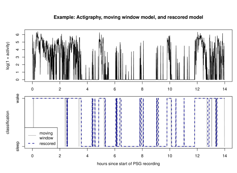
Figure 1: Example application of Webster’s rescoring rules – The top panel shows an example of activity over the course of the night, taken from the MESA dataset (see Section 4). A simple moving window classifier was applied to this activity trajectory, producing the sequence of sleep/wake classifications shown in the bottom panel, in gray. After applying the moving window classifier, Webster’s rescoring rules were applied, producing the blue, dashed line overlaid in the bottom panel. This rescoring procedure aims to correct for epochs erroneously classified as sleep.

By adjusting for long term patterns, these post hoc rules can make the accuracy of simple moving window models closer to that of recurrent neural network models (RNNs, Palotti et al.,, 2019). This improvement is intuitive, as RNNs often aim to find an optimal representation of long term patterns, after applying an initial moving window (i.e., convolutional) step. An advantage of Webster’s rules is that their interpretability helps users to understand when rescoring might not be appropriate, while black-box RNN rules can produce failures that are more difficult to identify.

Several disadvantages of Webster’s rules remain though. First, these rules do not produce continuous predicted class probabilities, only binary classifications. More importantly, these rules appear to have been derived heuristically through trial and error, rather than from being framed as a formal optimization problem. Some authors have presented alternative formulations of rescoring rules, but these appear to be heuristic as well (Qian et al.,, 2015; Kripke et al.,, 2010). Indeed, because of the somewhat complex structure of Webster’s rules, it is not immediately obvious how the constants $a,b,c$ and $d$ should be formally optimized, or how they should be recalibrated for new populations (Lüdtke et al.,, 2021; see also Heglum et al.,, 2021). These challenges deepen if we consider joint optimization of the moving window algorithm and the rescoring steps, rather than sequential optimization. Perhaps for these reasons, several modern papers on sleep-wake classification apply Webster’s rules as purely “off-the-shelf,” with no calibration (Tilmanne et al.,, 2009; Palotti et al.,, 2019; Liu et al.,, 2020).

These questions are the inspiration for our work. Namely, we demonstrate how rescoring rules can be optimized and/or calibrated by rephrasing these rules in terms of epoch-level features, such as the length of the most recent bout in a given state. Section 2 introduces these features, Section 3 discusses optimization methods, and Section 4 studies the performance of our approach in the Multi-Ethnic Study of Atherosclerosis (MESA) sleep study dataset (Chen et al.,, 2015; Zhang et al.,, 2018). We find that optimizing rules improves the performance of moving window models, although the difference is less pronounced for models with larger windows. We close with a discussion. In particular, we note that, while our proposed methods are motivated by sleep studies, they can also be applied to general, multi-state classification problems.

2 Rewriting rescoring rules with epoch-level features

In this section, as a first step towards choosing optimal parameters for rescoring rules (e.g., parameters $a,b,c$ and $d$ in Section 1), we will define a set of epoch-level, recursive features. We will then illustrate how Webster’s rescoring rules can be reexpressed in terms of those features.

Let $\mathbf{X}=(X_{1},\dots,X_{T})$, where $X_{t}$ is a sleep study participant’s activity summary at time $t$ during the night. Here, $t$ ranges from $1$ to $T$, with each value denoting one epoch. For simplicity of presentation, we omit an index for participants in a dataset, and instead focus on sleep/wake transitions for a single participant on a single night. Let $\mathbf{Y}=(Y_{1},\dots Y_{T})$, where $Y_{t}=1$ indicates wake at time $t$ and $Y_{t}=0$ indicates sleep at time $t$. For a given moving window algorithm applied to activity, let $\hat{\pi}=(\hat{\pi}_{1},\dots,\hat{\pi}_{T})$, where $\hat{\pi}_{t}$ is the estimate of $P(Y_{t}=1)$ produced by that algorithm. Let $\mathbf{W}=(W_{1},\dots W_{T})$, where $W_{t}\in\{0,1\}$ is a thresholded version of $\hat{\pi}_{t}$ and $W_{t}=1$ indicates a prediction of wake.

In order to capture long-term patterns in sleep, we define the several features for each epoch, indexed by $t$. These features have two general forms: (1) the time lag between $t$ and the most recent [or closest upcoming] bout of time spent in a given state, and (2) the length of the most recent [or closest upcoming] bout of time spent in a given state. More explicitly, we define these features as follows.

1. $\text{last}_{\text{lag}}^{\text{wake}}(\mathbf{Y},t)$: the time between $t$ and the most recent epoch $t^{\prime}\leq t$ for which $Y_{t^{\prime}}=1$.

2. $\text{last}_{\text{lag}}^{\text{sleep}}(\mathbf{Y},t)$: the time between $t$ and the most recent epoch $t^{\prime}\leq t$ for which $Y_{t^{\prime}}=0$.

3. $\text{last}_{\text{len}}^{\text{wake}}(\mathbf{Y},t)$: if $Y_{t}=0$, this feature returns the length of the most recent wake bout. If $Y_{t}=1$, it returns the cumulative length of the current wake bout.

4. $\text{last}_{\text{len}}^{\text{sleep}}(\mathbf{Y},t)$: if $Y_{t}=1$, this feature returns the length of the most recent sleep bout. If $Y_{t}=0$, it returns the cumulative length of the current sleep bout.

5. $\text{next}_{\text{lag}}^{\text{wake}}(\mathbf{Y},t)$: the time between $t$ and the closest upcoming epoch $t^{\prime}\geq t$ for which $Y_{t^{\prime}}=1$.

6. $\text{next}_{\text{lag}}^{\text{sleep}}(\mathbf{Y},t)$: the time between $t$ and the closest upcoming epoch $t^{\prime}\geq t$ for which $Y_{t^{\prime}}=0$.

7. $\text{next}_{\text{len}}^{\text{wake}}(\mathbf{Y},t)$: if $Y_{t}=0$, this feature returns the length of the closest upcoming wake bout. If $Y_{t}=1$, it returns the remaining length of the current wake bout.

8. $\text{next}_{\text{len}}^{\text{sleep}}(\mathbf{Y},t)$: if $Y_{t}=1$, this feature returns the length of the closest upcoming t sleep bout. If $Y_{t}=0$, it returns the remaining length of the current sleep bout.

Figure 2 illustrates how each of the above features transform their input, $\mathbf{Y}$. We refer to the first four features collectively as $l(\mathbf{Y},t)$, and refer to the last four features as $n(\mathbf{Y},t)$. The second set of features, $n(\mathbf{Y},t)$, can also be attained by reversing the time index of $l(\mathbf{Y},t)$. That is, if $\mathbf{Y}_{[T:1]}=(Y_{T},Y_{T-1},\dots Y_{2},Y_{1})$ is a time-reversed version of $\mathbf{Y}$, such that $(\mathbf{Y}_{[T:1]})_{t}=Y_{T-t+1}$, then $n(\mathbf{Y},t)=l(\mathbf{Y}_{[T:1]},T-t+1)$.

Additionally, given $l(\mathbf{Y},t)$ and $n(\text{{Y}},t)$, we can compute summaries of the sleep patterns surrounding any given epoch. In particular, we consider the following aggregate features.

1. $\text{current.total}_{\text{len}}^{\text{sleep}}(\mathbf{W},t)$: the length of the current sleep bout, equal to $\text{last}_{\text{lag}}^{\text{wake}}(\mathbf{W},t)+\text{next}_{\text{lag}}^{\text{wake}}(\mathbf{W},t).$

2. $\text{\text{current.total}}_{\text{len}}^{\text{wake}}(\mathbf{W},t):$ the length of the current wake bout, equal to $\text{last}_{\text{lag}}^{\text{sleep}}(\mathbf{W},t)+\text{next}_{\text{lag}}^{\text{sleep}}(\mathbf{W},t)$.

3. $\text{min.bordering}_{\text{len}}^{\text{sleep}}(\mathbf{W},t)$: the length of the smallest bordering sleep bout, equal to $\min\left(\text{\text{last}}_{\text{len}}^{\text{sleep}}(\mathbf{W},t),\text{\text{next}}_{\text{len}}^{\text{sleep}}(\mathbf{W},t)\right)$.

4. $\text{min.bordering}_{\text{len}}^{\text{wake}}(\mathbf{W},t)$: the length of the smallest bordering wake bout, equal to $\min\left(\text{\text{last}}_{\text{len}}^{\text{wake}}(\mathbf{W},t),\text{\text{next}}_{\text{len}}^{\text{wake}}(\mathbf{W},t)\right)$.

We refer to the above four features as $c(\mathbf{Y},t)$.

An important property of these 12 features is that they can all be defined recursively (shown in Appendix A). Given $l(\mathbf{Y},t-1)$, the features $l(\mathbf{Y},t)$ depend only on $Y_{t}$. Similarly, given $n(\mathbf{Y},t+1)$, the features $n(\mathbf{Y},t)$ depend only on $Y_{t}$. Further, given $l(\mathbf{Y},t-1)$ and $n(\mathbf{Y},t+1)$ the features $l(\mathbf{Y},t)$ and $n(\mathbf{Y},t)$ are both linear in $Y_{t}$ (see Appendix A). From here, $c(\mathbf{Y},t)$ is determined immediately from $(l(\mathbf{Y},t),n(\mathbf{Y},t)$). This recursive structure will prove useful in the next section, and is illustrated in Figure 4.

In practice, none of the above features are known for unlabeled data, but they can be approximated by plugging in $\mathbf{W}$ for $\mathbf{Y}$ to yield the vector of rescoring features $r(\mathbf{W},t):=(W_{t},l(\mathbf{W},t),n(\mathbf{W},t),c(\mathbf{W},t))$. Since $l(\mathbf{W},1)$ and $n(\mathbf{W},T)$ depend on information outside of the time period in which participants are observed, we require user-supplied tuning parameters $b_{1},b_{T}\in\mathbb{R}_{\geq 0}^{4}$, and set these border values to be $l(\mathbf{W},1)=b_{1}$ and $n(\mathbf{W},T)=b_{T}$.

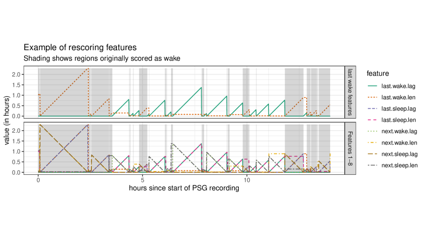
Figure 2: Example of rescoring features – Here we show the rescoring features, computed as a function of the classification sequence shown in the bottom panel of Figure 3 ($W_{t}$, gray line). The original classification from the moving window model $(W_{t}$) is shown here via shading, with gray corresponding to regions classified as wake. The first panel shows two rescoring features, $\text{last}_{\text{lag}}^{\text{wake}}(\mathbf{W},t)$ and $\text{last}_{\text{len}}^{\text{wake}}(\mathbf{W},t)$. These two functions represent the core operations of our proposed procedure – all other values in $(l(\mathbf{W},t),n(\mathbf{W},t))$ can be found reversing the time index (x-axis) and/or by flipping the original score (shading). The second panel shows the 8 features in $(l(\mathbf{W},t),n(\mathbf{W},t))$ together.

Finally, with these features in mind, we can see that the two general forms of Webster’s rescoring rules can be rewritten as follows.

Rule  1:

if $\text{last}_{\text{len}}^{\text{wake}}(\mathbf{W},t)\geq a$ and $\text{last}_{\text{lag}}^{\text{wake}}(\mathbf{W},t)\leq b$, then rescore the $t^{th}$ epoch as wake.

Rule  2:

if $\text{current.total}_{\text{len}}^{\text{sleep}}(\mathbf{W},t)\leq c$ and $\text{min.bordering}_{\text{len}}^{\text{wake}}(\mathbf{W},t)\geq d$, then rescore the $t^{th}$ epoch as wake.

Any epoch that does not meet either of these rules for any of the allowed values of $a,b,c$ and $d$ retains its original score ($W_{t}$). In other words, Webster’s rules form a decision tree with $r(\mathbf{W},t)$ as input (see Figure 3).

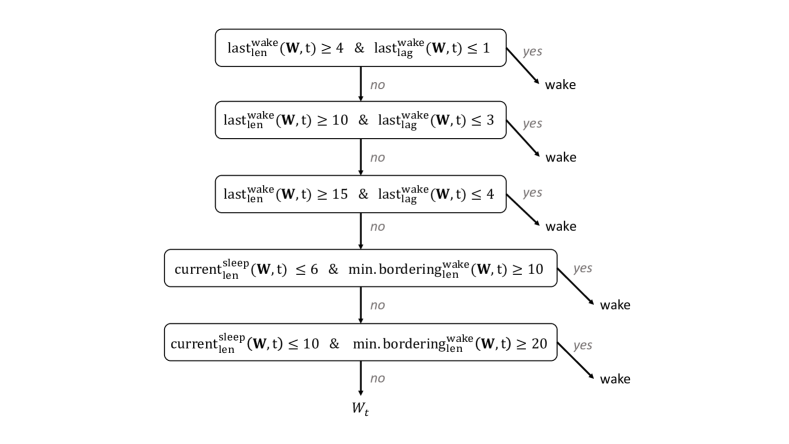
Figure 3: Webster’s rescoring rules rewritten in terms of the features from Section 2. This tree returns the rescored prediction of sleep/wake status at epoch $t$.

3 Optimizing rescoring rules

As Webster’s rescoring rules are a heuristically chosen function of $r(\mathbf{W},t)$, a natural next step is to search for an optimal function of $r(\mathbf{W},t)$. This is especially straightforward if we treat the original scores $\mathbf{W}$ as fixed, in which case we can apply any off-the-shelf training algorithm to find a classifier of $Y_{t}$ based on $r(\mathbf{W},t)$. One caveat is that, since $c(\mathbf{W},t)$ includes linear combinations of $l(\mathbf{W},t)$ and $n(\mathbf{W},t)$, it cannot be included alongside $l(\mathbf{W},t)$ and $n(\mathbf{W},t)$ in models that require linearly independent covariates (e.g., logistic regression models), at least not without first applying a log or other nonlinear transformation.

We can also choose to include a continuous version of $r\left(\mathbf{W},t\right)$ in our classifier. One straightforward implementation is to replace $W_{t}$ with the unthresholded probabilities $\hat{\pi}$, forming $r(\hat{\pi},t)=\left(\hat{\pi},l(\hat{\pi},t),n(\hat{\pi},t),c(\hat{\pi},t)\right)$. This implementation can be motivated by the working model assumption that, given $\mathbf{X}$, the wake indicators $(Y_{1},\dots,Y_{T})$ are independently distributed Bernoulli variables with $P(Y_{t}=1|\mathbf{X})=\hat{\pi}_{t}$. Since each element of $\left(l(\hat{\pi},t),n(\hat{\pi},t)\right)$ is linear in $Y_{t}$ given its neighbors, it follows from this working model that $E\left[l(\mathbf{Y},t)|\mathbf{X}\right]=l(\hat{\pi},t)$ and $E\left[n(\mathbf{Y},t)|\mathbf{X}\right]=n(\hat{\pi},t)$ (see Appendix C).

From here, we can jointly optimize the continuous features $\hat{\pi}_{t}$ and the model fit to the features $r\left(\hat{\pi}_{t},t\right)$ using gradient-based optimization software, such as PyTorch or Tensorflow (Abadi et al.,, 2015; Paszke et al.,, 2017). For example, consider the multi-layer model

$$P(Y_{t}=1|\mathbf{X})=\text{logit}^{-1}\left[\alpha_{1}+\left(\text{logit}(\hat{\pi}_{t}),\log\left\{1+\left(l\left(\hat{\pi},t\right),n\left(\hat{\pi},t\right),c\left(\hat{\pi},t\right)\right)\right\}\right)^{\top}\beta_{1}\right],$$ (1)

where

$$\hat{\pi}_{t}=\text{logit}^{-1}\left(\alpha_{0}+\left[\begin{array}[]{cccc}X_{t+a}&X_{t+a+1}&\dots&X_{t+b}\end{array}\right]\beta_{0}\right).$$ (2)

Above, $(\alpha_{0},\alpha_{1},\beta_{0},\beta_{1})$ are model parameters, and $(a,b)$ are tuning parameters determining the size of a moving window, chosen to satisfy $a\leq 0\leq b$. Under this model, the likelihood of $Y_{t}$ given $\mathbf{X}$ is a differentiable (almost everywhere) function of $(\alpha_{0},\alpha_{1},\beta_{0},\beta_{1})$, and so maximum likelihood estimates can be attained using gradient-based methods. While the requirement that we use the continuous quantity $\hat{\pi}$ (rather than $\mathbf{W}$) may appear restrictive, we note that $\hat{\pi}$ can be made arbitrarily close to a binary variable by increasing the scale of $(\alpha_{0},\beta_{0})$. For our implementation, we train the model in Eqs (1)-(2) using the r Keras package (Chollet et al.,, 2017), with a customized recurrent layer to represent $r\left(\hat{\pi},t\right)$. The structure of the resulting network is shown in Figure 4.

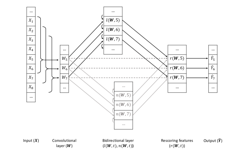
Figure 4: Rescoring pipeline – Here we show the general structure of Webster’s rescoring rules, where the moving window model output $(W_{t})$ is treated as fixed. For the purposes of this illustration, the input to the moving window model is $(X_{t-4},X_{t-3},X_{t-2},X_{t-1},X_{t},X_{t+1})$. Each box refers to an epoch-level variable, or feature vector. Arrows indicate the inputs for each feature. Webster’s rescoring rules can be interpreted as one way to transform from the penultimate layer $r(\hat{\pi}_{t},t)$ to the prediction $\hat{Y}_{t}$. The sequential optimization approach in Section 3 can be attained by optimizing this transformation. The joint optimization approach in Section 3 can be attained by replacing each thresholded $W_{t}$ with a continuous probability, and jointly optimizing both the convolutional layer and the transformation from rescoring features to final predictions, while fixing the intervening layers based on intuitive patterns suggested by Webster et al., (1982).

4 Performance comparison with MESA dataset

In this section, we compare the performance of standard MWAs, MWAs with off-the-shelf Webster’s rescoring rules, and MWAs with calibrated rescoring rules. In calibrating these rules, we apply both sequential and joint optimization approaches. We evaluate these methods using the commercial use dataset from the Multi-Ethnic Study of Atherosclerosis (MESA), a longitudinal study of cardiovascular disease (Chen et al.,, 2015; Zhang et al.,, 2018; see also Palotti et al.,, 2019). One night of concurrent actigraphy and scored polysomnography (PSG) was recorded for many of the participants in this study. After filtering to participants with at least 5 hours of contiguously measured actigraphy and PSG, our dataset included 1685 individuals.

As a baseline prediction model, we fit logistic regressions to predict sleep state $Y_{t}$ using the variables $(X_{t+a},X_{t+a+1},X_{t+a+2},\dots X_{t+b})$ as input (referred to as “GLM-window”). We considered three window sizes, setting $[a,b]$ equal to $[-5,2]$, $[-10,5]$ and $[-30,20]$. For each model, we also applied “off-the-shelf” Webster’s rescoring rules (referred to as “Webster”).

For sequentially optimized rescoring rules, we applied the transformations in Section 2 to the output of the three logistic regression models above. For each window size, we fit a second, post hoc logistic regression to predict sleep state $Y_{t}$ using $\text{logit}(\hat{\pi})$, $\log\{1+l(\hat{\pi},t)\}$, $\log\{1+n(\hat{\pi},t)\}$, and $\log\{1+c(\hat{\pi},t)\}$ as input (referred to as “GLM-continuous”), where $\hat{\pi}$ is the vector of predicted wake probabilities produced by the “GLM-window” method. We also fit logistic regressions taking ($\hat{\pi},l(\mathbf{W},t),n(\mathbf{W},t),c(\mathbf{W},t)$) as input, using 0.5 as the threshold for $\mathbf{W}$ (“GLM-binary”).

To jointly optimize the rescoring rules, we used the r Keras implementation described in Section 3 (“rescore-NN”). As above, we considered three window sizes: $[-5,2]$, $[-10,5]$, and $[-30,20]$. We initialized each model using the coefficients from the “GLM-window” and “GLM-continuous” methods. After initialization, we trained each model with a batch size of 100, and 20 epochs.

As a benchmark representing more complex prediction models, we compared against neural networks with three layers: (1) a 1-dimensional convolutional layer taking activity as input; (2) a bi-directional, long short-term memory (LSTM) layer taking the output of Layer 1 as input; and (3) a linear layer taking the output of both Layer 1 and Layer 2 as input (analogous to Figure 4). We implemented this structure again using the r Keras package (Chollet et al.,, 2017), and considered two configurations, referred to as “LSTM-1-6” and “LSTM-10-30.” The first configuration, “LSTM-1-6,” was meant to mimic the structure and initialization procedure of “rescore-NN,” with a single convolutional filter and 6 hidden variables in each direction of the LSTM layer (12 total). We initialized Layer 1’s weights based on the “GLM-window” model, and initialized Layer 3’s weights to be 1 for the Layer 1 output, and zero elsewhere. Thus, at initialization, “LSTM-1-6” produces predictions identical to “GLM-window.” The second configuration, “LSTM-10-30,” allowed for a more complex structure, with 10 filters in the convolutional layer and 30 hidden variables in each direction of the LSTM layer. As above, both configurations were fit using windows of $[-5,2]$, $[-10,5]$ and $[-30,20]$ for the convolutional layer. The batch size and number of epochs were again set to 100 and 20 respectively.

We evaluated performance using 5-fold cross-validation, computing Receiver Operating Characteristic (ROC) curves for each prediction model. To attain ROC curves for Webster’s rules, varied the threshold used to define $\mathbf{W}$.

Figure 5 shows ROC curves from our analysis, and Table 1 shows the area under each curve (AUC). Webster’s rules gave a small performance improvement over our simplest model, “GLM-window.” Sequentially optimizing the rescoring rules (“GLM-continuous” and “GLM-binary”) added another small improvement over Webster’s rules. Jointly optimizing the moving window weights and the rescoring rules (“rescore-NN”) had a negligible effect on performance, relative to “GLM-continuous.” Our optimized rescoring methods outperformed the LSTM models implementations described above. That said, this result does not preclude the possibility of other neural network architectures generating better performance from LSTM layers. The differences between the above methods were also diminished when longer windows were used.

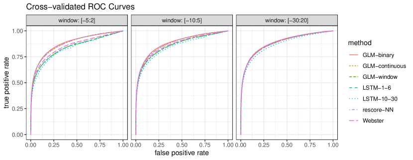
Figure 5: Receiver Operating Characteristic ROC curves for each model.

	Window
Method	[-5:2]	[-10:5]	[-30:20]
GLM-binary	0.879	0.882	0.888
GLM-continuous	0.877	0.880	0.886
GLM-window	0.836	0.860	0.882
LSTM-1-6	0.837	0.860	0.882
LSTM-10-30	0.827	0.846	0.868
rescore-NN	0.877	0.880	0.886
Webster	0.850	0.867	0.882

Table 1: Areas under the ROC curves in Figure 5. Variations of our proposed method are bolded.

As an additional illustration of what optimized versions of rescoring rules could resemble, Figure 6 shows a version of the tree in Figure 3 trained on all 1685 participants. The input to the tree is a vector of rescoring features $r(\mathbf{W},t)$, where $\mathbf{W}$ is the binarized output of a moving window, logistic regression model, with a window of $[-10,5]$. Here, the rescoring operation is simplified to a single rule: any bout of predicted sleep lasting less than 14 minutes is rescored as wake.

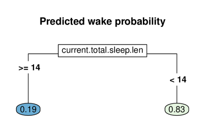
Figure 6: A version of Webster’s rescoring rules, calibrated to the MESA dataset. Current, total sleep length is measured in minutes.

5 Discussion

We have demonstrated how rescoring rules can be optimized for any population of interest by reframing the rules in terms of epoch-level features. In tests with the MESA dataset, we find our procedure to produce accuracy comparable to certain configurations of LSTM networks. That said, the improvement achieved by optimizing rescoring rules is less noticeable when the initial moving window model has a wide window. This limitation is intuitive, as some of the long-term information otherwise gained from the rescoring rules is already attained from the larger window. The implication of our applied analysis is that larger windows, and optimization steps, should both be explored whenever Webster’s rescoring rules are used. This includes performance tests where rescoring rules are used as a benchmark representing simple, interpretable methods.

Our work opens up several avenues for future sleep-wake classification methods. One simple extension would be to include other wearable device measurements, such as heart rate, in the moving window model. Another extension would be to explore other types of machine learning models fit to the epoch-level features in Section 2. Digging more deeply, while we have held the formulas of our epoch-level features ($l(\mathbf{W},t),n(\mathbf{W},t)$) fixed (see Appendix A), it could be fruitful to explore versions of these features with trainable parameters. Rescoring features could also be implemented in other neural network architectures. For example, these transformations could be separately applied to the output of several convolutional filters, or additional layers could be stacked between the rescoring features $r(\mathbf{W},t)$ and the final predictions (See Figure 4).

An important caveat is that any joint optimization approach complicates the interpretation of the rescoring rules, as their input is no longer an estimated wake probability. This limitation is also true of our Keras implementation (“rescore-NN”), but becomes especially problematic in more complex network architectures. Even so, rescoring features may still be helpful in regularizing prediction pipelines.

Our rescoring approach also immediately generalizes to multi-state classification problems, such as general activity classification (e.g., sitting, walking, or stair climbing) or sleep stage classification. For each state $k$, we can define epoch-level features such as “the time between now and the most recent (or closest upcoming) bout of time in state $k$,” using the same techniques as above (see Appendix A). In this way, rescoring features could provide a promising means of incorporating long-term information into general temporal modeling problems.

Appendix A Recursive definitions for $n(\mathbf{Y},t)$ and $l(\mathbf{Y},t)$

Let $\epsilon$ be the length of an epoch. For $t>1$, let

$$\text{last}_{\text{lag}}^{\text{wake}}(\mathbf{Y},t):=\left(1-Y_{t}\right)\left\{\text{last}_{\text{lag}}^{\text{wake}}(\mathbf{Y},t-1)+\epsilon\right\},$$ (3)

$$\text{last}_{\text{lag}}^{\text{sleep}}(\mathbf{Y},t):=Y_{t}\left\{\text{last}_{\text{lag}}^{\text{sleep}}(\mathbf{Y},t-1)+\epsilon\right\},$$

$$\text{last}_{\text{len}}^{\text{wake}}(\mathbf{Y},t) :=(1-Y_{t})\,\text{last}_{\text{len}}^{\text{wake}}(\mathbf{Y},t-1)+Y_{t}\,\text{last}_{\text{lag}}^{\text{sleep}}(\mathbf{Y},t)$$

$$=(1-Y_{t})\,\text{last}_{\text{len}}^{\text{wake}}(\mathbf{Y},t-1)+Y_{t}^{2}\,\left\{\text{last}_{\text{lag}}^{\text{sleep}}(\mathbf{Y},t-1)+\epsilon\right\}$$

$$=(1-Y_{t})\,\text{last}_{\text{len}}^{\text{wake}}(\mathbf{Y},t-1)+Y_{t}\,\left\{\text{last}_{\text{lag}}^{\text{sleep}}(\mathbf{Y},t-1)+\epsilon\right\},$$

and

$$\text{last}_{\text{len}}^{\text{sleep}}(\mathbf{Y},t) :=Y_{t}\,\text{last}_{\text{len}}^{\text{sleep}}(\mathbf{Y},t-1)+(1-Y_{t})\,\left\{\text{last}_{\text{lag}}^{\text{wake}}(\mathbf{Y},t-1)+\epsilon\right\}.$$ (4)

Following the same logic, for $t<T$, let

$$\text{next}_{\text{lag}}^{\text{wake}}(\mathbf{Y},t):=(1-Y_{t})\left\{\text{next}_{\text{lag}}^{\text{wake}}(\mathbf{Y},t+1)+\epsilon\right\},$$

$$\text{next}_{\text{lag}}^{\text{sleep}}(\mathbf{Y},t):=Y_{t}\left\{\text{next}_{\text{lag}}^{\text{sleep}}(\mathbf{Y},t+1)+\epsilon\right\},$$

$$\text{next}_{\text{len}}^{\text{wake}}(\mathbf{Y},t):=(1-Y_{t})\,\text{\text{next}}_{\text{len}}^{\text{wake}}(\mathbf{Y},t+1)+Y_{t}\,\left\{\text{\text{next}}_{\text{lag}}^{\text{sleep}}(\mathbf{Y},t+1)+\epsilon\right\},$$

and

$$\text{next}_{\text{len}}^{\text{sleep}}(\mathbf{Y},t):=Y_{t}\,\text{\text{next}}_{\text{len}}^{\text{sleep}}(\mathbf{Y},t+1)+(1-Y_{t})\,\left\{\text{\text{next}}_{\text{lag}}^{\text{wake}}(\mathbf{Y},t+1)+\epsilon\right\}.$$

It is fairly straightforward to generalize these features to the multi-state setting. For each state $k$, we simply replace $Y_{t}$ with the indicator $1(Y_{t}=k)$. The four “wake” features above then describe bouts of time in state $k$, and the four “sleep” features describe bouts of time not spent in state $k$. In this way, the multi-state setting generates approximately twice as many features per state as the binary setting, since we additionally keep track of bouts of time spent in any state but state $k$. These extra states are required for our proposed computation of bout length (e.g., Eq 4).

Alternatively, these extra states can be removed if we instead use a min operation when computing bout length. That is, we can set

$$\text{last}_{\text{len}}^{k}(\mathbf{Y},t):=\left\{1-1(Y_{t}=k)\right\}\,\text{last}_{\text{len}}^{k}(\mathbf{Y},t-1)+1(Y_{t}=k)\,\min_{k^{\prime}\neq k}\left\{\text{last}_{\text{lag}}^{k^{\prime}}(\mathbf{Y},t-1)+\epsilon\right\}$$

to be the length of the most recent bout in state $k$, and set

$$\text{last}_{\text{lag}}^{k}(\mathbf{Y},t):=\left\{1-1(Y_{t}=k)\right\}\left\{\text{last}_{\text{lag}}^{k}(\mathbf{Y},t-1)+\epsilon\right\}$$

to be the time since that bout.

Appendix B Vectorized versions of rescoring features

The four formulas in Eqs (3)-(4) can also be vectorized as follows.

$$\left[\begin{array}[]{c}\text{last}_{\text{lag}}^{\text{wake}}(\mathbf{Y},t)\\ \text{last}_{\text{lag}}^{\text{sleep}}(\mathbf{Y},t)\\ \text{last}_{\text{len}}^{\text{wake}}(\mathbf{Y},t)\\ \text{last}_{\text{len}}^{\text{sleep}}(\mathbf{Y},t)\end{array}\right] =\left[\begin{array}[]{c}\epsilon\\ 0\\ 0\\ \epsilon\end{array}\right]+\left[\begin{array}[]{c}-\epsilon\\ \epsilon\\ \epsilon\\ -\epsilon\end{array}\right]Y_{t}$$ (17)

$$\hskip 10.00002pt+\left(\left[\begin{array}[]{cccc}1&0&0&0\\ 0&0&0&0\\ 0&0&1&0\\ 1&0&0&0\end{array}\right]+\left[\begin{array}[]{cccc}-1&0&0&0\\ 0&1&0&0\\ 0&1&-1&0\\ -1&0&0&1\end{array}\right]Y_{t}\right)\left[\begin{array}[]{c}\text{last}_{\text{lag}}^{\text{wake}}(\mathbf{Y},t-1)\\ \text{last}_{\text{lag}}^{\text{sleep}}(\mathbf{Y},t-1)\\ \text{last}_{\text{len}}^{\text{wake}}(\mathbf{Y},t-1)\\ \text{last}_{\text{len}}^{\text{sleep}}(\mathbf{Y},t-1)\end{array}\right].$$ (30)

Or, in more compact notation,

$$l(\mathbf{Y},t)=\mathbf{v}_{0}+Y_{t}\mathbf{v}_{1}+(\mathbf{M}_{0}+Y_{t}\mathbf{M}_{1})l(\mathbf{Y},t-1),$$

where $\mathbf{v}_{0}$ and $\mathbf{v}_{1}$ are the two vectors on the right-hand side of Line (17), and $\mathbf{M}_{0}$ and $\mathbf{M}_{1}$ are the two matrices in Line (30). Similarly,

$$n(\mathbf{Y},t)=\mathbf{v}_{0}+Y_{t}\mathbf{v}_{1}+(\mathbf{M}_{0}+Y_{t}\mathbf{M}_{1})n(\mathbf{Y},t+1).$$

Appendix C Conditional expectation of $l(\mathbf{Y},t)$ and $n(\mathbf{Y},t)$

In this section we show the claim from Section 3 that if $(Y_{1},\dots,Y_{T})$ are independently distributed Bernoulli variables, given $\mathbf{X}$, with $P(Y_{t}=1|\mathbf{X})=\hat{\pi}_{t}$, then $E\left[l(\mathbf{Y},t)|\mathbf{X}\right]=l(\hat{\pi},t)$ and $E\left[n(\mathbf{Y},t)|\mathbf{X}\right]=n(\hat{\pi},t)$.

For $l(\mathbf{Y},t)$ we show this by induction. The base case holds by definition, since $E\left[l(\mathbf{Y},1)|\mathbf{X}\right]=b_{1}=l(\hat{\pi},1)$. For the inductive step, note that $l(\mathbf{Y},t)$ depends only on $(Y_{1},\dots,Y_{t})$. If $E\left[l(\mathbf{Y},t-1)|\mathbf{X}\right]=l(\hat{\pi},t-1)$, then the vector representations in the previous section tell us that

$$E\left[l(\mathbf{Y},t)|\mathbf{X}\right]$$

$$=E\left[E\left\{l(\mathbf{Y},t)|Y_{1},\dots,Y_{t-1},\mathbf{X}\right\}\,|\,\mathbf{X}\right]$$

$$=E\left[E\left\{\mathbf{v}_{0}+Y_{t}\mathbf{v}_{1}+(\mathbf{M}_{0}+Y_{t}\mathbf{M}_{1})l(\mathbf{Y},t-1)\hskip 10.00002pt|\hskip 10.00002ptY_{1},\dots,Y_{t-1},\mathbf{X},l(\mathbf{Y},t-1)\right\}\,|\,\mathbf{X}\right]$$

$$=E\left[E\left\{\mathbf{v}_{0}+Y_{t}\mathbf{v}_{1}+(\mathbf{M}_{0}+Y_{t}\mathbf{M}_{1})l(\mathbf{Y},t-1)\hskip 10.00002pt|\hskip 10.00002pt\mathbf{X},l(\mathbf{Y},t-1)\right\}\,|\,\mathbf{X}\right]$$

$$=E\left[\mathbf{v}_{0}+E\left\{Y_{t}|l(\mathbf{Y},t-1),\mathbf{X}\right\}\mathbf{v}_{1}+(\mathbf{M}_{0}+E\left\{Y_{t}|l(\mathbf{Y},t-1),\mathbf{X}\right\}\mathbf{M}_{1})l(\mathbf{Y},t-1)\,|\,\mathbf{X}\right]$$

$$=E\left[\mathbf{v}_{0}+E\left\{Y_{t}|\mathbf{X}\right\}\mathbf{v}_{1}+(\mathbf{M}_{0}+E\left\{Y_{t}|\mathbf{X}\right\}\mathbf{M}_{1})l(\mathbf{Y},t-1)\,|\,\mathbf{X}\right]$$ (31)

$$=E\left[\mathbf{v}_{0}+\hat{\pi}_{t}\mathbf{v}_{1}+(\mathbf{M}_{0}+\hat{\pi}_{t}\mathbf{M}_{1})l(\mathbf{Y},t-1)\,|\,\mathbf{X}\right]$$

$$=\mathbf{v}_{0}+\hat{\pi}_{t}\mathbf{v}_{1}+(\mathbf{M}_{0}+\hat{\pi}_{t}\mathbf{M}_{1})E\left[l(\mathbf{Y},t-1)\,|\,\mathbf{X}\right]$$

$$=\mathbf{v}_{0}+\hat{\pi}_{t}\mathbf{v}_{1}+(\mathbf{M}_{0}+\hat{\pi}_{t}\mathbf{M}_{1})l(\hat{\pi},t-1)$$

$$=l(\hat{\pi},t).$$

Above, Line (31) comes from our assumption of conditional independence.

The same steps can be used to show that $E\left[n(\mathbf{Y},t)|\mathbf{X}\right]=n(\hat{\pi},t)$.

References

- Abadi et al., (2015) Abadi, M., Agarwal, A., Barham, P., Brevdo, E., Chen, Z., Citro, C., Corrado, G. S., Davis, A., Dean, J., Devin, M., Ghemawat, S., Goodfellow, I., Harp, A., Irving, G., Isard, M., Jia, Y., Jozefowicz, R., Kaiser, L., Kudlur, M., Levenberg, J., Mané, D., Monga, R., Moore, S., Murray, D., Olah, C., Schuster, M., Shlens, J., Steiner, B., Sutskever, I., Talwar, K., Tucker, P., Vanhoucke, V., Vasudevan, V., Viégas, F., Vinyals, O., Warden, P., Wattenberg, M., Wicke, M., Yu, Y., and Zheng, X. (2015). TensorFlow: Large-scale machine learning on heterogeneous systems. Software available from tensorflow.org.
- Benson et al., (2004) Benson, K., Friedman, L., Noda, A., Wicks, D., Wakabayashi, E., and Yesavage, J. (2004). The measurement of sleep by actigraphy: direct comparison of 2 commercially available actigraphs in a nonclinical population. Sleep, 27(5):986–989.
- Chen et al., (2015) Chen, X., Wang, R., Zee, P., Lutsey, P. L., Javaheri, S., Alcántara, C., Jackson, C. L., Williams, M. A., and Redline, S. (2015). Racial/Ethnic differences in sleep disturbances: The Multi-Ethnic study of atherosclerosis (MESA). Sleep, 38(6):877–888.
- Chollet et al., (2017) Chollet, F., Allaire, J., et al. (2017). R interface to keras. https://github.com/rstudio/keras.
- Cole et al., (1992) Cole, R. J., Kripke, D. F., Gruen, W., Mullaney, D. J., and Gillin, J. C. (1992). Automatic sleep/wake identification from wrist activity. Sleep, 15(5):461–469.
- Haghayegh et al., (2020) Haghayegh, S., Khoshnevis, S., Smolensky, M. H., and Diller, K. R. (2020). Application of deep learning to improve sleep scoring of wrist actigraphy. Sleep Med., 74:235–241.
- Haghayegh et al., (2019) Haghayegh, S., Khoshnevis, S., Smolensky, M. H., Diller, K. R., and Castriotta, R. J. (2019). Performance comparison of different interpretative algorithms utilized to derive sleep parameters from wrist actigraphy data. Chronobiol. Int., 36(12):1752–1760.
- Heglum et al., (2021) Heglum, H. S. A., Kallestad, H., Vethe, D., Langsrud, K., Engstrøm, M., et al. (2021). Distinguishing sleep from wake with a radar sensor a contact-free real-time sleep monitor. Sleep.
- Jean-Louis et al., (2000) Jean-Louis, G., Kripke, D. F., Ancoli-Israel, S., Klauber, M. R., and Sepulveda, R. S. (2000). Sleep duration, illumination, and activity patterns in a population sample: effects of gender and ethnicity. Biological psychiatry, 47(10):921–927.
- Kripke et al., (2010) Kripke, D. F., Hahn, E. K., Grizas, A. P., Wadiak, K. H., Loving, R. T., Poceta, J. S., Shadan, F. F., Cronin, J. W., and Kline, L. E. (2010). Wrist actigraphic scoring for sleep laboratory patients: algorithm development. Journal of sleep research, 19(4):612–619.
- Liu et al., (2020) Liu, J., Zhao, Y., Lai, B., Wang, H., and Tsui, K. L. (2020). Wearable device heart rate and activity data in an unsupervised approach to personalized sleep monitoring: Algorithm validation. JMIR Mhealth Uhealth, 8(8):e18370.
- Lüdtke et al., (2021) Lüdtke, S., Hermann, W., Kirste, T., Beneš, H., and Teipel, S. (2021). An algorithm for actigraphy-based sleep/wake scoring: Comparison with polysomnography. Clin. Neurophysiol., 132(1):137–145.
- Oakley, (1997) Oakley, N. R. (1997). Validation with polysomnography of the sleepwatch sleep/wake scoring algorithm used by the actiwatch activity monitoring system. Bend: Mini Mitter, Cambridge Neurotechnology.
- Palotti et al., (2019) Palotti, J., Mall, R., Aupetit, M., Rueschman, M., Singh, M., Sathyanarayana, A., Taheri, S., and Fernandez-Luque, L. (2019). Benchmark on a large cohort for sleep-wake classification with machine learning techniques. NPJ Digit Med, 2:50.
- Paszke et al., (2017) Paszke, A., Gross, S., Chintala, S., Chanan, G., Yang, E., DeVito, Z., Lin, Z., Desmaison, A., Antiga, L., and Lerer, A. (2017). Automatic differentiation in pytorch.
- Qian et al., (2015) Qian, X., Hao, H., Chen, Y., and Li, L. (2015). Wake/sleep identification based on body movement for parkinson’s disease patients. Journal of Medical and Biological Engineering, 35(4):517–527.
- Sadeh et al., (1994) Sadeh, A., Sharkey, K. M., and Carskadon, M. A. (1994). Activity-based sleep-wake identification: an empirical test of methodological issues. Sleep, 17(3):201–207.
- Sazonov et al., (2004) Sazonov, E., Sazonova, N., Schuckers, S., Neuman, M., and CHIME Study Group (2004). Activity-based sleep–wake identification in infants. Physiol. Meas., 25(5):1291.
- Tilmanne et al., (2009) Tilmanne, J., Urbain, J., Kothare, M. V., Wouwer, A. V., and Kothare, S. V. (2009). Algorithms for sleep–wake identification using actigraphy: a comparative study and new results. Journal of sleep research, 18(1):85–98.
- Webster et al., (1982) Webster, J. B., Kripke, D. F., Messin, S., Mullaney, D. J., and Wyborney, G. (1982). An activity-based sleep monitor system for ambulatory use. Sleep, 5(4):389–399.
- Zhang et al., (2018) Zhang, G.-Q., Cui, L., Mueller, R., Tao, S., Kim, M., Rueschman, M., Mariani, S., Mobley, D., and Redline, S. (2018). The national sleep research resource: towards a sleep data commons. J. Am. Med. Inform. Assoc., 25(10):1351–1358.