To Code, or Not to Code, at the Racetrack: Kelly Betting and Single-Letter Codes

Abstract

For a gambler with side information, Kelly betting gives the optimal log growth rate of the gambler’s fortune, which is closely related to the mutual information between the correct winner and the noisy side information. We show conditions under which optimal Kelly betting can be implemented using single-letter codes. We show that single-letter coding is optimal for a wide variety of systems; for example, all systems with diagonal reward matrices admit optimal single-letter codes. We also show that important classes of systems do not admit optimal single-letter codes for Kelly betting, such as when the side information is passed through a Z channel. Our results are important to situations where the computational complexity of the gambler is constrained, and may lead to new insights into the fitness value of information for biological systems.

I Introduction

Consider a series of races between two horses, where each race is independent, and each horse has a prior probability $p=\frac{1}{2}$ of winning a race. Bets can be placed on the the races, paying fair odds: double the bet for a win, and zero for a loss. Suppose a gambler has access to side information, and can guess the winner of each race with probability $q$, where $\frac{1}{2}<q<1$; further suppose the gambler wants to maximize the logarithm of their rate of return over time. Then with the optimal strategy, the log return is equal to the Shannon capacity $C$ of the “channel” between the race winner $W$ and the gambler’s guess using the side information $Y$ [1].

Instead, suppose the side information is generated by a genie, who knows in advance the outcome of every race, and sends this information to the gambler, one bit per race, over a noisy (binary symmetric) channel with error probability $q$. If the genie and the gambler agree to use an optimal error-correcting code, to give the gambler perfect knowledge of as many winners as possible, then the gambler can learn no more than a fraction $C$ of the winners. With fair odds, the log return with perfect knowledge is $\log 2=1$, while the best log return with only the prior information is $\log 1=0$, so the average log return is merely $C$.

For this simple example, the gambler would do just as well if the genie and gambler agree not to use any error-correcting code: if the winners are sent through the binary symmetric channel without coding, the gambler can guess the winner with probability $q$, and can use Kelly betting to obtain a log return of $C$. In fact, for this system it can be shown that no coding approach gives a log return higher than $C$. For more general systems, under some conditions, single-letter (i.e., memoryless) codes can achieve the minimum average distortion at a given rate [2]. The main contribution of this paper is to show that optimal Kelly betting satisfies these conditions under a wide range of circumstances.

In his original paper [1], Kelly found that when no side information is available, the optimal strategy is for the gambler to split her wealth into bets according to the probability of each horse winning, a strategy called proportional betting. When side information is available, the optimal strategy is to instead bet according to the conditional probability of a horse winning given the side information. This work has been extended for applications in fields such as portfolio theory [3, 4, 5, 6] and evolutionary biology [7, 8, 9, 10, 11, 12, 13]. For growing populations of organisms sensing and responding to environmental cues, the mutual information can be interpreted as the fitness value of the information provided by the environmental cues.

In biological systems, the betting strategy is implemented through the mix of phenotypes in the population, and decisions taken at the level of the individual cell to switch among phenotypes. There are numerous examples of phenotype switching in biological populations [14], such as the plasticity of cancer cells [15], persistence of bacteria in the presence of antibiotics [16, 17, 18], alteration of pigment expression in cyanobacteria [19], and development of lungs by amphibious fish [20]. The abundance of evidence for phenotype switching across the taxa suggests that an information theoretic analysis of population growth is highly relevant to understanding evolution. However, to our knowledge the conditions under which single-letter Kelly-type strategies are optimal have not been previously investigated, although applications of these conditions to biological systems have been mentioned [2, 10].

In this article, we formulate Kelly-like gambling problems in the context of rate distortion theory. Our distortion function is defined in terms of wealth growth rate loss due to noise in the side information channel, while the cost function is defined as a function of the growth rate gain due to the side information. These definitions allow for application of the conditions found in [2] to determine whether optimal single-letter coding is possible.

A roadmap to our main results is given as follows (lemmas, theorems, propositions, and corollaries use the same numbering index):

• In Theorem 1, we show that diagonal reward matrices always admit an optimal single-letter code with a proportional betting strategy. That is, classic Kelly betting is optimal with single-letter codes

• When the reward matrix is nondiagonal, we first introduce a matrix decomposition that allows the gambler to bet on an equivalent diagonalized race; this decomposition is available for a large class of reward matrices (Lemma 2). We then show that this equivalent race admits an optimal single-letter code with a proportional betting strategy over the equivalent race, if the corresponding actual strategy is valid (Theorem 4). We give further results in the special case of $2\times 2$ reward matrices, showing that side information only improves the return if the reward matrix is a member of the class for which the decomposition is available (Proposition 6).

• If the reward matrix is nondiagonal and the proportional betting strategy is unavailable, we show that optimal non-proportional-betting strategies exist (Theorem 8). For this case, the optimal strategy is more difficult to express analytically, but for $2\times 2$ matrices we give explicit conditions on the existence of non-proportional strategies that lead to optimal single-letter codes (Proposition 9), and show how these conditions can be simplified in the Z channel (Corollary 10) and the binary symmetric channel (Corollary 11). In particular, we show that optimal single-letter codes do not exist if the genie-gambler channel is a Z channel, except in trivial cases.

Our findings are of particular interest to systems with constraints on their computational complexity. As Kelly betting is of increasing interest in the biophysics community, our results may lead to new insights into the fitness value of information for biological systems.

II Model

II-A Definitions and Notation

Throughout this paper, $\log$ is base 2.

Let $\mathbb{R}^{0+}$ represent the nonnegative real numbers, and let $\mathcal{I}_{K}\triangleq\{1,2,\ldots,K\}$ represent an index set with $K$ elements.

The problem that we examine centers around a gambling model similar to that of Kelly [1]. Suppose a gambler attends a racetrack, which holds a series of $N$ horse races. The horses are indexed by $i\in\mathcal{I}_{K}$, and the races are indexed by $j\in\mathcal{I}_{N}$.

Wealth: The track invites wagers on these races from the gambler. Her wealth changes according to her wagers and the rewards that correspond to those wagers. The gambler’s wealth prior to the $j$th race is $M_{j}$, with $M_{j}\in\mathbb{R}^{0+}$, and initial wealth $M_{1}$.

Strategy: Prior to race $j$, the gambler partitions her wealth according to a strategy, given by a function

$$s_{j}:\mathcal{I}_{K}\rightarrow[0,1],$$ (1)

which maps horses to fractional values, representing fractions of the wealth $M_{j}$ to be wagered. A strategy $s_{j}$ is valid if

$$\sum_{i\in\mathcal{I}_{K}}s_{j}(i)=1.$$ (2)

The gambler then bets $M_{j}s_{j}(i)$ on horse $i$, for each $i\in\mathcal{I}_{K}$. Constraints (1)-(2) imply the gambler can’t make negative bets (no short selling), can’t go into debt, and must wager her entire wealth in each race.

Rewards: Exactly one horse $w_{j}\in\mathcal{I}_{K}$ wins the $j$th race; the winners for all time may be expressed as a vector

$$\mathbf{w}=[w_{1},w_{2},\ldots,w_{N}].$$ (3)

The reward is described by a reward function $r:\mathcal{I}_{K}\times\mathcal{I}_{K}\rightarrow\mathbb{R}^{0+}$, where $r(i,w_{j})$ is the reward applied to bets on horse $i$ when horse $w_{j}$ wins the race. The reward is multiplied by the bet on horse $i$ (given by $M_{j}s_{j}(i)$), and this amount of wealth is returned to the gambler for every bet. Thus, we have

$$M_{j+1} =M_{j}\sum_{i\in\mathcal{I}_{K}}s_{j}(i)r(i,w_{j}).$$ (4)

The reward calculation in (4) can be represented as a matrix multiplication. Define the reward matrix $\mathbf{R}$ as

$$\mathbf{R}=\begin{bmatrix}r(1,1)&\dots&r(1,K)\\ \vdots&\ddots&\vdots\\ r(K,1)&\dots&r(K,K)\\ \end{bmatrix}$$ (5)

Thus, defining the vector

$$\mathbf{s}_{j} =[s_{j}(1),s_{j}(2),\ldots,s_{j}(K)],$$ (6)

then (normalized to $M_{j}=1$) the vector of possible fortunes is given by

$$\mathbf{s}_{j}\mathbf{R},$$ (7)

with the $w_{j}$th element of $\mathbf{s}_{j}\mathbf{R}$ giving $M_{j+1}$ in (4).

In this paper, we consider “valid” reward matrices $\mathbf{R}$, defined as follows.

Definition.

A $K\times K$ matrix $\mathbf{R}$ is a valid reward matrix if and only if:

1. $\mathbf{R}$ is invertible;

2. $\mathbf{R}$ has a positive diagonal: $r(i,i)>0$;

3. $\mathbf{R}$ is nonnegative off the diagonal: $r(i,k)\geq 0\>\forall\>k\neq i$; and

4. For every row in $\mathbf{R}$,

   $$r(i,i)\geq r(i,k)\>\forall\>k\neq i,$$ (8)

   i.e., winning bets pay at least as much as non-winning bets.

Invertibility is useful for transforming $\mathbf{R}$ into an equivalent race, as we show in Section IV. Moreover, if $\mathbf{R}$ is not invertible, then one or more horses is (potentially) redundant: (7) suggests that the same return could be achieved with a linear combination of wagers on other horses (subject to constraints (1)-(2) on $\mathbf{s}_{j}$).

II-B Side Information

In Kelly’s system, the gambler is given imperfect side information about future outcomes. As we discussed in the introduction, we imagine that there exists a genie who knows in advance the vector $\mathbf{w}$ of winners for every race, and can send information over a noisy channel to the gambler. Momentarily suspending disbelief, this means that the genie can send information concerning future races before any given race, and has the option to encode information about future winning horses into the symbols sent through the channel. Meanwhile, the gambler uses the genie’s information to formulate her strategy $\mathbf{s}_{j}$.

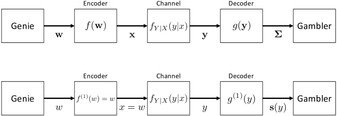
Figure 1: Depiction of the genie-gambler system. Top figure: General form of the system; bottom figure: single-letter code form of the system. In the single-letter code, we assume that the encoder is trivial, i.e., $x=f^{(1)}(w)=w$. Compare with the related figure [2, Fig. 1].

The communication channel from genie to gambler is depicted in the upper diagram in Figure 1, with components described formally as follows:

• Encoding and channel inputs: The genie has the list of winners $\mathbf{w}=[w_{1},w_{2},\ldots,w_{N}]\in(\mathcal{I}_{K})^{N}$. The genie also has an encoding function $f:(\mathcal{I}_{K})^{N}\rightarrow(\mathcal{I}_{K})^{N}$, and uses this function to generate and transmit channel inputs $\mathbf{x}$, given by

  $$\mathbf{x} =f(\mathbf{w})=[x_{1},x_{2},\ldots,x_{N}],$$ (9)

  where $\mathbf{x}\in(\mathcal{I}_{K})^{N}$.

• Channel outputs and decoding: The gambler prepares in advance a set of possible strategies $\mathcal{S}$, where each strategy $\mathbf{s}_{j}\in\mathcal{S}$ satisfies (1)-(2). The gambler observes channel outputs $\mathbf{y}=[y_{1},y_{2},\ldots,y_{N}]\in(\mathcal{I}_{K})^{N}$. The gambler also has a decoding function $g:(\mathcal{I}_{K})^{N}\rightarrow\mathcal{S}^{N}$ which maps channel outputs to strategies, and uses this function to determine her sequence of strategies

  $$\mathbf{\Sigma} =g(\mathbf{y})=[\mathbf{s}_{1},\mathbf{s}_{2},\cdots,\mathbf{s}_{N}],$$ (10)

  where $\mathbf{\Sigma}\in\mathcal{S}^{N}$.

• Channel input-output characteristics: Let $(x_{j},y_{j})$ represent the input-output pair for the $j$th race. The discrete channel is parameterized by the conditional input-output distribution $p_{Y|X}(y_{j}\>|\>x_{j})$.

• Channel uses: The channel can be used to send one symbol per race, and we assume the communication session occurs before the race, so $(x_{j},y_{j})$ may be used to inform the strategy $\mathbf{s}_{j}$ in race $j$. Channel uses are independent and identically distributed (IID).

II-C Growth rates

The per-race growth rate $\eta$ of the wealth $M_{j}$ can be written as a function of strategy $\mathbf{s}_{j}$ and winner $w_{j}$: $\eta(\mathbf{s}_{j},w_{j})=M_{j+1}/M_{j}$. From (4), this reduces to

$$\eta(\mathbf{s}_{j},w_{j}) =\sum_{i\in\mathcal{I}_{K}}s_{j}(i)r(i,w)$$ (11)

(cf. (7)). We are interested in the log rate of growth with respect to the sequence $\mathbf{\Sigma}$ of strategies

$$\Lambda(\mathbf{\Sigma}) =\frac{1}{N}\sum_{j=1}^{N}\log\eta(\mathbf{s}_{j},w_{j})=\frac{1}{N}\sum_{j=1}^{N}\log\sum_{i\in\mathcal{I}_{K}}s_{j}(i)r(i,w_{j}).$$ (12)

There are two special cases of the growth rate, and associated strategies, of interest:

• If the side information $y_{j}$ is perfect information (PI), i.e. $y_{j}=w_{j}$, the optimal strategy is to wager the entire fortune on the largest payoff for $w_{j}$. We write the optimal growth rate as $\Lambda^{\text{(PI)}\star}$, and the associated strategy at each time $j$ as $\mathbf{s}^{\text{(PI)}\star}(w_{j})$.

• If there is no side information (NSI), or the side information is uninformative, i.e. $y_{j}\perp w_{j}$, we write the optimal growth rate as $\Lambda^{\text{(NSI)}\star}$, and the associated strategy as $\mathbf{s}^{\text{(NSI)}\star}$.

In both of the above cases, the appropriate strategy is substituted into (12) in place of $\mathbf{s}_{j}$.

II-D Cost and Distortion

There may be a cost to acquire the side information $\mathbf{y}$. For the purposes of this paper, we assume that the cost is a per-race “commission” charged by the genie, depending on the expected fidelity of the side information that the genie provides. Let $\phi(w_{j},y_{j})$ represent the fidelity function for winner $w_{j}$ and side information $y_{j}$, where

$$\phi(w_{j},y_{j}) =\log\frac{p_{Y|W}(y_{j}\>|\>w_{j})}{p_{Y}(y_{j})}.$$ (13)

From the genie’s perspective, the fidelity depends only on $w_{j}$, which is known to the genie (while $y_{j}$ is not):

$$\phi(w_{j}) =E_{Y|W}\Big{[}\phi(w_{j},y_{j})\Big{]}$$ (14)

$$=D\Big{(}p_{Y|W}(\cdot\>|\>w_{j})\>||\>p_{Y}(\cdot)\Big{)},$$ (15)

where $D(\cdot\>||\>\cdot)$ is Kullback-Leibler divergence (cf. [2, Eqn. (9)]). Note that the expectation is taken over $y_{j}$ and not $w_{j}$. The genie then charges a commission on $\phi(w_{j})$, plus a constant cost of operating the channel, so the cost function $\rho(w_{j})$ is

$$\rho(w_{j}) =c_{1}\phi(w_{j})+\rho_{1}=c_{1}D\Big{(}p_{Y|W}(\cdot\>|\>w_{j})\>||\>p_{Y}(\cdot)\Big{)}+\rho_{1},$$ (16)

where $c_{1}$, the rate of the commission, is a positive constant, and $\rho_{1}$, the constant cost, is any real number. Define the average cost $\Gamma$ as

$$\Gamma =\frac{1}{N}\sum_{j=1}^{N}\rho(w_{j}).$$ (17)

There is clearly distortion in the genie-gambler channel. From Figure 1, distortion is measured between the sequences $\mathbf{w}$ and $\mathbf{\Sigma}$. We define distortion as the loss due to imperfect information using strategy sequence $\mathbf{\Sigma}$, compared with an optimal strategy with perfect knowledge of $\mathbf{w}$. Thus, distortion between these sequences is given by

$$\Delta =\Lambda^{(\text{PI})\star}-\Lambda(\mathbf{\Sigma})-\Gamma.$$ (18)

In our formulation, note that $\Gamma$ is part of the loss, as the gambler must pay for the information out of her winnings.

For a single race, the loss per race is the difference in $\eta$ between the best strategy with knowledge of the correct winner $w_{j}$ (i.e., $\mathbf{s}^{\text{(PI)}\star}(w_{j})$), and the strategy $\mathbf{s}_{j}$ arising from the side information $\mathbf{y}$, minus the cost of the information. We can write this loss as a function of $\mathbf{s}^{\text{(PI)}\star}(w_{j})$ and $\mathbf{s}_{j}$ (see (11)):

$$d\Big{(}\mathbf{s}^{\text{(PI)}\star}(w_{j}),\mathbf{s}_{j}\Big{)} =\log\eta\Big{(}\mathbf{s}^{\text{(PI)}\star}(w_{j}),w_{j}\Big{)}-\log\eta\Big{(}\mathbf{s}_{j},w_{j}\Big{)}-\rho(w_{j})$$ (19)

$$=\log\sum_{i\in\mathcal{I}_{K}}s^{\text{(PI)}\star}(w_{j},i)r(i,w_{j})-\log\sum_{i\in\mathcal{I}_{K}}s_{j}(i)r(i,w_{j})-\rho(w_{j})$$ (20)

$$\triangleq d(w_{j},\mathbf{s}_{j}),$$ (21)

Returning to (18), it should be clear that

$$\Delta =\frac{1}{N}\sum_{j=1}^{N}d(w_{j},\mathbf{s}_{j}).$$ (22)

We define $d(w_{j},\mathbf{s}_{j})$ as the distortion function for our system. A similar distortion function was used by Erkip and Cover [5].

II-E Single-letter codes

Suppose there exist functions $f^{(1)}:\mathcal{I}_{K}\rightarrow\mathcal{I}_{K}$ and $g^{(1)}:\mathcal{I}_{K}\rightarrow\mathcal{S}$ such that (9) and (10) can be written

$$\mathbf{x}=f(\mathbf{w}) =[x_{1},x_{2},\ldots,x_{N}]$$ (23)

$$=[f^{(1)}(w_{1}),f^{(1)}(w_{2}),\ldots,f^{(1)}(w_{N})]$$ (24)

$$\mathbf{\Sigma}=g(\mathbf{y}) =[\mathbf{s}_{1},\mathbf{s}_{2},\cdots,\mathbf{s}_{N}]$$ (25)

$$=[g^{(1)}(y_{1}),g^{(1)}(y_{2}),\ldots,g^{(1)}(y_{N})].$$ (26)

A code with encoder and decoder satisfying properties (24) and (26), respectively, is called a single-letter code.

From this point onward we will focus on single-letter code strategies. Since channel uses are IID, when discussing single-letter codes we will drop the time subscripts where it is unambiguous to do so (e.g., $x_{j}$ becomes $x$). We will also assume that the encoder is trivial, so that

$$x=f^{(1)}(w)=w.$$ (27)

Furthermore, since strategy $\mathbf{s}=g^{(1)}(y)$ is a function of only a single channel output $y$, we will make the dependence explicit and write the strategy vector as

$$\mathbf{s}(y)=\Big{[}s(y,1),s(y,2),\ldots,s(y,K)\Big{]}$$ (28)

(cf. (6)), i.e., $g^{(1)}(y)=\mathbf{s}(y)$. Similarly, when referring to single-letter codes, we will simplify the distortion function’s notation to $d(w,y)$, where

$$d(w,y) \triangleq d(w,\mathbf{s}(y)).$$ (29)

Our system, with the single-letter code notation, is depicted in the lower diagram of Figure 1.

With a single-letter code, the set of possible strategies is simplified to

$$\mathcal{S}=\Big{\{}\mathbf{s}(y):y\in\mathcal{I}_{K}\Big{\}},$$ (30)

one strategy per output letter. Since $y\in\mathcal{I}_{K}$, the strategies can also be represented in a $K\times K$ strategy matrix $\mathbf{S}$, where

$$\mathbf{S} =\left[\begin{array}[]{c}\mathbf{s}(1)\\ \mathbf{s}(2)\\ \vdots\\ \mathbf{s}(K)\end{array}\right].$$ (35)

Define a valid strategy matrix as follows:

Definition.

A $K\times K$ matrix $\mathbf{S}$ is a valid strategy matrix if and only if its rows satisfy (1)-(2); equivalently, if and only if it is row stochastic.

The following example connects our model and notation to classic Kelly betting.

Example 1  (Kelly betting with two horses): Here we restate the scenario from the introduction in the notation defined above. Suppose $K=2$, and each horse can win with equal probability: $p_{W}(1)=p_{W}(2)=\frac{1}{2}$. Winning bets pay double while losing bets pay nothing, yielding a reward matrix

$$\mathbf{R} =\begin{bmatrix}2&0\\ 0&2\end{bmatrix},$$ (36)

and it can be checked that $\mathbf{R}$ is a valid reward matrix. The genie uses the trivial encoder $x=f^{(1)}(w)=w$. The gambler observes $y$ through the genie-gambler channel, which is a binary symmetric channel with error probability $q$. That is, for $x,y\in\{1,2\}$,

$$p_{Y|X}(y\>|\>x) =\left\{\begin{array}[]{cl}1-q,&x=y\\ q,&x\neq y.\end{array}\right.$$ (39)

The set of possible strategies $\mathcal{S}$ consists of

$$\mathcal{S} =\Big{\{}[1-q,q],[q,1-q]\Big{\}},$$ (40)

and the decoder is given by

$$\mathbf{s}(y)=g^{(1)}(y) =\left\{\begin{array}[]{cl}\>[1-q,q],&y=1,\\ \>[q,1-q],&y=2.\end{array}\right.$$ (43)

The strategies can be arranged in a strategy matrix

$$\mathbf{S} =\begin{bmatrix}1-q&q\\ q&1-q\end{bmatrix},$$ (44)

which is row stochastic and thus a valid strategy matrix. It can be seen that this example is identical to Kelly’s scheme [1]. $\triangle$

II-F Optimality of single-letter codes

Coding schemes have cost-distortion pairs given by $(\Gamma,\Delta)$. Whether single-letter or not, a code is optimal given $d(w,\mathbf{s})$ and $\rho(w)$ if no other code can reduce $\Delta$ for the same $\Gamma$, nor reduce $\Gamma$ for the same $\Delta$ [2, Defn. 5]. In our terms, an optimal scheme is one where the gambler can’t increase her return without paying the genie more for the information, nor can she get away with paying less for the same return.

From [2, Thm. 6], a single-letter code is optimal if and only if the following conditions on the distortion and cost function simultaneously hold:

• In terms of the distortion function $d(w,y)$, if $I(W;Y)>0$, then

  $$d(w,y)=-c\log{}p_{W|Y}(w\>|\>y)+d_{0}(w),$$ (45)

  where $c$ is any positive constant, and $d_{0}(w)$ is any function of $w$. If $I(W;Y)=0$, then $d(w,y)$ can be any function.

• In terms of the cost function $\rho(w)$, if $I(X;Y)<C$ (for Shannon capacity $C$), then

  $$\rho(w)=c_{1}D\big{(}p_{Y|W}(\cdot|w)||p_{Y}(\cdot)\big{)}+\rho_{1},$$ (46)

  where $c_{1}$ is any positive constant, and $\rho_{1}$ is any constant, positive or not. If $I(X;Y)=C$, then $\rho(w)$ can be any function.

Comparing (46) to (16), it should be clear that the cost function $\rho(w)$ is selected to always satisfy this criterion. Our focus in this paper is on the distortion function, and we will seek solutions where distortion is minimized (i.e., $\min\Delta$).

III Results for diagonal reward matrices

A reward matrix $\mathbf{R}$ is diagonal if $r(i,j)=0\>\forall\>i\neq j$. Diagonal reward matrices are valid if and only if all diagonal elements are strictly positive.

Here we give our main results for diagonal matrices, where a bet on a losing horse pays nothing. While these results demonstrate the optimality of single letter codes for classic Kelly betting, we show in Section IV that these approaches are also useful when $\mathbf{R}$ is nondiagonal.

III-A Diagonal reward matrices, side information, and proportional betting

If $\mathbf{R}$ is diagonal, then the log growth rates have simple forms, which we introduce in this section. While these derivations are straightforward, they are useful to the remainder of the exposition, particularly the proportional betting strategy.

For diagonal $\mathbf{R}$, strategy matrix $\mathbf{S}$, channel observation $y$, and winner $w$, as $N\rightarrow\infty$ (12) simplifies to

$$\Lambda_{\text{diag.}}(\mathbf{S}) =E\Bigg{[}\log\Big{(}s(y,w)r(w,w)\Big{)}\Bigg{]}$$ (47)

$$=\sum_{y\in\mathcal{I}_{K}}\sum_{w\in\mathcal{I}_{K}}p_{W}(w)p_{Y|X}(y|w)\log\Big{(}s(y,w)r(w,w)\Big{)},$$ (48)

where $p_{W}(w)$ is the prior distribution on the winners, and $p_{Y|X}(y|w)$ the channel conditional input-output probability, assuming the trivial encoder from (27). The optimal strategies and mean log growth rates are given as follows.

Perfect information: When $y=w$, the optimal strategy $\mathbf{s}^{\text{(PI)}\star}(w)$ is simply

$$s^{\text{(PI)}\star}(w,i)=\delta_{iw},$$ (49)

i.e., the entire fortune is wagered on the known winner. The optimal growth rate is then

$$\Lambda_{\text{diag.}}^{(\text{PI})\star}=\sum_{w\in\mathcal{I}_{K}}p_{W}(w)\log r(w,w).$$ (50)

(For non-diagonal $\mathbf{R}$, (49) is not necessarily the optimal strategy; for an example, see (103) below.)

Noisy side information: Given $y$, the optimal strategy performs conditional proportional betting using the a posteriori distribution, that is,

$$s^{\star}(y,i) =p_{W|Y}(i\>|\>y)$$ (51)

Substituting (51) into (48) yields an optimal growth rate

$$\Lambda_{\text{diag.}}^{\star} =\sum_{y\in\mathcal{I}_{K}}\sum_{w\in\mathcal{I}_{K}}p_{W}(w)p_{Y|X}(y|w)\log\Big{(}p_{W|Y}(w\>|\>y)r(w,w)\Big{)}$$ (52)

$$=\sum_{w\in\mathcal{I}_{K}}p_{W}(w)p_{Y|X}(y|w)\log p_{W|Y}(w\>|\>y)+\sum_{w\in\mathcal{I}_{K}}p_{W}(w)\log r(w,w)$$ (53)

$$=\Lambda_{\text{diag.}}^{(\text{PI})\star}-H(W|Y).$$ (54)

Note that (50) is consistent with (54) since perfect side information implies $H(W|Y)=0$.

For proportional betting, the strategy matrix is written

$$\mathbf{S}^{\star}=\mathbf{P}_{W|Y} \triangleq\left[\begin{array}[]{cccc}p_{W|Y}(1\>|\>1)&p_{W|Y}(2\>|\>1)&\cdots&p_{W|Y}(K\>|\>1)\\ p_{W|Y}(1\>|\>2)&p_{W|Y}(2\>|\>2)&\cdots&p_{W|Y}(K\>|\>2)\\ \vdots&\vdots&\ddots&\vdots\\ p_{W|Y}(1\>|\>K)&p_{W|Y}(2\>|\>K)&\cdots&p_{W|Y}(K\>|\>K)\\ \end{array}\right],$$ (59)

in which the $y$th row of $\mathbf{S}^{\star}$ is $\mathbf{s}^{\star}(y)$.

No side information: If $w$ and $y$ are independent, then $p_{W|Y}(w\>|\>y)=p_{W}(w)$. Following (51), the optimal strategy is again proportional betting, but this time with respect to the a priori distribution

$$s(y,w) =p_{W}(w).$$ (60)

Following a derivation similar to (52)-(54), we have

$$\Lambda_{\text{diag.}}^{(\text{NSI})\star} =\Lambda_{\text{diag.}}^{(\text{PI})\star}-H(W).$$ (61)

Illustrating these growth rates, we give the following example.

Example 2  (Kelly betting with fair odds): Suppose $\mathbf{R}$ is diagonal, and fair odds are given: $r(w,w)=(p_{W}(w))^{-1}$. Then from (50), (54), and (61),

$$\Lambda_{\text{diag.}}^{(\text{PI})\star} =\sum_{w\in\mathcal{I}_{K}}p_{W}(w)\log\frac{1}{p_{W}(w)} =H(W)$$ (62)

$$\Lambda_{\text{diag.}}^{\star} =H(W)-H(W\>|\>Y) =I(W;Y)$$ (63)

$$\Lambda_{\text{diag.}}^{\text{(NSI)}\star} =H(W)-H(W) =0.$$ (64)

We apply this observation to the two-horse Kelly betting scheme in Example Definition. Since the winners are equiprobable ($p_{W}(1)=p_{W}(2)=\frac{1}{2}$), the reward matrix (36) gives fair odds. It can be checked that the strategy matrix $\mathbf{S}^{\star}$ in (44) satisfies (51). Finally, if $\mathscr{H}(p)\triangleq-p\log p-(1-p)\log(1-p)$ is the binary entropy function, then $\Lambda_{\text{diag.}}^{\star}=1-\mathscr{H}(p)$. Note that the optimal growth rate $\Lambda_{\text{diag.}}^{\star}$ is the Shannon capacity $C$ of this genie-gambler channel. $\triangle$

III-B Distortion

With diagonal $\mathbf{R}$, the distortion function from Section II-D can be simplified. Following (19)-(21), the return per race is given by

$$\eta\Big{(}\mathbf{s}^{\text{(PI)}\star}(w),w\Big{)} =r(w,w)$$ (65)

for perfect side information, and

$$\eta\Big{(}\mathbf{s}(y),w\Big{)} =s(y,w)r(w,w)$$ (66)

for noisy side information. Thus,

$$d(w,y) =\log\eta\Big{(}\mathbf{s}^{\text{(PI)}\star}(w),w\Big{)}-\log\eta\Big{(}\mathbf{s}(y),w\Big{)}-\rho(w)$$ (67)

$$=\log r(w,w)-\log s(y,w)r(w,w)-\rho(w)$$ (68)

$$=-\log s(y,w)-\rho(w).$$ (69)

Using the proportional betting strategy matrix $\mathbf{S}^{\star}$, which is optimal, from (59) we have

$$d(w,y) =-\log p_{W|Y}(w\>|\>y)-\rho(w).$$ (70)

III-C Optimal Kelly betting with single-letter codes

We are now ready to state our main result for diagonal matrices.

Theorem 1.

Let $\mathbf{R}$ be a valid diagonal strategy matrix, let the distortion function $d(w,y)$ be given by (20), and suppose the cost function $\rho(w)$ satisfies (46). If the gambler uses the proportional betting strategy $\mathbf{S}^{\star}=\mathbf{P}_{W|Y}$, then the genie-gambler channel admits an optimal single-letter code, with encoder $f^{(1)}(w)=w$ and decoder $g^{(1)}(y)=\mathbf{s}^{\star}(y)$, where $\mathbf{s}^{\star}(y)$ are the rows of $\mathbf{S}^{\star}=\mathbf{P}_{W|Y}$ in (59).

Proof.

The result is an application of [2, Thm. 6]. Since (70) satisfies (45) with $c=1$ and $d_{0}(w)=\rho(w)$, the distortion criterion is satisfied. Meanwhile, (46) is satisfied by assumption. Thus, an optimal single-letter code is available using strategy $\mathbf{S}^{\star}$ for $\mathbf{R}$. ∎

Theorem 1 demonstrates that, for any diagonal $\mathbf{R}$, single-letter codes are sufficient to achieve the best log rate of return (i.e., $\min\Delta$) of any possible scheme with fixed cost $\Gamma$, whether or not complicated signal processing is employed. Moreover, from (63), if fair odds are given, this optimal rate of return is $\Lambda_{\text{diag.}}^{\star}=I(W;Y)$.

IV Results for non-diagonal reward matrices

For diagonal $\mathbf{R}$, the general distortion function (19)-(20) reduces to a simplified form (68) with a single term under each sum. This simplification is no longer possible with non-diagonal reward matrices. In this section, we develop tools to deal with this complication.

In a horse race with a non-diagonal $\mathbf{R}$, gamblers may receive rewards for betting on a losing horse. Although this might not be the way most racetracks work, there are many physical and economic motivations for non-diagonal $\mathbf{R}$. The type of reward matrix we consider here is analogous to a fitness matrix in evolutionary biology, with each component describing the expected number of offspring an individual expressing a particular phenotype will produce in a particular environmental state. In this context, several studies have built upon the concept of fitness sets [21] to develop a decomposition of the fitness matrix in terms of specialized hypothetical phenotypes [22, 8]. The results in this section consider proportional betting over those hypothetical phenotypes.

IV-A Reward matrix decomposition

Our general approach is to decompose a non-diagonal reward matrix $\mathbf{R}$ into a product of two matrices, where one is diagonal, and the other is row stochastic. The diagonal matrix is then an effective reward matrix for an equivalent race with hypothetical “horses”, while the row stochastic matrix transforms the actual strategy $\mathbf{S}$ into an effective strategy over those horses. We can then use an approach similar to that in Theorem 1 on the effective reward matrix.

In the remainder of this section we give two lemmas that establish the existence and properties of this decomposition. A similar approach was taken in [8], which we extend and formalize in the results below.

Lemma 2.

Suppose $\mathbf{R}$ is a valid reward matrix. Let

$$\mathbf{q}=\mathbf{R}^{-1}\vec{1}.$$ (71)

If and only if

$$q_{i}>0\>\>\forall i,$$ (72)

then there exists a decomposition

$$\mathbf{R}=\mathbf{B}\mathbf{D},$$ (73)

where $\mathbf{B}$ is a row stochastic matrix, and $\mathbf{D}$ is a valid diagonal reward matrix given by

$$\mathbf{D}=\Big{(}{\,\mathrm{diag}}(\mathbf{R}^{-1}\vec{1})\Big{)}^{-1}.$$ (74)

Proof.

The proof is found in Appendix -A. ∎

The following lemma establishes that we can manipulate the strategy and reward matrices under decomposition, while preserving important properties both of these matrices and of the distortion function.

Lemma 3.

Let $\mathbf{S}$ be a valid strategy matrix, let $\mathbf{D}$ be a valid diagonal reward matrix, let $\mathbf{B}$ be any row-stochastic matrix, and let $\mathbf{R}=\mathbf{B}\mathbf{D}$. Then:

1. $\mathbf{T}=\mathbf{S}\mathbf{B}$ is a valid strategy matrix;

2. Letting $d_{\mathbf{S},\mathbf{R}}(w,y)$ represent the distortion using strategy matrix $\mathbf{S}$ and reward matrix $\mathbf{R}$ (cf. (20)), there exists a function $\psi(w)$ such that $d_{\mathbf{S},\mathbf{R}}(w,y)=d_{\mathbf{T},\mathbf{D}}(w,y)+\psi(w)$; and

3. If $\mathbf{T}$ is the optimal ($\min\Delta$) strategy matrix for $\mathbf{D}$, then $\mathbf{S}$ is the optimal strategy matrix for $\mathbf{R}$.

Proof.

The proof is found in Appendix -B. ∎

IV-B Effective and actual strategies

In Lemma 3 we introduced $\mathbf{T}=\mathbf{S}\mathbf{B}$, and we now define $\mathbf{T}$ as the effective strategy matrix with rows $\mathbf{t}(y)$, analogous to $\mathbf{s}(y)$. From the lemma, $\mathbf{T}$ is a valid strategy matrix.

Since $\mathbf{D}$ is diagonal, and since we can manipulate the reward and strategy matrices, it appears that Theorem 1 holds if condition (72) holds, and if we set $\mathbf{T}^{\star}=\mathbf{P}_{W|Y}$ to implement proportional betting, satisfying (51). However, it is the validity of the actual strategy $\mathbf{S}$ that determines whether a single-letter code is optimal: bets are taken on actual horses, not effective ones. That is, we want to set $\mathbf{S}^{\star}=\mathbf{T}^{\star}\mathbf{B}^{-1}$, but it is possible that $\mathbf{S}^{\star}$ is not valid, meaning the optimal effective strategy $\mathbf{T}^{\star}$ is not achieved by any actual strategy. (This issue is avoided in Lemma 3 by restricting the results to valid $\mathbf{S}$.)

As an illustration of the issue, consider the following example.

Example 3  (Valid and invalid strategies under decomposition): Consider the non-diagonal reward matrix

$$\mathbf{R} =\left[\begin{array}[]{cc}2&1\\ 1&3\end{array}\right].$$ (77)

The decomposition in (73) exists, with

$$\mathbf{B} =\mathbf{R}\mathbf{D}^{-1}=\left[\begin{array}[]{cc}2&1\\ 1&3\end{array}\right]\left[\begin{array}[]{cc}2/5&0\\ 0&1/5\end{array}\right]=\left[\begin{array}[]{cc}4/5&1/5\\ 2/5&3/5\end{array}\right].$$ (84)

Given an effective strategy $\mathbf{T}$, we want to find the corresponding real strategy $\mathbf{S}=\mathbf{T}\mathbf{B}^{-1}$, so we need

$$\mathbf{B}^{-1} =\left[\begin{array}[]{cc}3/2&-1/2\\ -1&2\end{array}\right].$$ (87)

Consider a row $\mathbf{t}(y)=[t,1-t]$ from $\mathbf{T}$. The corresponding real strategy is $\mathbf{s}(y)=\mathbf{t}(y)\mathbf{B}^{-1}$, i.e., $\mathbf{s}(y)=\left[\frac{5t}{2}-1,2-\frac{5t}{2}\right]$. It can be checked that $\mathbf{s}(y)$ is a valid strategy if and only if $2/5\leq t\leq 4/5$.

Now suppose the genie-gambler channel is a binary symmetric channel with crossover probability $p=2/5$, and suppose the horses are equally likely to win a priori: $p_{W}(1)=p_{W}(2)=1/2$. Then $p_{W|Y}(w\>|\>y)=3/5$ for $w=y$, and $2/5$ for $w\neq y$. From (59), the optimal effective strategy matrix $\mathbf{T}^{\star}$ is given by proportional betting as

$$\mathbf{T}^{\star}=\mathbf{P}_{W|Y} =\left[\begin{array}[]{cc}3/5&2/5\\ 2/5&3/5\end{array}\right].$$ (90)

From Lemma 3, since $\mathbf{T}^{\star}$ is optimal for $\mathbf{D}$, then $\mathbf{S}^{\star}=\mathbf{T}^{\star}\mathbf{B}^{-1}$ is optimal for $\mathbf{R}$ (as long as it is valid), that is,

$$\mathbf{S}^{\star} =\left[\begin{array}[]{cc}1/2&1/2\\ 0&1\end{array}\right].$$ (93)

In this case, $\mathbf{S}^{\star}$ is row-stochastic, and is thus a valid strategy matrix.

However, if $p<2/5$, it can be checked that some elements of $\mathbf{S}^{\star}$ are negative, so the strategy matrix is not valid. In this case, an effective proportional betting strategy $\mathbf{T}^{\star}=\mathbf{P}_{W|Y}$ is not achievable by any actual strategy $\mathbf{S}$. $\triangle$

IV-C Single-letter codes and general reward matrices

With the issue from Example IV-B in mind, we can state our main result for general $\mathbf{R}$.

Theorem 4.

Let $\mathbf{R}$ be a valid reward matrix, let $d(w,y)$ be given by (20), and let $\rho(w)$ be a cost function satisfying (46). If the decomposition $\mathbf{R}=\mathbf{B}\mathbf{D}$ from (73) exists, and if $\mathbf{S}^{\star}=\mathbf{P}_{W|Y}\mathbf{B}^{-1}$ is a valid strategy matrix, then an optimal single-letter code exists for $\mathbf{R}$, with encoder $f^{(1)}(w)=w$ and decoder $g^{(1)}(y)=\mathbf{s}^{\star}(y)$, where $\mathbf{s}^{\star}(y)$ are the rows of $\mathbf{S}^{\star}$.

Proof.

From Lemma 2, if the decomposition (73) exists, then $\mathbf{D}$ is a valid diagonal reward matrix.

From Theorem 1, $\mathbf{T}^{\star}=\mathbf{P}_{W|Y}$ is the optimal strategy matrix for any diagonal reward matrix $\mathbf{D}$, and an optimal single-letter code exists for a system with distortion function $d_{\mathbf{T}^{\star},\mathbf{D}}(w,y)$ (in the notation of Lemma 3) and cost function $\rho(w)$.

It remains to show that the distortion criterion is satisfied for the non-diagonal $\mathbf{R}$. From Lemma 3, since $\mathbf{S}^{\star}$ is (by presupposition) a valid strategy matrix, and since $\mathbf{T}^{\star}=\mathbf{P}_{W|Y}$ is the optimal ($\min\Delta$) strategy matrix for $\mathbf{D}$, then $\mathbf{S}^{\star}$ is optimal for $\mathbf{R}$. Further, if $d_{\mathbf{T}^{\star},\mathbf{D}}(w,y)$ is the distortion function satisfying Theorem 1 (in the notation of the lemma), then

$$d_{\mathbf{S}^{\star},\mathbf{R}}(w,y) =d_{\mathbf{T}^{\star},\mathbf{D}}(w,y)+\psi(w)$$ (94)

$$=-\log p_{W|Y}(w\>|\>y)-\rho(w)+\psi(w).$$ (95)

The distortion criterion $d_{\mathbf{S}^{\star},\mathbf{R}}(w,y)$ satisfies (45) with $c=1$ and $d_{0}(w)=-\rho(w)+\psi(w)$. Thus, there exists an optimal single letter code for $\mathbf{R}$ with the given encoder and decoder. ∎

While Theorem 1 showed that Kelly betting on diagonal reward matrices was optimal with uncoded side information, Theorem 4 extends the result to a subset of nondiagonal reward matrices $\mathbf{R}$ (namely, those that can be decomposed into $\mathbf{R}=\mathbf{B}\mathbf{D}$), and subjects it to conditions on the side information (namely, that $\mathbf{P}_{W|Y}\mathbf{B}^{-1}$ is a row-stochastic matrix, which permits proportional betting over $\mathbf{D}$). Indeed, if $\mathbf{R}$ is already diagonal, then the decomposition $\mathbf{R}=\mathbf{B}\mathbf{D}$ exists with $\mathbf{B}=\mathbf{I}$, and Theorem 1 can be obtained as a special case of Theorem 4. Moreover, proportional betting is always available for diagonal $\mathbf{R}$, because there is no difference between the effective and actual strategy.

It is worth noting that, as the side information gets better, it normally becomes more difficult to satisfy the requirement that $\mathbf{P}_{W|Y}\mathbf{B}^{-1}$ is row stochastic. This was seen implicitly in Example IV-B, but can also be seen as follows. Suppose the side information is perfectly informative, so that $\mathbf{P}_{W|Y}=\mathbf{I}$. Then $\mathbf{S}^{\star}=\mathbf{P}_{W|Y}\mathbf{B}^{-1}=\mathbf{I}\mathbf{B}^{-1}=\mathbf{B}^{-1}$. However, the inverse of a row stochastic matrix is not row stochastic except in special cases, so $\mathbf{S}^{\star}$ is not generally valid in this scenario.

IV-D Two-horse races

For two-horse races, we can give the conditions in Theorem 4 explicitly. Consider first the existence of decomposition (73) for $2\times 2$ reward matrices:

$$\mathbf{R}=\begin{bmatrix}r(1,1)&r(1,2)\\ r(2,1)&r(2,2)\end{bmatrix}=\begin{bmatrix}r_{11}&r_{12}\\ r_{21}&r_{22}\end{bmatrix}$$ (96)

where the notation on the right is used for brevity. Considering Lemma 2, we obtain $\mathbf{q}=\mathbf{R}^{-1}\vec{1}$, which gives

$$\mathbf{q}=\begin{bmatrix}q_{1}\\ q_{2}\end{bmatrix}=\begin{bmatrix}\frac{r_{22}-r_{12}}{r_{11}r_{22}-r_{12}r_{21}}\\ \frac{r_{11}-r_{21}}{r_{11}r_{22}-r_{12}r_{21}}\end{bmatrix}.$$ (97)

In order for decomposition (73) to exist, we require that the elements of $\mathbf{q}$ are positive. Considering each term at a time, we consider the cases where either $q_{1}\leq 0$ or $q_{2}\leq 0$, i.e., the decomposition does not exist:

• $q_{1}$: If $r_{12}=r_{22}$, then $q_{1}=0$, and the decomposition does not exist. Otherwise, for $q_{1}<0$, the numerator and denominator have different signs. The numerator is clearly positive if $r_{12}<r_{22}$ and negative if $r_{12}>r_{22}$. The denominator is positive if $r_{12}<\frac{r_{11}}{r_{21}}r_{22}$, and negative if $r_{12}>\frac{r_{11}}{r_{21}}r_{22}$. Thus, both are positive if $r_{12}<\min\{1,\frac{r_{11}}{r_{21}}\}r_{22}$, and both are negative if $r_{12}>\max\{1,\frac{r_{11}}{r_{21}}\}r_{22}$. Conversely, $q_{1}<0$ if and only if

  $$\frac{r_{12}}{r_{22}}\in\left(\min\left\{1,\frac{r_{11}}{r_{21}}\right\},\max\left\{1,\frac{r_{11}}{r_{21}}\right\}\right).$$ (98)

• $q_{2}$: By a similar argument, if $r_{11}=r_{21}$, then $q_{2}=0$; moreover, $q_{2}<0$ if and only if

  $$\frac{r_{21}}{r_{11}}\in\left(\min\left\{1,\frac{r_{22}}{r_{12}}\right\},\max\left\{1,\frac{r_{22}}{r_{12}}\right\}\right).$$ (99)

We also give the following definition: a reward matrix $\mathbf{R}$ has a dominant wager if there exists $i\in\mathcal{I}_{K}$ such that

$$r(i,w) \geq r(k,w)\>\>\>\>\forall k\in\mathcal{I}_{K},w\in\mathcal{I}_{K}.$$ (100)

That is, betting on $i$ gives the same or better return than any other bet, regardless of the winner. For example, the reward matrix

$$\mathbf{R} =\left[\begin{array}[]{cc}4&3\\ 1&2\end{array}\right]$$ (103)

has a dominant wager of $i=1$: the first row contains the largest element in any column, even though (8) is satisfied. In an $\mathbf{R}$ with a dominant wager, the optimal strategy is to ignore the side information and always bet the entire fortune on the dominant wager: for $\mathbf{R}$ as in (103), the optimal strategy matrix $\mathbf{S}^{\star}$ is

$$\mathbf{S}^{\star} =\left[\begin{array}[]{cc}1&0\\ 1&0\end{array}\right].$$ (106)

The existence of the decomposition, and its consequences, are summarized in the following lemma.

Lemma 5.

For a valid $2\times 2$ reward matrix $\mathbf{R}$:

1. The decomposition in (73) exists if and only if either $r_{12}<r_{22}$ and $r_{21}<r_{11}$, or $r_{12}>r_{22}$ and $r_{21}>r_{11}$.

2. If the decomposition in (73) does not exist, then $\mathbf{R}$ has a dominant wager.

Proof.

The proof is given in Appendix -C. ∎

Systems with dominant wagers always admit trivial single-letter codes with rate zero, as there is no need to communicate at all in order to achieve optimal $\Delta$. Fitting this into the framework from [2], the genie can notionally use an encoder that only encodes a single source symbol, representing the single desirable horse. For such an encoder, the mutual information between source and representation is zero, and a trivial optimal single-letter code exists; see part (iii) of [2, Thm. 6].

We now consider the effective and actual strategies when the decomposition exists. The optimal effective strategy matrix is written as

$$\mathbf{T}^{\star}\triangleq\begin{bmatrix}\alpha^{\star}&1-\alpha^{\star}\\ 1-\beta^{\star}&\beta^{\star}\end{bmatrix}=\mathbf{S}^{\star}\mathbf{B},$$ (107)

and if the proportional betting solution is available, then $\mathbf{T}^{\star}=\mathbf{P}_{W|Y}$. For a $2\times 2$ reward matrix it is straightforward to explicitly find $\mathbf{S}^{\star}$:

$$\mathbf{S}^{\star}=\mathbf{T}^{\star}\mathbf{B}^{-1}=\begin{bmatrix}\frac{\alpha^{\star}r_{22}}{r_{22}-r_{12}}+\frac{(1-\alpha^{\star})r_{21}}{r_{21}-r_{11}}&\frac{(1-\alpha^{\star})r_{11}}{r_{11}-r_{21}}+\frac{\alpha^{\star}r_{12}}{r_{12}-r_{22}}\\ \frac{(1-\beta^{\star})r_{22}}{r_{22}-r_{12}}+\frac{\beta^{\star}r_{21}}{r_{21}-r_{11}}&\frac{\beta^{\star}r_{11}}{r_{11}-r_{21}}+\frac{(1-\beta^{\star})r_{12}}{r_{12}-r_{22}}\end{bmatrix}$$ (108)

which has row sums equal to one but possibly has negative entries. Solving for $\mathbf{S}^{\star}\geq{}0$, the following conditions must be satisfied, consistent with the conditions in (8) for valid $\mathbf{R}$, and Lemma 5 for the existence of the decomposition:

$$\frac{r_{21}(r_{22}-r_{12})}{\det{\mathbf{R}}}\leq\alpha^{\star}\leq\frac{r_{11}(r_{22}-r_{12})}{\det{\mathbf{R}}}$$ (109)

$$\frac{r_{12}(r_{11}-r_{21})}{\det{\mathbf{R}}}\leq\beta^{\star}\leq\frac{r_{22}(r_{11}-r_{21})}{\det{\mathbf{R}}}.$$ (110)

If the conditions in (109)-(110) hold, then $\mathbf{S}^{\star}$ exists for the given $\mathbf{T}^{\star}$. We can now write the following result for two-horse races:

Proposition 6.

For a valid $2\times 2$ reward matrix $\mathbf{R}$:

1. If the decomposition (73) exists and (109)-(110) are satisfied, then an optimal single-letter code exists with optimal strategy $\mathbf{S}^{\star}=\mathbf{P}_{W|X}\mathbf{B}^{-1}$.

2. If the decomposition (73) does not exist, then the optimal distortion can be achieved with a trivial rate-zero single-letter code (i.e., without side information).

Proof.

The derivation leading up to (109)-(110) establishes that $\mathbf{S}^{\star}$ is a valid strategy if these conditions hold. The first part of the proposition then follows from Theorem 4. The second part of the proposition follows from Lemma 5 and part (iii) of [2, Thm. 6]. ∎

Proposition 6 leaves open the question of what happens when decomposition (73) exists, but (109)-(110) are not satisfied. In this case, proportional betting over $\mathbf{D}$ is not possible. This case is addressed in the next section.

V Beyond proportional betting

In the preceding results, we focused on strategies that resulted in proportional betting on the (effective) diagonal reward matrix: that is, we pursued only the classic Kelly bet of $s(y,w)=p_{W|Y}(w\>|\>y)$, or the effective bet $t(y,w)=p_{W|Y}(w\>|\>y)$. In Theorems 1 and 4, we showed that this strategy satisfies the Gastpar criterion (45) with $c=1$.

However, we have also seen that the proportional betting strategy is not always available for non-diagonal $\mathbf{R}$. In these cases we may ask: can (45) nonetheless be satisfied with $c\neq 1$? In this section, we answer this question in the affirmative, and give detailed results for $2\times 2$ reward matrices.

V-A Alternative solutions to (45)

We first show the existence of valid strategies satisfying $c\neq 1$. Note that the distortion criterion (45) can be rewritten

$$2^{-d(w,y)} =\Big{(}p_{W|Y}(w\>|\>y)\Big{)}^{c}2^{-d_{0}(w)}.$$ (111)

A given distortion function $d(w,y)$ satisfying (111) (or (45)) can be extended to a family of other distortion functions, as shown in the following minor lemma:

Lemma 7.

If $d(w,y)$ satisfies (111), then for any function $\psi(w)$, $d(w,y)+\psi(w)$ also satisfies (111).

Proof.

$$2^{-d(w,y)-\psi(w)} =2^{-d(w,y)}2^{-\psi(w)}$$ (112)

$$=\Big{(}p_{W|Y}(w\>|\>y)\Big{)}^{c}2^{-d_{0}(w)-\psi(w)},$$ (113)

where (113) follows from (111). Then (111) is satisfied with constant $c$ and function $d_{0}(w)+\psi(w)$. ∎

We will use Lemma 7 to look for solutions while disregarding the cost function (i.e., with $\rho(w)=0$). If a solution exists, then we can use the lemma to ensure that a solution exists with the correct $\rho(w)$ added.

Now we may consider whether $c=1$ is the only possible setting. Let $\rho(w)=0$, and define the matrix

$$\mathbf{F}\triangleq\begin{bmatrix}2^{-d_{0}(1)}&\dots&0\\ \vdots&\ddots&\vdots\\ 0&\dots&2^{-d_{0}(K)}\end{bmatrix}.$$ (114)

Further let

$$\mathbf{Q}(c) \triangleq(\mathbf{P}_{W|Y})^{\circ{}c},$$ (115)

with the superscript $\circ{}c$ indicating the $c$th Hadamard power (i.e., elementwise power) of the matrix, and with $\mathbf{P}_{W|Y}$ given in (59).

Suppose $\mathbf{R}$ is diagonal and $\rho(w)=0$, so that $d(w,y)=-\log s(y,w)$ (see (69)). Then $2^{-d(w,y)}=s(y,w)$, and a solution satisfying (111) must have

$$\mathbf{S}=\mathbf{Q}(c)\mathbf{F}.$$ (116)

A viable strategy matrix must be row-stochastic, so we must find conditions under which $\mathbf{Q}(c)\mathbf{F}$ is row-stochastic. The choice of

$$\mathbf{F}\vec{1}=\mathbf{Q}(c)^{-1}\vec{1}$$ (117)

guarantees that $\mathbf{S}$ will have row sums equal to one, however $\mathbf{F}$ must have all positive diagonal components as they are exponential functions of $d_{0}(x)$. We now prove the existence of other viable choices of $c$ by showing that $\mathbf{Q}(c)^{-1}\vec{1}>0$ for some $c\neq{}1$.

Theorem 8.

Suppose $\mathbf{Q}(1)$ is nonsingular. Then:

1. Setting $\rho(w)=0$, there exists a neighborhood $B_{\delta}(c=1)$ for some $\delta>0$ such that if $c^{\prime}\in{}B_{\delta}(c=1)$, then the solution $\mathbf{Q}(c^{\prime})^{-1}\vec{1}=\mathbf{F}\vec{1}>0$.

2. The settings of $c^{\prime}$ from part 1 form a distortion function satisfying (111) with any cost function $\rho(w)$.

Proof.

Because each component of $\mathbf{Q}(c)$ is differentiable with respect to $c$ at $c=1$, $\mathbf{Q}(c)$ is differentiable with respect to $c$ at $c=1$ [23, Theorem 5.2]. Thus $\mathbf{Q}(c)^{-1}$ and $\mathbf{Q}(c)^{-1}\vec{1}$ are also differentiable [23, Theorem 8.3] at $c=1$. Consequently, each component of $\mathbf{Q}(c)^{-1}\vec{1}$ is differentiable and therefore also continuous at $c=1$. This implies that with respect to the metric induced by the vector norm

$$||\vec{a}||_{\infty}\triangleq\max(|a_{1}|,|a_{2}|,\dots,|a_{n}|)$$ (118)

the function

$$\mathbf{Q}(c)^{-1}\vec{1}:\mathbb{R}^{0+}\rightarrow\mathbb{R}^{K}$$ (119)

is continuous [23, Theorem 5.1] at $c=1$. From the definition of continuity, for any $\epsilon>0$ there exists $\delta>0$ such that $||\mathbf{Q}(c)^{-1}\vec{1}-\mathbf{Q}(1)^{-1}\vec{1}||_{\infty}<\epsilon$ whenever $|c-1|<\delta$. Because $\mathbf{Q}(1)$ is row-stochastic, $\mathbf{Q}(1)^{-1}\vec{1}=\vec{1}$. Thus for each choice of $\epsilon\in(0,1)$ we can find an open ball of radius $\delta>0$ centered at $1$, $B_{\delta}(1)$, where $\mathbf{Q}(c)^{-1}\vec{1}$ has all positive components when $c\in{}B_{\delta}(1)\cap\mathbb{R}^{+}$ (because we require that $c>0$). Part 2 of the theorem follows from part 1 and Lemma 7. ∎

Using Theorem 8, we can choose $c\in{}B_{\delta}(1)$ and $d_{0}(x_{i})=-\log\Big{(}(\mathbf{Q}(c)^{-1}\vec{1})_{i}\Big{)}$ so that $\mathbf{F}>0$ and $\mathbf{Q}(c)\mathbf{F}\vec{1}=\vec{1}$ meaning that $\mathbf{S}$ is a viable strategy. It is evident then that $c=1$ and $d_{0}(x_{i})=0$ is not the only choice of distortion function parameters leading to a distortion function satisfying (45) with a diagonal reward matrix, although if the proportional-betting strategy (with $c=1$) is available, other choices will lead to a suboptimal strategy in terms of the geometric mean growth rate. With this in mind, the following example illustrates a case where $c=1$ is not available.

Example 4  (Betting with constraints): Consider the system of Example III-A. Suppose $p=0.9$, so that the optimal (proportional betting) strategy matrix is

$$\mathbf{S}^{\star} =\begin{bmatrix}0.9&0.1\\ 0.1&0.9\end{bmatrix}$$ (120)

Suppose this racetrack puts the following constraint on betting: as a fraction of total fortune, only wagers in the range $0.2\leq s\leq 0.8$ are permitted. The proportional betting strategy given above does not satisfy this rule. However, a strategy matrix of

$$\mathbf{S} =\left[\begin{array}[]{cc}0.8&0.2\\ 0.2&0.8\end{array}\right]$$ (123)

would satisfy the rule; moreover it can be shown that this is the optimal strategy under the constraint. Using this $\mathbf{S}$, let $c=\log 4/\log 9$, and let

$$\mathbf{F} =\left[\begin{array}[]{cc}\frac{1}{0.9^{c}+0.1^{c}}&0\\ 0&\frac{1}{0.9^{c}+0.1^{c}}\end{array}\right].$$ (126)

It can then be checked that $\mathbf{S}=\mathbf{Q}(c)\mathbf{F}$, so the strategy matrix $\mathbf{S}$ admits an optimal single-letter code. $\triangle$

V-B Two-horse races

Consider an arbitrary, potentially non-diagonal $2\times 2$ reward matrix $\mathbf{R}$, as in (96). We are interested in the case left open by Proposition 6, where the decomposition $\mathbf{R}=\mathbf{B}\mathbf{D}$ exists, but the proportional betting strategy is not feasible.

First, note that there exists at least one optimal strategy matrix $\mathbf{S}^{\star}$, given by

$$\mathbf{S}^{\star} =\arg\min_{\mathcal{S}}\Delta.$$ (127)

where $\mathcal{S}$ is the set of valid strategy matrices (i.e., the set of row-stochastic matrices). The corresponding optimal effective strategy matrix is $\mathbf{T}^{\star}=\mathbf{S}^{\star}\mathbf{B}$.

We write $\mathbf{Q}(c)$ as

$$\mathbf{Q}(c)=(\mathbf{P}_{W|Y})^{\circ c}=\begin{bmatrix}\gamma^{c}&(1-\gamma)^{c}\\ (1-\theta)^{c}&\theta^{c}\end{bmatrix}.$$ (128)

In the derivation leading up to Theorem 8, (116) was specialized to the case of diagonal $\mathbf{R}$. Now, on the assumption that the decomposition exists, we require that the optimal effective strategy matrix $\mathbf{T}^{\star}$ satisfies

$$\mathbf{T}^{\star}=\mathbf{Q}(c)\mathbf{F}=\frac{1}{\det\mathbf{Q}(c)}\begin{bmatrix}\gamma^{c}\Big{(}\theta^{c}-(1-\gamma)^{c}\Big{)}&(1-\gamma)^{c}\Big{(}\gamma^{c}-(1-\theta)^{c}\Big{)}\\ (1-\theta)^{c}\Big{(}\theta^{c}-(1-\gamma)^{c}\Big{)}&\theta^{c}\Big{(}\gamma^{c}-(1-\theta)^{c}\Big{)}\end{bmatrix}$$ (129)

(cf. (107)). Barring the case where $\gamma=1-\theta$ which results in an undefined strategy matrix, it can be shown that the right hand side of (129) is always positive.

In two-horse races, for an effective strategy to yield a viable actual strategy that admits an optimal single-letter code, the conditions in (109)-(110) must be met. In this case, the conditions are met by definition: we started with the optimal real strategy $\mathbf{S}^{\star}$, which yields a corresponding effective strategy $\mathbf{T}^{\star}$. However, $\mathbf{T}^{\star}$ no longer necessarily implements proportional betting, so it remains to show that the distortion criterion (111) is satisfied. This situation is addressed in the following proposition, extending Proposition 6 to the case of $c\neq 1$:

Proposition 9.

Let $\mathbf{R}$ be a $2\times 2$ reward matrix for which the decomposition (73) exists. Let $\mathbf{S}^{\star}$ be the optimal strategy given by (127). If and only if there exists $c>0$ satisfying

$$\alpha^{\star} =\frac{1-\big{(}\frac{1-\gamma}{\theta}\big{)}^{c}}{1-\big{(}\frac{(1-\gamma)(1-\theta)}{\theta\gamma}\big{)}^{c}}$$ (130)

$$\beta^{\star} =\frac{1-\big{(}\frac{1-\theta}{\gamma}\big{)}^{c}}{1-\big{(}\frac{(1-\gamma)(1-\theta)}{\theta\gamma}\big{)}^{c}},$$ (131)

with $\alpha^{\star},\beta^{\star}$ as in (107) and $\gamma,\theta$ as in (128), then there exists an optimal single-letter code for the genie-gambler channel.

Proof.

By assumption, the decomposition (73) exists. From Theorem 8 and the derivation preceding it, we know that solutions exist satisfying (111) with $c\neq 1$; moreover, for a diagonal reward matrix $\mathbf{D}$, the effective strategy matrix must satisfy $\mathbf{T}^{\star}=\mathbf{Q}(c)\mathbf{F}$ (cf. (116)). This condition is elaborated in (129), and we obtain (130)-(131) after some manipulation. From [2, Thm. 6], if $c>0$ exists satisfying these criteria, then (111) is satisfied and an optimal single-letter code exists; otherwise, a single-letter code does not exist. ∎

The conditions in (130)-(131) are somewhat opaque and cannot be simplified in general. However, they can be simplified in important special cases, as we show in the following corollaries to Proposition 9.

We first show that there are classes of genie-gambler channels for which single-letter codes are not optimal.

Corollary 10.

No valid $2\times 2$ $\mathbf{R}$ admits an optimal single-letter code in the Z channel with crossover probability $0<q<1$, except where $\mathbf{R}$ has a dominant wager.

Proof.

This Z channel has inputs $W$ and outputs $Y$, selected from $W,Y\in\mathcal{I}_{2}=\{1,2\}$. Suppose, without loss of generality, that $W=1$ is error-free (i.e. $p_{Y|W}(2\>|\>1)=0$) and $W=2$ has crossover probability $q$ (i.e. $p_{Y|W}(1\>|\>2)=q$).

When the decomposition (73) does not exist, there exists a dominant wager, and a trivial single-letter code is optimal; see part 2 of Proposition 6, see also Lemma 5.

Now suppose the decomposition exists. For a $2\times 2$ matrix, we can explicitly obtain $\mathbf{B}^{-1}$:

$$\mathbf{B}^{-1} =\left[\begin{array}[]{cc}\frac{r_{22}}{r_{22}-r_{12}}&\frac{-r_{12}}{r_{22}-r_{12}}\\ \frac{-r_{21}}{r_{11}-r_{21}}&\frac{r_{11}}{r_{11}-r_{21}}\end{array}\right].$$ (134)

In (129), $\theta=p_{W|Y}(2\>|\>2)=1$, and $\mathbf{Q}(c)\mathbf{F}$ becomes

$$\mathbf{Q}(c)\mathbf{F} =\begin{bmatrix}1-(1-\gamma)^{c}&(1-\gamma)^{c}\\ 0&1\end{bmatrix}$$ (135)

where $\gamma$ is a function of $q$. For an optimal single-letter code to exist, the above $\mathbf{Q}(c)\mathbf{F}$ must be satisfied by the optimal strategy $\mathbf{T}^{\star}$. The corresponding actual strategy is $\mathbf{Q}(c)\mathbf{F}\mathbf{B}^{-1}$, the second row of which is given by

$$\mathbf{s}^{\star}(2) =\left[\frac{-r_{21}}{r_{11}-r_{21}},\frac{r_{11}}{r_{11}-r_{21}}\right].$$ (136)

Since the decomposition is assumed to exist, $r_{11}\neq r_{21}$ (see Lemma 5). Thus, there is always one element of (136) that is negative. This implies that any effective strategy satisfying (111) for any $c>0$ leads to an invalid actual strategy, and the corollary follows. ∎

Finally, we close our results as we began the paper, with a result on the optimality of single-letter coding for binary symmetric channels.

Corollary 11.

Let $\mathcal{R}$ represent the set of valid $2\times 2$ $\mathbf{R}$ with constant diagonal ($r_{11}=r_{22}$) and constant off diagonal ($r_{12}=r_{21}$). If the genie-gambler channel is a binary symmetric channel with $0<q<\frac{1}{2}$, and $\Pr(W=1)=\Pr(W=2)=\frac{1}{2}$, then any $\mathbf{R}\in\mathcal{R}$ admits an optimal single-letter code.

Proof.

Matrices in $\mathcal{R}$ are of the form

$$\mathbf{R}=\left[\begin{array}[]{cc}r_{D}&r_{N}\\ r_{N}&r_{D}\end{array}\right]$$ (139)

with $r_{D}>r_{N}$ for valid $\mathbf{R}$, while the optimal strategy $\mathbf{S}^{\star}$ is of the form

$$\mathbf{S}^{\star} =\left[\begin{array}[]{cc}u^{\star}&1-u^{\star}\\ 1-v^{\star}&v^{\star}\end{array}\right].$$ (142)

Under the conditions of the corollary, the optimal strategy can be obtained explicitly as

$$u^{\star}=v^{\star} =\min\left(\frac{r_{D}-q(r_{D}+r_{N})}{r_{D}-r_{N}},1\right).$$ (143)

If $u^{\star},v^{\star}<1$, then the proportional betting strategy is available, and an optimal single-letter code exists with $c=1$ (see Proposition 6). When $u^{\star}=v^{\star}=1$, it can be seen from (108) that $\alpha^{\star}=\beta^{\star}=\frac{r_{D}}{r_{D}+r_{N}}$ (this is consistent with (109)-(110), with $\alpha^{\star},\beta^{\star}$ reaching the limit of their range). Considering (128), we have $\gamma=\theta=1-q$, and the conditions (130)-(131) simplify to

$$\frac{r_{D}}{r_{D}+r_{N}} =\frac{1}{1+\left(\frac{q}{1-q}\right)^{c}},$$ (144)

which can be solved for $c$:

$$c =\frac{\log\frac{r_{D}}{r_{N}}}{\log\frac{1-q}{q}}.$$ (145)

Given that $r_{D}>r_{N}$, and $0<q<1/2$, we have $c>0$, and the channel admits an optimal single-letter code. ∎

VI Discussion and Conclusion

In this work, we have demonstrated the optimality of single-letter codes in the classic Kelly betting problem [1] and for related problems with non-diagonal reward matrices. The implications of this work are broad due to the many applications of Kelly-like growth problems, particularly in biological settings. As coding and decoding can be computationally expensive, corresponding to metabolic costs in organisms, the question “to code or not to code” [2] is highly relevant for this class of problem. In the remainder of this section, we will provide justification for the form of the mean cost in Kelly-like growth problems and explore real-world interpretations of the genie alongside possible biological applications of our results.

The mean cost charged by the genie is reasonable in the sense that the genie charges a fraction of the wealth generated by the information provided by the genie through the side information channel. If the side information is completely uninformative about horse race winners, then $I(W;Y)=0$ and the genie does not charge the gambler anything. On the other hand, for a noiseless side information channel $I(W;Y)=H(W)$, so that the value of information is less than or equal to $H(W)$. The genie then charges $c_{1}H(W)$. As long as $c_{1}H(W)$ is less than the value of the side information, the gambler will benefit from paying for and using the side information, provided that the optimal strategy is used. This interpretation applies to any application where accurate information is costly.

We have set up a system where the future is perfectly known, at least to a prescient genie. This assumption is critical for simplifying our analysis because restricting the source of error to the noisy side information channel allows us to only consider error can be addressed through channel coding. Clearly, this assumption can never be exactly met in practice. In many possible applications of our results, there is not only noise in the side information channel but also in the foreknowledge available to the real-world genie counterpart itself. More concretely, any information that is predictive of future events and available to an agent does not predict future events with certainty. Furthermore, this information will tend to be less predictive of future events the further in the future they are. A possible biological application that fits this description is an organism or population making decisions in a fluctuating environment, with memory of past events serving as side information. The recall of memory, informing strategies at later times, would be a noisy process and could therefore conceivably be improved through coding. Imagine a population of biological agents that are sensing their environment, recording memories of sensory readouts, and recalling these memories at a later time in order to improve strategic choices. This situation is similar to that treated by “predictive rate-distortion theory” [24, 25]. One could analyze a model of this process in order to examine if single-letter is optimal.

Specific biological examples that could fit this description include honey bees performing “waggle dances” in order to communicate the location of food [26] as well as other signaling behaviors in eusocial insects [27]. A foreseeable issue with application of our theoretical work to animal signaling is that the meaning of a single letter is generally unclear in this context. If we consider chemical communication through pheromones, the meaning of a “letter” needs to be defined carefully. Fortunately, there are instances where the difficulty of defining information theoretic terms is less pronounced. It is fairly well understood how different motions in the waggle dance of a honey bee correspond to information concerning the location of a food source. In this case, it should be more simple to define what we mean by a “letter”, although certainly not trivial. Interestingly, honey bees often repeat their waggle dances such that decoding strategies could increase information transmission fidelity [28], further highlighting this example as a prime target for application of our work. Another potential issue is that when an organism transmits a signal it does not always do so in order to convey information [29], so care is required when invoking the language of information transmission and coding in animal communication.

-A Proof of Lemma 2

We start by showing that $\mathbf{D}$ in (74) makes $\mathbf{B}=\mathbf{R}\mathbf{D}^{-1}$ in (73) row stochastic under the condition in (72).

A matrix $\mathbf{B}$ is weakly row-stochastic if it satisfies $\mathbf{B}\vec{1}=\vec{1}$; note weakly row-stochastic matrices may contain negative elements. The setting in (74) makes $\mathbf{B}$ weakly row stochastic: starting with

$$\mathbf{B}=\mathbf{R}\mathbf{D}^{-1}=\mathbf{R}{\,\mathrm{diag}}(\mathbf{R}^{-1}\vec{1}),$$ (146)

and applying to (146),

$$\mathbf{B}\vec{1}=\mathbf{R}\mathbf{D}^{-1}\vec{1} =\mathbf{R}{\,\mathrm{diag}}(\mathbf{R}^{-1}\vec{1})\vec{1}$$ (147)

$$=\mathbf{R}\mathbf{R}^{-1}\vec{1}$$ (148)

$$=\vec{1},$$ (149)

where (148) follows since ${\,\mathrm{diag}}(\mathbf{v})\vec{1}=\mathbf{v}$ for any vector $\mathbf{v}$.

Next we show that $\mathbf{B}$ does not contain any negative entries under condition (72). By assumption, $\mathbf{R}$ is nonnegative. If $\mathbf{D}^{-1}$ has a positive diagonal, then $\mathbf{R}\mathbf{D}^{-1}$ is nonnegative. With $\mathbf{D}^{-1}={\,\mathrm{diag}}(\mathbf{R}^{-1}\vec{1})$, $\mathbf{D}^{-1}$ has a positive diagonal if every element $\vec{q}_{i}$ of $\vec{q}=\mathbf{R}^{-1}\vec{1}$ is positive. Moreover, since $\mathbf{D}^{-1}$ is diagonal, $(\mathbf{D}^{-1})_{ii}=1/\mathbf{D}_{ii}$, so $\mathbf{D}_{ii}$ has a positive diagonal if $\mathbf{D}^{-1}$ has a positive diagonal. If $\mathbf{B}$ is weakly row stochastic and contains no negative entries, then it is row stochastic; this proves the “if” part of the lemma.

To prove the “only if” part of the lemma, suppose the opposite: that there exists a decomposition $\mathbf{R}=\mathbf{B}\mathbf{D}$ in (73) for $\mathbf{R}$ satisfying the given conditions, even if $\vec{q}=\mathbf{R}^{-1}\vec{1}$ has nonpositive entries. Under the conditions on $\mathbf{R}$, the solution $\mathbf{D}^{-1}={\,\mathrm{diag}}(\mathbf{R}^{-1}\vec{1})$ is always available. Thus, for our supposition to be true, there must exist another solution with $\mathbf{D}^{-1}$ having a positive diagonal. However, it follows from [30, Theorem 8.2] that the decomposition is unique, which is a contradiction. Thus, no solutions exist if condition (72) is unsatisfied.

-B Proof of Lemma 3

For part 1, a strategy matrix is valid if and only if it is row-stochastic. We can write $\mathbf{T}\vec{1}=\mathbf{S}\mathbf{B}\vec{1}=\mathbf{S}\vec{1}=\vec{1}$, and every element of $\mathbf{S}$, $\mathbf{B}$, and $\vec{1}$ is positive, so $\mathbf{T}$ is row-stochastic. (This is a well known property of row-stochastic matrices.) Thus, $\mathbf{T}$ is a valid strategy matrix.

For part 2, the claim can be stated equivalently as $d_{\mathbf{S},\mathbf{R}}(w,y)-d_{\mathbf{T},\mathbf{D}}(w,y)=\psi(w)$. Starting with (19), let

$$\psi(w) =\log\eta_{\mathbf{R}}\Big{(}\mathbf{s}^{\text{(PI)}\star}(w),w\Big{)}-\log\eta_{\mathbf{D}}\Big{(}\mathbf{t}^{\text{(PI)}\star}(w),w\Big{)}$$ (150)

where the subscript e.g. $\eta_{\mathbf{R}}$ indicates that the loss function $\eta$ is calculated using reward matrix $\mathbf{R}$, and $\mathbf{s}^{\text{(PI)}\star}(w)$ (resp. $\mathbf{t}^{\text{(PI)}\star}(w)$) is the optimal strategy with perfect information for $\mathbf{R}$ (resp. $\mathbf{D}$). With this setting, from (20),

$$d_{\mathbf{S},\mathbf{R}}(w,y)-d_{\mathbf{T},\mathbf{D}}(w,y)$$

$$=\psi(w)-\log\sum_{i\in\mathcal{I}_{K}}s(y,i)r(i,w)+\log\sum_{i\in\mathcal{I}_{K}}t(y,i)d(i,w).$$ (151)

Form the matrix $\mathbf{H}=[H_{yw}]$, where $H_{yw}=\eta(\mathbf{s}(y),w)$. Then $\mathbf{H}=\mathbf{S}\mathbf{R}$, and in (151), the first sum evaluates to $H_{yw}$. Moreover, $\mathbf{H}=\mathbf{S}\mathbf{R}=\mathbf{S}\mathbf{B}\mathbf{D}=\mathbf{T}\mathbf{D}$, so the second sum also evaluates to $H_{yw}$. Thus, each logarithmic term in (151) is equal, and part 2 follows.

For part 3, $\Delta$ is a function of strategy matrix $\mathbf{S}$ through $\Lambda(\mathbf{s}(y))$ (from (18)), and maximizing $\Lambda(\mathbf{s}(y))$ minimizes $\Delta$. Modifying this notation to make the dependence explicit, let $\Lambda_{\mathbf{R}}(\mathbf{S})$ be the expected return for strategy matrix $\mathbf{S}$ with reward matrix $\mathbf{R}$. We first show that, if $\mathbf{R}$ is a valid reward matrix, then $\Lambda_{\mathbf{R}}(\mathbf{S})=\Lambda_{\mathbf{D}}(\mathbf{T})$. As in the proof of part 2, from (12) the expected return is calculated elementwise over $\mathbf{H}$; this implies $\Lambda_{\mathbf{R}}(\mathbf{S})=\Lambda_{\mathbf{D}}(\mathbf{T})$ because $\mathbf{H}$ is identical between the two cases. To complete the proof, suppose that $\mathbf{T}$ is the optimal strategy matrix for $\mathbf{D}$ and there exists a strategy $\mathbf{S}^{\prime}$ such that $\Lambda_{\mathbf{R}}(\mathbf{S}^{\prime})>\Lambda_{\mathbf{D}}(\mathbf{T})$. Then we can form $\mathbf{T}^{\prime}=\mathbf{S}^{\prime}\mathbf{B}$, which is a valid strategy matrix (from part 1), and $\Lambda_{\mathbf{R}}(\mathbf{S}^{\prime})=\Lambda_{\mathbf{D}}(\mathbf{T}^{\prime})$ (from the preceding discussion). Thus, $\Lambda_{\mathbf{D}}(\mathbf{T}^{\prime})>\Lambda_{\mathbf{D}}(\mathbf{T})$, which is a contradiction since $\mathbf{T}$ is optimal for $\mathbf{D}$. Thus, $\mathbf{S}$ is optimal for $\mathbf{R}$.

-C Proof of Lemma 5

To prove part 1 of the lemma, we start with the “if” part. Consider the first case: if $r_{12}<r_{22}$ and $r_{21}<r_{11}$, then (98)-(99) become

$$\frac{r_{12}}{r_{22}} \in\left(1,\frac{r_{11}}{r_{21}}\right),$$ (152)

$$\frac{r_{21}}{r_{11}} \in\left(1,\frac{r_{22}}{r_{12}}\right),$$ (153)

but since both fractions on the left are less than 1, neither statement is satisfied. A similar argument proves the second case.

Now to prove the “only if” part, first note that the decomposition does not exist if $r_{12}=r_{22}$ or $r_{11}=r_{21}$, because either $q_{1}=0$ or $q_{2}=0$. Otherwise, we must show that if $r_{12}>r_{22}$ and $r_{21}<r_{11}$, or $r_{12}<r_{22}$ and $r_{21}>r_{11}$, at least one of (98)-(99) are satisfied. Consider $u,v$ where $u>1$ and $0<v<1$, and consider the statements: $u\in(1,\frac{1}{v})$, $v\in(\frac{1}{u},1)$. Suppose both statements are simultaneously false. From the upper limit on $u$, we have $u>\frac{1}{v}$, and from the lower limit on $v$, we have $0<v<\frac{1}{u}$. Thus, there must exist positive $u$ and $v$ such that $uv<1$ and $uv>1$, which is a contradiction; both statements can’t be simultaneously false. The two cases of the lemma correspond to $u=\frac{r_{12}}{r_{22}}$, $v=\frac{r_{21}}{r_{11}}$, and vice versa.

To prove part 2 of the lemma, consider the cases where the decomposition does not exist; we will show that $\mathbf{R}$ has a dominant wager in all of them.

First consider $r_{12}=r_{22}$: if $r_{11}\geq r_{21}$, then $i=1$ is a dominant wager, while if $r_{11}\leq r_{21}$, then $i=2$ is a dominant wager. A similar argument applies if $r_{11}=r_{21}$.

For $r_{12}<r_{22}$ and $r_{21}>r_{11}$, $i=2$ is a dominant wager, by definition. Similarly, for $r_{12}>r_{22}$ and $r_{21}<r_{11}$, $i=1$ is a dominant wager, by definition.

From Lemma 5, if none of these cases hold, then the decomposition exists, which proves this lemma.

References

- [1] J. L. Kelly Jr., “A new interpretation of information rate,” Bell System Technical Journal, vol. 35, no. 4, pp. 917–926, 1956.
- [2] M. Gastpar, B. Rimoldi, and M. Vetterli, “To code, or not to code: Lossy source-channel communication revisited,” IEEE Transactions on Information Theory, vol. 49, no. 5, pp. 1147–1158, 2003.
- [3] A. R. Barron and T. M. Cover, “A bound on the financial value of information,” IEEE Transactions on Information Theory, vol. 34, no. 5, pp. 1097–1100, 1988.
- [4] T. M. Cover and E. Ordentlich, “Universal portfolios with side information,” IEEE Transactions on Information Theory, vol. 42, no. 2, pp. 348–363, 1996.
- [5] E. Erkip and T. M. Cover, “The efficiency of investment information,” IEEE Transactions on Information Theory, vol. 44, no. 3, pp. 1026–1040, 1998.
- [6] T. M. Cover and J. A. Thomas, Elements of Information Theory 2nd Edition. Wiley-Interscience, July 2006.
- [7] E. Kussell and S. Leibler, “Phenotypic diversity, population growth, and information in fluctuating environments,” Science, vol. 309, no. 5743, pp. 2075–2078, 2005.
- [8] M. C. Donaldson-Matasci, M. Lachmann, and C. T. Bergstrom, “Phenotypic diversity as an adaptation to environmental uncertainty,” Evolutionary Ecology Research, vol. 10, no. 4, pp. 493–515, 2008.
- [9] M. C. Donaldson-Matasci, C. T. Bergstrom, and M. Lachmann, “The fitness value of information,” Oikos, vol. 119, no. 2, pp. 219–230, 2010.
- [10] O. Rivoire and S. Leibler, “The value of information for populations in varying environments,” Journal of Statistical Physics, vol. 142, no. 6, pp. 1124–1166, 2011.
- [11] B. Xue and S. Leibler, “Benefits of phenotypic plasticity for population growth in varying environments,” Proceedings of the National Academy of Sciences U.S.A., vol. 115, no. 50, pp. 12 745–12 750, 2018.
- [12] B. Xue, P. Sartori, and S. Leibler, “Environment-to-phenotype mapping and adaptation strategies in varying environments,” Proceedings of the National Academy of Sciences U.S.A., vol. 116, no. 28, pp. 13 847–13 855, 2019.
- [13] A. S. Moffett, N. Wallbridge, C. Plummer, and A. W. Eckford, “Fitness value of information with delayed phenotype switching: Optimal performance with imperfect sensing,” Physical Review E, vol. 102, no. 5, p. 052403, 2020.
- [14] R. J. Sommer, “Phenotypic plasticity: from theory and genetics to current and future challenges,” Genetics, vol. 215, no. 1, pp. 1–13, 2020.
- [15] K. S. Hoek and C. R. Goding, “Cancer stem cells versus phenotype-switching in melanoma,” Pigment Cell & Melanoma Research, vol. 23, no. 6, pp. 746–759, 2010.
- [16] N. Q. Balaban, J. Merrin, R. Chait, L. Kowalik, and S. Leibler, “Bacterial persistence as a phenotypic switch,” Science, vol. 305, no. 5690, pp. 1622–1625, 2004.
- [17] M. Acar, J. T. Mettetal, and A. Van Oudenaarden, “Stochastic switching as a survival strategy in fluctuating environments,” Nature Genetics, vol. 40, no. 4, pp. 471–475, 2008.
- [18] C. van Boxtel, J. H. van Heerden, N. Nordholt, P. Schmidt, and F. J. Bruggeman, “Taking chances and making mistakes: non-genetic phenotypic heterogeneity and its consequences for surviving in dynamic environments,” Journal of The Royal Society Interface, vol. 14, no. 132, p. 20170141, 2017.
- [19] M. Stomp, M. A. van Dijk, H. M. van Overzee, M. T. Wortel, C. A. Sigon, M. Egas, H. Hoogveld, H. J. Gons, and J. Huisman, “The timescale of phenotypic plasticity and its impact on competition in fluctuating environments,” The American Naturalist, vol. 172, no. 5, pp. E169–E185, 2008.
- [20] P. A. Wright and A. J. Turko, “Amphibious fishes: evolution and phenotypic plasticity,” Journal of Experimental Biology, vol. 219, no. 15, pp. 2245–2259, 2016.
- [21] R. Levins, “Theory of fitness in a heterogeneous environment. I. The fitness set and adaptive function,” The American Naturalist, vol. 96, no. 891, pp. 361–373, 1962.
- [22] P. Haccou and Y. Iwasa, “Optimal mixed strategies in stochastic environments,” Theoretical Population Biology, vol. 47, no. 2, pp. 212–243, 1995.
- [23] J. R. Magnus and H. Neudecker, Matrix Differential Calculus with Applications in Statistics and Econometrics. John Wiley & Sons, 2019.
- [24] S. Still, J. P. Crutchfield, and C. J. Ellison, “Optimal causal inference: Estimating stored information and approximating causal architecture,” Chaos: An Interdisciplinary Journal of Nonlinear Science, vol. 20, no. 3, p. 037111, 2010.
- [25] S. E. Marzen and J. P. Crutchfield, “Predictive rate-distortion for infinite-order markov processes,” Journal of Statistical Physics, vol. 163, no. 6, pp. 1312–1338, 2016.
- [26] F. C. Dyer, “The biology of the dance language,” Annual Review of Entomology, vol. 47, no. 1, pp. 917–949, 2002.
- [27] S. D. Leonhardt, F. Menzel, V. Nehring, and T. Schmitt, “Ecology and evolution of communication in social insects,” Cell, vol. 164, no. 6, pp. 1277–1287, 2016.
- [28] M. J. Couvillon, F. C. R. Pearce, E. L. Harris-Jones, A. M. Kuepfer, S. J. Mackenzie-Smith, L. A. Rozario, R. Schürch, and F. L. Ratnieks, “Intra-dance variation among waggle runs and the design of efficient protocols for honey bee dance decoding,” Biology Open, vol. 1, no. 5, pp. 467–472, 2012.
- [29] C. Horisk and R. B. Cocroft, “Animal signals: always influence, sometimes information,” in Animal Communication Theory: Information and Influence, U. Stegmann., Ed. Cambridge University Press, 2013, ch. 10, pp. 259–280.
- [30] R. A. Brualdi, S. V. Parter, and H. Schneider, “The diagonal equivalence of a nonnegative matrix to a stochastic matrix,” Journal of Mathematical Analysis and Applications, vol. 16, no. 1, pp. 31–50, 1966.