Generating Instances with Performance Differences
for More Than Just Two Algorithms

Abstract.

In recent years, Evolutionary Algorithms (EAs) have frequently been adopted to evolve instances for optimization problems that pose difficulties for one algorithm while being rather easy for a competitor and vice versa. Typically, this is achieved by either minimizing or maximizing the performance difference or ratio which serves as the fitness function. Repeating this process is useful to gain insights into strengths/weaknesses of certain algorithms or to build a set of instances with strong performance differences as a foundation for automatic per-instance algorithm selection or configuration.

We contribute to this branch of research by proposing fitness-functions to evolve instances that show large performance differences for more than just two algorithms simultaneously. As a proof-of-principle, we evolve instances of the multi-component Traveling Thief Problem (TTP) for three incomplete TTP-solvers. Our results point out that our strategies are promising, but unsurprisingly their success strongly relies on the algorithms’ performance complementarity.

1. Introduction

The usefulness of benchmarking suites is affected by four characteristics (Bartz-Beielstein et al., 2020): the instance set should be diverse, representative, scalable and tunable, and knowing the best solutions (or at least the best performance) is beneficial as well. With our research, we target the “diversity” criterion, as this is a characteristic that is not always immediately obvious from a quick inspection, in contrast to, for example, scalability.

Instances can be diverse in the feature space and in the performance space. In the former, the focus is on covering a range of different problem characteristics; in the latter, the focus is on generating instances on which algorithms behave differently. Instances with different characteristics can not only support our studies of problem difficulty and lead to new approaches to the problem, but they can also act as a tool for training and using per-instance algorithm configurators (Hutter et al., 2007) or algorithm selectors (Kerschke et al., 2019a).

To create instances with desired characteristics, the manual generation is often labour-intensive, if not practically impossible: it requires a substantial amount of domain knowledge together with in-depth knowledge of the target solver and advanced mathematical skills, especially when dealing with randomized heuristics. Moreover, as such instance engineers are (anecdotally) scarce, the approach with the human-in-the-loop is often impractical. Hence, to explore the space of instances in an automatic way, evolutionary algorithms are often used. Among the first to do so was van Hemert (2003), who initially evolved difficult instances for the binary constraint satisfaction problem and later for other combinatorial problems as well. Since then, many other researchers have explored a number of research directions that build upon this general idea of instance evolution: (1) transfer of the concept to other problem domains, (2) creation of instances to broadly cover the feature space, and (3) evolving instances on which pairs of solvers behave as differently as possible (i.e., instances would be difficult for one solver but easy for the other).

With this present article, we address an open problem in the third research direction: how can we evolve instances for sets of more than just two algorithms? This extension is not trivial, as one needs to consider performance rankings for $N$ solvers as well as the discriminatory performance aspect. To achieve this, we introduce several fitness functions that can guide evolutionary algorithms in the generation of instances for more than two algorithms simultaneously. As a proof-of-principle, we generate instances for the permutation-based Travelling Thief Problem, assess the effectiveness of our approaches, and raise awareness for a number of issues that researchers might come across when conducting similar studies in the future.

2. Related work

In recent years Evolutionary Algorithms (EAs) have frequently been adopted to evolve instances for optimization problems. Among the first was van Hemert (2003) who evolved difficult instances for the binary constraint satisfaction problem. Later, this work was extended (van Hemert, 2006) to the generation of hard instances for binary constraint satisfaction, Boolean satisfiability and the traveling salesperson problem (TSP), where he also pointed out structural properties that make instances hard for certain algorithms.

Interestingly, the TSP has been a popular domain for instance generation, possibly because instances could easily inspected by humans, and because the definition of instance features based on point clouds (i.e. the locations of cities) is relatively easy in itself. What has changed over time for the TSP were the fitness functions – first, the number of local search operations as a proxy for difficulty (Smith-Miles and van Hemert, 2011), then approximation quality (Mersmann et al., 2013, 2012), and also multiple objectives (Jiang et al., 2014) – and the heuristics – Bossek et al. (Bossek and Trautmann, 2016a, b) started to target state-of-the-art heuristics with small instances, and employed disruptive operators in order to be able to evolve instances for current state-of-the-art heuristics with strong feature diversity without relying on explicit diversity preservation Bossek et al. (2019).

Other domains besides the TSP that have also been subject to the evolution of instances; they include the knapsack problem (Plata-González et al., 2019), the quadratic knapsack problem (Julstrom, 2009), the graph colouring problem (Bowly, 2013), and the Hamiltonian completion problem (Lechien et al., 2021).

Most of these mentioned works had as the primary goal the evolution of instances on which a pair of solvers behaves differently. As this purely performance-focused view at diversity has the potential of resulting in sets of highly similar instances, research has begun to incorporate the diversity of features into the process. Again, the TSP has been the first target (Gao et al., 2016), where diverse instance sets (with respect to a single selected feature at a time) could be achieved in the evolution. Along similar lines, but for machine learning problems, it was shown that it is possible to guide the evolution of an instance to a particular target vector in a high-dimensional space (Muñoz et al., 2018). A very similar approach was recently demonstrated for continuous black-box optimization problems (Muñoz and Smith-Miles, 2020). To address the challenge of simultaneously achieving diverse sets with respect to multiple features, several schemes were proposed that operate in the multi-dimensional feature space and are thus independent of the problem domain (Neumann et al., 2018; Neumann et al., 2019a).

In summary, while the field has come a long way, it still seems to be an open problem of how one can efficiently generate instance sets for more than two solvers.

3. Problem formulation

The major scheme of this paper is the process of evolving problem instances for a combinatorial optimization problem. We are given a set of $N$ algorithms $\mathcal{A}=\{A_{1},\ldots,A_{N}\}$. We denote by $p_{A}(I)$ the performance of algorithm $A$ on input instance $I$ (w.l.o.g. we assume the performance to be maximized). If a subset of the algorithms is randomized we assume that $p$ is some adequate aggregated performance such as the median performance score. In order to keep formulas clean we often identify algorithms by natural numbers, i.e. $\mathcal{A}=\{1,\ldots,N\}$ and we write short $p_{i}$ if the instance can be derived easily from the context. Note that for $N$ algorithms there are $N!$ possible rankings of the algorithm performances $p_{1},\ldots,p_{N}$, e.g. for $N=3$ we have $p_{1}\geq p_{2}\geq p_{3}$, $p_{1}\geq p_{3}\geq p_{2}$, $\ldots$, $p_{3}\geq p_{2}\geq p_{1}$. The goal is to generate a set of $L$ instances where (approximately) $L/N!$ of the instances follow each of the $N!$ rankings and in addition, the performance of the algorithms on each instance differ substantially. Hence, we aim for instances with diverse algorithmic rankings.

4. Evolving instances

We approach the setting formulated in Section 3 by adopting a simple $(1+1)$-EA which is outlined in Algorithm 1. The EA first generates a random problem instance $I$. Next, a copy of $I$ is subject to mutation. The resulting instance $I^{\prime}$ is compared to $I$ by means of a suitable fitness function $F$. If $I^{\prime}$ is no worse than $I$ with respect to fitness, it replaces $I$, otherwise it is discarded. This simple random process is repeated until some stopping condition, usually a generous time limit, is met. Certainly, initialization, variation and many implementation details are highly problem-dependent. In addition, the success depends on the fitness function that serves as a driver for the process and ideally guides the EA towards better instances.

input : Fitness function $F$

1 Initialize instance $I$ randomly;

2 while budget not depleted do $\triangleright$ Often time-limit

3       Generate $I^{\prime}$ by applying mutation to $I$;

4       if $F(I^{\prime})\geq F(I)$ then

5             Replace $I$ with $I^{\prime}$;

6            

7      

8return $I$;

Algorithm 1 Outline of instance evolving $(1+1)$-EA.

5. Fitness functions to guide the EA

In existing work the goal was to either (a) generate instances that are particularly difficult to solve for a single solver $A$ (e.g., (van Hemert, 2003, 2006)) or (b) easy for one solver $A$ and hard(er) for a competitor $B$ (e.g., (Mersmann et al., 2013), (Bossek et al., 2019)) by means of evolutionary search. Note that for both goals, the fitness function that guides the EA is rather straight-forward and natural. For option (a) we may take the ratio $p_{A}(I)/OPT$ where $OPT$ is an optimal solution to the problem and maximize this ratio. For option (b) we may maximize $p_{A}(I)/p_{B}(I)$ to guide the EA towards instances which are easier for $A$ and maximize the reciprocal to obtain instances that are harder for $A$. Likewise we can maximize the difference $p_{A}(I)-p_{B}(I)$ the one or the other way around. Recall that for $N=2$ there are just two possibilities (neglecting the case of equal performance): either $A$ is better than $B$ or $B$ is better than $A$. For the general case with $N\geq 3$ there are $N!$ possibilities we aim to cover. Thus, there is no single straight-forward way to directly transfer the notion of “direction” to the general case. In the following we discuss three ways to generate a balanced set of $L$ instances with performance differences for $N\geq 3$ algorithms.

Pairwise approach

This naive approach relies on option (b) for two algorithms discussed above. Consider all $N(N-1)$ ordered pairs of algorithms $(i,j)$ and evolve instances that are easy for $A_{i}$ and hard for $A_{j}$ by maximizing the respective performance difference or ratio. The obvious drawback of this approach is that we have no influence on the performance of all other algorithms in $\mathcal{A}\setminus\{i,j\}$ on the evolved instance which may hinder the aimed diversity of the instance set. In fact, the evolved problem can be very easy (or hard) for all those algorithms. This is undesirable.

No order

This approach ignores explicit rankings. Instead, the performance values $p_{1},\ldots,p_{N}$ are sorted in increasing order such that $p_{(1)}\leq p_{(2)}\leq\ldots\leq p_{(N)}$ where $p_{(i)}$ is the $i$-th order statistic. Eventually, the fitness is calculated as

(1) $$F(p_{1},\ldots,p_{N})=\sum_{i=2}^{N-1}(p_{(i)}-p_{(i-1)})\cdot(p_{(i+1)}-p_{(i)}).$$

See Figure 1 for an example. A similar approach was used by Gao et al. (Gao et al., 2016) to evolve TSP instances with diverse feature values in the context of evolutionary diversity optimization.

Figure 1. Illustration of no-order fitness calculation.

This approach is simple, but in order to obtain a set with each $L/N!$ instances of an explicit ranking we need to be lucky since again there is no way to explicitly enforce a certain ranking.

Explicit ranking

The name already suggests the idea. Here, the EA explicitly tries to establish a certain parameterizable ranking / performance permutation $\pi=(\pi(1),\ldots,\pi(N))$ in a two-phase approach. The first phase aims to come up with an instance with the desired ranking, while the second phase aims to maximize the performance difference once the ranking is achieved. Formally, let $p_{1},\ldots,p_{N}$ be the performance values of the algorithms and let $\pi$ describe the desired ranking. Let $G=\{(i,i+1)\,|\,p_{\pi(i)}\geq p_{\pi(i+1)}\}$ and $B=\{(i,i+1)\,|\,p_{\pi(i)}<p_{\pi(i+1)}\}$ be the set of good and bad directions respectively; i.e. $G$ contains all pairs of algorithms which are in the right order according to $\pi$ whereas the pairs in $B$ violate $\pi$. With this notation the goal is to maximize the vector-valued fitness function

(2) $$F(p_{1},\ldots,p_{n};\pi)=\left(|G|,f_{B},f_{G}\right)$$

in lexicographic order where

$$f_{B}=\begin{cases}\sum_{(i,j)\in B}(p_{\pi(i)}-p_{\pi(j)})&\text{ if }|B|>0\\ 0&\text{ otherwise},\end{cases}$$

and

$$f_{G}=\begin{cases}\sum_{(i,j)\in G}(p_{\pi(i)}-p_{\pi(j)})&\text{ if }|G|>0\\ -\infty&\text{ otherwise}.\end{cases}$$

The first component is simply the number of good directions $|G|\in\{0,1,\ldots,N-1\}$. The second component is given by the sum of differences between pairs of bad directions. Hence, by definition of $B$, every single additive term is negative and so is the sum in case $B$ is non-empty. Once there are no bad directions anymore, the value takes its maximum value zero. Note that once this happens $|G|=N-1$ and $f_{B}=0$ hold and the EA will not accept any solution which is lexicographically inferior in subsequent iterations (the first two components will not change anymore). The last component, $f_{G}$, adds up the performance differences of good directions and becomes relevant once the desired ranking is reached. For example, consider $p_{1}=13,p_{2}=10,p_{3}=8$ and $\pi=(3,1,2)$. Then $G=\{(2,3)\}$ because $p_{\pi(2)}=p_{1}\geq p_{2}=p_{\pi(3)}$ and likewise $B=\{(1,2)\}$ (see Figure 2). The fitness vector is hence $F(p_{1},p_{2},p_{3};\pi)=(1,-5,3)$. Now consider another instance with performance values $p^{\prime}_{1}=13,p^{\prime}_{2}=10,p^{\prime}_{3}=15$. It follows $B=\emptyset$ and in consequence $F(p^{\prime}_{1},p^{\prime}_{2},p^{\prime}_{3};\pi)=(2,0,5)$. Thus, the instance resulting in the latter performance values would be accepted.

Figure 2. Illustration of explicit ranking fitness calculation with $\pi=(3,1,2)$.

We stress that for this approach to be successful it must be possible to achieve the desired ranking. This requires a portfolio of algorithms where there is no strongly dominating algorithm which outperforms its competitors by orders of magnitude on (almost) all instances. If such an algorithm existed, it would be impossible to achieve a ranking in phase one where it would perform worst. We will get back to possible pitfalls and issues we experienced during (preliminary) experiments later in Section 7.

6. Proof-of-concept study

In the upcoming two sections – as a proof of concept – we adopt our approach to generate instances with performance differences for three heuristics ($N=3$) for the Traveling Thief Problem.

6.1. The Traveling Thief Problem

Real-world optimization problems often consist of several $\mathcal{NP}$-hard combinatorial optimization problems that interact with each other (Klamroth et al., 2017; Bonyadi et al., 2019). Such multi-component optimization problems are difficult to solve not only because of the contained hard optimization problems, but in particular, because of the interdependencies between the different components. Interdependence complicates decision-making by forcing each sub-problem to influence the quality and feasibility of solutions of the other sub-problems. Examples of multi-component problems are vehicle routing problems under loading constraints (Iori and Martello, 2010; Pollaris et al., 2015), maximizing material utilization while respecting a production schedule (Cheng et al., 2016; Wang, 2020), and relocation of containers in a port while minimizing idle times of ships (Forster and Bortfeldt, 2012; Jin et al., 2015; Hottung et al., 2020).

In 2013, Bonyadi et al. (2013) introduced the Traveling Thief Problem (TTP) as an academic multi-component problem. The academic ‘twist’ of it is particularly important because it combines the classical Traveling Salesperson Problem (TSP) and the Knapsack Problem (KP) – both of which are very well studied in isolation – and because of the interaction of both components can be adjusted.

Formal Definition.

We are given a set of $n$ cities, the associated matrix of distances $d_{ij}$, and a set of $m$ items distributed among these cities. Each item $k$ is defined by a profit $p_{k}$ and a weight $w_{k}$. A thief must visit all the cities exactly once, stealing some items on the road, and return to the starting city.

The knapsack has a capacity limit of $W$, i.e. the total weight of the collected items must not exceed $W$. In addition, we consider a renting rate $R$ that the thief must pay at the end of the travel, and the maximum and minimum velocities denoted $v_{max}$ and $v_{min}$ respectively. Furthermore, each item is available in only one city, and $A_{i}\in\{1,\dots,n\}$ denotes the availability vector. $A_{i}$ contains the reference to the city that contains the item $i$.

A TTP solution is typically coded in two parts: the tour $X=(x_{1},\dots,x_{n})$, a vector containing the ordered list of cities, and the picking plan $Z=(z_{1},\dots,z_{m})$, a binary vector representing the states of items ($1$ for packed, $0$ for unpacked).

To establish a dependency between the sub-problems, the TTP was designed such that the speed of the thief changes according to the knapsack weight. To achieve this, the thief’s velocity at city $c$ is defined as $v_{x}=v_{max}-C\times w_{x}$, where $C=\frac{v_{max}-v_{min}}{W}$ is a constant value, and $w_{x}$ is the weight of the knapsack at city $x$.

The total value of items is $g(Z)=\sum_{m}p_{m}\times z_{m}$, such that $\sum_{m}w_{m}\times z_{m}\leq W$. The total travel time is $f(X,Z)=\sum_{i=1}^{n-1}t_{x_{i},x_{i+1}}+t_{x_{n},x_{1}}$, where $t_{x_{i},x_{i+1}}=\frac{d_{x_{i},x_{i+1}}}{v_{x_{i}}}$ is the travel time from $x_{i}$ to $x_{i+1}$.

The TTP’s objective is to maximize the total travel gain function, which is the total profit of all items minus the travel time multiplied with the renting rate: $F(X,Z)=g(Z)-f(X,Z)\times R$.

For a worked example, we refer the interested reader to the initial TTP article by Bonyadi et al. (Bonyadi et al., 2013).

TTP Solvers.

The TTP has been gaining attention due to its challenging interconnected multi-component structure, and also propelled by several competitions organized to solve it, which have led to significant progress in improving the performance of solvers. Among these are iterative and local search heuristics (Polyakovskiy et al., 2014; Maity and Das, 2020), solution approaches based on co-evolutionary strategies (Bonyadi et al., 2014; El Yafrani and Ahiod, 2015; Namazi et al., 2019), memetic algorithms (Mei et al., 2014; El Yafrani and Ahiod, 2016), swarm-intelligence approaches (Zouari et al., 2019; Wagner, 2016), simulated annealing (El Yafrani and Ahiod, 2018) and estimation of distribution approaches (Martins et al., 2017). Exact approaches were considered, however, they are limited to address very small instances (Wu et al., 2017; Neumann et al., 2019b). Moreover, dynamic TTP variants have been explored (Sachdeva et al., 2020; Herring et al., 2020), as well as various multi-objective formulations (Blank et al., 2017; Yafrani et al., 2017; Wu et al., 2018; Chagas et al., 2020). To better understand the effect of operators on a more fundamental level, fitness-landscape analyses (Yafrani et al., 2018; Wuijts and Thierens, 2019) presented correlations and characteristics that are potentially exploitable.

TTP Instances.

Almost all articles known to the authors rely on the $9\,720$ instances introduced by Polyakovskiy et al. (2014) in 2014 – a small number of other instances is either created randomly or by following the scheme in (Polyakovskiy et al., 2014). Even though Polyakovskiy et al. (2014) created them systematically and with the intention to “keep a balance between two components of the problem”, an inspection of the good solutions created across various papers reveals that they appear to greatly favour near-optimal TSP tours over near-optimal KP packing plans. This in turn seems to often affect the design decisions that an algorithm’s creator makes; for example, many of the above-mentioned approaches create a good TSP tour first – and independent of the KP/TTP – as a starting point, and only then consider both interdependent components together; the other way around, i.e. starting with a good packing plan and then trying to make it work with a tour has not yet been fruitful, to the best of our knowledge.

In our opinion, this bias limits algorithm development as well as research on inter-dependencies, which the TTP is supposed to facilitate in the first place. Instance generation for the TTP – which has not been done before, and which we use here for a proof-of-principle – can thus open up opportunities for future research, as we will then be able to create instance sets specialized for the investigation of performance differences of single (or multiple) algorithmic design decisions.

6.2. Experimental setup

Heuristics $\mathcal{A}$

We select the following three heuristics from (Faulkner et al., 2015) due to their high similarity as well as due to their structural differences:

• S2: run Chained Lin-Kernigham (CLK), then PackIterative, then repeat Bitflip until converged;

• S4: run CLK, then PackIterative, then repeat Insertion until converged;

• C2: run CLK, then PackIterative, then repeat “one Bitflip pass, one (1+1)-EA pass, one Insertion pass”.

PackIterative is a fast, mostly constructive packing heuristic that takes into account the items’ values and weights as well as the distance that they have to travel to the end along the given tour. Bitflip and (1+1)-EA operate exclusively on the packing plan, and either toggle the packing status in a deterministic fashion, or toggle the status of each item with probability $1/m$. Similarly, Insertion searches deterministically over the TSP part of a TTP solution by enumerating permutation-based insertions.

The rationale is as follows. Even though all three algorithms share the same first phase, the subsequent iterative hill-climbing differs in an important aspect: the simple heuristic S2 focuses exclusively on the packing plan, S4 focuses exclusively on the tour, and the more complex C2 incorporates components of both S2 and S4. While C2 can be seen as generally superior to the other two, there is the potential for C2 to be outperformed depending on the structure of the instance that strictly “favours” one problem component over the other. However, as it is apriori unclear what such instances would have to look like in order to put C2 at a disadvantage (when compared to the simpler S2 and S4), we leave it up to the evolution to tackle this challenge.

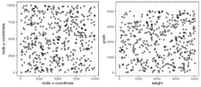
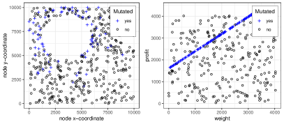
Figure 3. An initial random TTP instance (left plots) and mutation applied to it (explosion mutation to the node coordinates, linear projection mutation to the weight-profit combination; right plots).

EA components

Due to the large number of components of the TTP problem, the EA operators are quite involved. The EA is initialized with a random TTP instance with $n$ nodes and $\mathit{IPN}$ number of items per node. Random in this context means that $n$ points are placed uniformly at random in the Euclidean sub-plane $[0,10\,000]^{2}$ to account for the TSP-component. Moreover, the renting rate $R$ is chosen uniformly at random from the real-valued interval $[0,1\,000]$ to allow for the influence of the travel time on the overall objective score to vary from small to large; this interval’s upper bound is the result of considering the maximum value of $R$ across already known TTP instances and then increasing it further to allow for a broader range of interdependence. Item weights are sampled from $[0,4\,040]$ and profits are sampled from $[0,4\,400]$. Lastly, and in line with (Polyakovskiy et al., 2014), the initial knapsack capacity is $W=\lceil(D/11)\cdot\sum_{m}w_{m}\rceil$ with $D$ chosen uniformly at random from $[1,\ldots,10]$, and the minimum and maximum speeds are kept constant at $v_{min}=0.1$ and $v_{max}=1$.

We build upon work in the context of instance generation for the TSP and adopt mutation operators introduced in (Bossek et al., 2019). The authors proposed a set of mutation operators that aim for rather extreme changes to the node coordinates. This was motivated by the fact that earlier work in the context of evolutionary-guided TSP instance generation, using just small local changes to node coordinates, used to produce instances that in fact showed the aimed strong performance difference, but did not differ much from random uniform instances in terms of visual structure and instance characteristics. One illustrative example for the “creative” mutation operators is the explosion mutation where a center of explosion $c$ and an explosion radius $r>0$ are sampled and all points within Euclidean distance at most $r$ from $c$ are moved away from the explosion center. For an exhaustive description of all operators we refer the interested reader to (Bossek et al., 2019). Note that weights and profits $(w_{i},p_{i}),1\leq i\leq m$ can be interpreted as a point cloud, too. Therefore, we apply the same operators to these values. Figure 3 illustrates an exemplary initial TTP instance and a mutant based on two different mutation operators. Here, the rather disruptive nature of the mutation operators becomes obvious. We apply Gaussian mutation to the renting rate $R$, i.e., we add a random number stemming from a normal distribution with mean value zero and standard deviation 10 to it. Mutation of the knapsack capacity $W$ follows its random initialization scheme discussed above and is thus more disruptive. All variation operations are finalized with a repair step (random re-positioning within the bounds) that ensures that the respective coordinates/points/parameters stay within their initially defined bounds (see initialization). In each iteration, the EA chooses one out of 10 mutation operators with equal probability to generate a mutant where all components are subject to mutation in every iteration.

Further parameters

We consider $n=200$ nodes and $\mathit{IPN}\in\{1,3,5,10\}$ items per node. With respect to the proposed fitness functions we generate for each combination of $n$, $\mathit{IPN}$ and fitness function approach $240$ instances: for the two fitness functions where rankings actually matter, the set contains each 10 instances for each of the 24 $(n,\mathit{IPN},\text{ranking})$-combinations. In total the generated benchmark set contains $N=720$ instances. Within the fitness function evaluation each relevant heuristic is run $k=5$ times independently with a time-limit of $10$ seconds per run. The performance of an algorithm is defined as the unique median over all $k$ runs. Each run of the evolving EA is given a wall-time of 48 hours as the single termination criterion: the EA terminates after $\approx 47$ hours and the last hour is used to run each of the three TTP heuristics 30 times independently on the evolved TTP instance for final evaluation. All experiments were run on the High-Performance-Cluster ¡anonymous¿. We implemented the EA in the statistical programming language R (R Core Team, 2020) in version 4.0.0; for the TTP heuristics we rely on existing Java implementations kindly provided by the original authors of (Faulkner et al., 2015). All scripts and data are made available in a public GitHub.

7. Discussion of results

We now discuss observations based on detailed data analysis of the generated instance set. Saying it right away: the results in the considered TTP setting are less pleasing than expected and may thus partially be considered as negative results. However, we have plausible explanations for these artifacts and feel like the lessons learned in the course of preparing this manuscript are of high scientific interest for researchers in the field.

7.1. Desired versus actual rankings

We first consider the results for the fitness function pairwise and explicit-ranking where the ranking is a parameter of the fitness function. Figure 4 shows the rate of “successful” jobs for each ranking for the pairwise and explicit-ranking setting. Successful in this context means that the final evaluations reflect the desired ranking used by the fitness function. We observe a clear trend. In the pairwise-setting (right plot in Figure 4) the EA succeeds in $85\%$ and even $97.5\%$ of the cases in generating instances where C2 performs better than S4 and S2 respectively. All other cases are far less successful. In particular, it seems difficult to evolve instances where S2 or S4 outperform C2 (success rates of $10\%$ and $20\%$ respectively). This observation indicates that C2 is clearly dominating the algorithm portfolio and can be attributed to the more sophisticated working principles of C2 in direct comparison to S2 and S4. Looking at the left plot in Figure 4 we see that this issue directly transfers to the success rate of jobs guided by the explicit-ranking fitness function. This is plausible: if S2 $>$ C2 is hardly possible, we cannot expect S2 $>$ C2 $>$ S4 to be any easier.

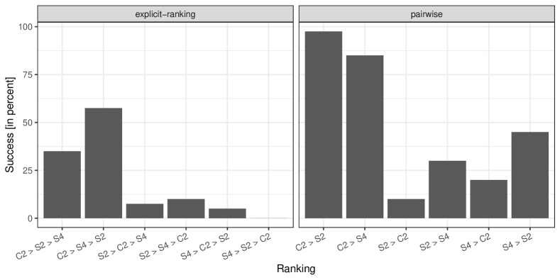
Figure 4. Percentage of successful evolving jobs, i.e., jobs where the median of the final 30 evaluations in fact reflects the ranking that was aimed for.

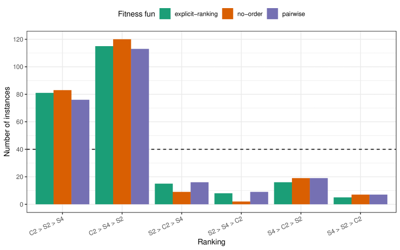
Figure 5. Number of instances evolved for each ranking split by fitness-function. The dashed line indicates the number of instances that the experimental setup aimed for for each ranking.

Figure 5 shows a different perspective. Here, the ranking on the $x$-axis is the actual ranking based on the final evaluations after the evolving process completed. This allows to integrate the results for the third fitness function, no-order, into the plot. The plot reveals that most evolved instances are easiest for C2 with each more than 110 instances in total showing the ranking C2 $>$ S4 $>$ S2 and about 80 instances reflecting C2 $>$ S2 $>$ S4. Instances where algorithms S2/S4 score first place are rather scarce (far less than the anticipated 40 instances for each ranking). Note however, that at least for S2 the results for the pairwise and explicit-ranking are superior to the plain no-order setting.

7.2. Investigating issues

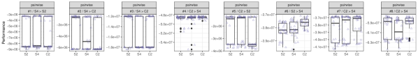
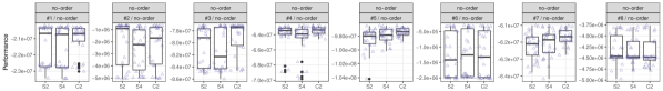
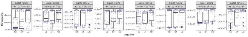
Figure 6. Distribution of performance values for each eight instances evolved by fitness function pairwise (top row), no-order (middle row) and explicit-ranking (bottom row).

We now take a closer look at the performance of the algorithms on a representative subset of the evolved instances. Figure 6 shows boxplots of the performance of all three algorithms (each 30 runs) on eight representative evolved instances for each of the three fitness functions: pairwise, no-order and explicit ranking from top to bottom. We can identify two repeating patterns that pose difficulties to the EA; each alone can fool the EA and in particular the combination of both aspects. The first one is due to (roughly) bi-modal behavior of all or a subset of the algorithms. We can observe this, e.g. in the first three plots of the first row, the first plot in the second row and the sixth plot in the third row of (blue triangles indicate the raw performance values). Here, the algorithms seemingly run in either one of two local optima or at least multiple optima with very similar objective scores with roughly equal probability. Recall that the EA works with aggregated median performance values (based on each $k=5$ independent runs) and the fitness value in all cases is a composition of differences of median values. Now, for example assume, that algorithm S2 takes the raw performance values $(10,10,1,1,10)$ on some instance $I$: the median value is 10. For S4 we have $(10,1,1,10,1)$ and the median value is 1. In the pairwise setting for the ranking S2 $>$ S4 the fitness value would be $10-1=9$ and the instance might get accepted as the new incumbent instance in the course of optimization. Let us assume that this incumbent is not replaced anymore in subsequent iterations of the EA and the EA returns $I$. Now, due to the described issue, in the final 30 evaluations, the median difference on $I$ might be exactly the other way around indicating S4 $>$ S2. This is what actually happens very often. The other aspect is a high variance of objective scores intermingled with the fact that there are few cases where one algorithm always outperforms its competitors. In fact, on almost all instances, the best objective scores of the worst algorithm (with respect to median performance) are equal to the best scores of the best algorithm. In combination, both discussed issues have the potential to misguide the EA. In fact, looking a the development of the fitness values over time reveals that all EA-runs make progress “in the right direction”. However, final evaluations in most cases show the vice-versa. One could argue that these issues might by overcome by increasing the number $k$ of runs of each algorithm in the fitness-function evaluation. However, follow-up investigations with $k=30$ did not change the overall picture.

7.3. Properties of evolved instances

Next, we characterise the so-called features of the evolved instances. Useful features describe high-level properties of an instance that are (a) computationally undemanding to calculate (at least in comparison to costly runs of optimization algorithms) and (b) well-suited to distinguish algorithm performance. These features can then ideally be used in the context of automatic per-instance algorithm selection to predict the most likely best-performing algorithm from a portfolio (see (Kerschke et al., 2019b) for a recent survey on algorithm selection).

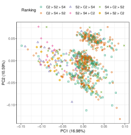
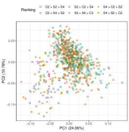
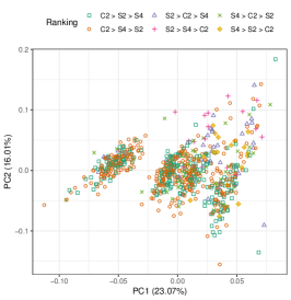
Figure 7. First two principal components results of a principal component analysis on both TSP and KP features (left), only TSP features (center) and only KP features (right).

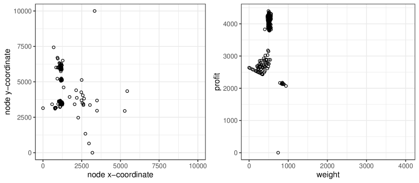
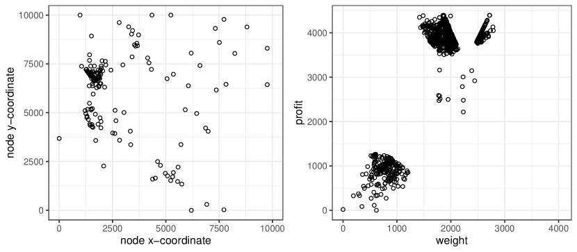
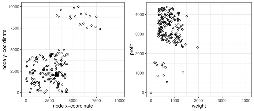
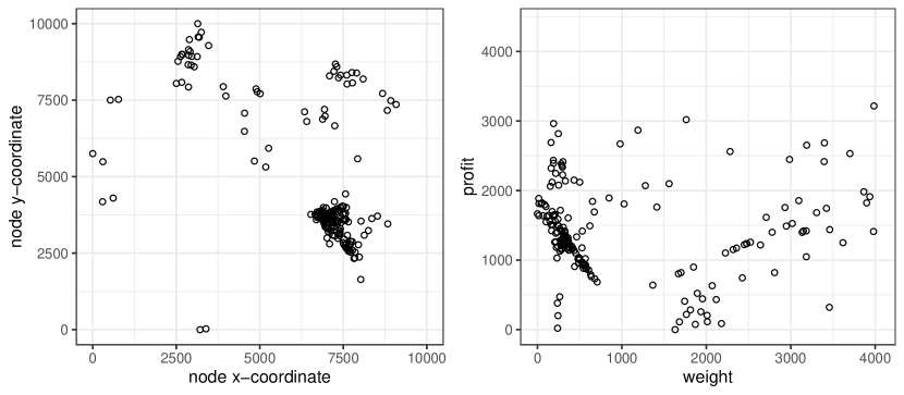
Figure 8. Evolved TTP instances where the desired ranking was achieved successfully for $S2>S4>C2$ (top-left), $S4>C2>S2$ (top right), $C2>S2>S4$ (bottom left) and $C2>S4>S2$ (bottom right).

To the best of our knowledge there is no work on instance characteristics for the TTP besides a brief investigation in the context of algorithm selection (Wagner et al., 2018). Therefore, we treat the TSP and KP components separately. For each instance we calculate a set of features for the TSP taken from the literature. Features involve summary statistics of the edge weights of a minimum spanning tree (e.g., the depth), distance-based features calculated on basis of the distance matrix (mean, median, standard deviation etc.) or properties of the $k$-Nearest-Neighbor Graph (NNG) like the number of weak/strong components it is composed of. In particular the latter $k$-NNG based feature-set proved useful in algorithm selection approaches for the TSP (Pihera and Musliu, 2014). The KP-related weight/profit combination is treated as another TSP and we calculate the same features for the knapsack component of the TSP. This approach results in a set of more than $400$ features in total given. We apply principal component analysis (PCA) to the features and project the instances into the 2-dimensional space spanned by the first two components. Figure 7 shows the 2-dimensional embeddings if PCA was applied with the union of TSP and KP features, TSP features only and KP-features only. The points are colored by their actual ranking based on the final evaluation. Notably, in line with observations made at the beginning of the experimental evaluation, the majority of points represents instances that are easiest for C2 (cf. Figure 5). The total variance in the data explained by the first two principal components (PCs) is not tremendous, but neither is it low. We have $\approx 27.5\%$ in case we use both feature sets, $\approx 34.7$ for TSP-only features and $\approx 39\%$ for KP-only features. In the first and last plot we can identify four (partly overlapping) clusters which can be attributed to the four values $\{1,3,5,10\}$ used for the number of items per node ($\mathit{IPN}$). This makes sense because many of the features are no normalized and thus affected by the number of observations (note that the bounding box for the items is $[0,4\,040]\times[0,4\,400]$ regardless of the choice for $\mathit{IPN}$). Taking a close look at the plots we can see that instances which are easiest for S2 are located in another area of the plot (violet triangles and orange dots) quite well separated from the large clusters where most C2-dominated instances lie.

For example, in the left-most embedding the majority of these instances have a PC1-value below $-0.025$. Making sense of the so-called loadings of the PCA is difficult. There are many features that influence the first and second principal component and it is out of scope of this paper to dive deeper into machine learning models. However, it opens a path for deeper instance-feature analysis and paves the way for a better understanding of TTP-instance hardness. We stress that these observations are particularly nice given the discouraging and unpromising results discussed earlier in this section.

Finally, Figure 8 gives a visual impression of four representative evolved instances. The instances are very diverse owing the disruptive nature of the adopted mutation operators. The overall impression is that S2 works best on instances with rather densely clustered node weights and items, i.e., where there exist subsets of items with similar weights and profits. In contrast, C2 copes better with a wider weight/profit spread.

8. Conclusion and take-away messages

We have studied the task of generating a set of benchmark instances for combinatorial optimization problems by means of evolutionary algorithms. Such a set can aid researchers to get a better understanding of the problem and develop better algorithms. Ideally, such a set is diverse with respect to (1) complementary algorithm performance on a set of algorithms and (2) structural properties of the instances. We aimed for the first goal and targeted the problem of evolving instances where the performance on at least three algorithms follows a given ranking. To this end we proposed fitness functions suited to guide the evolutionary search process in a way that it is balanced with respect to the ranking of solver performance. As part of a proof-of-concept study we adopted our approach to evolve a benchmark set for the Traveling Thief Problem (TTP) and three TTP-heuristics.

The results clearly show that the effectiveness of our approach strongly depends on the algorithm portfolio. As a take-away message we want to make the reader aware of the following potential pitfalls in this branch of research:

1. Unsurprisingly, it is easy to evolve instances that are most reliably solved by the dominating algorithm in the portfolio, but the reverse can be difficult, if not even impossible. Hence, the proposed portfolio necessarily needs to be composed of solvers with strong complementary behavior.

2. The proposed fitness functions can be fooled by certain statistical artifacts of the solver performance. In this work, most notably, severe bi-modality of the performance distribution of single solvers led to a misdirection of the evolutionary search even though the robust median value was used to aggregate over multiple runs.

In future work, we will apply our approach to other optimization problems, and we will improve the algorithm used for the evolution: while a population-based approach will enable us to evolve diverse instances in parallel, we will need to investigate how to evenly distribute them in the space of $N!$ target permutations. For this, established distance measures (see e.g. (Cicirello, 2018)) might prove useful.

Moreover, the formulated take-away messages suggest interesting avenues for further investigations, such as: how do task-specific mutation operator have to be constructed that are better suited to generate instances that are indeed hard for the dominating algorithm; how can alternative summary statistics (e.g., $p$-quantiles) assist to aggregate solver performance?

Acknowledgements. Jakob Bossek acknowledges support by the European Research Center for Information Systems (ERCIS). Markus Wagner acknowledges support by the Australian Research Council projects DP200102364 and DP210102670.

References

- (1)
- Bartz-Beielstein et al. (2020) Thomas Bartz-Beielstein, Carola Doerr, Daan van den Berg, Jakob Bossek, Sowmya Chandrasekaran, Tome Eftimov, Andreas Fischbach, Pascal Kerschke, William La Cava, Manuel Lopez-Ibanez, Katherine M. Malan, Jason H. Moore, Boris Naujoks, Patryk Orzechowski, Vanessa Volz, Markus Wagner, and Thomas Weise. 2020. Benchmarking in Optimization: Best Practice and Open Issues. arXiv:2007.03488 [cs.NE]
- Blank et al. (2017) Julian Blank, Kalyanmoy Deb, and Sanaz Mostaghim. 2017. Solving the Bi-objective Traveling Thief Problem with Multi-objective Evolutionary Algorithms. Springer, 46–60. https://doi.org/10.1007/978-3-319-54157-0_4
- Bonyadi et al. (2013) M. R. Bonyadi, Z. Michalewicz, and L. Barone. 2013. The travelling thief problem: The first step in the transition from theoretical problems to realistic problems. In IEEE Congress on Evolutionary Computation (CEC). 1037–1044. https://doi.org/10.1109/CEC.2013.6557681
- Bonyadi et al. (2014) Mohammad Reza Bonyadi, Zbigniew Michalewicz, Michal Roman Przybylek, and Adam Wierzbicki. 2014. Socially Inspired Algorithms for the TTP. In Genetic and Evolutionary Computation Conference (GECCO). ACM, 421–428. https://doi.org/10.1145/2576768.2598367
- Bonyadi et al. (2019) Mohammad Reza Bonyadi, Zbigniew Michalewicz, Markus Wagner, and Frank Neumann. 2019. Evolutionary Computation for Multicomponent Problems: Opportunities and Future Directions. Springer, 13–30. https://doi.org/10.1007/978-3-030-01641-8_2
- Bossek et al. (2019) Jakob Bossek, Pascal Kerschke, Aneta Neumann, Markus Wagner, Frank Neumann, and Heike Trautmann. 2019. Evolving diverse TSP instances by means of novel and creative mutation operators. In Foundations of Genetic Algorithms (FOGA). ACM, 58–71. https://doi.org/10.1145/3299904.3340307
- Bossek and Trautmann (2016a) Jakob Bossek and Heike Trautmann. 2016a. Evolving Instances for Maximizing Performance Differences of State-of-the-Art Inexact TSP Solvers. In Learning and Intelligent Optimization (LION) (Lecture Notes in Computer Science, Vol. 10079). Springer, 48–59. https://doi.org/10.1007/978-3-319-50349-3_4
- Bossek and Trautmann (2016b) Jakob Bossek and Heike Trautmann. 2016b. Understanding characteristics of evolved instances for state-of-the-art inexact TSP solvers with maximum performance difference. In AI*IA 2016 Advances in Artificial Intelligence, Vol. 10037 LNAI. Springer, 3–12. https://doi.org/10.1007/978-3-319-49130-1_1
- Bowly (2013) Simon Bowly. 2013. Evolving Hard Instances for Graph Colouring Problems. (2013). Australian Mathematical Sciences Institute.
- Chagas et al. (2020) Jonatas B. C. Chagas, Julian Blank, Markus Wagner, Marcone J. F. Souza, and Kalyanmoy Deb. 2020. A non-dominated sorting based customized random-key genetic algorithm for the bi-objective traveling thief problem. Journal of Heuristics (2020). https://doi.org/10.1007/s10732-020-09457-7
- Cheng et al. (2016) Bayi Cheng, Yanyan Yang, and Xiaoxuan Hu. 2016. Supply chain scheduling with batching, production and distribution. International Journal of Computer Integrated Manufacturing 29, 3 (2016), 251–262. https://doi.org/10.1080/0951192X.2015.1032354
- Cicirello (2018) Vincent A. Cicirello. 2018. JavaPermutationTools: A Java Library of Permutation Distance Metrics. Journal of Open Source Software 3, 31 (2018), 950. https://doi.org/10.21105/joss.00950
- El Yafrani and Ahiod (2015) Mohamed El Yafrani and Belaïd Ahiod. 2015. Cosolver2B: an efficient local search heuristic for the travelling thief problem. In International Conference of Computer Systems and Applications (AICCSA). IEEE, 1–5. https://doi.org/10.1109/AICCSA.2015.7507099
- El Yafrani and Ahiod (2016) Mohamed El Yafrani and Belaïd Ahiod. 2016. Population-based vs. single-solution heuristics for the travelling thief problem. In Genetic and Evolutionary Computation Conference (GECCO). ACM, 317–324. https://doi.org/10.1145/2908812.2908847
- El Yafrani and Ahiod (2018) Mohamed El Yafrani and Belaïd Ahiod. 2018. Efficiently solving the Traveling Thief Problem using hill climbing and simulated annealing. Information Sciences 432 (2018), 231–244. https://doi.org/10.1016/j.ins.2017.12.011
- Faulkner et al. (2015) Hayden Faulkner, Sergey Polyakovskiy, Tom Schultz, and Markus Wagner. 2015. Approximate approaches to the traveling thief problem. In Genetic and Evolutionary Computation Conference (GECCO). ACM, 385–392. https://doi.org/10.1145/2739480.2754716
- Forster and Bortfeldt (2012) Florian Forster and Andreas Bortfeldt. 2012. A tree search procedure for the container relocation problem. Computers & Operations Research 39, 2 (2012), 299–309. https://doi.org/10.1016/j.cor.2011.04.004
- Gao et al. (2016) Wanru Gao, Samadhi Nallaperuma, and Frank Neumann. 2016. Feature-Based Diversity Optimization for Problem Instance Classification. In Parallel Problem Solving from Nature (PPSN) (Lecture Notes in Computer Science, Vol. 9921). Springer, 869–879. https://doi.org/10.1007/978-3-319-45823-6_81
- Herring et al. (2020) Daniel Herring, Michael Kirley, and Xin Yao. 2020. Dynamic Multi-objective Optimization of the Travelling Thief Problem. arXiv:2002.02636 [cs.NE]
- Hottung et al. (2020) Andre Hottung, Shunji Tanaka, and Kevin Tierney. 2020. Deep learning assisted heuristic tree search for the container pre-marshalling problem. Computers & Operations Research 113 (2020), 104781. https://doi.org/10.1016/j.cor.2019.104781
- Hutter et al. (2007) Frank Hutter, Holger H. Hoos, and Thomas Stützle. 2007. Automatic Algorithm Configuration Based on Local Search. In AAAI Conference on Artificial Intelligence. AAAI Press, 1152–1157. http://www.aaai.org/Library/AAAI/2007/aaai07-183.php
- Iori and Martello (2010) Manuel Iori and Silvano Martello. 2010. Routing problems with loading constraints. Top 18, 1 (2010), 4–27. https://doi.org/10.1007/s11750-010-0144-x
- Jiang et al. (2014) He Jiang, Wencheng Sun, Zhilei Ren, Xiaochen Lai, and Yong Piao. 2014. Evolving Hard and Easy Traveling Salesman Problem Instances: A Multi-objective Approach. In Simulated Evolution and Learning. Springer, 216–227. https://doi.org/10.1007/978-3-319-13563-2_19
- Jin et al. (2015) Bo Jin, Wenbin Zhu, and Andrew Lim. 2015. Solving the container relocation problem by an improved greedy look-ahead heuristic. European Journal of Operational Research 240, 3 (2015), 837–847. https://doi.org/10.1016/j.ejor.2014.07.038
- Julstrom (2009) Bryant A. Julstrom. 2009. Evolving Heuristically Difficult Instances of Combinatorial Problems. In 11th Annual Conference on Genetic and Evolutionary Computation (Montreal, Québec, Canada). ACM, 279–286. https://doi.org/10.1145/1569901.1569941
- Kerschke et al. (2019a) Pascal Kerschke, Holger H. Hoos, Frank Neumann, and Heike Trautmann. 2019a. Automated Algorithm Selection: Survey and Perspectives. Evolutionary Computation 27, 1 (2019), 3–45. https://doi.org/10.1162/evco_a_00242 arXiv:https://doi.org/10.1162/evco_a_00242 PMID: 30475672.
- Kerschke et al. (2019b) Pascal Kerschke, Holger H. Hoos, Frank Neumann, and Heike Trautmann. 2019b. Automated Algorithm Selection: Survey and Perspectives. Evolutionary Computation 27, 1 (2019), 3–45. https://doi.org/10.1162/evco_a_00242
- Klamroth et al. (2017) Kathrin Klamroth, Sanaz Mostaghim, Boris Naujoks, Silvia Poles, Robin Purshouse, Günter Rudolph, Stefan Ruzika, Serpil Sayın, Margaret M. Wiecek, and Xin Yao. 2017. Multiobjective optimization for interwoven systems. Journal of Multi-Criteria Decision Analysis 24, 1-2 (2017), 71–81. https://doi.org/10.1002/mcda.1598
- Lechien et al. (2021) Thibault Lechien, Jorik Jooken, and Patrick De Causmaecker. 2021. Evolving test instances of the Hamiltonian completion problem. arXiv:2011.02291 [cs.AI]
- Maity and Das (2020) Alenrex Maity and Swagatam Das. 2020. Efficient hybrid local search heuristics for solving the travelling thief problem. Applied Soft Computing (2020), 106284. https://doi.org/10.1016/j.asoc.2020.106284
- Martello et al. (1999) Silvano Martello, David Pisinger, and Paolo Toth. 1999. Dynamic Programming and Strong Bounds for the 0-1 Knapsack Problem. Management Science 45, 3 (March 1999), 414–424. https://doi.org/10.1287/mnsc.45.3.414
- Martins et al. (2017) Marcella S. R. Martins, Mohamed El Yafrani, Myriam R. B. S. Delgado, Markus Wagner, Belaïd Ahiod, and Ricardo Lüders. 2017. HSEDA: A Heuristic Selection Approach Based on Estimation of Distribution Algorithm for the Travelling Thief Problem. In Genetic and Evolutionary Computation Conference (GECCO). ACM, 361–368. https://doi.org/10.1145/3071178.3071235
- Mei et al. (2014) Yi Mei, Xiaodong Li, and Xin Yao. 2014. On investigation of interdependence between sub-problems of the TTP. Soft Computing 20, 1 (2014), 157–172. https://doi.org/10.1007/s00500-014-1487-2
- Mersmann et al. (2012) Olaf Mersmann, Bernd Bischl, Jakob Bossek, Heike Trautmann, Markus Wagner, and Frank Neumann. 2012. Local Search and the Traveling Salesman Problem: A Feature-Based Characterization of Problem Hardness. In Learning and Intelligent Optimization (LION). Springer, 115–129.
- Mersmann et al. (2013) Olaf Mersmann, Bernd Bischl, Heike Trautmann, Markus Wagner, Jakob Bossek, and Frank Neumann. 2013. A novel feature-based approach to characterize algorithm performance for the traveling salesperson problem. Ann. Math. Artif. Intell. 69, 2 (2013), 151–182. https://doi.org/10.1007/s10472-013-9341-2
- Muñoz et al. (2018) Mario A. Muñoz, Laura Villanova, Davaatseren Baatar, and Kate Smith-Miles. 2018. Instance spaces for machine learning classification. Machine Learning 107, 1 (2018), 109–147. https://doi.org/10.1007/s10994-017-5629-5
- Muñoz and Smith-Miles (2020) Mario A. Muñoz and Kate Smith-Miles. 2020. Generating New Space-Filling Test Instances for Continuous Black-Box Optimization. Evolutionary Computation 28, 3 (2020), 379–404. https://doi.org/10.1162/evco_a_00262 arXiv:https://doi.org/10.1162/evco_a_00262
- Namazi et al. (2019) Majid Namazi, Conrad Sanderson, M. A. Hakim Newton, and Abdul Sattar. 2019. A Cooperative Coordination Solver for Travelling Thief Problems. arXiv e-print, available at https://arxiv.org/abs/1911.03124.
- Neumann et al. (2018) Aneta Neumann, Wanru Gao, Carola Doerr, Frank Neumann, and Markus Wagner. 2018. Discrepancy-Based Evolutionary Diversity Optimization. In Genetic and Evolutionary Computation Conference (GECCO) (Kyoto, Japan). ACM, 991–998. https://doi.org/10.1145/3205455.3205532
- Neumann et al. (2019a) Aneta Neumann, Wanru Gao, Markus Wagner, and Frank Neumann. 2019a. Evolutionary Diversity Optimization Using Multi-Objective Indicators. In Genetic and Evolutionary Computation Conference (GECCO) (Prague, Czech Republic). ACM, 837–845. https://doi.org/10.1145/3321707.3321796
- Neumann et al. (2019b) Frank Neumann, Sergey Polyakovskiy, Martin Skutella, Leen Stougie, and Junhua Wu. 2019b. A Fully Polynomial Time Approximation Scheme for Packing While Traveling. In Algorithmic Aspects of Cloud Computing. Springer, 59–72. https://doi.org/10.1007/978-3-030-19759-9_5
- Pihera and Musliu (2014) Josef Pihera and Nysret Musliu. 2014. Application of Machine Learning to Algorithm Selection for TSP. In Proceedings of the IEEE 26th International Conference on Tools with Artificial Intelligence (ICTAI). IEEE press, Washington, DC, USA, 47–54. https://doi.org/10.1109/ICTAI.2014.18
- Plata-González et al. (2019) Luis Fernando Plata-González, Ivan Amaya, JoséCarlos Ortiz-Bayliss, Santiago Enrique Conant-Pablos, Hugo Terashima-Marín, and Carlos A. Coello Coello. 2019. Evolutionary-based tailoring of synthetic instances for the Knapsack problem. Soft Computing 23, 23 (2019), 12711–12728. https://doi.org/10.1007/s00500-019-03822-w
- Pollaris et al. (2015) Hanne Pollaris, Kris Braekers, An Caris, Gerrit K Janssens, and Sabine Limbourg. 2015. Vehicle routing problems with loading constraints: state-of-the-art and future directions. OR Spectrum 37, 2 (2015), 297–330. https://doi.org/10.1007/s00291-014-0386-3
- Polyakovskiy et al. (2014) Sergey Polyakovskiy, Mohammad Reza Bonyadi, Markus Wagner, Zbigniew Michalewicz, and Frank Neumann. 2014. A Comprehensive Benchmark Set and Heuristics for the Traveling Thief Problem. In Genetic and Evolutionary Computation Conference (GECCO). ACM, 477–484. https://doi.org/10.1145/2576768.2598249
- R Core Team (2020) R Core Team. 2020. R: A Language and Environment for Statistical Computing. R Foundation for Statistical Computing, Vienna, Austria. https://www.R-project.org/
- Sachdeva et al. (2020) Ragav Sachdeva, Frank Neumann, and Markus Wagner. 2020. The Dynamic Travelling Thief Problem: Benchmarks and Performance of Evolutionary Algorithms. arXiv:2004.12045 [cs.NE]
- Smith-Miles and van Hemert (2011) Kate Smith-Miles and Jano I. van Hemert. 2011. Discovering the suitability of optimisation algorithms by learning from evolved instances. Annals of Mathematics and Artificial Intelligence 61, 2 (2011), 87–104. https://doi.org/10.1007/s10472-011-9230-5
- van Hemert (2003) J. I. van Hemert. 2003. Evolving binary constraint satisfaction problem instances that are difficult to solve. In IEEE Congress on Evolutionary Computation (CEC), Vol. 2. 1267–1273 Vol.2. https://doi.org/10.1109/CEC.2003.1299814
- van Hemert (2006) Jano I. van Hemert. 2006. Evolving Combinatorial Problem Instances That Are Difficult to Solve. Evolutionary Computation 14, 4 (2006), 433–462. https://doi.org/10.1162/evco.2006.14.4.433
- Wagner (2016) Markus Wagner. 2016. Stealing Items More Efficiently with Ants: A Swarm Intelligence Approach to the Travelling Thief Problem. In Swarm Intelligence. Springer, 273–281. https://doi.org/10.1007/978-3-319-44427-7_25
- Wagner et al. (2018) Markus Wagner, Marius Lindauer, Mustafa Mısır, Samadhi Nallaperuma, and Frank Hutter. 2018. A case study of algorithm selection for the traveling thief problem. Journal of Heuristics 24, 3 (2018), 295–320. https://doi.org/10.1007/s10732-017-9328-y
- Wang (2020) Gang Wang. 2020. Integrated Supply Chain Scheduling of Procurement, Production, and Distribution under Spillover Effects. Computers & Operations Research (2020), 1–14. https://doi.org/10.1016/j.cor.2020.105105
- Wu et al. (2018) Junhua Wu, Sergey Polyakovskiy, Markus Wagner, and Frank Neumann. 2018. Evolutionary computation plus dynamic programming for the bi-objective travelling thief problem. In Genetic and Evolutionary Computation Conference (GECCO). ACM, 777–784. https://doi.org/10.1145/3205455.3205488
- Wu et al. (2017) Junhua Wu, Markus Wagner, Sergey Polyakovskiy, and Frank Neumann. 2017. Exact Approaches for the Travelling Thief Problem. In Simulated Evolution and Learning. Springer, 110–121. https://doi.org/10.1007/978-3-319-68759-9_10
- Wuijts and Thierens (2019) Rogier Hans Wuijts and Dirk Thierens. 2019. Investigation of the Traveling Thief Problem. In Genetic and Evolutionary Computation Conference (GECCO). ACM, 329–337. https://doi.org/10.1145/3321707.3321766
- Yafrani et al. (2017) Mohamed El Yafrani, Shelvin Chand, Aneta Neumann, Belaïd Ahiod, and Markus Wagner. 2017. Multi-Objectiveness in the Single-Objective Traveling Thief Problem. ACM, 107–108. https://doi.org/10.1145/3067695.3076010
- Yafrani et al. (2018) Mohamed El Yafrani, Marcella S. R. Martins, Mehdi El Krari, Markus Wagner, Myriam R. B. S. Delgado, Belaïd Ahiod, and Ricardo Lüders. 2018. A Fitness Landscape Analysis of the Travelling Thief Problem. In Genetic and Evolutionary Computation Conference (GECCO). ACM, 277–284. https://doi.org/10.1145/3205455.3205537
- Zouari et al. (2019) Wiem Zouari, Ines Alaya, and Moncef Tagina. 2019. A New Hybrid Ant Colony Algorithms for the Traveling Thief Problem. In Genetic and Evolutionary Computation Conference (GECCO) Companion. ACM, 95–96. https://doi.org/10.1145/3319619.3326785