Abstract

We construct the global phase portraits of inflationary dynamics in teleparallel gravity models with a scalar field nonminimally coupled to torsion scalar. The adopted set of variables can clearly distinguish between different asymptotic states as fixed points, including the kinetic and inflationary regimes. The key role in the description of inflation is played by the heteroclinic orbits which run from the asymptotic saddle points to the late time attractor point and are approximated by nonminimal slow roll conditions. To seek the asymptotic fixed points we outline a heuristic method in terms of the “effective potential” and “effective mass”, which can be applied for any nonminimally coupled theories. As particular examples we study positive quadratic nonminimal couplings with quadratic and quartic potentials, and note how the portraits differ qualitatively from the known scalar-curvature counterparts. For quadratic models inflation can only occur at small nonminimal coupling to torsion, as for larger coupling the asymptotic de Sitter saddle point disappears from the physical phase space. Teleparallel models with quartic potentials are not viable for inflation at all, since for small nonminimal coupling the asymptotic saddle point exhibits weaker than exponential expansion, and for larger coupling disappears too.

x x x Date: 27 May 2021 Global Portraits of Nonminimal Teleparallel Inflation Laur Järv ¹ and Joosep Lember ¹ Laur Järv, Joosep Lember Correspondence: laur.jarv@ut.ee

1 Introduction

While early introductions of a nonminimal coupling between the scalar field and curvature were motivated by e.g. Mach’s principle Brans and Dicke (1961) or conformal invariance Chernikov and Tagirov (1968), the nonminimal coupling appears naturally as a result of quantum corrections to the scalar field on curved spacetime Birrell and Davies (1984) as well as in the effective actions of higher dimensional constructions Overduin and Wesson (1997); Nǎstase (2019). The scalar-tensor framework also offers a convenient representation of many other gravitational theories, like $f(R)$ Clifton et al. (2012); Capozziello and De Laurentis (2011). On the phenomenological side the nonminimal scalars are used to address the dark energy problem of late universe Esposito-Farese and Polarski (2001); Clifton et al. (2012); Bahamonde et al. (2018) as well as the inflationary dynamics of the early universe where nonminimally coupled Higgs Bezrukov and Shaposhnikov (2008) is among the best models to fit observational data Akrami et al. (2020).

Embracing extra freedom in setting the connection allows to present general relativity in alternative geometric formulations Jiménez et al. (2019). By employing teleparallel instead of Riemannian connection the overall curvature vanishes, and by rewriting the Riemann curvature scalar $\accentset{\circ}{R}$ of the Einstein–Hilbert action in terms of the torsion scalar $T$ and a boundary term $B$, $\accentset{\circ}{R}=-T+B$, we obtain the teleparallel equivalent of general relativity Aldrovandi and Pereira (2013); Krssak et al. (2019) where the boundary term does not contribute to the field equations, and the dynamics of gravity is facilitated by torsion alone. Analogously to nonminimal coupling to curvature, it is thus tempting to consider a teleparallel theory where a scalar field is nonminimally coupled to the torsion scalar Geng et al. (2011). So far, no computation has been performed of quantum corrections to the scalar field on a teleparallel background, while imposing the usual Kaluza–Klein metric ansatz on a five-dimensional teleparallel action yields an effective four-dimensional theory where the scalar field is nonminimally coupled to both the torsion scalar and the boundary term Geng et al. (2014a, b), thus effectively to the curvature scalar $\accentset{\circ}{R}$. But purely heuristically it may still make sense to try to couple the scalar field to the part of the action which encodes the gravitational dynamics, and leave aside the boundary part.

In the minimal coupling, a scalar field within teleparallel equivalent of general relativity and a scalar field within general relativity behave exactly the same, but introducing a nonminimal coupling to torsion scalar or Riemannian curvature scalar makes a different theory, like the $f(T)$ theories Ferraro and Fiorini (2007); Bengochea and Ferraro (2009); Linder (2010) differ from their $f(R)$ counterparts. For example, the scalar models nonminimally coupled to $T$ do not enjoy invariance under the basic conformal transformations (rescaling of the metric and reparametrization of the scalar field, but leaving the connection intact) unless one introduces an extra coupling to the $B$-term Yang (2011); Bamba et al. (2013); Wright (2016); Hohmann and Pfeifer (2018). Also, in contrast to the case of a scalar nonminimally coupled to curvature, the parameterized post-Newtonian (PPN) calculation tells that a scalar nonminimally coupled to torsion does not give the effective gravitational constant a Yukawa-type correction and the PPN parameters match those of the minimally coupled scalar field Chen et al. (2015); Mohseni Sadjadi (2017); Emtsova and Hohmann (2020). These features may be attributed to the fact that nonminimal coupling to torsion does not give the scalar field equation a matter source term Järv (2017). It is possible to write the $f(T)$ action in the scalar-torsion form Izumi et al. (2014), but the resulting scalar sees no obvious independent dynamics, thus leaving the issue of the number of degrees of freedom a rather puzzling topic Li et al. (2011); Ferraro and Guzmán (2018a, b, 2020); Blagojević and Nester (2020); Blixt et al. (2020).

Usually teleparallel theories are discussed in the local frame field language where the fundamental variables are tetrad and spin connection components, but a more conventional formulation in terms of the metric and affine connection is also possible Beltrán Jiménez et al. (2018). In either case, in the nonminimal teleparallel context one must make sure the non-Riemannian part of the connection satisfies its own field equations, and it is better to work in the covariant formulation Hohmann et al. (2018), or otherwise the theory would face the embarrassment of lacking local Lorentz invariance (the same applies to $f(T)$ theories Krššák and Saridakis (2016); Golovnev et al. (2017)). Secondly, one should note that imposing a symmetry on the metric does not immediately extend the same symmetry on the teleparallel connection (as it would in the Riemannian case), but the connection must meet its own symmetry conditions Hohmann et al. (2019). For spatially flat Friedmann–Lemaître–Robertson–Walker (FLRW) spacetimes it is not a big issue as a simple ansatz automatically does the job, but already for spatially curved cases the situation turns out to be nontrivial Ferraro and Fiorini (2011); Tamanini and Boehmer (2012); Hohmann et al. (2019); Hohmann (2020).

From the outset, flat FLRW cosmological models with a scalar nonminimally coupled to torsion seem quite promising, as they show basic agreement with observational data Geng et al. (2012), can exhibit phantom-divide crossing (to $\mathrm{\mathrm{w}_{\mathrm{eff}}{}}<-1$) without making the field a phantom Geng et al. (2011); Xu et al. (2012); Jamil et al. (2012); Kucukakca (2013), and can dynamically converge to general relativity in the matter and potential dominated regimes Jarv and Toporensky (2016). The dynamical systems analyses of the theory have been chiefly motivated by addressing the late universe dark energy era and mainly focusing on the exponential potential Wei (2012); Xu et al. (2012); Jamil et al. (2012); Otalora (2013); Bahamonde and Wright (2015); Skugoreva and Toporensky (2016); Mohseni Sadjadi (2015, 2017); D’Agostino and Luongo (2018); Bahamonde et al. (2018); Gonzalez-Espinoza and Otalora (2020); Bahamonde et al. (2021). For power-law potentials the studies indicate that nonminimal torsion coupling leads to a smaller variety of possible dynamical regimes than nonminimal curvature coupling Skugoreva et al. (2015); Skugoreva and Toporensky (2016); Skugoreva (2018). The evolution of cosmological perturbations has been studied in Refs. Geng and Wu (2013); Wu (2016); D’Agostino and Luongo (2018); Abedi et al. (2018); Golovnev and Koivisto (2018); Raatikainen and Rasanen (2019); Gonzalez-Espinoza et al. (2019, 2021), but mostly in a Lorentz noncovariant setting.

The aim of the present paper is to use the methods of dynamical systems Bahamonde et al. (2018) to study the cosmological evolution of scalar field models nonminimally coupled to torsion in spatially flat FLRW backgrounds following the approach of Ref. Järv and Toporensky (2021), and compare the results with models nonminimally coupled to curvature. The adopted variables $(\phi,\tfrac{\dot{\phi}}{H})$ have the benefit of clearly distinguishing all asymptotic states, and we confirm the insight about the central role of heteroclinic orbits in the phase space for the realization of inflation Felder et al. (2002); Urena-Lopez (2012); Alho and Uggla (2015); Alho et al. (2015); Alho and Uggla (2017); Järv and Toporensky (2021) in the torsion case as well. Taking positive quadratic nonminimal couplings with quadratic and quartic potentials as examples, we plot the local and global phase portraits, indicate the leading slow roll trajectory of inflation, and mark the path of the last 50 e-folds of accelerated expansion as well as the range of initial conditions leading to it. We observe how turning on nonminimal coupling to torsion has qualitatively different effects compared to the nonminimal curvature coupling models. The unveiled picture conforms with the asymptotic regimes described in Ref. Skugoreva et al. (2015) and corroborates with the features found earlier in the perturbation analyses, namely that quadratic potential models require very small torsion coupling to be viable Gonzalez-Espinoza et al. (2019), while quartic potentials are problematic in giving successful inflation at all Raatikainen and Rasanen (2019). One should also note that the equations of flat FLRW cosmology with nonminimal coupling to torsion scalar are identical to those with nonminimal coupling to nonmetricity scalar Järv et al. (2018), hence our results pertain also to the models that stem from the yet another alternative geometric formulation of general relativity Beltrán Jiménez et al. (2018); Järv et al. (2018); Jiménez et al. (2019) as well.

The structure of the paper is as follows. In the next Sec. 2 we compare the cosmological equations of a scalar field nonminimally coupled to torsion and curvature, and explain the basic behavior in terms of the “effective mass” and “effective potential.” In Sec. 3 we write the torsion case equations as a dynamical system to prepare for the analyses of Sec. 4 on the quadratic potential and Sec. 5 on the quartic potential case. We offer the concluding comments in Sec. 6.

2 Scalar-curvature vs. scalar-torsion cosmology

2.1 Action and cosmological equations

We can write the action for a scalar field nonminimally coupled to curvature as Esposito-Farese and Polarski (2001); Bezrukov and Shaposhnikov (2008)

$$S=\tfrac{1}{2}\int d^{4}x\sqrt{-g}\left\{-F(\phi)R+\partial_{\mu}\phi\,\partial^{\mu}\phi-2{V}(\phi)\right\}\,$$ (1)

using the natural units where the reduced Planck mass $M_{\mathrm{Pl}}=(8\pi G_{N})^{-1/2}=1$. The nonminimal coupling function $F(\phi)$ makes the effective Planck mass and correspondingly the effective gravitational “constant” dynamical, while we assume $F>0$. We also assume the potential is nowhere negative $V(\phi)\geq 0$, and the scalar is not a ghost,

$$E(\phi)=2F(\phi)+3F_{,\phi}^{2}\geq 0\,.$$ (2)

Here and below the comma denotes a derivative with respect to the scalar field, e.g. $F_{,\phi\phi}=\tfrac{d^{2}F}{d\phi^{2}}$. The condition (2) can be observed as giving the correct sign of the scalar kinetic term in the conformally transformed Einstein frame where the dynamics of the metric and the scalar field are explicitly decoupled Clifton et al. (2012); Capozziello and De Laurentis (2011).

Analogously, the action for a scalar field with nonminimal coupling to torsion is taken to be Geng et al. (2011); Otalora (2013); Hohmann et al. (2018)

$$S=\tfrac{1}{2}\int d^{4}x\sqrt{-g}\left\{F(\phi)T+\partial_{\mu}\phi\,\partial^{\mu}\phi-2{V}(\phi)\right\}\,.$$ (3)

It too exhibits dynamical effective Planck mass and variable gravitational “constant”, hence again it makes sense to assume $F>0$. The situation about ghosts is not immediately obvious, however, since although a conformal transformation of the metric can resolve the $FT$ term in the action, it will not achieve explicit decoupling, since another term arises which couples the scalar to the torsional boundary term Yang (2011); Bamba et al. (2013); Wright (2016); Hohmann and Pfeifer (2018).

In a flat FLRW background,

$$ds^{2}=dt^{2}-a^{2}(t)\,d\mathbf{x}^{2}\,,$$ (4)

the scalar-curvature cosmological equations are in terms of the Hubble function $H=\tfrac{\dot{a}}{a}$ given by Esposito-Farese and Polarski (2001)

$$3FH^{2} = \tfrac{\dot{\phi}^{2}}{2}+V\,\,{-3F_{,\phi}H\dot{\phi}}$$ (5)

$$-2F\dot{H} = \dot{\phi}^{2}\,\,{+F_{,\phi\phi}\dot{\phi}^{2}-F_{,\phi}H\dot{\phi}+F_{,\phi}\ddot{\phi}}$$ (6)

$$\ddot{\phi}+3H\dot{\phi} = -V_{,\phi}\,\,{+3F_{,\phi}(2H^{2}+\dot{H})}\,.$$ (7)

In the scalar-torsion theory one needs to supplement the metric ansatz (4) with the corresponding ansatz on teleparallel connection, which must be endowed with vanishing curvature, obey the same symmetry of spatial homogeneity and isotropy as the metric Hohmann et al. (2019), and also satisfy its own antisymmetric field equations Hohmann et al. (2018). Fortunately in the present case of Cartesian coordinates (4) such connection is easy to find Hohmann et al. (2018, 2019) and the resulting cosmological equations are Geng et al. (2011); Otalora (2013); Hohmann et al. (2018)

$$3FH^{2} = \tfrac{\dot{\phi}^{2}}{2}+V$$ (8)

$$-2F\dot{H} = \dot{\phi}^{2}\,\,{+2F_{,\phi}H\dot{\phi}}$$ (9)

$$\ddot{\phi}+3H\dot{\phi} = -V_{,\phi}\,\,{-3F_{,\phi}H^{2}}\,.$$ (10)

Note that in the minimally coupled limit, $F=1$, these two sets of equations (5)–(7) and (8)–(10) are identical as expected, but switching on nonminimal coupling to curvature or torsion introduces differences. Just by looking one gets an impression that among the two, the nonminimal coupling to torsion seems to have less impact, since the Friedmann equation (8) stays the same as in the minimal coupling. Also note that in the scalar field equations (7) and (10) the $H^{2}$ term comes with a different sign, which does affect the existence conditions of a regime where $\phi$ is stable Skugoreva et al. (2015).

The rate of expansion can be conveniently expressed by the effective barotropic index, which for the scalar-curvature case reads

$$\mathrm{w}_{\mathrm{eff}}{} =-1-\frac{2\dot{H}}{3H^{2}}=-1+\frac{2F_{,\phi\phi}\dot{\phi}^{2}-2F_{,\phi}H\dot{\phi}+2F_{,\phi}\ddot{\phi}+2\dot{\phi}^{2}}{\dot{\phi}^{2}-6F_{,\phi}H\dot{\phi}+2V}\,,$$ (11)

while for the scalar-torsion case

$$\mathrm{w}_{\mathrm{eff}}{} =-1-\frac{2\dot{H}}{3H^{2}}=-1+\frac{4F_{,\phi}H\dot{\phi}+2\dot{\phi}^{2}}{\dot{\phi}^{2}+2V}\,.$$ (12)

In the minimally coupled case the barotropic index is bounded by $-1\leq\mathrm{w}_{\mathrm{eff}}{}\leq 1$, but in the nonminimally coupled models it is also possible to encounter superaccelerated ($\mathrm{w}_{\mathrm{eff}}{}<-1$) as well as superstiff ($\mathrm{w}_{\mathrm{eff}}{}>1$) expansion. When the scalar field stops, $\dot{\phi}=0,\ddot{\phi}=0$, we have de Sitter like behavior with $\mathrm{w}_{\mathrm{eff}}{}=-1$, provided $V>0$.

2.2 “Effective potential” and “effective mass”

By manipulating (“debraiding”) the field equations we can remove $\dot{H}$ from the scalar field equation, yielding in the scalar-curvature case

$$\ddot{\phi}=\frac{1}{E}(-2FV_{,\phi}+4F_{,\phi}V)-\frac{\dot{\phi}^{2}}{E}(3F_{,\phi\phi}F_{,\phi}+F_{,\phi})-3\dot{\phi}H\,.$$ (13)

In the last term we could have also replaced $H$ by a cumbersome square root coming from Eq. (5), but let it remain for the moment. In the scalar-torsion case the analogous manipulation gives

$$\ddot{\phi}=\frac{1}{F}(-FV_{,\phi}-F_{,\phi}V)-\frac{\dot{\phi}^{2}}{2F}F_{,\phi}-3\dot{\phi}H\,.$$ (14)

These equations coincide in the minimally coupled limit,

$$\ddot{\phi}=-V_{,\phi}-3\dot{\phi}H\,.$$ (15)

To understand the scalar field dynamics it is instructive to compare these equations with a “mechanical analogue” of a point particle moving in the $x$-dimension and experiencing a force described by the gradient of an external potential $V$, as well as friction proportional to its velocity,

$$\ddot{x}=\frac{1}{m}(-V_{,x})-\dot{x}\,\textrm{(friction)}\,.$$ (16)

The formal similarity allows us to speak of an “effective potential” and “effective mass” of the system, see Table 1 for the expressions. Roughly speaking, the system finds the points of stationarity, i.e. the fixed points, at the extrema of the “effective potential” which correspond to the vanishing of the “effective force”. These points are stable or unstable depending on whether they are located at the local minimum or maximum of the “effective potential”, respectively. The friction term depends on the effective “speed” and does not directly contribute to the existence of fixed points, but it should carry the correct sign to avoid a spontaneous blow-up.

	Effective mass	Effective potential	Fixed point condition	Stability condition
	$m_{\mathrm{eff}}$	$V_{\mathrm{eff}}$
Minimally coupled	$1$	$V$	$\frac{V_{,\phi}}{V}=0$	$\frac{V_{,\phi\phi}}{V}>0$
Scalar-curvature	$\frac{E}{F^{3}}$	$\frac{V}{F^{2}}$	$\frac{1}{m_{\mathrm{eff}}}\frac{V_{\mathrm{eff},\phi}}{V}=0$	$\frac{1}{m_{\mathrm{eff}}}\frac{V_{\mathrm{eff},\phi\phi}}{V}>0$
Scalar-torsion	$F$	$FV$	$\frac{1}{m_{\mathrm{eff}}}\frac{V_{\mathrm{eff},\phi}}{V}=0$	$\frac{1}{m_{\mathrm{eff}}}\frac{V_{\mathrm{eff},\phi\phi}}{V}>0$

Table 1: Mechanical analogue quantities of the scalar field cosmological equation in the case of minimal coupling (15), nonminimal coupling to curvature (13), and nonminimal coupling to torsion (14). The conditions for the fixed points and their stability were deduced in Ref. Dutta et al. (2020) for the scalar-curvature case, and follow from Eqs. (27), (28) in the scalar-torsion case.

The idea of an “effective potential” has been advocated as a useful concept in the nonminimal curvature coupling case Chiba and Yamaguchi (2008); Skugoreva et al. (2014); Järv et al. (2017); Dutta et al. (2020) where it also turns out to be an invariant quantity under conformal transformations Järv et al. (2015) and thus rules the dynamics in a frame independent way. (Curiously, it can be also extended to theories with an additional coupling to a Gauss–Bonnet term Pozdeeva et al. (2019); Vernov and Pozdeeva (2021).) In the torsion coupling case the “effective potential” was introduced in Ref.  Skugoreva and Toporensky (2016) to explain the existence and stability of de Sitter fixed points, and noted how these points correspond to the “balanced solutions” of Ref. Jarv and Toporensky (2016). In particular, the form of the “effective potential” dictates that for the nonminimal couplings $F=1+\xi\phi^{N}$ and power-law potentials $V\sim\phi^{n}$, regular de Sitter fixed points exist only for negative $n$ with $0<-n<N$ Skugoreva and Toporensky (2016). The different functional form of the “effective potential” can also explain the markedly different cosmological behaviors of scalar-curvature and scalar-torsion models Skugoreva and Toporensky (2016).

Here we would like to complement these insights about the “effective potential” by also introducing an “effective mass” of the system, which should not be confused with the mass of the scalar particle in the quantum picture. In the nonminimal coupling case the “effective mass” is not constant but depends on the value of the scalar field. Therefore the fixed points where the dynamics of the scalar field stops do not only occur at the extrema of the “effective potential”, but also when the “effective mass” becomes infinite (in the language of the mechanical analogue, an infinitely massive object can not be moved by a force that is finite or “less” infinite). For instance with the typical nonminimal coupling function $F=1+\xi\phi^{N}$ this could happen at the asymptotics $|\phi|\to\infty$ when the “effective potential” does not have an extremum there, or for $\xi<0$ at a finite value of $\phi$. Indeed, it is a bit counterintuitive, but even asymptotically diverging power-law potentials $V\sim\phi^{n}$ (with $n>1$) can feature an asymptotic fixed point if the respective condition in Table 1 is satisfied. The explicit examples are the $dS_{\infty}$ point in the minimally coupled and $dS_{s}$ in the $\xi<0$ nonminimal scalar-curvature case Dutta et al. (2020). As we will witness below such situation does also occur in the scalar-torsion models.

To realize inflation by a heteroclinic orbit starting from either a regular or asymptotic fixed point in the phase space Felder et al. (2002); Urena-Lopez (2012); Alho and Uggla (2015); Alho et al. (2015); Alho and Uggla (2017); Järv and Toporensky (2021), that point of origin must be a saddle with the eigenvalue corresponding to the outgoing direction having positive real part. This would correspond to a local or asymptotic maximum of the “effective potential”, or more precisely not fulfilling the respective stability condition in Table 1. In principle, the point could be also nonhyperbolic with the real part of the corresponding eigenvalue zero, but in such case the higher corrections must still make the direction repulsive, although one needs to resort to center manifold theory to carry out a precise analysis.

2.3 Slow roll

To ensure sufficient measure of inflationary expansion and generate nearly scale invariant spectrum of perturbations, the system must evolve in a nearly de Sitter like regime, which typically implies a slowly varying regime for the scalar field. The corresponding slow roll conditions can be read off from the Friedmann equation (5) and the scalar field equation (13) in the scalar-curvature case Järv and Toporensky (2021),

$$3FH^{2}\simeq V\,,\qquad 3H\dot{\phi}\simeq-\frac{2F}{E}\left(V_{,\phi}-\frac{2F_{,\phi}V}{F}\right)\,,$$ (17)

and correspondingly from (8), (14) in the teleparallel scalar-torsion case,

$$3FH^{2}\simeq V\,,\qquad 3H\dot{\phi}\simeq-V_{,\phi}-\frac{F_{,\phi}V}{F}\,,$$ (18)

which matching the result of Ref. Gonzalez-Espinoza et al. (2019). Unsurprisingly, in the minimally coupled limit the conditions coincide in the two cases. One may also note in comparison with Eqs. (13) and (14) that the slow roll conditon is satisfied exactly at the fixed points where the scalar dynamics stops.

3 Dynamical system

Let us adopt the following dimensionless variables for the dynamical system Dutta et al. (2020); Järv and Toporensky (2021)

$$\phi\,,\qquad z=\frac{\dot{\phi}}{H}\,$$ (19)

(also used in Refs. Mohseni Sadjadi (2015, 2017)). Since the scalar field $\phi$ remains one of the variables, the dynamical system will close for any function $F(\phi),V(\phi)$. It is useful to measure the expansion of the universe in dimensionless e-folds $N=\ln a$, introducing ${}^{\prime}=\tfrac{d}{dN}=\tfrac{1}{H}\tfrac{d}{dt}$ as the derivative of dimensionless time. In particular, this implies $\phi^{\prime}=z$, and also the number of expansion e-folds along a particular trajectory in the phase space can be calculated easily as

$$N=\int dN=\int Hdt=\int\frac{H}{\dot{\phi}}d\phi=\int\frac{1}{z}d\phi\,.$$ (20)

Here we assume expanding universe, $\dot{H}>0$, and note that $N>0$ for both increasing and decreasing $\phi$, since in the latter case also $z<0$.

In these variables, the scalar-curvature system (5)-(7) was studied in detail in Refs. Dutta et al. (2020); Järv and Toporensky (2021), and we will not repeat the details here. In the scalar-torsion case the system (8)-(10) can be represented as

$$\phi^{\prime} = z$$ (21)

$$z^{\prime} = \frac{1}{2F}\left((z^{2}-6F)(F\frac{V_{,\phi}}{V}+z)+2F_{,\phi}(z^{2}-3F)\right)$$ (22)

Like in the scalar-curvature case the physical phase space is not spanned by all values of $\phi,z$, but assuming $V\geq 0$ is bounded by the Friedmann constraint. In the scalar-torsion case from (8) we get a bound

$$6F-z^{2}\geq 0\,.$$ (23)

A possible way to read this bound is by noting that it is exactly satisfied in the ultimate kinetic regime of the scalar field where the contribution of the potential can be neglected in the Friedmann equation. Analogously, we can express in these variables the scalar-torsion effective barotropic index (12) as

$$\mathrm{w}_{\mathrm{eff}}{}=-1+\frac{z(z+2F_{,\phi})}{3F}$$ (24)

and the slow roll conditions (18) as

$$z=-\frac{FV_{,\phi}+F_{,\phi}V}{V}$$ (25)

The latter traces a curve in the phase space. It is not an exact solution (trajectory) itself, but approximates the leading solution that draws all other solutions in the neighbourhood to run closer and closer to it. Along the slow roll curve the effective barotropic index is

$$\mathrm{w}_{\mathrm{eff}}{}^{\mathrm{sr}}=-1+\frac{FV^{2}_{,\phi}}{3V^{2}}-\frac{F^{2}_{,\phi}}{3F}\,.$$ (26)

The regular fixed points arise at whenever the RHS of Eq. (21), (22) vanish, i.e. at the values $\phi_{*}$ satisfying

$$\left(-\frac{FV_{,\phi}}{V}-F_{,\phi}\right)\Big{|}_{\phi_{*}}=0\,.$$ (27)

It is easy to check that the regular fixed points correspond to de Sitter like evolution ($\mathrm{w}_{\mathrm{eff}}{}=-1$). They can be either attractors (related to the late universe of dark energy) or saddles (possibly leading to inflation), depending on the signs of the real parts of the eigenvalues

$$\lambda=-\frac{3}{2}\pm\frac{3}{2}\sqrt{1-\frac{4(F^{2}V_{,\phi\phi}+FF_{,\phi\phi}V-2F_{,\phi}^{2}V)}{3FV}}$$ (28)

The properties of the fixed points become clear when analyzed in terms of the effective potential, see the discussion around Table 1.

There might be other fixed points at infinity, which are not easily captured by finite analysis. The behavior of the system at $\phi$ infinity can be revealed with the help of Poincaré compactification

$$\phi_{p}=\frac{\phi}{\sqrt{1+\phi^{2}+z^{2}}}\,,\qquad z_{p}=\frac{z}{\sqrt{1+\phi^{2}+z^{2}}}\,.$$ (29)

The inverse relation between the compact variables $\phi_{p},z_{p}$ and the original ones (19) is

$$\phi=\frac{\phi_{p}}{\sqrt{1-\phi_{p}^{2}-z_{p}^{2}}}\,,\qquad z=\frac{z_{p}}{\sqrt{1-\phi_{p}^{2}-z_{p}^{2}}}\,.$$ (30)

By construction the compact variables are bounded, $\phi_{p}^{2}+z_{p}^{2}\leq 1$, and map an infinite phase plane onto a disc with unit radius. We can express the dynamical system along with the fixed points, slow roll curves, and so on in terms these new variables, to get a compact global picture of the full phase space including the asymptotic regions.

4 Quadratic potential

Let us take as the first example

$$F=1+\xi\phi^{2}\,,\qquad V=\frac{m^{2}}{2}\phi^{2}+\Lambda$$ (31)

and consider only $\xi>0$ to avoid the complications of nonminimal coupling becoming zero and possibly negative. Like Ref. Järv and Toporensky (2021) we treat $\Lambda$ as a tiny regularizing parameter, to avoid the dynamical equation (22) from becoming singular at the origin. We compute all quantities with $\Lambda>0$ and then apply the limit $\Lambda\rightarrow 0$ to present the results. Physically the $\Lambda$ term can be interpreted as a cosmological constant which is relevant only for the late universe and is many magnitudes smaller that the energy scale of inflation. Since we are only interested in the early universe dynamics and not in the late oscillations of the scalar field around the global minimum of the potential, we are well justified to do it.

4.1 Finite analysis

For the model (31) the dynamical system (21)–(22) is

$$\phi^{\prime} =z$$ (32)

$$z^{\prime} =\frac{\phi(z^{2}-6)(\phi z+2)+6\xi\phi^{3}(z^{2}-\phi z-6)-24\xi^{2}\phi^{5}}{2\phi^{2}(1+\xi\phi^{2})}\,.$$ (33)

Note that by construction (22) the factor $m$ cancels out from the dynamical system (33). Also note, that due to the symmetry of the model (31) the system (32)–(33) is symmetric under the reflection $(\phi\to-\phi,z\to-z)$. The trajectories of the system are depicted on Figs. 1 and 2, and the phase space exhibits a “diagonal” symmetry.

The barotropic index (24) is

$$\mathrm{w}_{\mathrm{eff}}{} =-1+\frac{z(z+4\xi\phi)}{3(1+\xi\phi^{2})}\,.$$ (34)

On the plots the superaccelerated ($\mathrm{w}_{\mathrm{eff}}{}<-1$) part of the phase space is colored green, while acceleration ($-1\leq\mathrm{w}_{\mathrm{eff}}{}<-\tfrac{1}{3}$) is represented by light green, deceleration ($-\tfrac{1}{3}\leq\mathrm{w}_{\mathrm{eff}}{}\leq 1$) by white, and the expansion rate corresponding to superstiff equation of state ($\mathrm{w}_{\mathrm{eff}}{}>1$) by yellow backgrounds, respectively.

The physical phase space is bounded by (23)

$$z^{2}-6\xi\phi^{2}<6\,.$$ (35)

We see that turning on nonminimal coupling extends the physical phase space towards larger $|z|$ for larger $|\phi|$, and infinite $|z|$ become possible at infinite $|\phi|$. One can check explicitly that the solutions do not cross this boundary, e.g. by computing the scalar product of the flow vector $(\phi^{\prime},z^{\prime})$ and a vector normal to the boundary and seeing it is zero. This also means there is a solution trajectory running along the boundary. On the plots the unphysical regions are covered by grey color.

In the minimally coupled case the layout of the phase space is very simple, as the lines of constant $\mathrm{w}_{\mathrm{eff}}{}$ are horizontal, spanning from $\mathrm{w}_{\mathrm{eff}}{}=-1$ at $z=0$ to the stiff expansion $\mathrm{w}_{\mathrm{eff}}{}=+1$ in the ultimate kinetic regime at the boundary of the physical phase space at $z_{b}^{\pm}=\pm\sqrt{6}$. Nonminimal coupling distorts this straight picture, the boundary does not correspond to a fixed $\mathrm{w}_{\mathrm{eff}}{}$, and superstiff behaviour is also possible near the boundary of the phase space. In particular, tracing the boundary

$$z_{b}^{\pm}(\phi) =\pm\sqrt{6+6\xi\phi^{2}}$$ (36)

where “$+$” corresponds to the upper boundary (maximal value of $z$) and “$-$” to the lower boundary (minimal value of $z$) to the asymptotics $|\phi|\to\infty$ we get the value of the barotropic index as

$$\mathrm{w}_{\mathrm{eff}}{}_{b}^{\pm} =1\pm\sqrt{\frac{32\xi}{3}}$$ (37)

Here $\mathrm{w}_{\mathrm{eff}}{}_{b}^{-}$ corresponds to “upper left” $(-\infty,z_{b}^{+})$ and “lower right” $(\infty,z_{b}^{-})$ boundary asymptotic, and drops from the value $+1$ of minimal coupling ($\xi=0$) to $-\infty$ for infinite coupling ($\xi\rightarrow\infty$). Analogously, $\mathrm{w}_{\mathrm{eff}}{}_{b}^{+}$ corresponds to “upper right” $(\infty,z_{b}^{+})$ and “lower left” $(-\infty,z_{b}^{-})$ boundary asymptotic, it increases from the value $+1$ of minimal coupling to infinite value for inifinite coupling.

The slow roll curve (25) is given by

$$z =-4\phi\xi-\frac{2}{\phi}\,$$ (38)

and is plotted with a dashed black line on the plots. On Fig. 1 left column we can observe how it approximates quite well the leading solution (drawn in orange) which attracts the neighbouring solutions. Like in the scalar-curvature case Järv and Toporensky (2021), the approximation curve overestimates $|z|$ compared to the actual attractor solution and thus exits the accelerated expansion regime at slightly higher $|\phi|$. Although the trajectories experience accelerated expansion already while getting closer to the slow roll mode, the expansion during this approach amounts to a few e-folds at best. Only in the vicinity of the leading trajectory the evolution of the scalar field is slow enough to generate significant expansion. On the plots the part of the leading trajectory that corresponds to the last 50 e-folds before the end of accelerated expansion is marked by a red highlight.

The set of initial conditions which lead to at least 50 e-folds of expansion are covered by a semi-transparent light red hue on the plots. In the discussions of good initial conditions for inflation it is usually assumed that the energy density of the field is Planckian, since one may expect that the effects of quantum gravity will become significant above this scale and alter the dynamics. However, in the nonminimally coupled theories where the effective Planck mass is field dependent, the assessment becomes more involved. For this reason some authors have preferred to investigate the whole range of good initial conditions also looking beyond the Planckian density as measured in the units of late Universe Mishra et al. (2020). Here we follow the approach of Ref. Järv and Toporensky (2021) where the focus turned form good initial conditions to good trajectories, as a single trajectory can represent a set of possible initial data. Looking at the plot 1 of minimal coupling we see that beyond certain $|\phi|$ almost all trajectories converge to the leading trajectory and experience sufficient inflation, although there are also trajectories at high kinetic regime near the physical boundary of the phase space which approach the leading trajectory too late for completing 50 e-folds. Comparing this with Fig. 1 it becomes apparent that increasing $\xi$ pushes the wide zone of good initial conditions back to large $|\phi|$ and thus reduces the likelihood that random initial conditions could give sufficient inflationary expansion (note that on the plot 1 the units are magnified by $10^{9}$).

For minimal coupling the slow roll curve starts asymptotically at $(\pm\infty,0)$, but even for a tiny nonminimal coupling the asymptotic starting point jumps to infinite $|z|$. For small $\xi$ this in itself is not a grave problem since the physical phase space also extends to infinite $|z|$ at the asymptotics. Moreover, form Eq. (26) we see that in the asymptotic limit $\mathrm{w}_{\mathrm{eff}}{}^{sr}_{|\phi|\to\infty}=-1$, i.e. de Sitter like expansion. However, for $\xi>\tfrac{3}{8}$ the slow roll curve (38) lies entirely in the unphysical region of the phase space, i.e. beyond the bound (36). Although for larger $\xi$ the phase space is still filled by the zones of accelerated expansion, the scalar field evolves there fast and inflation is not realized. For instance Fig. 2 shows how in the case of $\xi=1$ the slow roll curve would occur in the unphysical region instead, marked by a dotted line.

For general $\xi$ there are three regular fixed points, however, for $\xi>0$ there is only one point

$$A: \qquad(0,0)\,.$$ (39)

It is a stable focus and corresponds to the late universe. We can expect more fixed points to reside in the asymptotics, though. Although the potential, effective potential, and their derivatives all diverge as $|\phi|\to\infty$, the fixed point condition listed in Table 1 is still satisfied in the asymptotic limit. We will investigate the issue in the next subsection.

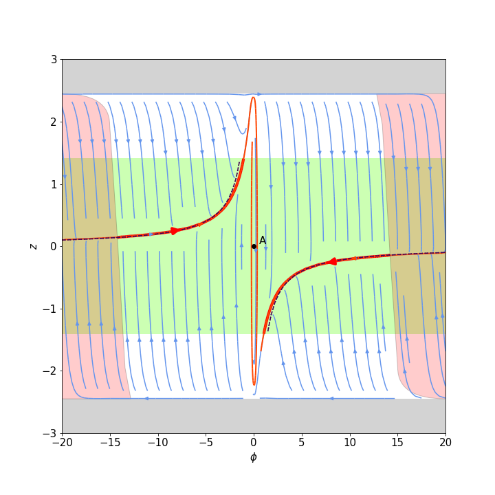
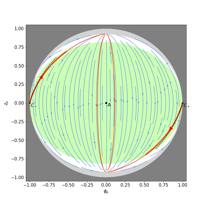
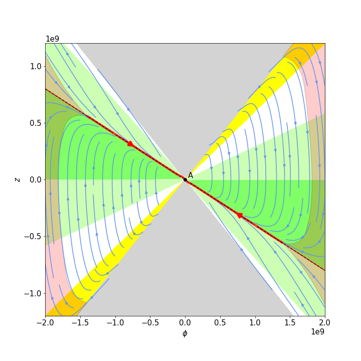
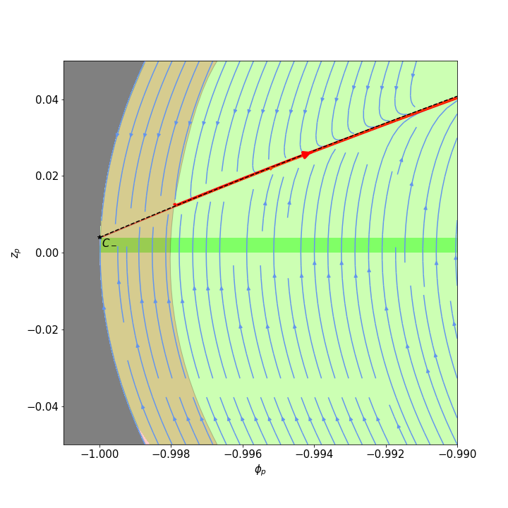
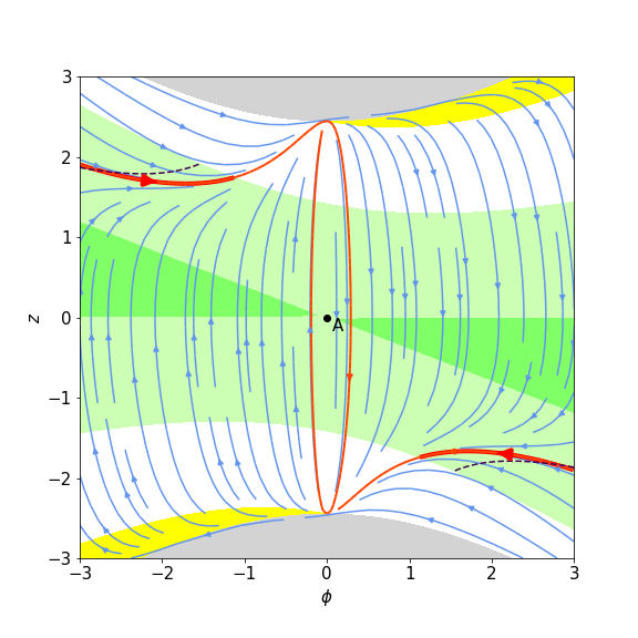
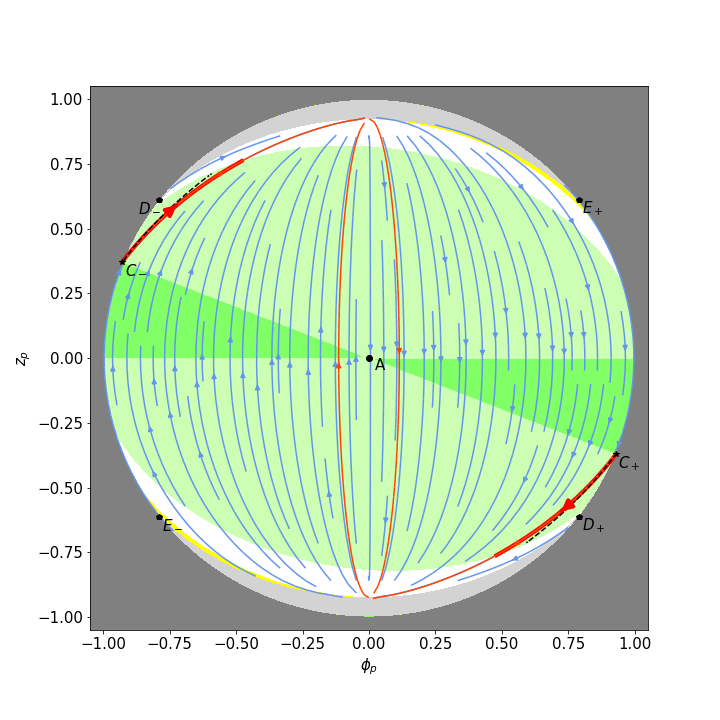
Figure 1: Cosmological dynamics of the quadratic model (31) with $\Lambda=0$, and $\xi=0$ (panels a, b), $\xi=0.001$ (panel d), $\xi=0.1$ (panels c, e, f). Green background stands for superaccelerated, light green accelerated, white decelelerated, and yellow superstiff expansion, while grey covers the unphysical region. Orange trajectories are heteroclinic orbits between the fixed points, wider red part of the master trajectory highlights the 50 last e-folds of inflation, while red semi-transparent cover shows the basin of initial conditions leading to 50 e-folds. The dashed curve marks the path of slow roll approximation.

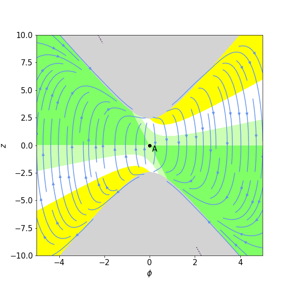
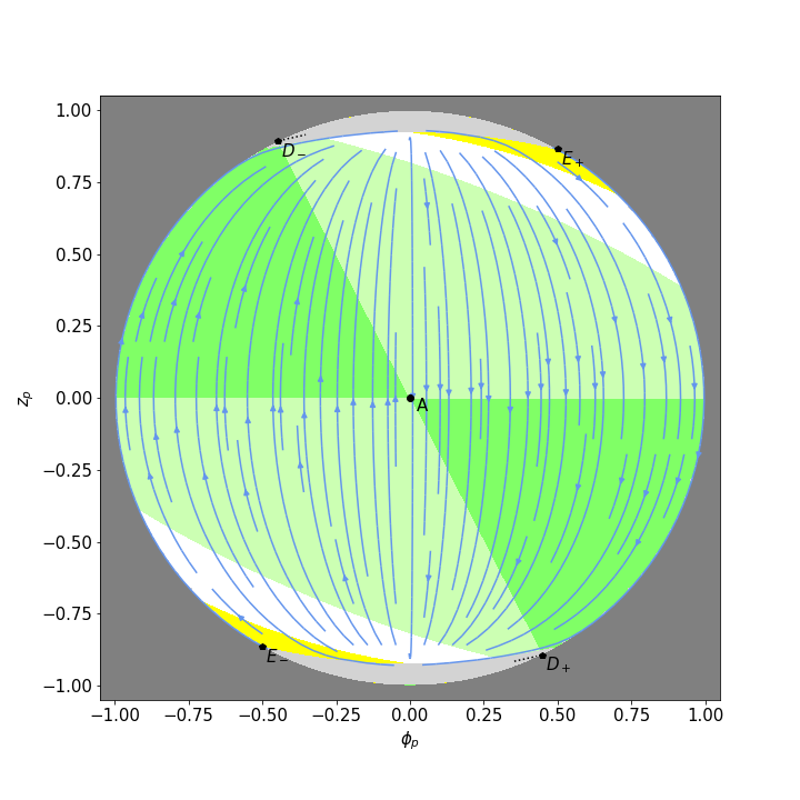
Figure 2: Cosmological dynamics of the quadratic model (31) with $\Lambda=0$, and $\xi=0.5$ (panel b), $\xi=1$ (panel a). Green background stands for superaccelerated, light green accelerated, white decelelerated, and yellow superstiff expansion, while grey covers the unphysical region. Orange trajectories are heteroclinic orbits between the fixed points, wider red part of the master trajectory highlights the 50 last e-folds of inflation, while red semi-transparent cover shows the basin of initial conditions leading to 50 e-folds. The dotted curve marks where the path of the slow roll approximation would be.

4.2 Infinite analysis

In terms of the compact Poincaré variables (29) the system (32), (33) is

$$\phi_{p}^{\prime}= \frac{z_{p}(14q^{2}+6q\phi_{p}z_{p}-\phi_{p}z_{p}^{3})}{2(q+\xi\phi_{p}^{2})}+\frac{\xi\phi_{p}^{2}z_{p}(19q+3\phi_{p}z_{p}-2z_{p}^{2})}{q+\xi\phi_{p}^{2}}+\frac{12\xi^{2}\phi_{p}^{4}z_{p}}{q+\xi\phi_{p}^{2}}$$ (40)

$$z_{p}^{\prime}= -\frac{12q^{3}+12q^{2}\phi_{p}^{2}+6q^{2}\phi_{p}z_{p}-2q^{2}z_{p}^{2}+6q\phi_{p}^{3}z_{p}-q\phi_{p}z_{p}^{3}-\phi_{p}^{3}z_{p}^{3}}{2\phi_{p}(q+\xi\phi_{p}^{2})}$$

$$-\frac{\xi\phi_{p}(18q^{2}+18q\phi_{p}^{2}+3q\phi_{p}z_{p}-3qz_{p}^{2}+3\phi_{p}^{3}z_{p}-2\phi_{p}^{2}z_{p}^{2})}{q+\xi\phi_{p}^{2}}-\frac{12\xi^{2}\phi_{p}^{3}(q+\phi_{p}^{2})}{q+\xi\phi_{p}^{2}}\,.$$ (41)

We have introduced a shorthand notation

$$q=1-\phi_{p}^{2}-z_{p}^{2}\,.$$ (42)

as the asymptotic infinity of the phase space is mapped to $q=0$. The system still retains its “diagonal” symmetry, now manifesting in terms of the compact variables as $(\phi_{p}\to-\phi_{p},z_{p}\to-z_{p})$. In these variables we can also express the effective barotropic index (34) as

$$\mathrm{w}_{\mathrm{eff}}{} =-1+\frac{z_{p}\left(z_{p}+4\xi\phi_{p}\right)}{3\left(q+\xi\phi_{p}^{2}\right)}\,,$$ (43)

the physical phase space domain (35) as

$$\frac{z_{p}^{2}-6\xi\phi_{p}^{2}}{q}<6\,,$$ (44)

and the slow roll curve (38) as

$$\frac{2q+\phi_{p}z_{p}+4\xi\phi_{p}^{2}}{\sqrt{q}\phi_{p}} =0\,.$$ (45)

The final attractor fixed point of the late universe is mapped to the origin,

$$A: \qquad(0,0)\,,$$ (46)

in these variables, and retains its focus character too.

By carefully taking the $q\to 0$ limit in the system (40)–(41) we can detect an asymptotic pair of fixed points

$$C_{\pm}: \qquad(\pm\Omega_{1},\mp\sqrt{1-\Omega_{1}^{2}})\,,$$ (47)

where

$$\Omega_{1} =\frac{1}{\sqrt{1+16\xi^{2}}}\,.$$ (48)

Checking with Eq. (43), these points represent de Sitter like expansions, $\mathrm{w}_{\mathrm{eff}}{}=-1$. One should note that in the nonminimal coupling these points do correspond to a regime where the scalar field evolves, as $z$ is not zero. On the other hand, the evolution of the scalar field must be slow, since the slow roll curve (45) reaches this point in the asymptotic limit. These points perform as saddles, as can be seen most clearly on the plot 1. The heteroclinic orbits from $C_{\pm}$ to $A$ rule the inflationary dynamics, and other trajectories in the phase space are attracted by these leading trajectories. As explained before, if another trajectory manages to get to the vicinity of the heteroclinic orbit at sufficiently high $|\phi|$, it has a chance to experience more than 50 e-folds of accelerated expansion.

In the asymptotics there is also another set of fixed points

$$D_{\pm}: \qquad(\pm\Omega_{2},\mp\sqrt{1-\Omega_{2}^{2}})\,,$$ (49)

$$E_{\pm}: \qquad(\pm\Omega_{2},\pm\sqrt{1-\Omega_{2}^{2}})\,,$$ (50)

where

$$\Omega_{2} =\frac{1}{\sqrt{1+6\xi}}\,.$$ (51)

These points correspond to the locations where the boundary of the physical phase space (44) runs into the asymptotic circle representing infinity. Checking with (43), the effective barotropic index at these points is indeed given by (37), i.e. by $\mathrm{w}_{\mathrm{eff}}{}^{-}_{b}$ at $D_{\pm}$ and by $\mathrm{w}_{\mathrm{eff}}{}^{+}_{b}$ at $E_{\pm}$. As these points reside at the boundary of the physical phase space, they correspond to the utmost kinetic regime of the scalar field, either rolling “down” or “up” its potential. For small $\xi$ the points $D_{\pm}$ act as stable nodes where the trajectories originate, but for large $\xi$ they are saddles. The points $E_{\pm}$ are always saddles. In the limit of minimal coupling, $\xi=0$, the points $D_{\pm}$ and $E_{\pm}$ merge with $C_{\pm}$, giving it a hybrid saddle-node character, as seen on Fig. 1.

By comparing (48) and (51) it becomes now clear why the model yields no inflation for $\xi>\tfrac{3}{8}$. As the points $C_{\pm}$ are the origin of the of the leading inflationary trajectories approximated by the slow troll conditions, increasing $\xi$ shifts these points until they move beyond the points $D_{\pm}$ on the asymptotic circle, whereby they find themselves in the unphysical territory of the phase space. This process can be followed step by step on the Figs. 1, 1, 2. When the points $C_{\pm}$ have left the physical phase space, the inflationary guiding paths from $C_{\pm}$ to $A$ are also gone. For the completeness of description let us mention that while the points $C_{\pm}$ are physical, there are asymptotic heteroclinic orbits running into them from both points $D_{\pm}$ and $E_{\pm}$. When the points $C_{\pm}$ become unphysical, the points $D_{\pm}$ change their character from an unstable node to a saddle, and there is an asymptotic heteroclinic orbit from $E_{\pm}$ to $D_{\pm}$. On the other hand, for any $\xi$ there are heteroclinic orbits running along the boundary of the physical phase space from $D_{\pm}$ to $E_{\mp}$.

It is fascinating that we can identify our asymptotic fixed points with the corresponding regimes uncovered by a study which used completely different set of dynamical variables. Indeed, our points $D_{\pm}$ match the properties and the effective barotropic index of points $Q_{3}$ of Ref. Skugoreva et al. (2015), exhibiting the regime of power-law evolution,

$$a(t) =a_{0}|t-t_{0}|^{\tfrac{1}{3-2\sqrt{6\xi}}}\,,\qquad\phi(t)=\phi_{0}|t-t_{0}|^{-\tfrac{\sqrt{6\xi}}{3-2\sqrt{6\xi}}}$$ (52)

(for $\xi\neq\tfrac{3}{8}$), and turning from an unstable node to a saddle at $\xi>\tfrac{3}{8}$, as the eigenvalues tell. Similarly, our points $C_{\pm}$ match the properties and the effective barotropic index of the points $Q_{4}$ of Ref. Skugoreva et al. (2015), exhibiting the regime of exponential evolution,

$$a(t) =a_{0}e^{\sqrt{\tfrac{m}{2\xi(3-8\xi)}}(t-t_{0})}\,,\qquad\phi(t)=\phi_{0}e^{\sqrt{\tfrac{8m\xi}{(3-8\xi)}}(t-t_{0})}$$ (53)

(for $\xi\neq\tfrac{3}{8}$), and saddle point character, as the eigenvalues tell. The points $Q_{1}$ and $Q_{2}$ found in Ref. Skugoreva et al. (2015) occur for negative nonminimal coupling and inverse power law potentials, and thus do not pertain to our model, while our points $E_{\pm}$ represent a very particular regime and were not found in Ref. Skugoreva et al. (2015).

The global phase portraits are depicted on the right panels of Figs. 1, 2 and in summary tell the following story. For small couplings $\xi<\tfrac{3}{8}$ generic solutions start in the ultimate kinetic dominated regime at the points $D_{\pm}$, but are attracted by the pair of inflationary attractor orbits that originate at the points $C_{\pm}$, initially manifest slow roll, and end up at the attractor point $A$ of the late universe. Solutions which converge to the leading inflationary trajectory soon enough have a chance to enjoy at least 50 e-folds of accelerated expansion. For larger couplings $\xi\geq\tfrac{3}{8}$ the inflationary solution is not present at all. Then the asymptotic fixed points are all saddles and it is hard to pinpoint the origin of generic solutions, which all exhibit fast oscillations, and end at the point $A$ of the late universe. Therefore this picture is roughly consistent with the perturbation analysis of Ref.  Gonzalez-Espinoza et al. (2019), which found that quadratic potential models require very small torsion coupling to be viable.

5 Quartic potential

As the second example, let us take the quartic potential,

$$F=1+\xi\phi^{2}\,,\qquad V=\frac{\lambda}{4}\phi^{4}+\Lambda\,,$$ (54)

and again consider only $\xi>0$ to avoid complications. As before, we will treat $\Lambda$ as a tiny regularizing parameter, applying the limit $\Lambda\to 0$ to present the results.

5.1 Finite analysis

For the model (54) the dynamical system (21)–(22) is

$$\phi^{\prime} =z$$ (55)

$$z^{\prime} =\frac{\phi^{3}(\phi z+4)(z^{2}-6)+2\xi\phi^{5}(4z^{2}-3\phi z-30)-36\xi^{2}\phi^{7}}{2\phi^{4}(1+\xi\phi^{2})}$$ (56)

Again by construction the factor $\lambda$ cancels out from the dynamical system (56). Also, due to the symmetry of the model the system is symmetric under the reflection $(\phi\to-\phi,z\to-z)$, and the phase space exhibits a “diagonal” symmetry on Figs. 3.

The barotropic index (24) is

$$\mathrm{w}_{\mathrm{eff}}{} =-1+\frac{z(z+4\xi\phi)}{3(1+\xi\phi^{2})}$$ (57)

while the respective color coding is the same for superaccelerating, accelerating, usual decelerating and superstiff expansions on Fig. 3. The physical phase space is bounded by (23)

$$z^{2}-6\xi\phi^{2}<6\,,$$ (58)

which coincides with the bound of the quadratic model (35), as it is independent of the potential. Therefore the “upper” and “lower” boundaries of the physical phase space

$$z_{b}^{\pm}(\phi) =\pm\sqrt{6+6\xi\phi^{2}}$$ (59)

as well as the effective barotropic index at the respective boundaries,

$$\mathrm{w}_{\mathrm{eff}}{}_{b}^{\pm} =1\pm\sqrt{\frac{32\xi}{3}}$$ (60)

are exactly the same. Recall that the boundary represents the ultimate kinetic regime of the scalar field, where the effect of the potential can be neglected.

The slow roll curve (25) is given by

$$z =-6\phi\xi-\frac{4}{\phi}$$ (61)

and plotted again with a dashed black line on the plots. On Figs. 3, 3 we can observe how it approximates the leading solutions (drawn in orange) which attract the neighbouring solutions. Along the leading trajectory and around its immediate vicinity the evolution of the scalar field is the slowest and offers the best conditions for sustained accelerated expansion. However, only for the minimal coupling and really tiny nonminimal coupling we can have at least 50 e-folds of accelerated expansion, marked by a red highlight on the leading trajectory. As before, the set of initial conditions which lead to at least 50 e-folds of expansion are covered by a semi-transparent light red hue on the plots.

For minimal coupling the slow roll curve starts asymptotically at $(\pm\infty,0)$, while after turning on the nonminimal coupling the asymptotic starting point jumps to infinite $|z|$, like we saw already in the quadratic case. But in contrast to the quadratic case, the effective barotropic index along the slow roll curve does not reach the de Sitter value in the asymptotics, showing only

$$\mathrm{w}_{\mathrm{eff}}{}^{sr}_{|\phi|\to\infty}=-1+4\xi$$ (62)

instead. This explains why it is so hard to get sufficient number of e-folds in accelerated expansion for the nonminimal coupling, as even at the beginning of the slow roll path the expansion rate is not high enough. Further on, for $\xi>\tfrac{1}{6}$ the slow roll curve (61) lies entirely in the unphysical region of the phase space, i.e. beyond the bound (36), a qualitative change much alike to the quadratic case. Although for larger $\xi$ the phase space is still filled by the zones of accelerated and superaccelerated expansion, the scalar field evolves everywhere fast and inflation is not realized. The plot 3 illustrates how for larger $\xi$ there is no leading attractor trajectory or slow roll curve to approximate it, while the solutions are instead pushed close to the boundary of the physical phase space, i.e. into the strongly kinetic regime.

For $\xi>0$ and $\Lambda\to 0$ the system (55)–(56) has only one regular fixed point,

$$A: \qquad(0,0)\,$$ (63)

which is a stable node for $\xi\leq\tfrac{3}{8}$ and a stable focus for $\xi>\tfrac{3}{8}$. But the reasoning around Table. 1 indicates that there should be additional fixed points in the asymptotics, to be revealed in the next subsection.

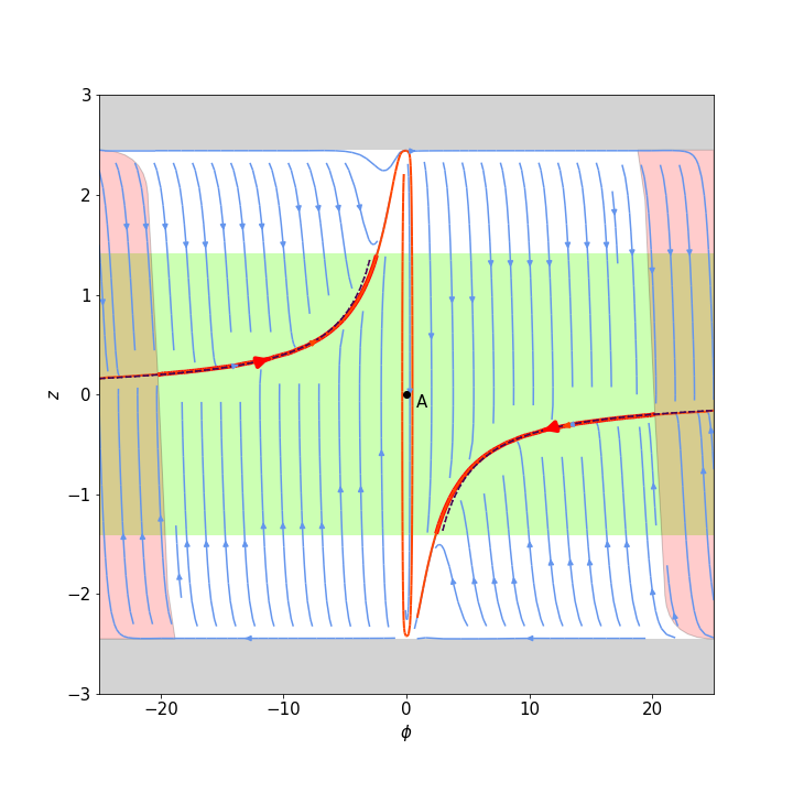
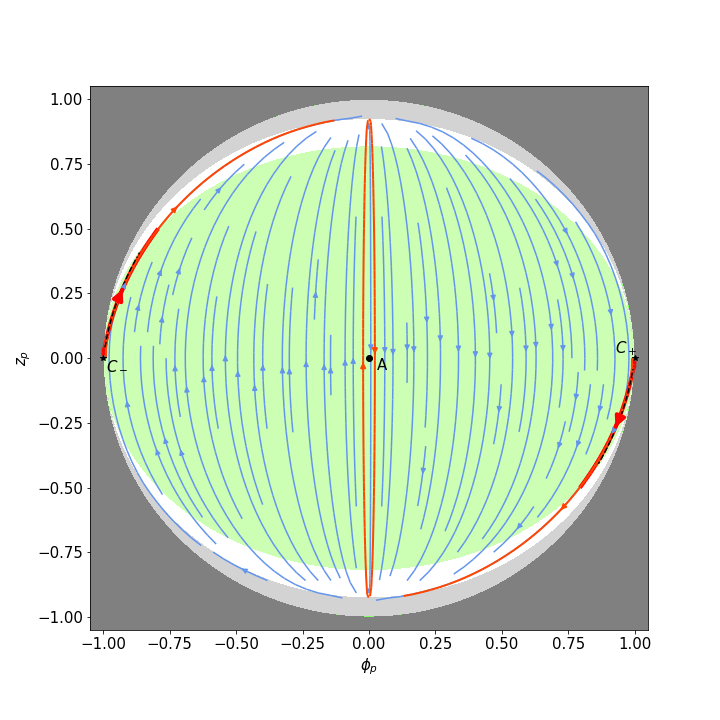
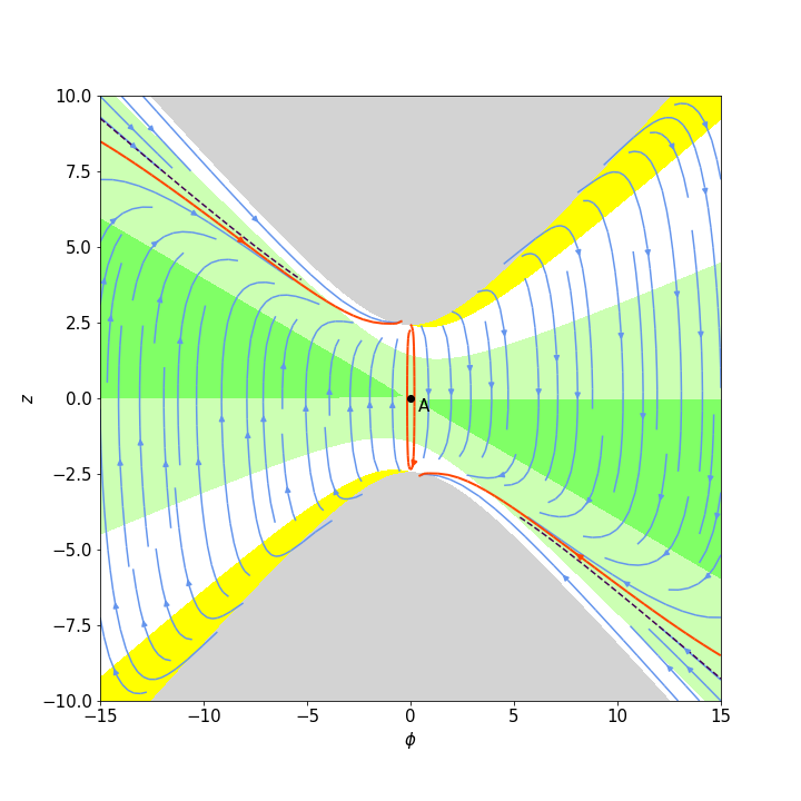
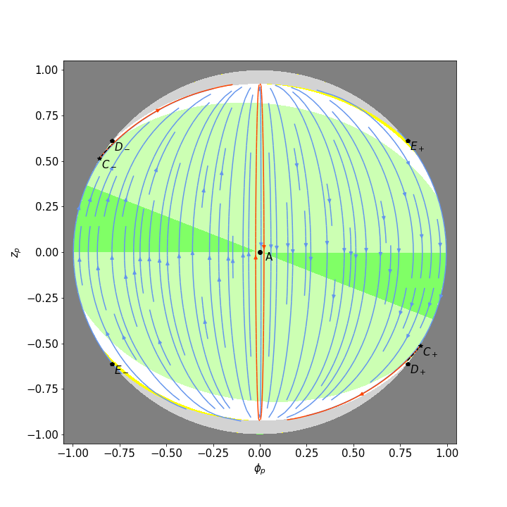
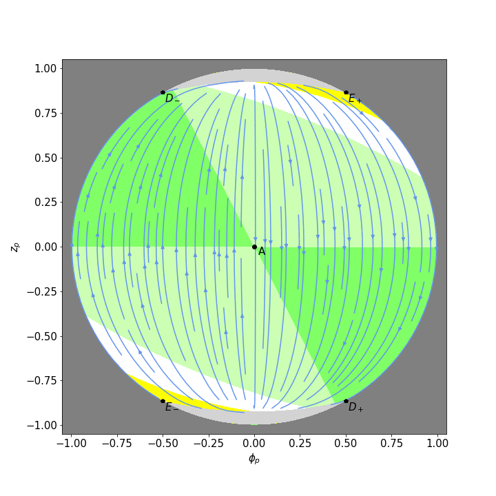
Figure 3: Cosmological dynamics of the quartic model (54) with $\Lambda=0$, and $\xi=0$ (panels a, b), $\xi=0.1$ (panels c, d), $\xi=0.5$ (panel f), $\xi=1$ (panel e). Green background stands for superaccelerated, light green accelerated, white decelelerated, and yellow superstiff expansion, while grey covers the unphysical region. Orange trajectories are heteroclinic orbits between the fixed points, wider red part of the master trajectory highlights the 50 last e-folds of inflation, while red semi-transparent cover shows the basin of initial conditions leading to 50 e-folds. The dashed curve marks the path of slow roll approximation.

5.2 Infinite analysis

In terms of the compact Poincaré variables (29) the system (55), (56) is

$$\phi_{p}^{\prime}= \frac{z_{p}(26q^{2}+6q\phi_{p}z_{p}-2qz_{p}^{2}-\phi_{p}z_{p}^{3})}{2(q+\xi\phi_{p}^{2})}+\frac{\xi\phi_{p}^{2}z_{p}(31q+3\phi_{p}z_{p}-3z_{p}^{2})}{q+\xi\phi_{p}^{2}}+\frac{18\xi^{2}\phi_{p}^{4}z_{p}}{q+\xi\phi_{p}^{2}}$$ (64)

$$z_{p}^{\prime}= -\frac{24q^{3}+24q^{2}\phi_{p}^{2}+6q^{2}\phi_{p}z_{p}-4q^{2}z_{p}^{2}+6q\phi_{p}^{3}z_{p}-2q\phi_{p}^{2}z_{p}^{2}-q\phi_{p}z_{p}^{3}-\phi_{p}^{3}z_{p}^{3}}{2\phi_{p}(q+\xi\phi_{p}^{2})}$$

$$-\frac{\xi\phi_{p}(30q^{2}+30q\phi_{p}^{2}+3q\phi_{p}z_{p}-4qz_{p}^{2}+3\phi_{p}^{3}z_{p}-3\phi_{p}^{2}z_{p}^{2})}{q+\xi\phi_{p}^{2}}-\frac{18\xi^{2}\phi_{p}^{3}(q+\phi_{p}^{2})}{q+\xi\phi_{p}^{2}}\,,$$ (65)

where $q$ measures the distance from the circle representing the asymptotics, (42), as before. The system still manifests the “diagonal” symmetry $(\phi_{p}\to-\phi_{p},z_{p}\to-z_{p})$ on the left panels of Fig. 3.

In the compact variables we can express the effective barotropic index (57) as

$$\mathrm{w}_{\mathrm{eff}}{} =-1+\frac{z_{p}\left(z_{p}+4\xi\phi_{p}\right)}{3\left(q+\xi\phi_{p}^{2}\right)}\,,$$ (66)

the physical phase space domain (58) as

$$\frac{z_{p}^{2}-6\xi\phi_{p}^{2}}{q}<6\,,$$ (67)

and the slow roll curve (61) as

$$\frac{4q+\phi_{p}z_{p}+6\xi\phi_{p}^{2}}{\sqrt{q}\phi_{p}} =0\,.$$ (68)

The fixed point representing late universe is mapped to the origin,

$$A: \qquad(0,0)\,,$$ (69)

and retains its characteristics.

By considering the asymptotic $q\to 0$ limit of the system (64)–(5.2) we can find an asymptotic pair of fixed points

$$C_{\pm}: \qquad\left(\pm\Omega_{1},\mp\sqrt{1-\Omega_{1}^{2}}\right)\,,$$ (70)

where

$$\Omega_{1} =\frac{1}{\sqrt{1+36\xi^{2}}}\,.$$ (71)

Evidently, these points reside at the location where the slow roll curve (68) reaches the asymptotics. They exhibit expansion rates given by the effective barotropic index (62) which is weaker than de Sitter. These points are saddles, and stand as the origin of the heteroclinic orbits which attract other trajectories as they flow to the fixed point $A$ of the late universe. For only extremely small nonminimal couplings $\xi$ there is a limited chance for the surrounding trajectories to converge early enough to the vicinity of these orbits to experience at least 50 e-folds of accelerated expansion.

In the asymptotics one can also find another set fixed points,

$$D_{\pm}: \qquad\left(\pm\Omega_{2},\mp\sqrt{1-\Omega_{2}^{2}}\right)\,,$$ (72)

$$E_{\pm}: \qquad\left(\pm\Omega_{2},\pm\sqrt{1-\Omega_{2}^{2}}\right)\,,$$ (73)

where

$$\Omega_{2} =\frac{1}{\sqrt{1+6\xi}}\,.$$ (74)

They are situated at the locations where the boundary of the physical phase space (67) runs into the asymptotic circle. These points function like their counterparts in the quadratic potential case, with the effective barotropic index $\mathrm{w}_{\mathrm{eff}}{}^{-}_{b}$ for $D_{\pm}$ and $\mathrm{w}_{\mathrm{eff}}{}^{+}_{b}$ for $E_{\pm}$ given by Eq. (60).

Also similarly to the quadratic case, the points $C_{\pm}$ exist only for small nonminimal couplings. At $\xi>\tfrac{1}{6}$ the points $C\pm$ have shifted beyond the points $D_{\pm}$ and become unphysical. Correspondingly, the points $D_{\pm}$ are unstable nodes for small nonminimal couplings, but become saddles for $\xi>\tfrac{1}{6}$. The structure of the heteroclinic orbits is the same as in the quadratic case. Incidentally, the critical value $\xi=\tfrac{1}{6}$ corresponds to $\mathrm{w}_{\mathrm{eff}}{}^{sr}_{|\phi|\to\infty}=-\tfrac{1}{3}$, i.e. where the points $C_{\pm}$ lose the property of accelerated expanision.

The fixed points described above match nicely the results of Ref. Skugoreva et al. (2015), where the corresponding regimes we found using a complitely different set of dynamical variables. Our points $D_{\pm}$ can be identified with the points $Q_{3}$, exhibiting the regime of power-law evolution (52). Our points $C_{\pm}$ can be identified with the points $Q_{4}$, which in the quartic case do not exhibit exponential evolution (53), but another power-law regime

$$a(t) =a_{0}|t-t_{0}|^{\tfrac{1}{6\xi}}\,,\qquad\phi(t)=\phi_{0}|t-t_{0}|^{-1}\,.$$ (75)

They are indeed saddles as the eigenvalues tell. Our points $E_{\pm}$ were not detected in the analysis of Ref. Skugoreva et al. (2015). Note that the variables of Ref. Skugoreva et al. (2015) mapped $Q_{3}$ and $Q_{4}$ to the same point on the asymptotic circle, which complicated the reading of the respective phase portrait there. In our variables the points $C_{\pm}$ and $D_{\pm}$ appeared as distinct for general $\xi$, which concurs with the observation made in Ref. Järv and Toporensky (2021) that the the set $(\phi,\tfrac{\dot{\phi}}{H})$ is really useful to disentangle different asymptotic power law regimes, and delivers an easy to interpret diagram.

A sample of global phase portraits of the model are shown on the right panels of Fig. 3. The story is mostly similar to the quadratic case, but with one important difference. For small couplings $\xi<\tfrac{1}{6}$ the generic solutions start in the ultimate kinetic dominated regime at the points $D_{\pm}$, but are attracted by the pair of heteroclinic orbits that originate at the points $C_{\pm}$, may experience slow roll, and end up at the attractor point $A$ of the late universe. Despite the slow roll property, however, the leading solution starts not as an exponential de Sitter, but as a weaker power law. Hence the model is not conductive for proficient inflation even for small nonmininmal coupling. For larger couplings $\xi\geq\tfrac{1}{6}$ the heteroclinic orbit to $A$ is not present at all. Then the asymptotic fixed points are all saddles and it is hard to pinpoint the origin of generic solutions, which all exhibit fast oscillations, and eventually end at the point $A$ of the late universe. Therefore this picture is in rough agreement with the perturbation analysis of Ref. Raatikainen and Rasanen (2019), which found that the nonminimal scalar-torsion Higgs model (dominated by the quartic term in the potential) is unable to produce inflation.

6 Conclusions

In this paper we have followed the dynamical systems analysis approach of Ref. Järv and Toporensky (2021) to study the global behavior of spatially flat FLRW cosmological models with a scalar field nonminimally coupled to torsion in teleparallel setting. Like in the case of nonminimal coupling to curvature, the set of dynamical variables $(\phi,\tfrac{\dot{\phi}}{H}$) offers an easy to interpret picture of global dynamics, and allows to distinguish the different asymptotic regimes as distinct fixed points. We also confirm the key role of heteroclinic orbits, here trajectories from asymptotic saddle fixed points to the final attractor, in the description of inflation. First, these orbits behave as the leading trajectories to which other solutions are attracted to, thus removing the need to fine-tune the initial conditions, as many solutions initially distant in the phase space will soon follow the same path. Second, these solutions trace out the track of slow roll whereby the expansion is nearly de Sitter, thus providing a good venue for generating inflationary phenomenology. Finally, as inflation is described by a trajectory, and not by a fixed point, there is also a graceful exit from the accelerated expansion at a later stretch of that orbit, when it gets close to the final fixed point of late universe. While it is hard to write down the exact analytic form of the inflationary orbit, there is a simple way to extract the correct nonminimal slow roll conditions from the scalar field equations that yield a curve in the phase space which approximates these orbits well until the end of inflation. In a broader perspective, the description of inflation is just one aspect of a more comprehensive endeavor to map out the entire history of universe in terms of fixed points and the heteroclinic orbits connecting them Dutta et al. (2020).

The asymptotic fixed points, from where the inflationary leading trajectory originates, can exhibit de Sitter like expansion ($\mathrm{w}_{\mathrm{eff}}{}=-1$), but do not necessarily correspond to a usual de Sitter solution of constant scalar field. In Sec. 2 we outlined a general heuristic method to detect such fixed points by introducing the concepts of “effective potential” and “effective mass”, inspired by an analogy from mechanics. We point out that the fixed points of the scalar field do not only occur at the extrema of the “effecive potential”, but can be also caused by the “effective mass” becoming infinite. As for scalars nonminimally coupled to curvature and nonminimally coupled to torsion the “effective potential” and “effective mass” have a rather different functional form, the dynamics of these models can be expected to be rather different, even when the actions look almost identical.

As particular examples we considered models of positive quadratic nonminimal coupling with quadratic and quartic potentials. In the scalar-curvature case the quadratic potential model is endowed with a finite regular saddle de Sitter fixed point which for higher nonminimal coupling shifts closer to the late time attractor and the zone of good initial conditions leading to at least 50 e-folds shrinks to a very narrow stretch Järv and Toporensky (2021). In the scalar-torsion case we found an asymptotic de Sitter point which for higher nonminimal coupling disappears from the physical part of the phase space, making inflation impossible then. Thus although in both cases the most favorable conditions for successful inflation are provided by small nonminimal couplings, the phase portraits are qualitatively different. For quartic potentials, the scalar-curvature case possesses an asymptotic de Sitter point which remains put when the nonminimal coupling increases, but the zone of good initial conditions enlarges, covering almost all available phase space for very large nonminimal coupling Järv and Toporensky (2021). On the other hand, in the scalar-torsion case we found that although the asymptotic saddle fixed point satisfies the slow roll conditions and is the origin of the heteroclinic trajectory, the expansion it corresponds to is power law and not de Sitter like, which severely hampers the prospects for inflation. For larger nonminimal coupling this point also shifts into the unphysical territory of the phase space. Thus the scalar-torsion models with quartic potentials are not really suitable for inflation at all.

One may ask how to improve the chances of inflation for the models with scalar fields nonminimally coupled to torsion? An immediate answer would be to try different potentials and coupling functions. With the heuristic tools of the “effective potential” and “effective mass” at hand, it should be possible to engineer models behaving like the best models nonminimal coupling to curvature has offered. As the impetus and implications from fundamental physics to the reasonable form of nonminimal coupling to torsion are still unclear, alternatives to the usual quadratic coupling may be well explored. Of course, there are also proposals for more general scalar-torsion theories including an additional coupling to vector torsion or the boundary term Bamba et al. (2013); Otalora (2015); Bahamonde and Wright (2015); Gecim and Kucukakca (2018), modification of the kinetic term Rezaei Akbarieh and Izadi (2019), analogue of Horndeski gravity Bahamonde et al. (2019), and even more general frameworks Abedi et al. (2018); Hohmann (2018); Bahamonde et al. (2021). The current method of investigation should be suitable for those as well.

Conceptualization, methodology, writing, editing, supervision, funding acquisition, project administration: L.J.; investigation, formal analysis, validation: L.J. and J.L.; visualization: J.L.

This research was funded by the Estonian Research Council through the project PRG356, as well as by the European Regional Development Fund through the Center of Excellence TK133 “The Dark Side of the Universe”.

References

- Brans and Dicke (1961) Brans, C.; Dicke, R.H. Mach’s principle and a relativistic theory of gravitation. Phys. Rev. 1961, 124, 925–935. doi:\changeurlcolorblack10.1103/PhysRev.124.925.
- Chernikov and Tagirov (1968) Chernikov, N.A.; Tagirov, E.A. Quantum theory of scalar fields in de Sitter space-time. Ann. Inst. H. Poincare Phys. Theor. A 1968, 9, 109.
- Birrell and Davies (1984) Birrell, N.D.; Davies, P.C.W. Quantum Fields in Curved Space; Cambridge Monographs on Mathematical Physics, Cambridge Univ. Press: Cambridge, UK, 1984. doi:\changeurlcolorblack10.1017/CBO9780511622632.
- Overduin and Wesson (1997) Overduin, J.M.; Wesson, P.S. Kaluza-Klein gravity. Phys. Rept. 1997, 283, 303–380, [gr-qc/9805018]. doi:\changeurlcolorblack10.1016/S0370-1573(96)00046-4.
- Nǎstase (2019) Nǎstase, H. Cosmology and String Theory; Vol. 197, Fundamental Theories of Physics, Springer, 2019. doi:\changeurlcolorblack10.1007/978-3-030-15077-8.
- Clifton et al. (2012) Clifton, T.; Ferreira, P.G.; Padilla, A.; Skordis, C. Modified Gravity and Cosmology. Phys. Rept. 2012, 513, 1–189, [arXiv:astro-ph.CO/1106.2476]. doi:\changeurlcolorblack10.1016/j.physrep.2012.01.001.
- Capozziello and De Laurentis (2011) Capozziello, S.; De Laurentis, M. Extended Theories of Gravity. Phys. Rept. 2011, 509, 167–321, [arXiv:gr-qc/1108.6266]. doi:\changeurlcolorblack10.1016/j.physrep.2011.09.003.
- Esposito-Farese and Polarski (2001) Esposito-Farese, G.; Polarski, D. Scalar tensor gravity in an accelerating universe. Phys. Rev. 2001, D63, 063504, [arXiv:gr-qc/gr-qc/0009034]. doi:\changeurlcolorblack10.1103/PhysRevD.63.063504.
- Bahamonde et al. (2018) Bahamonde, S.; Böhmer, C.G.; Carloni, S.; Copeland, E.J.; Fang, W.; Tamanini, N. Dynamical systems applied to cosmology: dark energy and modified gravity. Phys. Rept. 2018, 775-777, 1–122, [arXiv:gr-qc/1712.03107]. doi:\changeurlcolorblack10.1016/j.physrep.2018.09.001.
- Bezrukov and Shaposhnikov (2008) Bezrukov, F.L.; Shaposhnikov, M. The Standard Model Higgs boson as the inflaton. Phys. Lett. 2008, B659, 703–706, [arXiv:hep-th/0710.3755]. doi:\changeurlcolorblack10.1016/j.physletb.2007.11.072.
- Akrami et al. (2020) Akrami, Y.; others. Planck 2018 results. X. Constraints on inflation. Astron. Astrophys. 2020, 641, A10, [arXiv:astro-ph.CO/1807.06211]. doi:\changeurlcolorblack10.1051/0004-6361/201833887.
- Jiménez et al. (2019) Jiménez, J.B.; Heisenberg, L.; Koivisto, T.S. The Geometrical Trinity of Gravity. Universe 2019, 5, 173, [arXiv:hep-th/1903.06830]. doi:\changeurlcolorblack10.3390/universe5070173.
- Aldrovandi and Pereira (2013) Aldrovandi, R.; Pereira, J.G. Teleparallel Gravity; Vol. 173, Springer: Dordrecht, 2013. doi:\changeurlcolorblack10.1007/978-94-007-5143-9.
- Krssak et al. (2019) Krssak, M.; van den Hoogen, R.; Pereira, J.; Böhmer, C.; Coley, A. Teleparallel theories of gravity: illuminating a fully invariant approach. Class. Quant. Grav. 2019, 36, 183001, [arXiv:gr-qc/1810.12932]. doi:\changeurlcolorblack10.1088/1361-6382/ab2e1f.
- Geng et al. (2011) Geng, C.Q.; Lee, C.C.; Saridakis, E.N.; Wu, Y.P. “Teleparallel” dark energy. Phys. Lett. B 2011, 704, 384–387, [arXiv:hep-th/1109.1092]. doi:\changeurlcolorblack10.1016/j.physletb.2011.09.082.
- Geng et al. (2014a) Geng, C.Q.; Luo, L.W.; Tseng, H.H. Teleparallel Gravity in Five Dimensional Theories. Class. Quant. Grav. 2014, 31, 185004, [arXiv:hep-th/1403.3161]. doi:\changeurlcolorblack10.1088/0264-9381/31/18/185004.
- Geng et al. (2014b) Geng, C.Q.; Lai, C.; Luo, L.W.; Tseng, H.H. Kaluza–Klein theory for teleparallel gravity. Phys. Lett. B 2014, 737, 248–250, [arXiv:gr-qc/1409.1018]. doi:\changeurlcolorblack10.1016/j.physletb.2014.08.055.
- Ferraro and Fiorini (2007) Ferraro, R.; Fiorini, F. Modified teleparallel gravity: Inflation without inflaton. Phys. Rev. 2007, D75, 084031, [arXiv:gr-qc/gr-qc/0610067]. doi:\changeurlcolorblack10.1103/PhysRevD.75.084031.
- Bengochea and Ferraro (2009) Bengochea, G.R.; Ferraro, R. Dark torsion as the cosmic speed-up. Phys. Rev. 2009, D79, 124019, [arXiv:astro-ph/0812.1205]. doi:\changeurlcolorblack10.1103/PhysRevD.79.124019.
- Linder (2010) Linder, E.V. Einstein’s Other Gravity and the Acceleration of the Universe. Phys. Rev. D 2010, 81, 127301, [arXiv:astro-ph.CO/1005.3039]. [Erratum: Phys.Rev.D 82, 109902 (2010)], doi:\changeurlcolorblack10.1103/PhysRevD.81.127301.
- Yang (2011) Yang, R.J. Conformal transformation in theories. EPL 2011, 93, 60001, [arXiv:gr-qc/1010.1376]. doi:\changeurlcolorblack10.1209/0295-5075/93/60001.
- Bamba et al. (2013) Bamba, K.; Odintsov, S.D.; Sáez-Gómez, D. Conformal symmetry and accelerating cosmology in teleparallel gravity. Phys. Rev. D 2013, 88, 084042, [arXiv:gr-qc/1308.5789]. doi:\changeurlcolorblack10.1103/PhysRevD.88.084042.
- Wright (2016) Wright, M. Conformal transformations in modified teleparallel theories of gravity revisited. Phys. Rev. D 2016, 93, 103002, [arXiv:gr-qc/1602.05764]. doi:\changeurlcolorblack10.1103/PhysRevD.93.103002.
- Hohmann and Pfeifer (2018) Hohmann, M.; Pfeifer, C. Scalar-torsion theories of gravity II: theory. Phys. Rev. D 2018, 98, 064003, [arXiv:gr-qc/1801.06536]. doi:\changeurlcolorblack10.1103/PhysRevD.98.064003.
- Chen et al. (2015) Chen, Z.C.; Wu, Y.; Wei, H. Post-Newtonian Approximation of Teleparallel Gravity Coupled with a Scalar Field. Nucl. Phys. B 2015, 894, 422–438, [arXiv:gr-qc/1410.7715]. doi:\changeurlcolorblack10.1016/j.nuclphysb.2015.03.012.
- Mohseni Sadjadi (2017) Mohseni Sadjadi, H. Parameterized post-Newtonian approximation in a teleparallel model of dark energy with a boundary term. Eur. Phys. J. C 2017, 77, 191, [arXiv:gr-qc/1606.04362]. doi:\changeurlcolorblack10.1140/epjc/s10052-017-4760-6.
- Emtsova and Hohmann (2020) Emtsova, E.D.; Hohmann, M. Post-Newtonian limit of scalar-torsion theories of gravity as analogue to scalar-curvature theories. Phys. Rev. D 2020, 101, 024017, [arXiv:gr-qc/1909.09355]. doi:\changeurlcolorblack10.1103/PhysRevD.101.024017.
- Järv (2017) Järv, L. Effective Gravitational “Constant” in Scalar-(Curvature)Tensor and Scalar-Torsion Gravities. Universe 2017, 3, 37. doi:\changeurlcolorblack10.3390/universe3020037.
- Izumi et al. (2014) Izumi, K.; Gu, J.A.; Ong, Y.C. Acausality and Nonunique Evolution in Generalized Teleparallel Gravity. Phys. Rev. D 2014, 89, 084025, [arXiv:gr-qc/1309.6461]. doi:\changeurlcolorblack10.1103/PhysRevD.89.084025.
- Li et al. (2011) Li, M.; Miao, R.X.; Miao, Y.G. Degrees of freedom of gravity. JHEP 2011, 07, 108, [arXiv:hep-th/1105.5934]. doi:\changeurlcolorblack10.1007/JHEP07(2011)108.
- Ferraro and Guzmán (2018a) Ferraro, R.; Guzmán, M.J. Hamiltonian formalism for f(T) gravity. Phys. Rev. 2018, D97, 104028, [arXiv:gr-qc/1802.02130]. doi:\changeurlcolorblack10.1103/PhysRevD.97.104028.
- Ferraro and Guzmán (2018b) Ferraro, R.; Guzmán, M.J. Quest for the extra degree of freedom in gravity. Phys. Rev. 2018, D98, 124037, [arXiv:gr-qc/1810.07171]. doi:\changeurlcolorblack10.1103/PhysRevD.98.124037.
- Ferraro and Guzmán (2020) Ferraro, R.; Guzmán, M.J. Pseudoinvariance and the extra degree of freedom in f(T) gravity. Phys. Rev. D 2020, 101, 084017, [arXiv:gr-qc/2001.08137]. doi:\changeurlcolorblack10.1103/PhysRevD.101.084017.
- Blagojević and Nester (2020) Blagojević, M.; Nester, J.M. Local symmetries and physical degrees of freedom in gravity: a Dirac Hamiltonian constraint analysis. Phys. Rev. D 2020, 102, 064025, [arXiv:gr-qc/2006.15303]. doi:\changeurlcolorblack10.1103/PhysRevD.102.064025.
- Blixt et al. (2020) Blixt, D.; Guzmán, M.J.; Hohmann, M.; Pfeifer, C. Review of the Hamiltonian analysis in teleparallel gravity 2020. [arXiv:gr-qc/2012.09180].
- Beltrán Jiménez et al. (2018) Beltrán Jiménez, J.; Heisenberg, L.; Koivisto, T.S. Teleparallel Palatini theories. JCAP 2018, 08, 039, [arXiv:gr-qc/1803.10185]. doi:\changeurlcolorblack10.1088/1475-7516/2018/08/039.
- Hohmann et al. (2018) Hohmann, M.; Järv, L.; Ualikhanova, U. Covariant formulation of scalar-torsion gravity. Phys. Rev. 2018, D97, 104011, [arXiv:gr-qc/1801.05786]. doi:\changeurlcolorblack10.1103/PhysRevD.97.104011.
- Krššák and Saridakis (2016) Krššák, M.; Saridakis, E.N. The covariant formulation of f(T) gravity. Class. Quant. Grav. 2016, 33, 115009, [arXiv:gr-qc/1510.08432]. doi:\changeurlcolorblack10.1088/0264-9381/33/11/115009.
- Golovnev et al. (2017) Golovnev, A.; Koivisto, T.; Sandstad, M. On the covariance of teleparallel gravity theories. Class. Quant. Grav. 2017, 34, 145013, [arXiv:gr-qc/1701.06271]. doi:\changeurlcolorblack10.1088/1361-6382/aa7830.
- Hohmann et al. (2019) Hohmann, M.; Järv, L.; Krššák, M.; Pfeifer, C. Modified teleparallel theories of gravity in symmetric spacetimes. Phys. Rev. D 2019, 100, 084002, [arXiv:gr-qc/1901.05472]. doi:\changeurlcolorblack10.1103/PhysRevD.100.084002.
- Ferraro and Fiorini (2011) Ferraro, R.; Fiorini, F. Non trivial frames for f(T) theories of gravity and beyond. Phys. Lett. B 2011, 702, 75–80, [arXiv:gr-qc/1103.0824]. doi:\changeurlcolorblack10.1016/j.physletb.2011.06.049.
- Tamanini and Boehmer (2012) Tamanini, N.; Boehmer, C.G. Good and bad tetrads in f(T) gravity. Phys. Rev. 2012, D86, 044009, [arXiv:gr-qc/1204.4593]. doi:\changeurlcolorblack10.1103/PhysRevD.86.044009.
- Hohmann (2020) Hohmann, M. Complete classification of cosmological teleparallel geometries. 2020, [arXiv:gr-qc/2008.12186].
- Geng et al. (2012) Geng, C.Q.; Lee, C.C.; Saridakis, E.N. Observational Constraints on Teleparallel Dark Energy. JCAP 2012, 01, 002, [arXiv:astro-ph.CO/1110.0913]. doi:\changeurlcolorblack10.1088/1475-7516/2012/01/002.
- Xu et al. (2012) Xu, C.; Saridakis, E.N.; Leon, G. Phase-Space analysis of Teleparallel Dark Energy. JCAP 2012, 07, 005, [arXiv:gr-qc/1202.3781]. doi:\changeurlcolorblack10.1088/1475-7516/2012/07/005.
- Jamil et al. (2012) Jamil, M.; Momeni, D.; Myrzakulov, R. Stability of a non-minimally conformally coupled scalar field in F(T) cosmology. Eur. Phys. J. C 2012, 72, 2075, [arXiv:gr-qc/1208.0025]. doi:\changeurlcolorblack10.1140/epjc/s10052-012-2075-1.
- Kucukakca (2013) Kucukakca, Y. Scalar tensor teleparallel dark gravity via Noether symmetry. Eur. Phys. J. C 2013, 73, 2327, [arXiv:gr-qc/1404.7315]. doi:\changeurlcolorblack10.1140/epjc/s10052-013-2327-8.
- Jarv and Toporensky (2016) Jarv, L.; Toporensky, A. General relativity as an attractor for scalar-torsion cosmology. Phys. Rev. D 2016, 93, 024051, [arXiv:gr-qc/1511.03933]. doi:\changeurlcolorblack10.1103/PhysRevD.93.024051.
- Wei (2012) Wei, H. Dynamics of Teleparallel Dark Energy. Phys. Lett. B 2012, 712, 430–436, [arXiv:gr-qc/1109.6107]. doi:\changeurlcolorblack10.1016/j.physletb.2012.05.006.
- Otalora (2013) Otalora, G. Scaling attractors in interacting teleparallel dark energy. JCAP 2013, 07, 044, [arXiv:gr-qc/1305.0474]. doi:\changeurlcolorblack10.1088/1475-7516/2013/07/044.
- Bahamonde and Wright (2015) Bahamonde, S.; Wright, M. Teleparallel quintessence with a nonminimal coupling to a boundary term. Phys. Rev. D 2015, 92, 084034, [arXiv:gr-qc/1508.06580]. [Erratum: Phys.Rev.D 93, 109901 (2016)], doi:\changeurlcolorblack10.1103/PhysRevD.92.084034.
- Skugoreva and Toporensky (2016) Skugoreva, M.A.; Toporensky, A.V. Asymptotic cosmological regimes in scalar–torsion gravity with a perfect fluid. Eur. Phys. J. C 2016, 76, 340, [arXiv:gr-qc/1605.01989]. doi:\changeurlcolorblack10.1140/epjc/s10052-016-4190-x.
- Mohseni Sadjadi (2015) Mohseni Sadjadi, H. Onset of acceleration in a universe initially filled by dark and baryonic matters in a nonminimally coupled teleparallel model. Phys. Rev. D 2015, 92, 123538, [arXiv:gr-qc/1510.02085]. doi:\changeurlcolorblack10.1103/PhysRevD.92.123538.
- Mohseni Sadjadi (2017) Mohseni Sadjadi, H. Symmetron and de Sitter attractor in a teleparallel model of cosmology. JCAP 2017, 01, 031, [arXiv:gr-qc/1609.04292]. doi:\changeurlcolorblack10.1088/1475-7516/2017/01/031.
- D’Agostino and Luongo (2018) D’Agostino, R.; Luongo, O. Growth of matter perturbations in nonminimal teleparallel dark energy. Phys. Rev. D 2018, 98, 124013, [arXiv:gr-qc/1807.10167]. doi:\changeurlcolorblack10.1103/PhysRevD.98.124013.
- Bahamonde et al. (2018) Bahamonde, S.; Marciu, M.; Rudra, P. Generalised teleparallel quintom dark energy non-minimally coupled with the scalar torsion and a boundary term. JCAP 2018, 04, 056, [arXiv:gr-qc/1802.09155]. doi:\changeurlcolorblack10.1088/1475-7516/2018/04/056.
- Gonzalez-Espinoza and Otalora (2020) Gonzalez-Espinoza, M.; Otalora, G. Cosmological dynamics of dark energy in scalar-torsion gravity 2020. [arXiv:gr-qc/2011.08377].
- Bahamonde et al. (2021) Bahamonde, S.; Marciu, M.; Odintsov, S.D.; Rudra, P. String-inspired Teleparallel cosmology. Nucl. Phys. B 2021, 962, 115238, [arXiv:gr-qc/2003.13434]. doi:\changeurlcolorblack10.1016/j.nuclphysb.2020.115238.
- Skugoreva et al. (2015) Skugoreva, M.A.; Saridakis, E.N.; Toporensky, A.V. Dynamical features of scalar-torsion theories. Phys. Rev. D 2015, 91, 044023, [arXiv:gr-qc/1412.1502]. doi:\changeurlcolorblack10.1103/PhysRevD.91.044023.
- Skugoreva (2018) Skugoreva, M.A. Late-time power-law stages of cosmological evolution in teleparallel gravity with nonminimal coupling. Grav. Cosmol. 2018, 24, 103–111, [arXiv:gr-qc/1704.06617]. doi:\changeurlcolorblack10.1134/S0202289318010139.
- Geng and Wu (2013) Geng, C.Q.; Wu, Y.P. Density Perturbation Growth in Teleparallel Cosmology. JCAP 2013, 04, 033, [arXiv:astro-ph.CO/1212.6214]. doi:\changeurlcolorblack10.1088/1475-7516/2013/04/033.
- Wu (2016) Wu, Y.P. Inflation with teleparallelism: Can torsion generate primordial fluctuations without local Lorentz symmetry? Phys. Lett. B 2016, 762, 157–161, [arXiv:gr-qc/1609.04959]. doi:\changeurlcolorblack10.1016/j.physletb.2016.09.025.
- Abedi et al. (2018) Abedi, H.; Capozziello, S.; D’Agostino, R.; Luongo, O. Effective gravitational coupling in modified teleparallel theories. Phys. Rev. D 2018, 97, 084008, [arXiv:gr-qc/1803.07171]. doi:\changeurlcolorblack10.1103/PhysRevD.97.084008.
- Golovnev and Koivisto (2018) Golovnev, A.; Koivisto, T. Cosmological perturbations in modified teleparallel gravity models. JCAP 2018, 1811, 012, [arXiv:gr-qc/1808.05565]. doi:\changeurlcolorblack10.1088/1475-7516/2018/11/012.
- Raatikainen and Rasanen (2019) Raatikainen, S.; Rasanen, S. Higgs inflation and teleparallel gravity. JCAP 2019, 12, 021, [arXiv:gr-qc/1910.03488]. doi:\changeurlcolorblack10.1088/1475-7516/2019/12/021.
- Gonzalez-Espinoza et al. (2019) Gonzalez-Espinoza, M.; Otalora, G.; Videla, N.; Saavedra, J. Slow-roll inflation in generalized scalar-torsion gravity. JCAP 2019, 08, 029, [arXiv:gr-qc/1904.08068]. doi:\changeurlcolorblack10.1088/1475-7516/2019/08/029.
- Gonzalez-Espinoza et al. (2021) Gonzalez-Espinoza, M.; Otalora, G.; Saavedra, J. Stability of scalar perturbations in scalar-torsion gravity theories in presence of a matter fluid 2021. [arXiv:gr-qc/2101.09123].
- Järv and Toporensky (2021) Järv, L.; Toporensky, A. Global portraits of nonminimal inflation 2021. [arXiv:gr-qc/2104.10183].
- Felder et al. (2002) Felder, G.N.; Frolov, A.V.; Kofman, L.; Linde, A.D. Cosmology with negative potentials. Phys. Rev. D 2002, 66, 023507, [hep-th/0202017]. doi:\changeurlcolorblack10.1103/PhysRevD.66.023507.
- Urena-Lopez (2012) Urena-Lopez, L.A. Unified description of the dynamics of quintessential scalar fields. JCAP 2012, 03, 035, [arXiv:astro-ph.CO/1108.4712]. doi:\changeurlcolorblack10.1088/1475-7516/2012/03/035.
- Alho and Uggla (2015) Alho, A.; Uggla, C. Global dynamics and inflationary center manifold and slow-roll approximants. J. Math. Phys. 2015, 56, 012502, [arXiv:gr-qc/1406.0438]. doi:\changeurlcolorblack10.1063/1.4906081.
- Alho et al. (2015) Alho, A.; Hell, J.; Uggla, C. Global dynamics and asymptotics for monomial scalar field potentials and perfect fluids. Class. Quant. Grav. 2015, 32, 145005, [arXiv:gr-qc/1503.06994]. doi:\changeurlcolorblack10.1088/0264-9381/32/14/145005.
- Alho and Uggla (2017) Alho, A.; Uggla, C. Inflationary -attractor cosmology: A global dynamical systems perspective. Phys. Rev. 2017, D95, 083517, [arXiv:gr-qc/1702.00306]. doi:\changeurlcolorblack10.1103/PhysRevD.95.083517.
- Järv et al. (2018) Järv, L.; Rünkla, M.; Saal, M.; Vilson, O. Nonmetricity formulation of general relativity and its scalar-tensor extension. Phys. Rev. D 2018, 97, 124025, [arXiv:gr-qc/1802.00492]. doi:\changeurlcolorblack10.1103/PhysRevD.97.124025.
- Beltrán Jiménez et al. (2018) Beltrán Jiménez, J.; Heisenberg, L.; Koivisto, T. Coincident General Relativity. Phys. Rev. D 2018, 98, 044048, [arXiv:gr-qc/1710.03116]. doi:\changeurlcolorblack10.1103/PhysRevD.98.044048.
- Dutta et al. (2020) Dutta, J.; Järv, L.; Khyllep, W.; Tõkke, S. From inflation to dark energy in scalar-tensor cosmology 2020. [arXiv:gr-qc/2007.06601].
- Chiba and Yamaguchi (2008) Chiba, T.; Yamaguchi, M. Extended Slow-Roll Conditions and Rapid-Roll Conditions. JCAP 2008, 10, 021, [arXiv:astro-ph/0807.4965]. doi:\changeurlcolorblack10.1088/1475-7516/2008/10/021.
- Skugoreva et al. (2014) Skugoreva, M.A.; Toporensky, A.V.; Vernov, S.Yu. Global stability analysis for cosmological models with nonminimally coupled scalar fields. Phys. Rev. 2014, D90, 064044, [arXiv:gr-qc/1404.6226]. doi:\changeurlcolorblack10.1103/PhysRevD.90.064044.
- Järv et al. (2017) Järv, L.; Kannike, K.; Marzola, L.; Racioppi, A.; Raidal, M.; Rünkla, M.; Saal, M.; Veermäe, H. Frame-Independent Classification of Single-Field Inflationary Models. Phys. Rev. Lett. 2017, 118, 151302, [arXiv:hep-ph/1612.06863]. doi:\changeurlcolorblack10.1103/PhysRevLett.118.151302.
- Järv et al. (2015) Järv, L.; Kuusk, P.; Saal, M.; Vilson, O. Invariant quantities in the scalar-tensor theories of gravitation. Phys. Rev. 2015, D91, 024041, [arXiv:gr-qc/1411.1947]. doi:\changeurlcolorblack10.1103/PhysRevD.91.024041.
- Pozdeeva et al. (2019) Pozdeeva, E.O.; Sami, M.; Toporensky, A.V.; Vernov, S.Y. Stability analysis of de Sitter solutions in models with the Gauss-Bonnet term. Phys. Rev. D 2019, 100, 083527, [arXiv:gr-qc/1905.05085]. doi:\changeurlcolorblack10.1103/PhysRevD.100.083527.
- Vernov and Pozdeeva (2021) Vernov, S.Y.; Pozdeeva, E.O. De Sitter solutions in Einstein-Gauss-Bonnet gravity 2021. [arXiv:gr-qc/2104.11111].
- Mishra et al. (2020) Mishra, S.S.; Müller, D.; Toporensky, A.V. Generality of Starobinsky and Higgs inflation in the Jordan frame. Phys. Rev. D 2020, 102, 063523, [arXiv:gr-qc/1912.01654]. doi:\changeurlcolorblack10.1103/PhysRevD.102.063523.
- Otalora (2015) Otalora, G. A novel teleparallel dark energy model. Int. J. Mod. Phys. D 2015, 25, 1650025, [arXiv:gr-qc/1402.2256]. doi:\changeurlcolorblack10.1142/S0218271816500255.
- Gecim and Kucukakca (2018) Gecim, G.; Kucukakca, Y. Scalar–tensor teleparallel gravity with boundary term by Noether symmetries. Int. J. Geom. Meth. Mod. Phys. 2018, 15, 1850151, [arXiv:gr-qc/1708.07430]. doi:\changeurlcolorblack10.1142/S0219887818501517.
- Rezaei Akbarieh and Izadi (2019) Rezaei Akbarieh, A.; Izadi, Y. Tachyon Inflation in Teleparallel Gravity. Eur. Phys. J. C 2019, 79, 366, [arXiv:gr-qc/1812.06649]. doi:\changeurlcolorblack10.1140/epjc/s10052-019-6819-z.
- Bahamonde et al. (2019) Bahamonde, S.; Dialektopoulos, K.F.; Levi Said, J. Can Horndeski Theory be recast using Teleparallel Gravity? Phys. Rev. D 2019, 100, 064018, [arXiv:gr-qc/1904.10791]. doi:\changeurlcolorblack10.1103/PhysRevD.100.064018.
- Hohmann (2018) Hohmann, M. Scalar-torsion theories of gravity I: general formalism and conformal transformations. Phys. Rev. D 2018, 98, 064002, [arXiv:gr-qc/1801.06528]. doi:\changeurlcolorblack10.1103/PhysRevD.98.064002.