An introduction to multiscale techniques in the theory of Anderson localization. Part I.

Abstract.

These lectures present some basic ideas and techniques in the spectral analysis of lattice Schrödinger operators with disordered potentials. In contrast to the classical Anderson tight binding model, the randomness is also allowed to possess only finitely many degrees of freedom. This refers to dynamically defined potentials, i.e., those given by evaluating a function along an orbit of some ergodic transformation (or of several commuting such transformations on higher-dimensional lattices). Classical localization theorems by Fröhlich–Spencer for large disorders are presented, both for random potentials in all dimensions, as well as even quasi-periodic ones on the line. After providing the needed background on subharmonic functions, we then discuss the Bourgain-Goldstein theorem on localization for quasiperiodic Schrödinger cocycles assuming positive Lyapunov exponents.

1. Introduction

In the 1950s Phil Anderson studied random operators of the form

$$H=\Delta_{\mathbb{Z}^{d}}+\lambda V$$

where $\Delta_{\mathbb{Z}^{d}}$ is the discrete Laplacian on the $d$-dimensional lattice and $V:\mathbb{Z}^{d}\to{\mathbb{R}}$ a random field with i.i.d. components, and a real parameter $\lambda$. His pioneering work suggested by physical arguments that for large $\lambda$, with probability $1$, a typical realization of the random operator $H$ exhibits exponentially decaying eigenfunctions which form a basis of $\ell^{2}(\mathbb{Z}^{d})$. This is referred to as Anderson localizaton (AL). It is in stark contrast to periodic $V$ for which the spectrum is absolutely continuous (a.c.) with a distorted Fourier basis of Bloch-Floquet waves, see [Kuc, MagWin]. Furthermore, and most importantly, Anderson found a phase transition in dimensions three and higher, leading to the a.s. presence of a.c. spectrum for small $\lambda$. This famous extended states problem is still not understood.

On the other hand, a large mathematical literature now exists dealing with Anderson localization and its ramifications (density of states, Poisson behavior of eigenvalues). This introduction is not meant as a broad introduction to this field, for which we refer the reader to the recent textbook [AizWAr], as well as the more classical treaties [BouLac, FigPas, CarLac] and the forthcoming texts [DamFil1, DamFil2]. Our focus here is with the body of techniques commonly referred to as multiscale. They are all based on some form of induction on scales, and are reminiscent of KAM arguments.

This approach is effective both in random models, as well as those with deterministic potentials, which refers to $V(n)$ being fixed by a finite number of parameters. For example, Harper’s model on $\mathbb{Z}$ is given by $V(n)=\cos(2\pi(n\omega+x))$ with irrational $\omega$ and $x\in{\mathbb{R}}/\mathbb{Z}$. The only stochastic parameter is this choice of $x$. The Harper operator, which is also known as almost Mathieu operator, as well as more general quasi-periodic operators, exhibit a rich and subtle spectral theory, see for example the survey [JitMar].

Bourgain’s book [Bou1] contains a wealth of material on a wide class of stochastic Schrödinger operators with deterministic potentials. An important basic assumption in that book is the analyticity of the generating function, i.e., if $V(n)=F(T^{n}x)$ for some ergodic transformation $T$ on a torus, then $F$ is assumed to be analytic or a trigonometric polynomial. The analyticity allows for the use of subharmonic functions. These are relevant for large deviation theorems, which in turn hinge on some Cartan type lower bound for subharmonic functions. This first part of the notes can be seen as a companion to Bourgain’s book [Bou1] but only up to Chapter 12. The plan for the second part of this introduction is to focus on the matrix-valued Cartan theorem of [BouGolSch2], and the higher-dimensional theory as in [Bou2], with applications. This will then hopefully serve to make Chapters 14 through 19 of [Bou1] more accessible.

2. Polynomially bounded Fourier basis

In this section we establish the following widely known fact concerning the Fourier transform associated with a Schrödinger operator. It is a particular case of a more general theory, see the text [Ber] and the survey [Sim]. Results of this type go by the name of Shnol theorem. We follow the argument in [Far]. Throughout, the discrete Laplacian on $\mathbb{Z}^{d}$ is defined as the sum over nearest neighbors, i.e.,

$$\begin{split}(\Delta f)(x)=\sum_{\pm}\sum_{j=1}^{d}f(x\pm e_{j})\quad\forall\;x\in\mathbb{Z}^{d}\end{split}$$ (2.1)

where $e_{j}$ are the standard coordinate vectors. If $\mathcal{F}:\ell^{2}(\mathbb{Z}^{d})\to L^{2}(\mathbb{T}^{d})$ denotes the Fourier transform, then

$$\begin{split}(\mathcal{F}\circ\Delta\circ\mathcal{F}^{-1}f)(\theta)=m(\theta)f(\theta)=2\sum_{j=1}^{d}\cos(2\pi\theta_{j})f(\theta)\end{split}$$ (2.2)

and the spectrum satisfies $\mathrm{spec}(\Delta)=[-2d,2d]$. The Laplacian (2.1) differs from the more customary $-\widetilde{\Delta}=\nabla^{*}\nabla$ where $(\nabla f)(x)=\{f(x+e_{j})-f(x)\}_{j=1}^{d}$, by a diagonal term: $-\widetilde{\Delta}=-\Delta+2d$.

Theorem 2.1.

Consider $H=\Delta+V$ as a bounded operator on $\ell^{2}(\mathbb{Z}^{d})$, with $V\in\ell^{\infty}(\mathbb{Z}^{d})$ real-valued and acting by multiplication. Fix $\sigma>\frac{d}{2}$. Then for almost every $E\in{\mathbb{R}}$ with respect to the spectral measure of $H$ there exists $\psi:\mathbb{Z}^{d}\to{\mathbb{R}}$ not identically vanishing with $H\psi=E\psi$ and $|\psi(n)|\leq C(d,\sigma,E)\langle n\rangle^{\sigma}$ for all $n\in\mathbb{Z}^{d}$.

Proof.

Take any $z\in{\mathbb{R}}\setminus\Sigma$, where $\Sigma$ is the spectrum of $H$ (we take $z\in{\mathbb{R}}$ for simplicity). By the Combes-Thomas estimate the kernel of the Green function $(H-z)^{-1}(x,y)$ has exponential decay: there exist positive constants $C,\beta$ so that

$$\begin{split}|(H-z)^{-1}(x,y)|\leq C\exp(-\beta|x-y|)\qquad\forall\;x,y\in\mathbb{Z}^{d}\end{split}$$ (2.3)

To see this, let $(M_{\beta,j}f)(n)=e^{\beta n_{j}}f(n)$ and compute

$$M_{\beta,j}^{-1}\circ(H-z)\circ M_{\beta,j}=H-z+S_{\beta,j}$$

with $\|S_{\beta,j}\|_{2\to 2}\leq C|\beta|$ uniformly in $|\beta|\leq 1$. Hence,

$$M_{\beta,j}^{-1}\circ(H-z)^{-1}\circ M_{\beta,j}=(H-z)^{-1}\circ(I+S_{\beta,j}(H-z)^{-1})^{-1}$$

where the inverse on the right exists by a Neumann series as long as in the operator norm

$$\|S_{\beta,j}(H-z)^{-1}\|<1$$

which holds if $|\beta|\mathrm{dist}(z,\Sigma)\leq c$, some small constant. In particular,

$$|\langle\delta_{y},(H-z)^{-1}\delta_{x}\rangle|=|(H-z)^{-1}(x,y)|\leq Ce^{-\beta(x_{j}-y_{j})}$$

Since the sign of $\beta$ and the choice of $j$ are arbitrary, (2.3) follows.

Let $w_{\sigma}(x):=\langle x\rangle^{-\sigma}$ on $\mathbb{Z}^{d}$. Fixing any $\sigma>\frac{d}{2}$ so that $\langle x\rangle^{-\sigma}\in\ell^{2}(\mathbb{Z}^{d})$, the Combes-Thomas bound (2.3) implies that $(H-z)^{-1}(x,y)w_{\sigma}(y)\in\ell^{2}(\mathbb{Z}^{d}\times\mathbb{Z}^{d})$ whence

$$(H-z)^{-1}:\ell^{2}_{\sigma}(\mathbb{Z}^{d})\to\ell^{2}(\mathbb{Z}^{d})$$

is a Hilbert-Schmidt operator. Here $\ell^{2}_{\sigma}(\mathbb{Z}^{d}):=w_{-\sigma}\ell^{2}(\mathbb{Z}^{d})$. By the spectral theorem there exists a unitary $U:\ell^{2}(\mathbb{Z}^{d})\to L^{2}(X,\mu)$ where $\mu$ is a $\sigma$-finite measure, and $\phi\in L^{\infty}(X)$ real-valued, with $UHf=\phi\,Uf$ for all $f\in\ell^{2}(\mathbb{Z}^{d})$. The $\mu$-essential range of $\phi$ equals $\Sigma$. The composition

$$T:=U(H-z)^{-1}=(\phi-z)^{-1}U:\ell^{2}_{\sigma}(\mathbb{Z}^{d})\to L^{2}(X,\mu)$$

is Hilbert-Schmidt, whence by the standard kernel representation of such operators, for every $n\in\mathbb{Z}^{d}$ there exists $K(\cdot,n)\in L^{2}(X,\mu)$ with

$$\int\limits_{X}\sum_{n\in\mathbb{Z}^{d}}|K(x,n)|^{2}\,w_{\sigma}^{2}(n)\,\mu(dx)<\infty$$

and

$$Tf(x)=\sum_{n\in\mathbb{Z}^{d}}K(x,n)f(n)\qquad\forall\;f\in\ell^{2}_{\sigma}(\mathbb{Z}^{d})$$

The series converges in $L^{2}(X,\mu)$. Define $\psi_{x}(n):=(\phi(x)-z)\overline{K(x,n)}$. Then for all $f\in\ell^{2}_{\sigma}(\mathbb{Z}^{d})$, and $\mu-\text{a.e.}$ $x$,

$$\begin{split}(Uf)(x)&=(\phi(x)-z)(Tf)(x)=\sum_{n\in\mathbb{Z}^{d}}(\phi(x)-z)K(x,n)f(n)=\langle\psi_{x},f\rangle_{\ell^{2}(\mathbb{Z}^{d})}\end{split}$$ (2.4)

By the preceding $\psi_{x}\in(\ell^{2}_{\sigma}(\mathbb{Z}^{d}))^{*}=\ell^{2}_{-\sigma}(\mathbb{Z}^{d})$ for $\mu$-a.e. $x$. Next, we claim that a.e. in $x$ and in the point-wise sense on $\mathbb{Z}^{d}$

$$\begin{split}H\psi_{x}=\phi(x)\psi_{x}\end{split}$$ (2.5)

as well as $\psi_{x}\not\equiv 0$. Take $f$ on the lattice with finite support. Then $Hf$ has finite support and by (2.4)

$$\begin{split}\langle H\psi_{x},f\rangle=\langle\psi_{x},Hf\rangle=(UHf)(x)&=\phi(x)(Uf)(x)=\langle\phi(x)\psi_{x},f\rangle\end{split}$$

all scalar products in $\ell^{2}(\mathbb{Z}^{d})$, and for $\mu$-a.e. $x$. It follows that $H\psi_{x}=\phi(x)\psi_{x}$ whence (2.5). Now suppose $\psi_{x}\equiv 0$ for all $x\in\mathcal{S}\subset X$, $\mu(\mathcal{S})>0$. Then for all $f\in\ell^{2}(\mathbb{Z}^{d})$, this implies that $Uf=0$ $\mu$-a.e. on $\mathcal{S}$, and

$$0=\langle Uf,\chi_{\mathcal{S}}\rangle_{L^{2}(\mu)}=\langle f,U^{*}\chi_{\mathcal{S}}\rangle_{\ell^{2}(\mathbb{Z}^{d})}$$

But this means that $U^{*}\chi_{\mathcal{S}}=0$ which contradicts $\|U^{*}\chi_{\mathcal{S}}\|_{2}^{2}=\mu(\mathcal{S})>0$. To summarize, there is $\mathcal{N}\subset X$ with $\mu(\mathcal{N})=0$ so that for all $E\in\mathcal{G}:=\phi(X\setminus\mathcal{N})$ the equation $H\psi=E\psi$ has a nonzero solution $\psi\in\ell^{2}_{-\sigma}(\mathbb{Z}^{d})$. We claim that $\mathcal{E}({\mathbb{R}}\setminus\mathcal{G})=0$ where $\mathcal{E}$ is the spectral resolution of $H$, i.e., a projection-valued Borel measure with $H=\int\lambda\,\mathcal{E}(d\lambda)$. But for any Borel set $B\subset{\mathbb{R}}$, $U\mathcal{E}(B)\,U^{*}g=\chi_{\phi^{-1}(B)}g$ on all $g\in L^{2}(X,\mu)$. Since $\phi^{-1}({\mathbb{R}}\setminus\mathcal{G})\subset\mathcal{N}$ is a $\mu$-nullset, we conclude that $U\mathcal{E}({\mathbb{R}}\setminus\mathcal{G})\,U^{*}=0$ whence $\mathcal{E}({\mathbb{R}}\setminus\mathcal{G})=0$. So $H\psi=E\psi$ has nonzero solution $\psi\in\ell^{2}_{-\sigma}(\mathbb{Z}^{d})$ spectrally a.e. ∎

This proof applies much more generally and the discrete Laplacian is used only sparingly. For example, it can be replaced with a self-adjoint Töplitz operator with exponential off-diagonal decay.

3. The Anderson model and localization

Let

$$\begin{split}H_{\omega}=\Delta+V_{\omega}\end{split}$$ (3.1)

on $\ell^{2}(\mathbb{Z}^{d})$ where $V_{\omega}$ is a diagonal operator given by i.i.d. random variables at each lattice site $n\in\mathbb{Z}^{d}$. The single site distribution refers to the law of $V_{\omega}(0)$ which we assume to be a.s. bounded. Then $H_{\omega}$ is a.s. a bounded operator. The notation is based on an underlying probability space $(\Omega,\mathbb{P})$, with $\omega\in\Omega$. If $d=1$ we may consider a more general model with a potential generated by any ergodic dynamical system. Thus, let $T:X\to X$ be measure preserving, invertible, and ergodic on $X$ relative to the probability measure $\nu$. Then set $V_{x}(n):=f(T^{n}x)$ where $f:X\to{\mathbb{R}}$ is measurable and $\nu$-essentially bounded, and define $H_{x}:=\Delta+V_{x}$ in $\ell^{2}(\mathbb{Z})$. For this model we shall now demonstrate that the spectrum of $H_{x}$ is deterministic by ergodicity.

Proposition 3.1.

There exists a compact set $\Sigma\subset{\mathbb{R}}$ so that $\mathrm{spec}(H_{x})=\Sigma$ for $\nu$-almost every $x\in X$.

Proof.

One has the conjugation

$$\begin{split}H_{Tx}=U^{-1}\circ H_{x}\circ U\end{split}$$ (3.2)

with the right-shift $U:\ell^{2}(\mathbb{Z})\to\ell^{2}(\mathbb{Z})$ and so also $\mathcal{E}_{Tx}=U^{-1}\circ\mathcal{E}_{x}\circ U$ with the spectral resolution $\mathcal{E}_{x}$ of $H_{x}$. Recall that $H_{x}=\int\lambda\,\mathcal{E}_{x}(d\lambda)$ in a suitable sense. For any Borel set $B\subset{\mathbb{R}}$,

$$E(B):=\{x\in X\>|\>\mathrm{rank}(\mathcal{E}_{x}(B))>0\}$$

is an invariant set, i.e., $E(B)=T^{-1}(E(B))$ whence $\nu(E(B))=0$ or $\nu(E(B))=1$. Define

$$\Sigma={\mathbb{R}}\setminus\bigcup_{a<b}\{(a,b)\>|\>\nu(E((a,b))=0\}$$

where the union is over rational $a,b$. If any interval $I\subset{\mathbb{R}}$ intersects $\Sigma$, then $\mathrm{rank}(\mathcal{E}_{x}(I))>0$ for $\nu$-a.e. $x\in X$. Hence also $I\cap\mathrm{spec}(H_{x})\neq\O$ for a.e. $x$. ∎

A finer description of the set $\Sigma$ can be obtained by a similar argument. The subscripts $ac,sc,pp$ stand for, respectively, absolutely continuous, singular continuous, and pure point.

Proposition 3.2.

There exist compact subsets $\Sigma_{ac}$, $\Sigma_{sc}$, and $\Sigma_{pp}$ of $\Sigma$ such that $\Sigma=\Sigma_{ac}\cup\Sigma_{sc}\cup\Sigma_{pp}$ (not necessarily disjoint) such that for any Borel set $B$ with $B\cap\Sigma_{ac}\neq\O$ the following holds: for a.e. $x\in X$ there exists $f\in\ell^{2}(\mathbb{Z})$ so that $\mu(A):=\langle\mathcal{E}_{x}(A\cap B)f,f\rangle$ defined on Borel sets $A$ is an absolutely continuous probability measure. Analogous statements hold for the singular continuous, and pure point (atomic) parts.

Proof.

We define, with the union being over rationals,

$$\begin{split}\Sigma_{ac}&={\mathbb{R}}\setminus\bigcup_{a<b}\{(a,b)\>|\>\forall\;f\in\ell^{2}(\mathbb{Z}),\;A\mapsto\langle\mathcal{E}_{x}((a,b)\cap A)f,f\rangle\\ &\qquad\nu-a.s.\text{\ \ has no absolutely continuous component}\}\end{split}$$

where the latter property refers to the Lebesgue decomposition. We adopt the convention that the $0$ measure has no absolutely continuous component (as well as no singular component). By ergodicity and the conjugacy of $H_{x}$ and $H_{Tx}$, respectively, by the shift, the set

$$\begin{split}Y(a,b)&:=\{x\in X\>|\>\exists\;f\in\ell^{2}(\mathbb{Z}),\;A\mapsto\langle\mathcal{E}_{x}((a,b)\cap A)f,f\rangle\\ &\qquad\text{\ \ has an absolutely continuous component}\}\end{split}$$

is $T$-invariant and thus $\nu(Y(a,b))=0$ or $\nu(Y(a,b))=1$. Hence

$$\begin{split}\Sigma_{ac}&={\mathbb{R}}\setminus\bigcup_{a<b}\{(a,b)\>|\>a,b\in\mathbb{Q},\;\nu(Y(a,b))=0\}\end{split}$$

Now suppose $B\cap\Sigma_{ac}\neq\O$. Without loss of generality, $B\subset\Sigma_{ac}$. If $B\cap(a,b)\neq\O$ with $a,b\in\mathbb{Q}$, then $\nu(Y(a,b))=1$. Thus $\nu$-a.s., $A\mapsto\langle\mathcal{E}_{x}((a,b)\cap A)f,f\rangle$ is absolutely continuous for some $f$. We used here that we may pass from the existence of an absolutely continuous component to purely absolutely continuous by projecting $f$ on the a.c. subspace of $H_{x}$. The claim of having a probability measure is obtained by normalization. The proofs for the singular parts is identical. ∎

These arguments make no use of the Laplacian and therefore apply to the diagonal operator given by multiplication by the potential $V_{x}$. In that case the eigenvalues are $\{V_{x}(n)=f(T^{n}x)\>|\>n\in\mathbb{Z}\}$ and the closure of this set is deterministic and equals $\Sigma_{pp}$. Moreover, $\Sigma_{ac}=\Sigma_{sc}=\O$.

Propositions 3.1 and 3.2 apply as stated to the random model $H_{\omega}$ from above, as the reader is invited to explore. In fact, on $\ell^{2}(\mathbb{Z}^{d})$ we may consider $d$ measure preserving, invertible, commuting transformations $T_{j}:X\to X$ with the following ergodicity property: if $A\subset X$ is invariant under all $T_{j}$, then $\nu(A)=0$ or $\nu(A)=1$. Then the previous two propositions apply to the operator $H_{x}:=\Delta_{\mathbb{Z}^{d}}+V_{x}$ with $V_{x}(\bar{n})=f(T_{1}^{n_{1}}\circ T_{2}^{n_{2}}\circ\cdots\circ T_{d}^{n_{d}}x)$ for any $\bar{n}=(n_{1},\ldots,n_{d})\in\mathbb{Z}^{d}$ with essentially the same proofs. See [Kir, FigPas] for a systematic development of the spectral theory of ergodic families of operators.

For the random model, which is the original Anderson model, we can now explicitly compute the almost sure spectrum $\Sigma$ in Proposition 3.1. Recall that we are assuming bounded support of the single site distribution.

Proposition 3.3.

For $H_{\omega}$ as defined in (3.1) satisfies

$$\Sigma=[-2d,2d]+K$$

where $K$ is the essential support of the single site distribution $V_{\omega}(0)$.

Proof.

By definition, $K={\mathbb{R}}\setminus\bigcup\{I\>|\>\mu(I)=0\}$ where $I$ is an interval with rational endpoints. If $\lambda_{0}\in[-2d,2d]$, then by (2.2) there exists $\alpha\in\mathbb{T}^{d}$ with $m(\alpha)=\lambda_{0}$. Thus, $\Delta e_{\alpha}=\lambda_{0}e_{\alpha}$ where $e_{\alpha}(n)=e^{2\pi i\alpha\cdot n}$ for all $n\in\mathbb{Z}^{d}$. The following holds almost surely: given $L\geq 1$, ${\varepsilon}>0$, and $\lambda_{1}\in K$, there exists a cube $\Lambda\subset\mathbb{Z}^{d}$ of side length $L$ such that $\|V-\lambda_{1}\|_{\ell^{\infty}(\Lambda)}\leq\epsilon$. Then with $\lambda=\lambda_{0}+\lambda_{1}$,

$$\begin{split}(H-\lambda)\chi_{\Lambda}e_{\alpha}=(V-\lambda_{1})\chi_{\Lambda}e_{\alpha}+g\end{split}$$

with $\|g\|_{2}^{2}\lesssim|\partial\Lambda|\lesssim L^{d-1}$. Here $\partial\Lambda$ is defined as those $x\in\Lambda$ which have a nearest neighbor in $\mathbb{Z}^{d}\setminus\Lambda$, and $|\cdot|$ is the cardinality (or volume). Hence, with the normalized function $\varphi=\chi_{\Lambda}e_{\alpha}|\Lambda|^{-\frac{1}{2}}$

$$\|(H-\lambda)\varphi\|_{2}\lesssim{\varepsilon}+L^{-\frac{1}{2}}$$

which implies that almost surely,

$$\sup_{{\varepsilon}>0}\|(H-\lambda-i{\varepsilon})^{-1}\|=\infty$$

and thus $\lambda\in\mathrm{spec}(H)$. This shows that $[-2d,2d]+K\subset\Sigma$.

Conversely, suppose $\lambda\in{\mathbb{R}}\setminus([-2d,2d]+K)$. By compactness of the sum set there exists $\delta>0$ so that almost surely

$$\inf_{n\in\mathbb{Z}^{d}}|V_{\omega}(n)-\lambda|\geq 2d+\delta$$

Thus, a.s. the resolvent

$$(H-\lambda)^{-1}=\big{(}I+(V_{\omega}-\lambda)^{-1}\Delta\big{)}^{-1}(V_{\omega}-\lambda)^{-1}$$

exists as a bounded operator on $\ell^{2}(\mathbb{Z}^{d})$. ∎

For any cube $\Lambda\subset\mathbb{Z}^{d}$ we denote by $P_{\Lambda}$ the projection onto all states, i.e., $f\in\ell^{2}(\mathbb{Z}^{d})$ supported in $\Lambda$. Thus, $P_{\Lambda}f=\mathbbm{1}_{\Lambda}f$ for any $f\in\ell^{2}(\mathbb{Z}^{d})$. By $H_{\Lambda}:=P_{\Lambda}HP_{\Lambda}$ we denote the restriction of $H$ as in (3.1) to the cube $\Lambda$ with Dirichlet boundary conditions. Note that the randomness of $H$ is understood and not indicated in the notation, say by an index $\omega$.

It is natural to ask about the probability that any given number $E\in{\mathbb{R}}$ comes close to the spectrum of $H_{\Lambda}$. In other words, what is

$$\begin{split}\mathbb{P}(\{\mathrm{dist}(E,\mathrm{spec}(H_{\Lambda}))<{\varepsilon}\})=\mathbb{P}(\{\|(H_{\Lambda}-E)^{-1}\|>{\varepsilon}^{-1}\})\,?\end{split}$$ (3.3)

The diagonal operator given by the random potential $V$ alone satisfies

$$\begin{split}\mathbb{P}(\{\mathrm{dist}(E,\mathrm{spec}(P_{\Lambda}VP_{\Lambda}))<{\varepsilon}\})&\leq\mathbb{E}\;\#\{n\in\Lambda\>|\>V(n)\in(E-{\varepsilon},E+{\varepsilon})\}\\ &\leq|\Lambda|\mu((E-{\varepsilon},E+{\varepsilon}))\leq 2{\varepsilon}|\Lambda|\big{\|}\frac{d\mu}{dx}\big{\|}_{\infty}\end{split}$$ (3.4)

where $\mu$ is the law of $V(0)$. A classical fact concerning the random Schrödinger operator is that (3.3) permits essentially the same bound as (3.4). This is known as Wegner’s estimate, see [Weg].

Proposition 3.4.

Assume the single site distribution of the random operator (3.1) satisfies $\mu^{\prime}=\frac{d\mu}{dy}\in L^{\infty}({\mathbb{R}})$. Then for all $E\in{\mathbb{R}}$,

$$\begin{split}\mathbb{P}(\{\mathrm{dist}(E,\mathrm{spec}(H_{\Lambda}))<{\varepsilon}\})\leq 4{\varepsilon}\big{\|}\mu^{\prime}\big{\|}_{\infty}|\Lambda|\end{split}$$ (3.5)

for all cubes $\Lambda\subset\mathbb{Z}^{d}$ and ${\varepsilon}>0$.

Proof.

We will present two proofs. For the first we follow Wegner’s original argument [Weg]. Denote by $N_{\Lambda}(x)$ the integrated density of states for the random operator $H_{\Lambda}$. To wit, if $E_{\Lambda}^{1}\leq E_{\Lambda}^{2}\leq\ldots\leq E_{\Lambda}^{m}$, $m=|\Lambda|$, denote the eigenvalues of $H_{\Lambda}$ with multiplicity, then

$$N_{\Lambda}(x)=\#\,\{1\leq j\leq m\>|\>E_{\Lambda}^{j}\leq x\}$$

Let $\varphi\geq 0$ be a smooth bump function on ${\mathbb{R}}$ supported in $[-1,1]$, and set $\varphi_{\varepsilon}(x)={\varepsilon}^{-1}\varphi(x/{\varepsilon})$. Normalize so that $\int_{\mathbb{R}}\varphi(x)\,dx=1$. Then with $F_{\Lambda,{\varepsilon}}=N_{\Lambda}\ast\varphi_{\varepsilon}$ one has

$$N_{\Lambda}(E+{\varepsilon})-N_{\Lambda}(E-{\varepsilon})\leq F_{\Lambda,{\varepsilon}}(E+2{\varepsilon})-F_{\Lambda,{\varepsilon}}(E-2{\varepsilon})=\int_{E-2{\varepsilon}}^{E+2{\varepsilon}}F_{\Lambda,{\varepsilon}}^{\prime}(x)\,dx$$

Since $N_{\Lambda}$ is a monotone increasing step-function, we have $F_{\Lambda,{\varepsilon}}^{\prime}\geq 0$. We may interpret $N_{\Lambda}(x)=N_{\Lambda}(V_{\Lambda},x)$, indicating the dependence of $N_{\Lambda}$ on all the potential values in $\Lambda$. Then $N_{\Lambda}(x+h)=N_{\Lambda}(V_{\Lambda}-h,x)$ whence

$$N_{\Lambda}^{\prime}(x)=-\sum_{j\in\Lambda}\frac{\partial N_{\Lambda}}{\partial v_{j}}(x),\qquad F_{\Lambda,{\varepsilon}}^{\prime}(x)=-\sum_{j\in\Lambda}\frac{\partial F_{\Lambda,{\varepsilon}}}{\partial v_{j}}(x)$$

as identities between distributional derivatives, respectively smooth functions. Note that $\frac{\partial F_{\Lambda,{\varepsilon}}}{\partial v_{j}}\leq 0$ for each $j$. Indeed, $N_{\Lambda}$ is decreasing in each $v_{j}$ separately by the min-max characterization of the eigenvalues of a symmetric matrix. More generally, min-max shows that if $A\geq B$ for any two symmetric matrices, then the eigenvalues $\lambda_{1}\geq\lambda_{2}\geq\ldots$ of $A$ dominate those of $B$, denoted by $\mu_{1}\geq\mu_{2}\geq\ldots$ which means that $\lambda_{k}\geq\mu_{k}$ for all $k$.

Thus, with $[-L,L]$ containing the support of $\mu$,

$$\begin{split}\mathbb{P}(\{\mathrm{dist}(E,\mathrm{spec}(H_{\Lambda}))<{\varepsilon}\})&\leq-\int_{E-2{\varepsilon}}^{E+2{\varepsilon}}\sum_{j\in\Lambda}\mathbb{E}\frac{\partial F_{\Lambda,{\varepsilon}}}{\partial v_{j}}(x)\,dx\\ &\leq\int_{E-2{\varepsilon}}^{E+2{\varepsilon}}\sum_{j\in\Lambda}\mathbb{E}^{\prime}_{j}\int_{-L}^{L}-\frac{\partial F_{\Lambda,{\varepsilon}}}{\partial v_{j}}(x)\mu^{\prime}(v_{j})\,dv_{j}\,dx\end{split}$$ (3.6)

where $\mathbb{E}_{j}^{\prime}$ refers to the expectation relative to $\{v_{k}\}_{k\in\Lambda\setminus\{j\}}$. Further, using the positivity of the integrand,

$$\begin{split}\int_{-L}^{L}-\frac{\partial F_{\Lambda,{\varepsilon}}}{\partial v_{j}}(x)\mu^{\prime}(v_{j})\,dv_{j}&\leq\|\mu^{\prime}\|_{\infty}\int_{-L}^{L}-\frac{\partial F_{\Lambda,{\varepsilon}}}{\partial v_{j}}(x)\,dv_{j}\\ &=\|\mu^{\prime}\|_{\infty}\big{(}F_{\Lambda,{\varepsilon}}(v_{j}=-L)-F_{\Lambda,{\varepsilon}}(v_{j}=L))\\ &=\|\mu^{\prime}\|_{\infty}\int_{\mathbb{R}}(N_{\Lambda}(v_{j}=-L,x)-N_{\Lambda}(v_{j}=L,x))\varphi_{\varepsilon}(x)\,dx\leq\|\mu^{\prime}\|_{\infty}\end{split}$$ (3.7)

For the final estimate we use that passing from $v_{j}=-L$ to $v_{j}=L$ in $H_{\Lambda}$ constitutes a rank-$1$ perturbation which implies by min-max that the eigenvalues of $H_{\Lambda}(v_{j}=-L)$ and $H_{\Lambda}(v_{j}=L)$ interlace. This in turn guarantees that

$$N_{\Lambda}(v_{j}=-L,x)-N_{\Lambda}(v_{j}=L,x)\leq 1\qquad\forall\;x\in{\mathbb{R}}$$

and thus (3.7). Combining (3.6) with (3.7) implies (3.5).

For the second proof, we estimate

$$\begin{split}\mathbb{P}(\{\mathrm{dist}(E,\mathrm{spec}(H_{\Lambda}))<{\varepsilon}\})&\leq\mathbb{E}\mathrm{trace}\mathbbm{1}_{[E-{\varepsilon},E+{\varepsilon}]}(H_{\Lambda})\leq 2{\varepsilon}\mathbb{E}\>\mathrm{trace}{\,\rm Im\,}(H_{\Lambda}-(E+i{\varepsilon}))^{-1}\\ &\leq 2{\varepsilon}\,\mathbb{E}\sum_{n\in\Lambda}{\,\rm Im\,}\,\langle(H_{\Lambda}-(E+i{\varepsilon}))^{-1}\delta_{n},\delta_{n}\rangle\end{split}$$ (3.8)

where we used that

$$\mathbbm{1}_{[E-{\varepsilon},E+{\varepsilon}]}(x)\leq\frac{2{\varepsilon}^{2}}{{\varepsilon}^{2}+(x-E)^{2}}={\,\rm Im\,}\frac{2{\varepsilon}}{x-(E+i{\varepsilon})}$$

Next, we establish a fundamental relation on the resolvents of rank-$1$ perturbations. Let $A$ be any self-adjoint operator on a Hilbert space and $\varphi$ a unit vector, $\lambda$ a real scalar. From the resolvent identity, for any complex $z$ with ${\,\rm Im\,}z>0$,

$$\begin{split}(A+\lambda\varphi\otimes\varphi-z)^{-1}-(A-z)^{-1}&=-\lambda(A-z)^{-1}(\varphi\otimes\varphi)(A+\lambda\varphi\otimes\varphi-z)^{-1}\\ \langle(A+\lambda\varphi\otimes\varphi-z)^{-1}\varphi,\varphi\rangle-\langle(A-z)^{-1}\varphi,\varphi\rangle&=-\lambda\langle(A+\lambda\varphi\otimes\varphi-z)^{-1}\varphi,\varphi\rangle\langle(A-z)^{-1}\varphi,\varphi\rangle\\ \langle(A+\lambda\varphi\otimes\varphi-z)^{-1}\varphi,\varphi\rangle&=\big{[}\lambda+\langle(A-z)^{-1}\varphi,\varphi\rangle^{-1}\big{]}^{-1}\end{split}$$

Note that ${\,\rm Im\,}\langle(A-z)^{-1}\varphi,\varphi\rangle^{-1}\neq 0$ by ${\,\rm Im\,}z\neq 0$. Applying this to

$$H_{\Lambda}=H_{\Lambda}^{(n)}+V_{\omega}(n)\delta_{n}\otimes\delta_{n},\qquad n\in\Lambda$$

where $H_{\Lambda}^{(n)}$ is the operator with the potential at lattice site $n$ set equal to $0$, yields

$$\langle(H_{\Lambda}-(E+i{\varepsilon}))^{-1}\delta_{n},\delta_{n}\rangle=\big{[}V_{\omega}(n)+\langle(H_{\Lambda}^{(n)}-(E+i{\varepsilon}))^{-1}\delta_{n},\delta_{n}\rangle^{-1}\big{]}^{-1}$$

Writing

$$\langle(H_{\Lambda}^{(n)}-(E+i{\varepsilon}))^{-1}\delta_{n},\delta_{n}\rangle^{-1}=-t-is,\qquad s>0$$

the random variables $t,s$ only depend on the random lattice sites in $\Lambda\setminus\{n\}$. Consequently, the inner product in the final expression of (3.8) is bounded by

$$\begin{split}\mathbb{E}{\,\rm Im\,}\langle(H_{\Lambda}-(E+i{\varepsilon}))^{-1}\delta_{n},\delta_{n}\rangle&\leq\mathbb{E}_{n}^{\prime}\int\frac{s\,\mu(dx)}{(x-t)^{2}+s^{2}}\leq\pi\|\mu^{\prime}\|_{\infty}\end{split}$$

which in combination with (3.8) yields

$$\mathbb{P}(\{\mathrm{dist}(E,\mathrm{spec}(H_{\Lambda}))<{\varepsilon}\})\leq 2\pi{\varepsilon}\|\mu^{\prime}\|_{\infty}|\Lambda|$$

This is slightly worse than the previous proof but the precise constant is irrelevant. ∎

The assumption of bounded density $\mu^{\prime}$ can be relaxed, but some amount of regularity of the single-site distribution is needed. Indeed, the mobility of the eigenvalues under the randomness expressed by Wegner’s estimate is reduced to the mobility of the potential at each site. The heuristic notion of “mobility” refers to the movement of the eigenvalues as a result of the movement of the potential. Both arguments presented above hinge on this step. See, however, an alternative approach by Stollmann [Sto].

Anderson localization refers to the following statement.

Theorem 3.5.

Let $H={\varepsilon}^{2}\Delta_{\mathbb{Z}^{d}}+V_{\omega}$ where $V_{\omega}$ is random i.i.d. potential with single site distribution $\mu$ of compact support and of bounded density with $\|\mu^{\prime}\|_{\infty}\leq 1$. Then there exists ${\varepsilon}_{0}={\varepsilon}_{0}(d)>0$ so that for all $0<{\varepsilon}\leq{\varepsilon}_{0}$, almost surely $\ell^{2}(\mathbb{Z}^{d})$ has an orthonormal basis of exponentially decaying eigenfunctions of the random operator $H$. In particular, the spectrum is a.s. pure point and thus $\Sigma_{sc}=\Sigma_{ac}=\O$.

In stark contrast to this result, periodic potentials exhibit a Fourier basis of Bloch-Floquet solutions with $\Sigma_{pp}=\Sigma_{sc}=\O$. Thus their spectral measures are absolutely continuous. This, as well as $V_{\omega}=\mathrm{const}.$ shows that Theorem 3.5 requires the removal of a zero probability event. A wide open problem is to prove $\Sigma_{ac}\neq\O$ for large ${\varepsilon}$ in dimensions $d\geq 3$. This is known as Anderson’s extended states conjecture.

There are two main techniques known to prove Theorem 3.5: Fröhlich-Spencer [FroSpe] multiscale analysis on the one hand, and the Aizenman-Molchanov [AizMol] fractional moment method on the other hand. We will sketch the former and refer to [Hun] for an introduction to the latter. A streamlined rendition of the induction-on-scales method of [FroSpe] can be found in [vDrKle], which also does not require the use of the Simon-Wolff criterion [SimWol], as earlier multi-scale proofs of Theorem 3.5 had done. Germinet and Klein have obtained significant refinements of the multi-scale argument in a series of papers, see for example [GerKle].

Returning briefly to the Wegner estimate, we remark that the physically important example of Bernoulli potentials taking discrete values completely falls outside the range of Proposition 3.4. See [DinSma] for a recent advance on this case in two dimensions and on localization for Anderson Bernoulli. The mobility of the eigenvalues of $H_{\Lambda}$ if $V=\pm 1$ derives from the interaction between eigenfunctions and is more delicate. On the other hand, localization in the one-dimensional Bernoulli model is a classical result by Carmona, Klein and Martinelli [CarKleMar]. While these authors rely on the original multi-scale methods of Fröhlich and Spencer, this is avoided in the recent papers [BDFGVWZ], [GorKle], and [JitZhu]. The arguments there use the large deviation theorems and the methods of Bourgain, Goldstein [BouGol], see the final section of these notes.

Before getting in to the details, some basic ideas and motivation. Suppose $H$ has an $\ell^{2}$-complete sequence of exponentially decaying normalized eigenfunctions $\{\phi_{j}\}_{j\in\mathbb{Z}}$ with eigenvalues $E_{j}$, both random. Restrict $H$ to a large cube $\Lambda$ and write (heuristically)

$$(H_{\Lambda}-(E+i{\varepsilon}))^{-1}\approx\sum_{j}\frac{\phi_{j}\otimes\phi_{j}}{E_{j}-(E+i{\varepsilon})}$$

where the sum extends over all eigenfunctions “supported” in the box $\Lambda$. It should be intuitively clear what this means. Then $|(\phi_{j}\otimes\phi_{j})(x,y)|\lesssim\exp(-\gamma|x-y|)$ with $\gamma>0$ for those $j$, for which either $x$ or $y$ are in the support of $\phi_{j}$. All the others make much smaller contributions which we can essentially ignore. In conclusion, if

$$\|(H_{\Lambda}-(E+i0))^{-1}\|\leq K\text{\ \ then\ \ }|(H_{\Lambda}-(E+i0))^{-1}(x,y)|\leq K\exp(-\gamma|x-y|)\quad\forall\;x,y\in\Lambda$$

The condition here is precisely what Wegner’s estimate controls, and a cube which exhibits both the separation from the spectrum and the exponential off-diagonal decay will be called regular for energy $E$. A substantial effort below is to show that cubes are regular for a given energy with high probability. However, this is insufficient to prove localization and one needs to consider two disjoint cubes and understand the probability that they are both singular for any energy. The essential feature of this idea is to control the probability of an event uniformly in all energies, rather than for a fixed energy. The latter can never imply an a.s. statement about the spectrum since we cannot take the union of a bad event over an uncountable family of energies. More importantly, excluding the event that two boxes are in resonance simultaneously (which refers that they are both singular at the same $E$) will precisely allow us to show that a.s. tunneling cannot occur over long distances leading to exponentially localized eigenfunctions.

We shall now prove Theorem 3.5 by induction on scales. We will need to allow rectangles as regions of finite volume rather than just cubes. Thus, define a box centered at $x$ of scale $L$ to be any rectangle of the form

$$\begin{split}\Lambda_{L}(x)=\big{\{}y\in\mathbb{Z}^{d}\>|\>-m_{j}\leq y_{j}-x_{j}\leq M_{j}\quad\forall\;1\leq j\leq d\big{\}}\end{split}$$ (3.9)

where $m_{j}\geq 0$, $M_{j}\geq 0$ and $\max(m_{j},M_{j})=L$ for each $j$. If $m_{j}=M_{j}=L$ for each $j$, then we have standard cube which we denote by $Q_{L}(x)$. These rectangles arise as intersections of cubes $Q_{L}(x)\cap Q_{\widetilde{L}}(y)$ if $x\in Q_{\widetilde{L}}(y)$ with $\widetilde{L}\geq L$, see Figure 1. Wegner’s estimate applies unchanged to boxes. Note that for a given integer $L\geq 1$ and $x\in\mathbb{Z}^{d}$ there are $B(L)=(2L+1)^{d}$ boxes $\Lambda_{L}(x)$. The following deterministic lemma allows us to bound the Green function at an initial scale which will be specified later.

Lemma 3.6.

Suppose $4d{\varepsilon}\leq\delta$ and $0<{\varepsilon}\leq\frac{1}{2}$. Let $\Lambda$ be any box as in (3.9) and assume

$$\mathrm{dist}(\mathrm{spec}(H_{\Lambda}),E)\geq\delta.$$

Then

$$\begin{split}|G_{\Lambda}(E)(x,y)|\leq 4\delta^{-1}{\varepsilon}^{|x-y|}\quad\forall\;x,y\in\Lambda.\end{split}$$ (3.10)

Here $|x|=\max_{j}|x_{j}|$ and $G_{\Lambda}(E)=(H_{\Lambda}-E)^{-1}$ is the Green function on $\Lambda$ with energy $E$.

Proof.

By min-max, $|V(x)-E|\geq\delta-2d{\varepsilon}^{2}\geq\delta/2$ for all $x\in\Lambda$. Then

$$\begin{split}G_{\Lambda}(E)(x,y)&=(I+{\varepsilon}^{2}(V_{\Lambda}-E)^{-1}\Delta)^{-1}(V_{\Lambda}-E)^{-1}(x,y)\\ &=\sum_{\ell=0}^{\infty}(-1)^{\ell}{\varepsilon}^{2\ell}[(V_{\Lambda}-E)^{-1}\Delta]^{\ell}(x,y)(V_{\Lambda}-E)^{-1}(x)\end{split}$$

Recall that $(V_{\Lambda}-E)^{-1}$ is a diagonal operator. Using that $\|(V_{\Lambda}-E)^{-1}\Delta\|\leq 2\delta^{-1}\|\Delta\|\leq 4d\delta^{-1}$, we have $|{\varepsilon}^{2\ell}[(V_{\Lambda}-E)^{-1}\Delta]^{\ell}(x,y)|\leq(4d{\varepsilon}^{2}\delta^{-1})^{\ell}\leq{\varepsilon}^{\ell}$ where it suffices to consider $\ell\geq|x-y|_{1}\geq|x-y|$ with $|x|_{1}=\sum_{j=1}^{d}|x_{j}|$ (otherwise this term vanishes). Summing up the geometric series using that ${\varepsilon}\leq\frac{1}{2}$ proves (3.10). ∎

In terms of random operators one has (3.10) with high probability.

Corollary 3.7.

Suppose $4d{\varepsilon}\leq\delta$ and $0<{\varepsilon}\leq\frac{1}{2}$. Then (3.10) holds up to probability at most $4\delta|\Lambda|$.

Proof.

Apply Wegner. ∎

Figure 1. A box arising as intersection of cubes

The following lemma demonstrates how to obtain exponential decay of the Green function at a large scale box if all boxes contained in it of a much smaller scale have this property, with possibly one exception. The latter is needed in order to be able to square the probabilities of a having a bad small box inside a bigger one as we pass to the next scale. We will use a resolvent expansion, obtained by iterating the resolvent identity: let $\Lambda^{\prime}\subset\Lambda$ be boxes, and let $A=H_{\Lambda}$, $B=H_{\Lambda^{\prime}}\oplus H_{\Lambda\setminus\Lambda^{\prime}}$ viewed as operators on $\ell^{2}(\Lambda)$. Then,

$$\begin{split}(H_{\Lambda}-E)^{-1}&=(H_{\Lambda^{\prime}}\oplus H_{\Lambda\setminus\Lambda^{\prime}}-E)^{-1}-{\varepsilon}^{2}(H_{\Lambda}-E)^{-1}\Gamma_{\Lambda,\Lambda^{\prime}}(H_{\Lambda^{\prime}}\oplus H_{\Lambda\setminus\Lambda^{\prime}}-E)^{-1}\\ G_{\Lambda}(E)(x,y)&=G_{\Lambda^{\prime}}(E)(x,y)\mathbbm{1}_{[y\in\Lambda^{\prime}]}-{\varepsilon}^{2}\!\!\!\!\sum_{(w^{\prime},w)\in\partial\Lambda^{\prime}}G_{\Lambda}(E)(w,y)G_{\Lambda^{\prime}}(x,w^{\prime})\end{split}$$ (3.11)

for all $x\in\Lambda^{\prime}$ and $y\in\Lambda$. Here $\partial\Lambda^{\prime}=\{(w^{\prime},w)\>|\>w^{\prime}\in\Lambda^{\prime},\,w\in\Lambda\setminus\Lambda^{\prime},\,|w-w^{\prime}|=1\}$ is the relative boundary of $\Lambda^{\prime}$ inside of $\Lambda$, and $\Gamma_{\Lambda,\Lambda^{\prime}}=\mathbbm{1}_{\partial\Lambda^{\prime}}$.

Lemma 3.8.

Let $\Lambda$ be a box at scale $L_{1}\geq 100L_{0}$ and assume $\mathrm{dist}(\mathrm{spec}(H_{\Lambda}),E)\geq\delta_{1}$ with $0<\delta_{1}\leq 1$. Let $\Lambda^{\prime}_{*}\subset\Lambda$ be some box at scale $L_{0}\geq 1$ and assume that all boxes $\Lambda^{\prime}\subset\Lambda\setminus\Lambda^{\prime}_{*}$ at scale $L_{0}$ satisfy

$$\begin{split}|G_{\Lambda^{\prime}}(E)(x,y)|\leq 4\delta_{0}^{-1}{\varepsilon}^{\gamma_{0}|x-y|}\quad\forall\;x,y\in\Lambda^{\prime},\;|x-y|\geq L_{0}/2\end{split}$$ (3.12)

Suppose $8d(2L_{0}+1)^{d-1}{\varepsilon}^{2+\gamma_{0}L_{0}}\leq\delta_{0}\leq 1$. Then

$$\begin{split}|G_{\Lambda}(E)(x,y)|\leq\delta_{1}^{-1}{\varepsilon}^{\gamma_{1}|x-y|}\quad\forall\;x,y\in\Lambda,\;|x-y|\geq L_{1}/2\end{split}$$ (3.13)

provided

$$\begin{split}\Big{[}\gamma_{0}-\gamma_{1}\Big{(}1-\frac{1}{L_{0}+1}-\frac{8L_{0}}{L_{1}}\Big{)}^{-1}+\frac{2}{L_{0}}\Big{]}\log\frac{1}{{\varepsilon}}\geq L_{0}^{-1}\log(8d(2L_{0}+1)^{d-1}\delta_{0}^{-1})\end{split}$$ (3.14)

Proof.

Pick $x,y\in\Lambda$ with $|x-y|\geq L_{1}/2$ and set $\Lambda_{x}=Q_{L_{0}}(x)\cap\Lambda$. If $\Lambda_{x}\cap\Lambda^{\prime}_{*}\neq\O$, then we do not expand around $x$ and instead expand around $y$ since $L_{1}\geq 100L_{0}$ implies that $\Lambda_{y}\cap\Lambda^{\prime}_{*}=\O$.

Figure 2. One term in the expansion (LABEL:eq:G_iter) with $s=2,t=4$

Iterating (3.11) leads to an expression of the form, with $w_{0}=x$, $\widetilde{w}_{0}=y$,

$$\begin{split}&G_{\Lambda}(E)(x,y)=(-{\varepsilon}^{2})^{s+t}\!\!\!\!\!\!\sum_{(w^{\prime}_{1},w_{1})\in\partial\Lambda^{\prime}(x)}\sum_{(w^{\prime}_{2},w_{2})\in\partial\Lambda^{\prime}(w_{1})}...\!\!\!\sum_{(w^{\prime}_{s},w_{s})\in\partial\Lambda^{\prime}(w_{s-1})}\prod_{j=1}^{s}G_{\Lambda^{\prime}(w_{j-1})}(w_{j-1},w^{\prime}_{j})\\ &\sum_{(\widetilde{w}^{\prime}_{1},\widetilde{w}_{1})\in\partial\Lambda^{\prime}(y)}\sum_{(\widetilde{w}^{\prime}_{2},\widetilde{w}_{2})\in\partial\Lambda^{\prime}(\widetilde{w}_{1})}...\!\!\!\sum_{(\widetilde{w}^{\prime}_{t},\widetilde{w}_{t})\in\partial\Lambda^{\prime}(\widetilde{w}_{t-1})}G_{\Lambda}(w_{s},\widetilde{w}_{t})\prod_{k=1}^{t}G_{\Lambda^{\prime}(\widetilde{w}_{k-1})}(\widetilde{w}_{k-1},\widetilde{w}^{\prime}_{k})\end{split}$$ (3.15)

with all Green function on the right-hand side being at energy $E$. Here $s\geq 0$ and $t\geq 0$ are the maximal number of steps we can take from $x$, respectively, $y$ with any boxes of size $L_{0}$ centered at points distance $1$ from the boundary of a previous box, before they might intersect $\Lambda^{\prime}_{*}$. All boxes here are of the form $Q_{L_{0}}(w_{j})\cap\Lambda=\Lambda^{\prime}(w_{j})$. In particular, if $(y^{\prime},y)\in\partial\Lambda^{\prime}(w_{j})$, then $|y^{\prime}-w_{j}|=L_{0}$. We claim that $s+t\geq 1$ is the minimal positive integer with

$$\begin{split}|x-y|<(t+s)(L_{0}+1)+4L_{0}+1\end{split}$$

Indeed, if $|x-y|\geq(t+s)(L_{0}+1)+4L_{0}+1$, then

$$|x-y|+1-[(t+s)(L_{0}+1)+2L_{0}+1]\geq 2L_{0}+1$$

which implies that we could go either one more step in the $x$, resp. $y$, expansion without intersecting $\Lambda^{\prime}_{*}$. Thus,

$$\begin{split}\xi-1<s+t\leq\xi,\qquad\xi=\frac{|x-y|-3L_{0}}{L_{0}+1}\end{split}$$ (3.16)

To estimate (LABEL:eq:G_iter), use $|G_{\Lambda}(w_{s},\widetilde{w}_{t})|\leq\|G_{\Lambda}\|\leq\delta_{1}^{-1}$ and $|G_{\Lambda^{\prime}(w_{j-1})}(w_{j-1},w^{\prime}_{j})|\leq 4\delta_{0}^{-1}{\varepsilon}^{\gamma_{0}L_{0}}$ and the same for all of the Green functions over the smaller boxes. The number of pairs in the boundary satisfy $|\partial\Lambda^{\prime}|\leq 2d(2L_{0}+1)^{d-1}$ whence

$$\begin{split}|G_{\Lambda}(E)(x,y)|&\leq\delta_{1}^{-1}\,(8d{\varepsilon}^{2}(2L_{0}+1)^{d-1}\delta_{0}^{-1}{\varepsilon}^{\gamma_{0}L_{0}}\big{)}^{s+t}\\ &\leq\delta_{1}^{-1}\,(8d{\varepsilon}^{2}(2L_{0}+1)^{d-1}\delta_{0}^{-1}{\varepsilon}^{\gamma_{0}L_{0}}\big{)}^{\frac{|x-y|}{L_{0}+1}-4}\end{split}$$ (3.17)

using that the parenthesis is a number in $(0,1]$. Note that $\frac{|x-y|}{L_{0}+1}-4\geq\frac{46L_{0}-4}{L_{0}+1}\geq 21$. We need to ensure that for all $x,y\in\Lambda$, $|x-y|\geq L_{1}/2$ we have

$$(8d{\varepsilon}^{2}(2L_{0}+1)^{d-1}\delta_{0}^{-1}{\varepsilon}^{\gamma_{0}L_{0}}\big{)}^{\frac{|x-y|}{L_{0}+1}-4}\leq{\varepsilon}^{\gamma_{1}|x-y|}$$

which then implies (3.13) via (3.17). Taking logarithms, this reduces to

$$\Big{[}\gamma_{0}-\gamma_{1}\Big{(}1-\frac{1}{L_{0}+1}-\frac{4L_{0}}{|x-y|}\Big{)}^{-1}+\frac{2}{L_{0}}\Big{]}\log\frac{1}{{\varepsilon}}\geq L_{0}^{-1}\log(8d(2L_{0}+1)^{d-1}\delta_{0}^{-1})$$

The worst case here is $|x-y|=L_{1}/2$ which gives (3.14). ∎

Definition 3.9.

Fix any $x_{0}\in\mathbb{Z}^{d}$. Then we define an $L$-box $\Lambda_{L}(x_{0})$ to be $(\gamma,E)$-regular if it exhibits

• non-resonance at energy $E$: $\mathrm{dist}(\mathrm{spec}(H_{\Lambda_{L}(x_{0})}),E)\geq\delta(L)=\exp(-L^{\beta})$

• exponential Green function decay: $|G_{\Lambda_{L}(x_{0})}(E)(x,y)|\leq 4\delta(L)^{-1}{\varepsilon}^{\gamma|x-y|}\;$ $\forall\;x,y\in\Lambda_{L}(x_{0})$ with $|x-y|\geq L/2$

Here $E\in{\mathbb{R}}$ is arbitrary, $\gamma>0$ will be specified below, depending on the scale, and $\beta\in(0,1)$ will be a fixed constant. A box is $(\gamma,E)$-singular if it is not $(\gamma,E)$-regular.

At the initial scale of the induction, by Corollary 3.7

$$\begin{split}\sup_{E\in{\mathbb{R}}}\mathbb{P}(\{\exists\;\Lambda_{L_{0}}(x_{0})\text{\ \ which is\ \ }(1,E)\text{-singular}\})&\leq 4B(L_{0})|Q_{L_{0}}(x_{0})|\delta(L_{0})=:p_{0}\end{split}$$ (3.18)

The existence inside the set refers to all possible boxes of the initial scale $L_{0}=L_{0}(d,\beta)\geq 100$ centered at $x_{0}$ of which there are $B(L_{0})=(2(L_{0}+1))^{d}$, while $|Q_{L_{0}}(x_{0})|=(2L_{0}+1)^{d}$ is the volume of the largest $L_{0}$-box. Thus we have

$$p_{0}=4(2(L_{0}+1))^{d}(2L_{0}+1)^{d}\exp(-L_{0}^{\beta})$$

where $\beta$ is just chosen here to so that $\exp(-L_{0}^{\beta})=\delta$ and will in fact be in $(0,1)$. Corollary 3.7 requires that, where $\delta_{0}:=\delta(L_{0})$,

$$\begin{split}4d{\varepsilon}\leq\delta_{0}.\end{split}$$ (3.19)

Set $L_{1}=\lceil L_{0}^{\alpha}\rceil$ where $\alpha>1$ will also be specified later. By Lemma 3.8,

$$\left\{\begin{array}[]{rl}\sup_{E\in{\mathbb{R}}}\!\!\!\!\!\!&\;\mathbb{P}(\{\exists\;\Lambda_{L_{1}}(x_{0})\text{\ \ which is\ \ }(\gamma_{1},E)\text{-singular}\})\leq p_{1}\\ p_{1}&:=4B(L_{1})|Q_{L_{1}}(x_{0})|\delta_{1}+|Q_{L_{1}}(x_{0})|^{2}p_{0}^{2}\\ \gamma_{1}&:=\big{(}1-\frac{1}{L_{0}+1}-\frac{8L_{0}}{L_{1}}\big{)}(1-L_{0}^{\beta-1})\end{array}\right.$$ (3.20)

In fact, $p_{1}$ is the sum of two contributions. On the one hand, Wegner’s estimate gives, with $\delta_{1}=\exp(-L_{1}^{\beta})$,

$$\mathbb{P}(\{\exists\;\Lambda_{L_{1}}(x_{0})\text{\ \ with\ \ }\mathrm{dist}(\mathrm{spec}(H_{\Lambda_{L_{1}}(x_{0})}),E)\leq\delta_{1}\})\leq 4B(L_{1})|Q_{L_{1}}(x_{0})|\delta_{1}$$

which is the first term on the right-hand side of $p_{1}$. It controls the probability that one of the boxes $\Lambda_{L_{1}}(x_{0})$ is resonant at energy $E$ with resonance width $\delta_{1}$. The other term bounds

$$\mathbb{P}(\{\exists\,\text{\ two disjoint\ }(1,E)\text{-singular\ }L_{0}\text{\ boxes in\ }Q_{L_{1}}(x_{0})\})\leq|Q_{L_{1}}(x_{0})|^{2}p_{0}^{2}$$

where the factor $|Q_{L_{1}}(x_{0})|^{2}=(2L_{1}+1)^{2d}$ is a result of selecting the centers of the $L_{0}$ boxes in $Q_{L_{1}}(x_{0})$. Assuming $L_{0}^{\beta(\alpha-1)}\geq 2$, we have $\delta_{1}\leq p_{0}^{2}$ and thus $p_{1}\leq 5B(L_{1})^{2}p_{0}^{2}$. Finally, setting $\gamma_{0}=1$ and $\gamma_{1}$ as above in (3.14) yields

$$(1+{2}{L_{0}}^{-\beta})\log\frac{1}{{\varepsilon}}\geq 1+L_{0}^{-\beta}(\log(8d)+(d-1)\log(2L_{0}+1))$$

In view of (3.19) this holds for $L_{0}(d,\beta)$ sufficiently large, proving (3.20).

Inductively, define $L_{k+1}=\lceil L_{k}^{\alpha}\rceil$. In analogy with (3.20) one has with $\delta_{k}=\exp(-L_{k}^{\beta})$,

$$\left\{\begin{array}[]{rl}\sup_{E\in{\mathbb{R}}}\!\!\!\!\!\!&\;\mathbb{P}(\{\exists\;\Lambda_{L_{k}}(x_{0})\text{\ \ which is\ \ }(\gamma_{k},E)\text{-singular}\})\leq p_{k}\\ p_{k}&:=4B(L_{k})|Q_{L_{k}}(x_{0})|\delta_{k}+|Q_{L_{k}}(x_{0})|^{2}p_{k-1}^{2}\\ \gamma_{k}&:=\gamma_{k-1}\big{(}1-\frac{1}{L_{k-1}+1}-\frac{8L_{k-1}}{L_{k}}\big{)}(1-L_{k-1}^{\beta-1})\end{array}\right.$$ (3.21)

One has $p_{k}\leq B(L_{k})^{2}(4\delta_{k}+p_{k-1}^{2})\leq(2(L_{k}+1))^{2d}(4\delta_{k}+p_{k-1}^{2})$. On the one hand, of $L_{0}$ is large enough, then

$$\prod_{k=1}^{\infty}\Big{(}1-\frac{1}{L_{k-1}+1}-\frac{8L_{k-1}}{L_{k}}\Big{)}(1-L_{k-1}^{\beta-1})\geq\prod_{k=1}^{\infty}(1-{9}{L_{k-1}^{1-\alpha}})(1-L_{k-1}^{\beta-1})>0$$

since $L_{k}\geq(L_{0})^{\alpha^{k}}$ and $\sum_{j\geq 0}\big{(}L_{j}^{1-\alpha}+L_{j}^{\beta-1}\big{)}=o(1)$ as $L_{0}\to\infty$, whence $\inf_{k\geq 1}\gamma_{k}>0$ (approaches $1$ for large $L_{0}$). On the other hand, we claim that $\sum_{k=0}^{\infty}p_{k}<\infty.$ Indeed, from (3.21),

$$\begin{split}L_{k+1}^{m}p_{k}&\leq 4L_{k+1}^{m}\,B(L_{k})^{2}\delta_{k}+[(L_{k}^{\alpha}+1)^{\frac{m}{2}}(2L_{k}+1)^{d}p_{k-1}]^{2}\\ &\leq 4L_{k+1}^{m}\,(2(L_{k}+1))^{2d}\delta_{k}+(L_{k}^{m}p_{k-1})^{2}\end{split}$$ (3.22)

where the second line holds provided $\alpha m/2+d<m$ which requires $\alpha<2$, and for $L_{0}$ large enough. We conclude from (3.22) that $L_{k+1}^{m}p_{k}\leq 1$ if $L_{0}$ is large. Moreover, due to

$$\sum_{k}4L_{k+1}^{m}\,(2(L_{k}+1))^{2d}\delta_{k}<\infty\text{\ \ also\ \ }\sum_{k}L_{k+1}^{m}p_{k}<\infty$$

which is stronger than the claim. From the preceding analysis, the parameters need to be in the ranges $1<\alpha<2$ and $0<\beta<1$. To summarize, we have obtained this result.

Proposition 3.10.

Fix $1<\alpha<2$ and $0<\beta<1$. For $L_{0}=L_{0}(d,\alpha,\beta)$ large enough, define scales $L_{k+1}=\lceil L_{k}^{\alpha}\rceil$ for $k\geq 0$. Then for arbitrary $x_{0}\in\mathbb{Z}^{d}$ and $E\in{\mathbb{R}}$,

$$\begin{split}\mathbb{P}(\{\text{all boxes\ }\Lambda_{L_{k}}(x_{0})\text{\ are \ }(\gamma_{k},E)\text{-regular}\})\geq 1-p_{k}\end{split}$$ (3.23)

with $0<p_{k}\leq L_{k+1}^{-m}\leq L_{0}^{-m\alpha^{k+1}}$ for all $k\geq 0$. Here $m>\frac{2d}{2-\alpha}$ and $L_{0}(d,\alpha,\beta,m)$ is sufficiently large. The $p_{k}$ depend neither on $x_{0}$ nor on $E$, and $\gamma_{k}\geq\frac{1}{2}$ for all $k$.

Remark 3.11.

We shall use below that (3.23) holds as stated for $k\geq 1$ if we weaken the non-resonance condition in Definition 3.9 to the following one: $\mathrm{dist}(\mathrm{spec}(H_{\Lambda_{L_{k}}(x_{0})}),E)\geq\delta(L_{k})/4$. This is due to some room built into Lemma 3.8, cf. the factor $4\delta_{0}^{-1}$ in (3.12) which improves to $\delta_{1}^{-1}$ in (3.13). This allows us to replace $\delta(L_{k})$ in the resonance width with $\delta(L_{k})/4$.

An essential feature in the derivation of this result is stability in the energy. This means that we can obtain (3.23) uniformly in an energy interval of length half of the resonance width.

Corollary 3.12.

Under the assumptions of the previous proposition the following holds: for arbitrary $x_{0}\in\mathbb{Z}^{d}$ and $E_{*}\in{\mathbb{R}}$,

$$\begin{split}\mathbb{P}(\{\text{all boxes\ }\Lambda_{L_{k}}(x_{0})\text{\ are \ }(\gamma_{k},E)\text{-regular for all\ }E\in[E_{*}-\delta_{k}/2,E_{*}+\delta_{k}/2]\})\geq 1-p_{k}\end{split}$$ (3.24)

for all $k\geq 1$ and the same $p_{k}$ as above.

Proof.

We leave the base case $k=1$ to the reader. The inductive step $k-1\to k$ with $k\geq 2$, consists of the inequality (dropping $x_{0}$ for simplicity)

$$\begin{split}&\mathbb{P}(\{\exists\,\Lambda_{L_{k}}\text{\ which is \ }(\gamma_{k},E)\text{-singular for some\ }E\in[E_{*}-\delta_{k}/2,E_{*}+\delta_{k}/2]\})\\ &\leq\mathbb{P}(\{\exists\,\Lambda_{L_{k}}\text{\ with \ }\mathrm{dist}(H_{\Lambda_{L_{k}}},E)\leq\delta_{k}/2\text{\ for some\ }E\in[E_{*}-\delta_{k}/2,E_{*}+\delta_{k}/2]\})\\ &\quad+\mathbb{P}(\{\exists\,\Lambda_{L_{k}}\text{\ with \ }\mathrm{dist}(H_{\Lambda_{L_{k}}},E)\geq\delta_{k}/2\text{\ for some\ }E\in[E_{*}-\delta_{k}/2,E_{*}+\delta_{k}/2]\})\\ &\qquad\text{\ which is \ }(\gamma_{k},E)\text{-singular for the same\ }E\})\})\\ &\leq\mathbb{P}(\{\exists\,\Lambda_{L_{k}}\text{\ with \ }\mathrm{dist}(H_{\Lambda_{L_{k}}},E_{*})\leq\delta_{k}\})\\ &\quad+\mathbb{P}(\{\exists\,\Lambda_{L_{k}}\text{\ which contains two disjoint \ }L_{k-1}\text{-boxes which are both}\\ &\qquad\qquad(\gamma_{k-1},E)\text{-singular for the same\ }E\in[E_{*}-\delta_{k-1}/2,E_{*}+\delta_{k-1}/2]\})\})\end{split}$$

The final two lines here follow from Lemma 3.8, see also Remark 3.11. Note how we widened the $E$-interval in the last line, which makes it clear how to use the inductive assumption. The proof proceeds exactly as before. ∎

This result cannot by itself establish localization, since it only controls the resonance of $H_{\Lambda}$ with a given energy $E$ on a single box $\Lambda$. Localization requires excluding simultaneous resonances on several disjoint boxes. This in turn allows us to eliminate the energy $E$ from these events, and thus estimate them uniformly over all energies. It suffices to carry out this process on two disjoint boxes, in other words, to show that double resonances are highly unlikely. The following natural result contains the elimination of energies and absence of double resonances in its proof, but not in the statement. Note, however, that the event of low probability described in the following proposition is uniform in all energies.

Proposition 3.13.

Under the assumptions of the previous proposition, for all $k\geq 1$,

$$\begin{split}\mathbb{P}(\{\text{for some\ }E\text{\ a box\ }\Lambda_{L_{k}}(x_{0})\text{\ is nonresonant at\ }E\text{\ but\ }(\gamma_{k},E)\text{-singular}\})\leq q_{k}\end{split}$$ (3.25)

where for any $b>1$ and all $k$, $q_{k}\leq L_{k+1}^{-b}$ provided $L_{0}$ is large (and thus ${\varepsilon}$ is small) enough. Here nonresonant is as in Definition 3.9 but with $\delta_{k}/2$.

Proof.

$E$-nres stands for nonresonant at energy $E$, $E$-res for resonant at $E$, and sing for singular, Let $\Lambda_{1}=\Lambda_{L_{1}}(x_{0})$ be $E$-nres, i.e., $\mathrm{dist}(\mathrm{spec}(H_{\Lambda_{1}}),E)\geq\delta_{1}/2$ but $(\gamma_{1},E)$-sing. By Lemmas 3.8 and 3.6 there can be at most one resonant $L_{0}$-box inside of $\Lambda_{L_{1}}(x_{0})$ (here but only here we measure resonance with $\delta_{0}$ and not $\delta_{0}/2$). Hence

$$\begin{split}&\mathbb{P}(\{\Lambda_{L_{1}}(x_{0})\text{\ is \ }E\text{-nres but\ }(\gamma_{1},E)\text{-sing}\})\\ &\leq\mathbb{P}(\{\Lambda_{L_{1}}(x_{0})\text{\ contains two disjoint\ }L_{0}\text{-boxes, both\ }E\text{-res}\})\\ &\leq\sum_{\Lambda_{L_{1}}(x_{0})}\;\;\sum_{\Lambda_{L_{0}}^{\prime}\subset\Lambda_{L_{1}}(x_{0})}\;\;\sum_{\widetilde{\Lambda}_{L_{0}}^{\prime}\subset\Lambda_{L_{1}}(x_{0})\setminus\Lambda_{L_{0}}^{\prime}}\!\!\!\!\!\mathbb{P}(\{\mathrm{dist}(\mathrm{spec}(H_{\widetilde{\Lambda}_{L_{0}}^{\prime}}),E_{j})\leq 2\delta_{0}\text{\ for some\ }E_{j}\in\mathrm{spec}(H_{\Lambda_{L_{0}}^{\prime}})\})\\ &\leq 8B(L_{1})B(L_{0})^{2}|Q_{L_{1}}|^{2}|Q_{L_{0}}|^{2}\delta_{0}=:q_{1}\end{split}$$

In the third line the energy is eliminated by $\delta_{0}$-closeness of $E$ to some eigenvalue $E_{j}$ of $H_{\Lambda_{L_{0}}^{\prime}}$, and the fourth line is Wegner’s estimate. The sum over $\Lambda_{L_{1}}(x_{0})$ expresses the existence of some $L_{1}$-box with the stated property. At scale $L_{k}$, $k\geq 2$, and suppressing $x_{0}$ for simplicity,

$$\begin{split}&\mathbb{P}(\{\text{for some\ }E\text{\ a box\ }\Lambda_{L_{k}}\text{\ is\ }E\text{-nres but\ }(\gamma_{k},E)\text{-sing}\})\\ &\leq\mathbb{P}(\{\text{for some\ }E\text{\ a box\ }\Lambda_{L_{k}}\text{\ is\ }E\text{-nres, contains two disjoint\ }L_{k-1}\text{-boxes, both\ }(\gamma_{k-1},E)\text{-sing}\})\\ &\leq\mathbb{P}(\{\text{for some\ }E\text{\ a box\ }\Lambda_{L_{k}}\text{\ contains two disjoint\ }L_{k-1}\text{-boxes, one\ }E\text{-res, the other\ }(\gamma_{k-1},E)\text{-sing}\})\\ &+\mathbb{P}(\{\text{for some\ }E\text{\ a box\ }\Lambda_{L_{k}}\text{\ contains two disjoint\ }L_{k-1}\text{-boxes, both\ }E\text{-nres, but\ }(\gamma_{k-1},E)\text{-sing}\})\\ \end{split}$$

In analogy with $k=1$ we bound the third line by

$$\begin{split}&\leq\sum_{\Lambda_{L_{k}}}\;\;\sum_{\Lambda_{L_{k-1}}^{\prime}\subset\Lambda_{L_{k}}}\;\sum_{y_{0}\in\Lambda_{L_{k}}}\mathbb{P}(\{\text{some box\ }\widetilde{\Lambda}_{L_{k-1}}^{\prime}(y_{0})\subset\Lambda_{L_{k}}\setminus\Lambda^{\prime}_{L_{k-1}}\text{\ is\ }(\gamma_{k-1},E)\text{-sing}\\ &\hskip 142.26378pt\text{\ with}\,|E-E_{j}|\leq\delta_{k-1}/2,E_{j}\in\mathrm{spec}(H_{\Lambda_{L_{k-1}}^{\prime}})\})\\ &\leq B(L_{k})B(L_{k-1})|Q_{L_{k}}|^{2}|Q_{L_{k-1}}|p_{k-1}\end{split}$$

where the final estimate is given by Corollary 3.12 with $E_{*}=E_{j}$. Note that while $E_{j}$ is random, these variables are independent from $H_{\widetilde{\Lambda}_{L_{k-1}}^{\prime}(y_{0})}$. Hence we may first condition on the random variables in $H_{\Lambda_{L_{k-1}}^{\prime}}$. The fourth line above is bounded by the inductive assumption and independence, and so it is $\leq B(L_{k})|Q_{L_{k}}|^{2}q_{k-1}^{2}$. In summary, by Proposition 3.10,

$$\begin{split}q_{k}&\leq B(L_{k})B(L_{k-1})|Q_{L_{k}}|^{2}|Q_{L_{k-1}}|p_{k-1}+B(L_{k})|Q_{L_{k}}|^{2}q_{k-1}^{2}\\ &\leq(2(L_{k}+1))^{5d}L_{k}^{-m}+(2(L_{k}+1))^{3d}q_{k-1}^{2}\end{split}$$ (3.26)

and we conclude as for (3.22) that $q_{k}\leq L_{k+1}^{-b}$ for all $b$ provided $L_{0}$ is taken large enough depending on $b$. ∎

Proof of Theorem 3.5.

Lets $\mathcal{B}_{k}(x_{0})$ be the event in (3.25). We remove the $0$-probability event

$$\mathcal{B}=\cup_{x_{0}\in\mathbb{Z}^{d}}\limsup_{k\to\infty}\mathcal{B}_{k}(x_{0}).$$

Considering a realization of the random operator $H$ off of this event, for spectrally almost every energy $E$ relative to this operator we can find a nontrivial generalized eigenfunction $H\psi=E\psi$ which is at most polynomially growing, say $|\psi(n)|\leq C(\sigma,\psi)|n|^{\sigma}$ with $\sigma>\frac{d}{2}$ and all $n\in\mathbb{Z}^{d}$, $n\neq 0$. Let $\psi(x_{0})\neq 0$. Suppose $\Lambda_{L_{k}}(x_{0})$ is $E$-nonresonant for infinitely many $k$. Then by Proposition 3.13, for those $k$,

$$\max_{(y^{\prime},y)\in\partial\Lambda_{L_{k}}(x_{0})}|G_{\Lambda_{L_{k}}(x_{0})}(E)(x_{0},y^{\prime})|\leq{\varepsilon}^{\frac{1}{2}L_{k}}$$

Then $[(H_{\Lambda_{L_{k}}(x_{0})}-E)\psi](y^{\prime})=-\sum_{(y^{\prime},y)\in\partial\Lambda_{L_{k}}(x_{0})}\psi(y)$,

$$\begin{split}|\psi(x_{0})|&\leq\sum_{(y^{\prime},y)\in\partial\Lambda_{L_{k}}(x_{0})}|G_{\Lambda_{L_{k}}(x_{0})}(E)(x_{0},y^{\prime})||\psi(y)|\leq C(\sigma,\psi)\sum_{(y^{\prime},y)\in\partial\Lambda_{L_{k}}(x_{0})}{\varepsilon}^{\frac{1}{2}L_{k}}L_{k}^{\sigma}\end{split}$$ (3.27)

which is impossible for infinitely many $k$. Hence for all $k\geq k_{0}(\psi)$, $\Lambda_{L_{k}}(x_{0})$ is $E$-resonant. We now remove another $0$-probability event, namely double resonances between disjoint boxes which are not too far from each other. To be specific, as above we conclude that, a.s. for every $x_{0}$ and all but finitely many $k$,

$$\begin{split}\forall\,E\in{\mathbb{R}}\text{\ if \ }\Lambda_{L_{k}}(x_{0})\text{\ is\ }E\text{-res then\ }\forall\;2L_{k}<|y_{0}-x_{0}|\leq 100L_{k+1},\;\Lambda_{L_{k}}(y_{0})\text{\ is\ }(\gamma_{k},E)\text{-reg}\end{split}$$ (3.28)

Indeed, the resonance condition ensures that $E$ is $\delta_{k}/2$-close to one of the (random) eigenvalues of $H_{\Lambda_{L_{k}}(x_{0})}$, and Corollary 3.12 bounds the probability that one of the boxes $\Lambda_{L_{k}}(y_{0})$ is $(\gamma_{k},E)$-regular by $L_{k+1}^{-m}$ where $m>2d$, say. Hence we can sum this up over all $y_{0}$ in a $100L_{k+1}$-box and apply Borel-Cantelli as before. Consequently, all boxes $\Lambda_{L_{k}}(y_{0})$ are regular as stated in (3.28). By a resolvent expansion as in the proof of Lemma 3.8, the reader will easily verify that all Green functions $G_{\Lambda_{L}(y_{0})}(E)(x,y)$ have exponential decay if $\Lambda_{L}(y_{0})\subset\Lambda_{100L_{k+1}}(x_{0})\setminus\Lambda_{2L_{k}}(x_{0})$ where we take $L_{k+1}\leq L\leq 50L_{k+1}$. By an estimate as in (3.27) one now concludes exponential decay of $\psi$. ∎

4. The one-dimensional quasi-periodic model

4.1. The Fröhlich-Spencer-Wittwer theorem: even potentials

In this section we will provide a fairly complete proof sketch of the following result due to Fröhlich, Spencer, and Wittwer [FroSpeWit]. The dynamics (rotation) $T_{\omega}\theta=\theta+\omega\mod\,1$ takes place on the torus $\mathbb{T}={\mathbb{R}}/\mathbb{Z}$, and all “randomness” sits in a single parameter, namely $\theta\in\mathbb{T}$. The one-dimensional random model is treated by completely different techniques, starting from Fürstenberg’s classical theorem on positive Lyapunov exponents for random $SL(2,{\mathbb{R}})$ cocycles, cf. [Via] for a comprehensive exposition of this fundamental result as well as Lyapunov exponents in general. See the recent papers [BDFGVWZ], [GorKle], and [JitZhu] for streamlined elegant treatments of the $1$-dimensional random Anderson model, including the Bernoulli case. For quasi-periodic (and other highly correlated) cocycles, Fürstenberg’s global theorem does not apply, and other techniques must be used. The proof of the following result will in fact be perturbative.

Theorem 4.1.

Let $v\in C^{2}(\mathbb{T})$ be even, with exactly two nondegenerate critical points. Define

$$\begin{split}H_{{\varepsilon}}(\theta)&={\varepsilon}^{2}\Delta_{\mathbb{Z}}+V_{\theta},\quad V_{\theta}(n)=v(T_{\omega}^{n}\theta)\;\;\forall\;n\in\mathbb{Z}\end{split}$$ (4.1)

where $\omega\in\mathbb{T}$ is Diophantine, viz. $\|n\omega\|\geq c_{0}\,n^{-2}$ for all $n\geq 1$ with some $c_{0}>0$. There exists ${\varepsilon}_{0}(c_{0},v)$ such that for all $0<{\varepsilon}\leq{\varepsilon}_{0}$ the operators $H_{\theta,{\varepsilon}}$ exhibit Anderson localization for a.e. $\theta\in\mathbb{T}$.

The evenness assumption allows for substantial simplifications as we shall see. Note that it entails that $V$ is symmetric about $\frac{1}{2}$. Theorem 4.1 cannot hold for all $\theta$, see [JitSim]. As in the previous section, we shall drop the index ${\varepsilon}$ and simply write $H(\theta)$ for (4.1), and $H_{\Lambda}(\theta)$ for its finite volume version. It is important to keep track of $\theta$ so we include it in the notation (while in the random case we could drop the $\omega$, the variable in the probability space).

Figure 3. The potential and energy strip at the initial step

Fix $\theta_{*}\in\mathbb{T}$ and $E_{*}\in{\mathbb{R}}$. The singular sites relative to $\theta_{*},E_{*}$ are defined as

$$\begin{split}\mathcal{S}_{0}=\mathcal{S}_{0}(\theta_{*},E_{*})&:=\{n\in\mathbb{Z}\>|\>|V(\theta_{*}+n\omega)-E_{*}|\leq\delta_{0}\}\\ &=\{n\in\mathbb{Z}\>|\>T^{n}\theta_{*}\in V^{-1}([E_{*}-\delta_{0},E_{*}+\delta_{0}])\}\end{split}$$ (4.2)

Figure 3 shows one scenario for which $V^{-1}([E_{*}-\delta_{0},E_{*}+\delta_{0}])=J_{1}\cup J_{2}$ with disjoint intervals. There might be just one interval or the set could be empty. By our assumption of $V$ Morse, $\max_{i=1,2}|J_{i}|\leq C_{0}(v)\delta_{0}^{\frac{1}{2}}$ for all cases. We choose the resonance width $\delta_{0}=A_{0}{\varepsilon}$ with a large constant $A_{0}$. We investigate the structure of $\mathcal{S}_{0}$ by means of the example $V(\theta)=\cos(2\pi\theta)$. If $k,\ell\in\mathcal{S}_{0}$ are distinct, then

$$|\sin(\pi(k-\ell)\omega)\sin(\pi(2\theta_{*}+(k+\ell)\omega))|\leq\delta_{0}$$

which implies for small $\delta_{0}$ that

$$\begin{split}m(k,\ell):=\min(\|(k-\ell)\omega\|,\|2\theta_{*}+(k+\ell)\omega\|)\leq 2\sqrt{\delta_{0}}\end{split}$$

The first alternative here, viz. $\|(k-\ell)\omega\|\leq 2\sqrt{\delta_{0}}$ occurs precisely if both $T^{k}_{\omega}\theta_{*}$ and $T^{\ell}_{\omega}\theta_{*}$ fall into $J_{1}$, or both fall into $J_{2}$. The second one occurs if they fall into different intervals. The Diophantine assumption implies that

$$c_{0}|k-\ell|^{-2}\leq\|(k-\ell)\omega\|\leq 2\sqrt{\delta_{0}},\qquad|k-\ell|\gtrsim\delta_{0}^{-\frac{1}{4}}$$

Henceforth $\gtrsim$ and $\lesssim$ will indicate multiplicative constants depending on $c_{0},v$. On the other hand, $\|2\theta_{*}+(k+\ell)\omega\|\leq 2\sqrt{\delta_{0}}$ might occur for $\ell=k+1$ which is the case if $T_{\omega}(J_{1})\cap J_{2}\neq\O$. It is clear that the function $m$ appears not just for cosine, but in fact for any $v$ as in the theorem.

Lemma 4.2.

Any two distinct $k,\ell\in\mathcal{S}_{0}$ satisfy $m(k,\ell)^{2}\lesssim\delta_{0},$ and any three distinct points $k,\ell,n\in\mathcal{S}_{0}$ satisfy

$$\max(|k-\ell|,|\ell-n|)\gtrsim\delta_{0}^{-\frac{1}{4}}$$

Proof.

The argument is essentially the same as for cosine, the trigonometric identities being replaced by the symmetry of $V$ about $\frac{1}{2}$: if $\theta_{*}+k\omega\in J_{1}$ and $\theta_{*}+\ell\omega\in J_{2}=-J_{1}\mod 1$, then $2\theta_{*}+(k+\ell)\omega\in J_{1}-J_{1}\mod 1$ whence $\|2\theta_{*}+(k+\ell)\omega\|^{2}\lesssim\delta_{0}$. ∎

Figure 4. Simple resonances at level $1$

Definition 4.3.

We label $\mathcal{S}_{0}=\{c^{i}_{0}\}_{i=-\infty}^{\infty}$ in increasing order (assuming $\mathcal{S}_{0}\neq\O$). These are the singular sites (or singular “intervals”) at level $0$. Let $s_{0}:=\min\{c^{i}_{0}-c^{j}_{0}\>|\>i>j\}$. If $s_{0}\geq 4|\log{\varepsilon}|^{2}$, then we speak of a simple resonance, otherwise of a double resonance, both at level $1$. In the latter case, we replace $\mathcal{S}_{0}$ with $\bar{\mathcal{S}}_{0}=\mathcal{S}_{0}\cup(\mathcal{S}_{0}+s_{0})$, which we again label as $\{c^{i}_{0}\}_{i=-\infty}^{\infty}$. In the simple resonant case, we let $I^{i}_{1}$ be an interval of length $\ell_{1}:=\lceil\log(1/{\varepsilon})\rceil^{2}$ centered at $c^{i}_{1}:=c^{i}_{0}$, in the double resonant case $I^{i}_{1}$ has length $\ell_{1}:=\lceil\log(1/{\varepsilon})\rceil^{4}$, centered at $c^{i}_{1}:=(c^{2i}_{0}+c^{2i+1}_{0})/2\in\frac{1}{2}\mathbb{Z}$. By construction, all of the $I^{i}_{1}$ are pairwise disjoint, and each $c^{i}_{0}$ is contained in a unique interval at level $1$. We classify those intervals $I^{i}_{1}$ as singular provided

$$\begin{split}\mathrm{dist}(\mathrm{spec}(H_{I^{i}_{1}}(\theta_{*})),E_{*})\leq\delta_{1}:={\varepsilon}^{\ell_{1}^{2/3}}\end{split}$$ (4.3)

and $\mathcal{S}_{1}:=\{c^{i}_{1}\>|\>I^{i}_{1}\text{\ is singular}\}$. All other intervals $I^{i}_{1}$ are called regular.

We shall see later, based on Theorem 2.1, that for spectrally a.e. energy $E\in\mathrm{spec}(H(\theta))$ the set of singular intervals, which are constructed iteratively at all levels (see below), is not empty. Figures 4, resp. 5 illustrate the two cases, with the blue dots being $\mathbb{Z}\setminus\mathcal{S}_{0}$. The terminology simple/double resonance is derived from the structure of the eigenfunctions at level $1$ associated with the operators $H_{I^{i}_{1}}(\theta_{*})$ and the unique (as we shall see) eigenvalue $E^{i}_{1}(\theta_{*})$ satisfying (4.3). In the simple resonance case, the eigenfunction has most (say $99\%$) of its $\ell^{2}$ mass at the center $c^{i}_{0}$, whereas in the double resonant case it may have significant mass at both sites $c^{2i}_{0}$ and $c^{2i+1}_{0}$.

Figure 4 depicts only one of four possibilities for the intervals at level $1$, they might both be singular, both regular, or the order could be reversed. The red dot with $\otimes$ is supposed to indicate a return of the trajectory $T^{j}_{\omega}\theta_{*}$ to $J_{2}$, whereas the red dot on the left a return to $J_{1}$, cf. Figure 3. While the distance between these two red dots is required to be at least $4(\log(1/{\varepsilon}))^{2}$, the Diophantine condition forces two red dots of the same kind (associated with $J_{1}$, resp. $J_{2}$) to be separated by at least on the order of $\delta_{0}^{-\frac{1}{4}}$. This is much larger than the length $\ell_{1}=\lceil\log(1/{\varepsilon})\rceil^{2}$ of the intervals $I^{i}_{1}$.

The reason for passing form $\mathcal{S}_{0}$ to $\bar{\mathcal{S}}_{0}$ lies with the self-symmetry indicated in Figure 5 (i.e., $c^{2i+1}_{0}-c^{2i}_{0}$ does not depend on $i$). To see this, note that by definition of $s_{0}$ there exist $k_{1},k_{2}\in\mathcal{S}_{0}$ with $\theta_{*}+k_{i}\omega\in J_{i}$ with $i=1,2$ and $s_{0}=|k_{1}-k_{2}|\leq 4(\log(1/{\varepsilon}))^{2}$. We are again using the Diophantine condition here to ensure that we do not fall into the same interval (as a standing assumption ${\varepsilon}$ needs to be small enough depending on $v$ and $c_{0}$ so as to guarantee this). Next, take any $k\in\mathcal{S}_{0}$ with $\theta_{*}+k\omega\in J_{1}$ (everything modulo integers which will be henceforth understood tacitly). Then $\theta_{*}+(k+s_{0})\omega\in\widetilde{J}_{2}$, where $\widetilde{J}_{2}$ has the same center as $J_{2}$ and twice the length. On the other hand, it might be that $\theta_{*}+(k+s_{0})\omega\not\in J_{2}$, but we must still include $k+s_{0}$ in $\mathcal{S}_{0}$ for the construction to work. In fact, Lemma 4.2 remains valid for $\bar{\mathcal{S}}_{0}$ and the defining inequality (4.2) is modified only slightly, viz. $|V(\theta_{*}+n\omega)-E_{*}|\lesssim\delta_{0}$ for all $n\in\bar{\mathcal{S}}_{0}$.

We will establish the following analogue of Lemma 4.2 at level $1$. We emphasize again that this statement only exists for even $V$.

Lemma 4.4.

For all $c^{i}_{1},c^{j}_{1}\in\mathcal{S}_{1}$ one has $m(c^{i}_{1},c^{j}_{1})^{2}\lesssim\delta_{1}$, with an absolute implied constant.

Figure 5. Double resonances at level $1$

The idea is to carry out a similar argument as for Lemma 4.2, with the potential function $V$ replaced by the parametrizations of the eigenvalues of the operator $H_{I^{i}_{1}}(\theta)$ localized both near $\theta_{*}$ and $E_{*}$. This stability hinges crucially on a spectral gap or on the separation of the eigenvalues. The latter can be seen as a quantitative version of the simplicity of the Dirichlet spectrum of Sturm-Liouville operators, such as $H_{I}(\theta)$. Before discussing the details of Lemma 4.4, we exhibit the entire strategy of the proof of Theorem 4.1.

• In analogy with Definition 4.3 define regular and singular intervals at level $n\geq 2$. More specifically, for $n\geq 1$ set

  $$s_{n}:=\min\{|c^{i}_{n}-c^{j}_{n}|\>|\>c^{i}_{n},c^{j}_{n}\in\mathcal{S}_{n},\;i\neq j\}$$

  If $s_{n}>4\ell_{n}^{2}$, then we call this a simple resonance and define $c^{i}_{n+1}=c^{i}_{n}$ for all $i$ and $\ell_{n+1}=\ell_{n}^{2}$, otherwise for the double resonance we set $c^{i}_{n+1}=(c^{2i}_{n}+c^{2i+1}_{n})/2\in\frac{1}{2}\mathbb{Z}$, $\ell_{n+1}=\ell_{n}^{4}$, and also augment $\mathcal{S}_{n}$ to $\bar{\mathcal{S}}_{n}$ by including the mirror image of each $I^{i}_{n}$ if it was not already included in $\mathcal{S}_{n}$. By mirror image we mean the reflection about $0$, which is the same as the reflection about $1/2$ modulo $\mathbb{Z}$. By construction, the $I^{i}_{n+1}$ are pairwise disjoint and each $c^{i}_{n}$ is contained in a unique interval at level $n+1$. An interval $I^{i}_{n+1}$ centered at $c^{i}_{n+1}$ is called singular if

  $$\begin{split}\mathrm{dist}(\mathrm{spec}(H_{I^{i}_{n+1}}(\theta_{*})),E_{*})\leq\delta_{n+1}={\varepsilon}^{\ell_{n+1}^{2/3}}\end{split}$$ (4.4)

  and regular otherwise. Define $\mathcal{S}_{n+1}$ to be the centers of the singular intervals. One can arrange for $\partial I^{i}_{n+1}$ for all singular not to meet any singular interval of level $m$ with $m\leq n$.

• An arbitrary interval $\Lambda\subset\mathbb{Z}$ is called $n$-regular provided every point in $\Lambda\cap\mathcal{S}_{0}$ is contained in a regular interval $I^{j}_{m}\subset\Lambda$ for some $m\leq n$, cf. Figure 6. Note that every singular point at level $0$ is either (i) contained in infinitely many singular intervals $I^{j_{n}}_{n}$ for each $n\geq 0$ or (ii) contained in a finite number of such intervals at successive levels followed by a regular one. By induction on scales one proves the following crucial decay and stability property of the Green function associated with $n$-regular intervals $\Lambda$: $|G_{\Lambda}(\theta,E)(x,y)|\leq{\varepsilon}^{\frac{1}{2}|x-y|}$ for all $x,y\in\Lambda$, $|x-y|\geq\ell_{n}^{5/6}$, $|E-E_{*}|\lesssim\delta_{n}$, and $|\theta-\theta_{*}|\lesssim\delta_{n}$.

• One has

  $$\begin{split}m(c^{i}_{n},c^{j}_{n})^{2}\lesssim|E^{i}_{n}(\theta_{*})-E^{j}_{n}(\theta_{*})|\lesssim\delta_{n}\qquad\forall\;c^{i}_{n},c^{j}_{n}\in\mathcal{S}_{n}\end{split}$$ (4.5)

  for all $n\geq 0$. Here $E^{i}_{n}(\theta_{*})$, are the unique eigenvalues of $H_{I^{i}_{n}}(\theta_{*})$ in the interval $[E_{*}-c\delta_{n},E_{*}+c\delta_{n}]$ with $c$ small. This hinges crucially on the separation property of the eigenvalues, see Lemma 4.6. For simple resonances, we will use first order eigenvalue perturbation theory, and for double resonances, second order perturbation theory.

• Based on the estimate on $m$, we prove Theorem 4.1 by double resonance elimination as in the previous section. In analogy with Theorem 3.5 we start with the polynomially bounded Fourier basis provided by Theorem 2.1, find an increasing nested family of resonant intervals which are resonant at the given energy, and thus due to the elimination of double resonances obtain exponential decay at all scale. The main departure from the proof of Theorem 3.5 lies with the application of Borel-Cantelli to remove a zero measure set of bad $\theta\in\mathbb{T}$.

Figure 6. Regular and singular intervals of $4$ levels

We begin with the Green function decay on regular intervals (this is the analogue of the regular Green function from Definition 3.9). We set $\ell_{0}:=\lceil\log(1/{\varepsilon})\rceil$.

Lemma 4.5.

For all $n$-regular intervals $\Lambda$, $n\geq 0$, one has $|G_{\Lambda}(\theta,E)(x,y)|\leq{\varepsilon}^{\gamma_{n}|x-y|}$ for all $x,y\in\Lambda$, $|x-y|\geq\ell_{n}^{5/6}$, $|E-E_{*}|\lesssim\delta_{n}$, and $|\theta-\theta_{*}|\lesssim\delta_{n}$. The $\gamma_{n}$ decrease, but $\gamma_{n}\geq\frac{1}{2}$ for all $n$.

Proof.

At $n=0$ the interval $\Lambda$ contains only regular lattice points, i.e., blue dots in the figures above. Then the Neumann series argument from Lemma 3.6 implies that, for $\delta_{0}=A_{0}{\varepsilon}$ with $A_{0}$ large enough, and for all $|\theta-\theta_{*}|\ll\delta_{0}$, $|E-E_{*}|\ll\delta_{0}$ (meaning up to a small multiplicative constant),

$$|G_{\Lambda}(\theta,E)(x,y)|\leq\delta_{0}^{-1}(2{\varepsilon}^{2}\delta_{0}^{-1})^{|x-y|}\leq{\varepsilon}^{|x-y|-1}\quad\forall\;x,y\in\Lambda$$

We are using that $|V(\theta_{*}+k\omega)-E_{*}|\gtrsim\delta_{0}$ implies that $|V(\theta+k\omega)-E|\gtrsim\delta_{0}$ in the specified range of parameters. If $\Lambda$ is $1$-regular, then let $\{I^{i}_{1}\}_{i=i_{0}}^{i_{1}}$ be a complete list of all level $1$ intervals, in increasing order, which cover all points in $\Lambda\cap\mathcal{S}_{0}$. By construction, $I^{i}_{1}\subset\Lambda$ for all $i_{0}\leq i\leq i_{1}$. The intervals $I^{i}_{1}$ (which are all regular) do not really come off the axis in Figure 7, they are only depicted in this way to indicate that they are level $1$ intervals. The line segment is supposed to depict $\Lambda$ and it consists entirely of regular lattice points at level $0$ apart from the red singular sites. For the double resonance case shown in Figure 7, one red pairs is separated from another by $\gtrsim\delta_{0}^{-\frac{1}{4}}\simeq{\varepsilon}^{-\frac{1}{4}}$, which is much larger than the $I^{i}_{1}$ which are of length $(\log{\varepsilon})^{4}$. On the other hand, in the single resonant case recall that the $I^{i}_{1}$ are of length $\lceil\log(1/{\varepsilon})\rceil^{2}$, and the separation between the singular sites in $\mathcal{S}_{0}$ at least $4(\log{\varepsilon})^{2}$ (but possibly much longer).

These long sections consisting entirely of regular lattice points between singular pairs in the double resonance case, resp. singular sites in the simple resonance case, allow us to iterate the resolvent identity similar to Lemma 3.8. For general $n$, it is essential to use (4.5) up to level $n-1$ in order to achieve this separation. See Appendix A in [FroSpeWit] for the details. ∎

Proof of Theorem 4.1.

For any $\theta\in\mathbb{T}$, by Theorem 2.1 for spectrally a.e. $E\in{\mathbb{R}}$ there is a generalized eigenfunction $H(\theta)\psi=E\psi$ with at most linear growth. For any such $E,\psi$ we claim that there exists $N=N(\theta,\psi)\geq 1$ so that all intervals $\Lambda_{n}=[-2\ell_{n},2\ell_{n}]$ are $n$-singular for $(\theta,E)$ provided $n\geq N$. If $\Lambda_{n}$ is $n$-regular for infinitely many $n$, then by the Poisson formula (3.27) for any $j$ and large $n$,

$$|\psi(j)|\leq\sum_{(k^{\prime},k)\in\partial\Lambda_{n}}|G_{\Lambda_{n}}(E)(j,k^{\prime})||\psi(k)|\leq C{\varepsilon}^{\frac{1}{2}(2\ell_{n}-|j|)}\ell_{n}$$

Taking the limit $n\to\infty$ yields $\psi\equiv 0$, whence our claim. Next, we claim that

$$\begin{split}\Lambda_{n}\cap I^{i}_{n}\neq\O\text{\ for some singular\ }I^{i}_{n}\end{split}$$ (4.6)

for large $n$.

Figure 7. A $1$-regular interval $\Lambda$

Since $\Lambda_{n}$ is not $n$-regular, pick some $c^{j}_{0}\in\mathcal{S}_{0}\cap\Lambda_{n}$ (this cannot be empty by Lemma 4.5). By the recursive construction of singular intervals, see (4.4) there is the following dichotomy: either, there exists $1\leq m\leq n$ with

$$c^{j}_{0}\in I^{j_{1}}_{1}\subset\ldots\subset I^{j_{m}}_{m}$$

and $I^{j_{m}}_{m}$ is regular, or $m=n$ with $I^{j_{n}}_{n}$ singular. If the first alternative occurs for every $c^{j}_{0}\in\mathcal{S}_{0}\cap\Lambda_{n}$, then we may slightly enlarge $\Lambda_{n}$ to some $\widetilde{\Lambda}_{n}\subset[-3\ell_{n},3\ell_{n}]$ which is $n$-regular. This is again impossible for large $n$ and so (4.6) holds. If $\Lambda_{n}^{\prime}:=[-\ell_{n+1},\ell_{n+1}]$ contains another singular interval at level $n$, say $I^{j}_{n}$, then by (4.5) one has $m(c^{i}_{n},c^{j}_{n})^{2}\lesssim\delta_{n}$. But $\|(c^{i}_{n}-c^{j}_{n})\omega\|\lesssim\delta_{n}^{\frac{1}{2}}$ is impossible by the Diophantine condition whence

$$\begin{split}\|2\theta+(c^{i}_{n}+c^{j}_{n})\omega\|\lesssim\delta_{n}^{\frac{1}{2}}\end{split}$$ (4.7)

Given that there are at most $\lesssim\ell_{n+1}^{2}$ many choices of $c^{i}_{n},c^{j}_{n}\in\Lambda_{n}^{\prime}$, it follows that the measure of $\theta$ as in (4.7) is $\lesssim\ell_{n+1}^{2}\delta_{n}^{\frac{1}{2}}$. This can be summed, whence by Borel-Cantelli there is a set $\mathcal{B}$ of measure $0$ off of which for large $n$, $\Lambda_{n}^{\prime}$ contains a unique singular interval at level $n$. Furthermore, this singular interval has distance $<3\ell_{n}$ from $0$ and thus $[3\ell_{n},\ell_{n+1}]$ and $[-\ell_{n+1},-3\ell_{n}]$ are $n$-regular, for parameters $(\theta,E)$ with $\theta\in\mathbb{T}\setminus\mathcal{B}$. Lemma 4.5 and (3.27) conclude the proof. It is essential here that $\mathcal{B}$ does not depend on $E$, as evidenced by (4.7). ∎

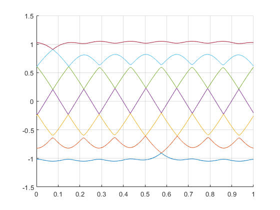
(a) ${\varepsilon}=0.1$

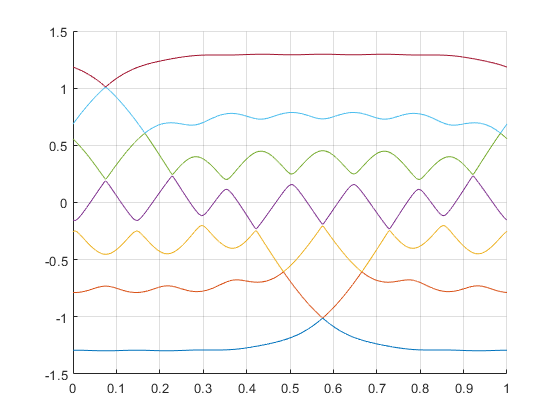
(b) ${\varepsilon}=0.3$

Figure 8. Eigenvalue parameterizations for the cosine potential

Proof.

The remainder of this section is devoted to the proof of Lemma 4.4. We begin with the easier case of a simple resonance, i.e., $s_{0}\geq 4(\log{\varepsilon})^{2}$. Fix any $E_{*}\in{\mathbb{R}}$ with $[E_{*}-\delta_{0},E_{*}+\delta_{0}]\cap[\min V,\max V]\neq\O$, and some $\theta_{*}\in\mathbb{T}$. Then $\mathcal{S}_{0}=\{c^{i}_{0}\}_{i=-\infty}^{\infty}$, and every $c^{i}_{0}$ is contained in a unique level $1$ interval $I^{i}_{1}$, with $|I^{i}_{1}|=\ell_{1}=\lceil\log(1/{\varepsilon})\rceil^{2}$. These are pairwise disjoint by construction, and they may be regular or singular. We discard the regular ones and only consider those $c^{i}_{1}=c^{i}_{0}$ for which $I^{i}_{1}$ is singular. By the definitions,

$$\begin{split}|V(\theta_{*}+k\omega)-E_{*}|&>\delta_{0}\;\forall\;k\in I^{i}_{1}\setminus\{c^{i}_{0}\}\\ |V(\theta_{*}+c^{i}_{0}\omega)-E_{*}|&\leq\delta_{0}\end{split}$$ (4.8)

Let $\{E^{i,1}_{j}(\theta)\}_{j=1}^{\ell_{1}}$ be the eigenvalue parameterizations (Rellich functions) of $H_{I^{i}_{1}}(\theta)$. By min-max, there exists $k(j,\theta)\in I^{i}_{1}$ so that

$$\begin{split}|V(\theta+k(j,\theta)\omega)-E^{i,1}_{j}(\theta)|&\leq 2{\varepsilon}^{2}\quad\forall\;1\leq j\leq\ell_{1}\end{split}$$ (4.9)

Figure 8 exhibits numerically computed Rellich functions for $\ell_{1}=7$ and the cosine potential. The graphs do not cross, but some of the gaps are too small to be visible. Subfigures (A) and (B) show how the gaps become wider with increasing ${\varepsilon}$. The figure demonstrates how we need to jump between different translates $V(\theta+k\omega)$ to approximate any given Rellich graph, hence $k(j,\theta)$, which are not unique near crossing points of $V$ with its own translates by $\omega$. Since $\delta_{1}\ll{\varepsilon}^{2}\ll{\varepsilon}$, (4.3) and (4.8), (4.9) imply that for all $|\theta-\theta_{*}|\ll\delta_{0}$

$$\begin{split}|V(\theta+c^{i}_{0}\omega)-E_{*}|&\ll\delta_{0}\\ |V(\theta+k\omega)-E_{*}|&\gtrsim\delta_{0}\quad\forall\;k\in I^{i}_{1}\setminus\{c^{i}_{0}\}\end{split}$$ (4.10)

with implied absolute constants (depending only on $v,\omega$). We now claim that a normalized eigenfunction $\psi(\theta)$ associated with $H_{I^{i}_{1}}(\theta)\psi(\theta)=E^{i,1}_{j}(\theta)\psi(\theta)$ and $k(j,\theta)=c^{i}_{1}=c^{i}_{0}$ satisfies

$$\begin{split}\|P^{\perp}\psi(\theta)\|_{\ell^{2}(I^{i}_{1})}\lesssim{\varepsilon}^{2}\delta_{0}^{-1}\ll{\varepsilon}\end{split}$$ (4.11)

where $P^{\perp}$ denotes the orthogonal projection onto all vectors perpendicular to $\delta_{c^{i}_{0}}$ in $\ell^{2}(I^{i}_{1})$. Then

$$\begin{split}0&=\psi_{c^{i}_{0}}(\theta)P^{\perp}(H_{I^{i}_{1}}(\theta)-E^{i,1}_{j}(\theta))\delta_{c^{i}_{0}}+P^{\perp}(H_{I^{i}_{1}}(\theta)-E^{i,1}_{j}(\theta))P^{\perp}\psi(\theta)\\ &={\varepsilon}^{2}\psi_{c^{i}_{0}}(\theta)(\delta_{c^{i}_{0}-1}+\delta_{c^{i}_{0}+1})+P^{\perp}(H_{I^{i}_{1}}(\theta)-E^{i,1}_{j}(\theta))P^{\perp}\psi(\theta)\end{split}$$

Here and below we use $\delta$ both for the resonance width and in the Dirac sense, without any danger of confusion. By (4.9) and (4.10),

$$\begin{split}\big{\|}[P^{\perp}(H_{I^{i}_{1}}(\theta)-E^{i,1}_{j}(\theta))P^{\perp}]^{-1}\big{\|}_{\ell^{2}(I^{i}_{1}\setminus\{c^{i}_{0}\})}\lesssim\delta_{0}^{-1}\end{split}$$ (4.12)

which implies (4.11) and

$$\begin{split}|E^{i,1}_{j}(\theta)-V(\theta+c^{i}_{0}\omega)|&=|\langle H_{I^{i}_{1}}(\theta)\psi(\theta),\psi(\theta)\rangle-V(\theta+c^{i}_{0}\omega)|\lesssim{\varepsilon}^{2}\delta_{0}^{-1}\end{split}$$ (4.13)

By first order eigenvalue perturbation (Feynman formula), writing $E=E^{i,1}_{j}$ and $V(\theta)$ for the multiplication operator by the potential,

$$\begin{split}|E^{\prime}(\theta)-V^{\prime}(\theta+c^{i}_{0}\omega)|&=|\langle V^{\prime}(\theta)\psi(\theta),\psi(\theta)\rangle-V^{\prime}(\theta+c^{i}_{0}\omega)|\lesssim{\varepsilon}^{2}\delta_{0}^{-1}\end{split}$$ (4.14)

and by the second order perturbation formula, with $G^{\perp}$ being the resolvent on the left-hand side of (4.12),

$$|E^{\prime\prime}(\theta)-V^{\prime\prime}(\theta+c^{i}_{0}\omega)| =|\langle V^{\prime\prime}(\theta)\psi(\theta),\psi(\theta)\rangle-V^{\prime\prime}(\theta+c^{i}_{0}\omega)-2\langle\psi(\theta),V^{\prime}(\theta)G^{\perp}(E(\theta))V^{\prime}(\theta)\psi(\theta)\rangle|$$

$$\lesssim{\varepsilon}^{2}\delta_{0}^{-1}+({\varepsilon}^{2}\delta_{0})^{2}\delta_{0}^{-1}\lesssim{\varepsilon}^{2}\delta_{0}^{-1}\ll{\varepsilon}$$ (4.15)

The estimates (4.13)-(4.15) hold for $|\theta-\theta_{*}|\ll\delta_{0}$. We conclude from (4.14), (4.15) that

$$\begin{split}\min_{|\theta-\theta_{*}|\ll\delta_{0}}\big{(}|E^{\prime}(\theta)|+|E^{\prime\prime}(\theta)|\big{)}\gtrsim 1\qquad\forall\;\theta_{*}\in\mathbb{T},\end{split}$$ (4.16)

Recall that $E(\theta)=E^{i,1}_{j}(\theta)$ depends on $\theta_{*}$ and $E_{*}$, where the latter is chosen so that $\mathcal{S}_{0}\neq\O$. The constant in (4.16) is uniform in $\theta_{*},E_{*}$. The reader is invited to compare (4.16) to Figure 8.

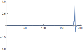
Figure 9. Numerically computed eigenfunctions, ${\varepsilon}=0.3$, $\omega=\sqrt{2}$, $\theta=-17\omega/2$

Now suppose we have two distinct singular intervals $I^{i}_{1}$ and $I^{j}_{1}$ relative to $(\theta_{*},E_{*})$. Then the previous analysis applies to both Rellich functions $E(\theta),\widetilde{E}(\theta)$ defined for $|\theta-\theta_{*}|\ll\delta_{0}$ characterized by

$$\begin{split}\mathrm{spec}(H_{I^{i}_{1}}(\theta))\cap[E_{*}-\delta_{0}/2,E_{*}-\delta_{0}/2]&=\{E(\theta)\},\\ \mathrm{spec}(H_{I^{j}_{1}}(\theta))\cap[E_{*}-\delta_{0}/2,E_{*}-\delta_{0}/2]&=\{\widetilde{E}(\theta)\}\end{split}$$ (4.17)

By (4.3) we have $|E(\theta_{*})-E_{*}|\leq\delta_{1}$, $|\widetilde{E}(\theta_{*})-E_{*}|\leq\delta_{1}$. By (4.9) we have

$$|V(\theta_{*}+c^{i}_{0}\omega)-E(\theta_{*})|\leq 2{\varepsilon}^{2},\quad|V(\theta_{*}+c^{j}_{0}\omega)-\widetilde{E}(\theta_{*})|\leq 2{\varepsilon}^{2}$$

whence

$$|V(\theta_{*}+c^{i}_{0}\omega)-V(\theta_{*}+c^{j}_{0}\omega)|\leq 4{\varepsilon}^{2}+2\delta_{1}\leq 5{\varepsilon}^{2}$$

We showed in Lemma 4.2 that this implies

$$\begin{split}m(c^{i}_{0},c^{j}_{0})\lesssim{\varepsilon}\ll\delta_{0}.\end{split}$$ (4.18)

Next, we improve this estimate to to $m(c^{i}_{0},c^{j}_{0})\lesssim\delta_{1}$. Suppose (4.18) means $\|(c^{i}_{0}-c^{j}_{0})\omega\|\ll\delta_{0}$. By (3.2) one has

$$\begin{split}H_{I^{i}_{1}}(\theta)=H_{I^{j}_{1}}(\theta+(c^{i}_{0}-c^{j}_{0})\omega)\end{split}$$ (4.19)

which, combined with (4.17) implies that $\widetilde{E}(\theta)=E(\theta+(c^{j}_{0}-c^{i}_{0})\omega)$ for all $|\theta-\theta_{*}|\ll\delta_{0}$. This finally implies that

$$|E(\theta_{*})-E(\theta_{*}+(c^{j}_{0}-c^{i}_{0})\omega)|\leq 2\delta_{1}$$

From (4.16) we obtain $\|(c^{j}_{0}-c^{i}_{0})\omega\|^{2}\lesssim\delta_{1}$. On the other hand, if (4.18) means $\|2\theta_{*}+(c^{i}_{0}+c^{j}_{0})\omega\|\ll\delta_{0}$, then we have

$$\begin{split}\widetilde{E}(\theta)=E(2\theta_{*}-\theta-\theta_{**}),\quad\theta_{**}:=2\theta_{*}+(c^{i}_{0}+c^{j}_{0})\omega\end{split}$$ (4.20)

for all $|\theta-\theta_{*}|\ll\delta_{0}$. In terms of Figure 3 this corresponds to $E(\theta)$ being approximated by $V$ over $J_{1}$, whereas $\widetilde{E}(\theta)$ is approximated by $V$ over $J_{2}$. Setting $\theta=\theta_{*}$ in (4.20), we find that

$$|E(\theta_{*})-E(\theta_{*}-\theta_{**})|\leq 2\delta_{1}$$

which implies $\|\theta_{**}\|^{2}\lesssim\delta_{1}$. We have thus proved Lemma 4.4 for simple resonances.

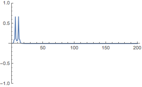
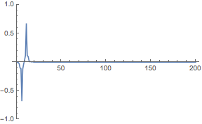
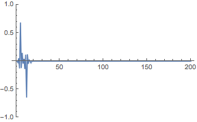
Figure 10. Numerically computed eigenfunctions, ${\varepsilon}=0.3$, $\omega=\sqrt{2}$, $\theta=-17\omega/2$

Figures 9 and 10 depict eigenfunctions on finite volume $200$ computed with Mathematica (the code is included in the appendix for the reader to experiment for themselves, for example by changing $\theta$ or trying rational $\omega$). The choice of $\theta$ was made as a crossing point of $V$ with one of its translates by a multiple of $\omega$, since double resonances occur near those points. The first eigenfunction shown in the upper left of Figures 9 shows the case of a simple resonance, whereas the second and third are more complicated – they exhibit a main peak with smaller ones due to resonances at later stages of the induction. On the other hand, Figure 10 exhibits double resonances quite clearly (with the bottom eigenfunction exhibiting a more complicated structure). The reader should note the distinct distribution of the $\ell^{2}$-mass which is quite apparent on the $y$-axes of these figures.

We now prove Lemma 4.4 for double resonances. Let $I^{i}_{1}$ be singular (as the red interval on the right-hand side of Figure 5), centered at $c^{i}_{1}=\frac{1}{2}(c^{2i}_{0}+c^{2i+1}_{0})\in\frac{1}{2}\mathbb{Z}$. As a side remark, suppose that $c^{i}_{1}\in\frac{1}{2}+\mathbb{Z}$. Then all $c^{j}_{1}\in\frac{1}{2}+\mathbb{Z}$ due to $c^{2j+1}_{0}-c^{2j}_{0}=\mathrm{const}.$ for all $j$ (since we passed to $\bar{\mathcal{S}}_{0}$). At the next levels $n=2,3,\ldots,N$ we will encounter only simple resonances, and so all $c^{k}_{n}\in\frac{1}{2}+\mathbb{Z}$ for all these $n$. If we then encounter a double resonance at $N+1$, it implies that $c^{k}_{N+1}\in\frac{1}{2}\mathbb{Z}$, and the patter repeats itself. Continuing with the main argument, one then has

$$\begin{split}&|V(\theta_{*}+c^{2i}_{0}\omega)-E_{*}|\lesssim\delta_{0},\quad|V(\theta_{*}+c^{2i+1}_{0}\omega)-E_{*}|\lesssim\delta_{0}\\ &|V(\theta_{*}+k\omega)-E_{*}|\gg\delta_{0}^{\frac{1}{2}}\quad\forall\;k\in I^{i}_{1}\setminus\{c^{2i}_{0},c^{2i+1}_{0}\}\end{split}$$

where the second line follows from the Diophantine condition since $I^{i}_{1}=\lceil\log(1/{\varepsilon})\rceil^{4}$ (one can choose a larger lower bound such as $\delta_{0}^{a}$ for any fixed $0<a\leq\frac{1}{2}$ at the expense of making ${\varepsilon}$ smaller). By (4.9),

$$\begin{split}\mathrm{spec}(H_{I^{i}_{1}}(\theta))\cap[E_{*}-\delta_{0}^{\frac{1}{2}},E_{*}+\delta_{0}^{\frac{1}{2}}]=\{E(\theta),\widetilde{E}(\theta)\}\quad\forall\;|\theta-\theta_{*}|\lesssim\delta_{0}^{\frac{1}{2}}\end{split}$$ (4.21)

with $E>\widetilde{E}$. By the same type of argument as in the simple resonant case, cf. (4.11), (4.12), we see that the normalized eigenfunctions of $H_{I^{i}_{1}}(\theta)$ associated with $E$, resp. $\widetilde{E}$, are

$$\begin{split}\psi&=A\delta_{c^{2i}_{0}}+B\delta_{c^{2i+1}_{0}}+O({\varepsilon}^{2}\delta_{0}^{-\frac{1}{2}})\\ \widetilde{\psi}&=-B\delta_{c^{2i}_{0}}+A\delta_{c^{2i+1}_{0}}+O({\varepsilon}^{2}\delta_{0}^{-\frac{1}{2}})\end{split}$$ (4.22)

uniformly on $|\theta-\theta_{*}|\leq\delta_{0}^{\frac{1}{2}}$ with $A^{2}+B^{2}=1$. In place of (4.12) we have

$$\begin{split}\big{\|}[P^{\perp}(H_{I^{i}_{1}}(\theta)-E_{*})P^{\perp}]^{-1}\big{\|}_{\ell^{2}(I^{i}_{1}\setminus\{c^{2i}_{0},c^{2i+1}_{0}\})}\lesssim\delta_{0}^{-\frac{1}{2}}\end{split}$$ (4.23)

where $P^{\perp}$ is the orthogonal projection perpendicular to $\mathrm{span}(\delta_{c^{2i}_{0}},\delta_{c^{2i+1}_{0}})$ in $\ell^{2}(I^{i}_{1})$. The eigenvalues at level $0$ associated with the points $c^{2i}_{0}$, $c^{2i+1}_{0}$ are, resp., $E^{2i}_{0}(\theta):=V(\theta+c^{2i}_{0}\omega)$, $E^{2i+1}_{0}(\theta):=V(\theta+c^{2i+1}_{0}\omega)$. This terminology is justified by the relations

$$\langle H(\theta)\delta_{c^{2i}_{0}},\delta_{c^{2i}_{0}}\rangle=E^{2i}_{0}(\theta),\quad\langle H(\theta)\delta_{c^{2i+1}_{0}},\delta_{c^{2i+1}_{0}}\rangle=E^{2i+1}_{0}(\theta)$$

By Lemma 4.2, $\|\theta_{**}\|\lesssim\delta_{0}^{\frac{1}{2}}$ with $\theta_{**}=2\theta_{*}+(c^{2i}_{0}+c^{2i+1}_{0})\omega=2(\theta_{*}+c^{i}_{1}\omega)$. It follows that either (a) $\|\theta_{*}+c^{i}_{1}\omega\|\lesssim\delta_{0}^{\frac{1}{2}}$ or (b) $\|\theta_{*}+\frac{1}{2}+c^{i}_{1}\omega\|\lesssim\delta_{0}^{\frac{1}{2}}$. These relations show that the unique solution of $E^{2i}_{0}(\theta)=E^{2i+1}_{0}(\theta)$ on $|\theta-\theta_{*}|\lesssim\delta_{0}^{\frac{1}{2}}$ is either (a) $\theta_{s}=-c^{i}_{1}\omega$ or (b) $\theta_{s}=\frac{1}{2}-c^{i}_{1}\omega$ (henceforth, $\theta_{s}$ will mean either of these whichever applies). These identities are a restatement of $V$ being symmetric both (a) around $0$ and (b) around $\frac{1}{2}$. Furthermore, one has

$$E_{0}^{2i}(\theta+\theta_{s})=E_{0}^{2i+1}(-\theta+\theta_{s})$$

whence $\partial_{\theta}E_{0}^{2i}(\theta_{s})=-\partial_{\theta}E_{0}^{2i+1}(\theta_{s})$.

Figure 11. Crossing graphs and double resonance

The configuration associated with a double resonance is shown in Figure 11. Not only do the segments of the $V$-graphs (i.e., $E^{2i}_{0}$ and $E^{2i+1}_{0}$) intersect at $\theta_{s}$, but $E,\widetilde{E}$ have their critical point at $\theta_{s}$ within the interval $|\theta-\theta_{*}|\lesssim\delta_{0}^{\frac{1}{2}}$. Indeed,

$$H_{I^{i}_{1}}(\theta+\theta_{s})=UH_{I^{i}_{1}}(-\theta+\theta_{s})U$$

where $U$ is the reflection on $\mathbb{Z}$ about $c^{i}_{1}\in\frac{1}{2}\mathbb{Z}$. In particular, the eigenvalues are the same. In fact, using (4.21) one concludes that

$$\begin{split}E(\theta+\theta_{s})=E(-\theta+\theta_{s}),\quad\widetilde{E}(\theta+\theta_{s})=\widetilde{E}(-\theta+\theta_{s})\quad\forall\;|\theta-\theta_{*}|\lesssim\delta_{0}^{\frac{1}{2}}\end{split}$$ (4.24)

whence $E^{\prime}(\theta_{s})=\widetilde{E}(\theta_{s})=0$.

Next, we establish the lower bound

$$\begin{split}E(\theta)-\widetilde{E}(\theta)>(c{\varepsilon})^{5\ell_{1}^{1/2}}\gg\delta_{1}={\varepsilon}^{\ell_{1}^{2/3}}={\varepsilon}^{|\log{\varepsilon}|^{8/3}}\end{split}$$ (4.25)

which follows immediately from this separation lemma, see [FroSpeWit, Lemma 4.1]. This spectral gap is much larger than the resonance width $\delta_{1}$.

Lemma 4.6.

Let $H_{\Lambda}\psi_{j}=E_{j}\psi_{j}$, $j=1,2$ with nontrivial $\psi_{j}$. If $\|\psi_{j}\|_{\ell^{2}(\Lambda_{0})}\geq\frac{1}{2}\|\psi_{j}\|_{\ell^{2}(\Lambda)}$ for $j=1,2$ with $\Lambda_{0}\subset\Lambda$ and $|\Lambda_{0}|\geq 2$, then

$$\begin{split}|E_{1}-E_{2}|\geq(c_{1}{\varepsilon})^{|\Lambda_{0}|}({\varepsilon}^{-2}+|\Lambda_{0}|)^{-1}\end{split}$$ (4.26)

with a constant $c_{1}=c_{1}(v)>0$.

Proof.

Let $\Lambda_{0}=[n_{0}-\ell_{0},n_{0}+\ell_{0}]$ or $\Lambda_{0}=[n_{0}-\ell_{0},n_{0}+\ell_{0}-1]$. By assumption, $\ell_{0}\geq 1$. Normalize $\psi_{j}(n_{0}-1)^{2}+\psi_{j}(n_{0})^{2}=1$ for $j=1,2$. Setting $\widetilde{\psi}_{1}(n)=\psi_{1}(n)$ if $n\in\Lambda$, $n\geq n_{0}$ and $\widetilde{\psi}_{1}(n)=-\psi_{1}(n)$ if $n\in\Lambda$, $n<n_{0}$ one obtains from considering $\langle H_{\Lambda}\widetilde{\psi}_{1},\psi_{2}\rangle=\langle\widetilde{\psi}_{1},H_{\Lambda}\psi_{2}\rangle$ that

$$\begin{split}2{\varepsilon}^{2}|\vec{v}_{1}\wedge\vec{v}_{2}|&=2{\varepsilon}^{2}|\psi_{1}(n_{0})\psi_{2}(n_{0}-1)-\psi_{2}(n_{0})\psi_{1}(n_{0}-1)|=\\ &\leq 2|E_{1}-E_{2}|(\|\psi_{1}\|_{2}\|\psi_{2}\|_{2})^{\frac{1}{2}}(\|\psi_{1}\|_{\ell^{2}(\Lambda_{0})}\|\psi_{2}\|_{\ell^{2}(\Lambda_{0})})^{\frac{1}{2}}\\ &\leq 2(C{\varepsilon}^{-2})^{\ell_{0}}\,|E_{1}-E_{2}|(\|\psi_{1}\|_{2}\|\psi_{2}\|_{2})^{\frac{1}{2}}\end{split}$$ (4.27)

where $\vec{v}_{j}=\binom{\psi_{j}(n_{0})}{\psi_{j}(n_{0}-1)}$ and $C=C(v)$. The final estimate is obtained from the transfer matrix representation of the eigenfunctions, viz. for $n\geq n_{0}+1$

$$\binom{\psi_{j}(n)}{\psi_{j}(n-1)}=\prod_{k=n_{0}}^{n-1}\left[\begin{matrix}{\varepsilon}^{-2}(v_{k}-E_{j})&-1\\ 1&0\end{matrix}\right]\vec{v}_{j}$$

and for $n\leq n_{0}-1$

$$\binom{\psi_{j}(n-1)}{\psi_{j}(n)}=\prod_{k=n_{0}-1}^{n}\left[\begin{matrix}{\varepsilon}^{-2}(v_{k}-E_{j})&-1\\ 1&0\end{matrix}\right]^{-1}\vec{v}_{j}$$

On the one hand, with $B=C{\varepsilon}^{-2}$, and using that $\|\vec{v}_{1}-\vec{v}_{2}\|_{2}=2|\vec{v}_{1}\wedge\vec{v}_{2}|$,

$$\begin{split}\|\psi_{1}-\psi_{2}\|_{\ell^{2}(\Lambda_{0})}&\leq 2B^{\ell_{0}}|\vec{v}_{1}\wedge\vec{v}_{2}|+\ell_{0}B^{\ell_{0}}|E_{1}-E_{2}|\\ &\leq 2{\varepsilon}^{-2}B^{\ell_{0}}\,|E_{1}-E_{2}|(\|\psi_{1}\|_{2}\|\psi_{2}\|_{2})^{\frac{1}{2}}+\ell_{0}B^{\ell_{0}}|E_{1}-E_{2}|\end{split}$$

On the other hand, with $a_{j}:=\|\psi_{j}\|_{\ell^{2}(\Lambda)}$,

$$\begin{split}\sqrt{a_{1}^{2}+a_{2}^{2}}&\leq\frac{1}{2}(a_{1}+a_{2})+\|\psi_{1}-\psi_{2}\|_{\ell^{2}(\Lambda_{0})}\\ &\leq\frac{1}{2}(a_{1}+a_{2})+B^{\ell_{0}}(B\sqrt{a_{1}a_{2}}+\ell_{0})|E_{1}-E_{2}|\\ &\leq\frac{1}{2}(a_{1}+a_{2})+B^{\ell_{0}}(B+\ell_{0})|E_{1}-E_{2}|\,\sqrt{a_{1}a_{2}}\end{split}$$

If $|E_{1}-E_{2}|<\frac{1}{4}B^{-\ell_{0}}(B+\ell_{0})^{-1}$, then $\sqrt{a_{1}^{2}+a_{2}^{2}}<\frac{5}{8}(a_{1}+a_{2})$ which is impossible. Adjusting the constants one obtains (4.26). ∎

The critical points of $V$ are $\theta=0$ and $\theta=\frac{1}{2}$. We claim that $\min(\|\theta_{*}\|,\|\theta_{*}-\frac{1}{2}\|)\geq K\delta_{0}^{\frac{1}{2}}$ where $K$ is any large constant, to be fixed below (as always, provided ${\varepsilon}$ is small enough). This is immediate from the Diophantine condition due to $s_{0}\leq 4(\log{\varepsilon})^{2}$, cf. Figure 3. In particular, $|V^{\prime}(\theta)|\gg\delta_{0}^{\frac{1}{2}}$ on the interval $|\theta-\theta_{*}|\lesssim\delta_{0}^{\frac{1}{2}}$. By first order eigenvalue perturbation and (4.22), uniformly on this interval

$$\partial_{\theta}E(\theta)=\langle\psi(\theta),V^{\prime}(\theta)\psi(\theta)\rangle=A^{2}(\theta)\partial_{\theta}E^{2i}_{0}(\theta)+B^{2}(\theta)\partial_{\theta}E^{2i+1}_{0}(\theta)+O({\varepsilon}^{2}\delta_{0}^{-\frac{1}{2}})$$

where by the preceding $|\partial_{\theta}E^{2i}_{0}(\theta)|\gg\delta_{0}^{\frac{1}{2}}$ and $|\partial_{\theta}E^{2i+1}_{0}(\theta)|\gg\delta_{0}^{\frac{1}{2}}$. Setting $\theta=\theta_{s}$ it follows that $A^{2}(\theta_{s})-B^{2}(\theta_{s})=O({\varepsilon}^{2}\delta_{0}^{-1})=O({\varepsilon})$. Due to $A^{2}+B^{2}=1$, $|A(\theta_{s})|^{2}=1/2-O({\varepsilon})$ and $|B(\theta_{s})|^{2}=1/2-O({\varepsilon})$. In fact, the same argument shows that $|A(\theta)|\simeq|B(\theta)|\simeq 1$ for all $|\theta-\theta_{*}|\lesssim\delta_{0}^{\frac{1}{2}}$ with $|\partial_{\theta}E(\theta)|\lesssim\delta_{0}^{\frac{1}{2}}$.

Using this property we can now establish closeness of all eigenvalues. In fact, $H_{\Lambda}(\theta)\psi(\theta)=E(\theta)\psi(\theta)$ and $H_{\Lambda}(\theta)\widetilde{\psi}(\theta)=\widetilde{E}(\theta)\widetilde{\psi}(\theta)$ in combination with (4.22) imply that

$$\begin{split}E^{2i}_{0}(\theta)-E(\theta)=O({\varepsilon}^{2}\delta_{0}^{-\frac{1}{2}}),\quad E^{2i+1}_{0}(\theta)-E(\theta)=O({\varepsilon}^{2}\delta_{0}^{-\frac{1}{2}})\end{split}$$ (4.28)

and the same for $\widetilde{E}$. In particular,

$$\begin{split}|E(\theta)-\widetilde{E}(\theta)|\lesssim{\varepsilon}^{2}\delta_{0}^{-\frac{1}{2}}\end{split}$$ (4.29)

for all $|\theta-\theta_{*}|\lesssim\delta_{0}^{\frac{1}{2}}$ with $|\partial_{\theta}E(\theta)|\lesssim\delta_{0}^{\frac{1}{2}}$. The final step in our analysis is to establish a lower bound on $|\partial_{\theta}^{2}E(\theta)|$ and $|\partial_{\theta}^{2}\widetilde{E}(\theta)|$ for those $\theta$. This hinges on the second order perturbation formulas (suppressing $\theta$ as argument)

$$\begin{split}\partial_{\theta}^{2}E&=\langle\psi,V^{\prime\prime}\psi\rangle-2\langle V^{\prime}\psi,G(E)^{\perp}V^{\prime}\psi\rangle\\ \partial_{\theta}^{2}\widetilde{E}&=\langle\widetilde{\psi},V^{\prime\prime}\widetilde{\psi}\rangle-2\langle V^{\prime}\widetilde{\psi},G(\widetilde{E})^{\perp}V^{\prime}\widetilde{\psi}\rangle\end{split}$$

on $\ell^{2}(I^{i}_{1})$ with $G(E)^{\perp}=[P^{\perp}_{\psi}(H_{I^{i}_{1}}-E)P^{\perp}_{\psi}]^{-1}$ in $P^{\perp}_{\psi}\ell^{2}(I^{i}_{1})$ and $P^{\perp}_{\psi}$ being the orthogonal projection onto the complement of $\psi$ in $\ell^{2}(I^{i}_{1})$. Analogous comments apply $G(\widetilde{E})^{\perp}$ which is the resolvent orthogonal to $\widetilde{\psi}$. We now write

$$\langle V^{\prime}\psi,G(E)^{\perp}V^{\prime}\psi\rangle=\frac{\langle\psi,V^{\prime}\widetilde{\psi}\rangle^{2}}{\widetilde{E}-E}+\langle V^{\prime}\psi,G(E)^{\perp\perp}V^{\prime}\psi\rangle$$

where $G(E)^{\perp\perp}=P^{\perp}_{\widetilde{\psi}}[P^{\perp}_{\psi}(H_{I^{i}_{1}}-E)P^{\perp}_{\psi}]^{-1}P^{\perp}_{\widetilde{\psi}}$. By (4.21), $\|G(E)^{\perp\perp}\|\lesssim\delta_{0}^{-\frac{1}{2}}$. On the other hand, by (4.22)

$$\langle\psi,V^{\prime}\widetilde{\psi}\rangle=-2AB\partial_{\theta}E^{2i}_{0}(\theta_{s})+O(\delta_{0}^{\frac{1}{2}})$$

whence from $|AB|\simeq 1$,

$$|\langle\psi,V^{\prime}\widetilde{\psi}\rangle|\gg\delta_{0}^{\frac{1}{2}}$$

Combining this with (4.29) we obtain

$$|\langle V^{\prime}\psi,G(E)^{\perp}V^{\prime}\psi\rangle|\gg{\varepsilon}^{-2}\delta_{0}^{\frac{3}{2}}-O(\delta_{0}^{-\frac{1}{2}})\gg{\varepsilon}^{-2}\delta_{0}^{\frac{3}{2}}\gg 1$$

Since $|\langle\psi,V^{\prime\prime}\psi\rangle|\lesssim 1$, it follows that

$$\begin{split}|\partial_{\theta}^{2}E(\theta)|\gg{\varepsilon}^{-2}\delta_{0}^{\frac{3}{2}},\quad|\partial_{\theta}^{2}\widetilde{E}(\theta)|\gg{\varepsilon}^{-2}\delta_{0}^{\frac{3}{2}}\end{split}$$ (4.30)

for all $|\theta-\theta_{*}|\lesssim\delta_{0}^{\frac{1}{2}}$ with $|\partial_{\theta}E(\theta)|\lesssim\delta_{0}^{\frac{1}{2}}$. The exact same analysis applies to $\widetilde{E}$. To summarize, these are the main points concerning double resonances at level $1$.

• $s_{0}\leq(\log{\varepsilon})^{2}$ and the level-$0$ singular sites are $\mathcal{S}_{0}=\{c^{j}_{0}\}_{j=-\infty}^{\infty}$ with $c^{2i+1}_{0}-c^{2i}_{0}=s_{0}$ for all $i$. We have $|V(\theta+k\omega)-E_{*}|\lesssim\delta_{0}^{\frac{1}{2}}$ for $k\in\{c^{2i}_{0},c^{2i+1}_{0}\}$, $|V(\theta+k\omega)-E_{*}|\gg\delta_{0}^{\frac{1}{2}}$ for all $k\in I^{i}_{1}\setminus\{c^{2i}_{0},c^{2i+1}_{0}\}$, both for all $|\theta-\theta_{*}|\lesssim\delta_{0}^{\frac{1}{2}}$. Here $I^{i}_{1}\subset\mathbb{Z}$, $|I^{i}_{1}|\simeq(\log{\varepsilon})^{4}$, centered at $c^{i}_{1}\in\frac{1}{2}\mathbb{Z}$ and $\mathrm{dist}(\mathrm{spec}(H_{I^{i}_{1}}(\theta_{*})),E_{*})\lesssim\delta_{1}={\varepsilon}^{\ell_{1}^{2/3}}$.

• $\mathrm{spec}(H_{I^{i}_{1}}(\theta))\cap[E_{*}-\delta_{0}^{\frac{1}{2}},E_{*}+\delta_{0}^{\frac{1}{2}}]=\{E(\theta),\widetilde{E}(\theta)\}$ (with $E>\widetilde{E}$) for these $\theta$, with all other eigenvalues being separated from $E_{*}$ by $\gg\delta_{0}^{\frac{1}{2}}$. From the level-$0$ estimate $m(c^{2i}_{0},c^{2i+1}_{0})\lesssim\delta_{0}$, either $\theta_{s}=-c^{i}_{1}\omega$ or $\theta_{s}=\frac{1}{2}-c^{i}_{1}\omega$ satisfy $\|\theta_{s}-\theta_{*}\|\lesssim\delta_{0}^{\frac{1}{2}}$ and the unique critical points of $E,\widetilde{E}$ in this interval are at $\theta_{s}$. There is a spectral gap of size $E(\theta)-\widetilde{E}(\theta)>{\varepsilon}^{5\ell_{1}^{\frac{1}{2}}}$.

• For every $|\theta-\theta_{*}|\lesssim\delta_{0}^{\frac{1}{2}}$ one has either both $|\partial_{\theta}E(\theta)|\gg\delta_{0}^{\frac{1}{2}}$ and $|\partial_{\theta}\widetilde{E}(\theta)|\gg\delta_{0}^{\frac{1}{2}}$ (large slopes), or both $|\partial_{\theta}E(\theta)|\lesssim\delta_{0}^{\frac{1}{2}}$ and $|\partial_{\theta}\widetilde{E}(\theta)|\lesssim\delta_{0}^{\frac{1}{2}}$ (small slopes). This follows from $|\partial_{\theta}E_{0}^{2i}(\theta_{s})|\gg\delta_{0}^{\frac{1}{2}}$, and the first order eigenvalue perturbation formulas

  $$\begin{split}\partial E(\theta)&=(A^{2}(\theta)-B^{2}(\theta))\partial_{\theta}E_{0}^{2i}(\theta_{s})+O(\delta_{0}^{\frac{1}{2}})\\ \partial\widetilde{E}(\theta)&=(-A^{2}(\theta)+B^{2}(\theta))\partial_{\theta}E_{0}^{2i}(\theta_{s})+O(\delta_{0}^{\frac{1}{2}})\end{split}$$

  for all $|\theta-\theta_{*}|\lesssim\delta_{0}^{\frac{1}{2}}$, cf. (4.22).

• If the small slope alternative occurs, then $|A(\theta)|\simeq|B(\theta)|\simeq 1$ and (4.28) holds for both $E$ and $\widetilde{E}$. In particular, the spectral gap is small as in (4.29), and the second derivatives are large and $\gg\delta_{0}^{-\frac{1}{2}}$, see (4.30). This means that the intervals of small slopes around the critical points at $\theta_{s}$ are of size $\ll\delta_{0}$.

• Figure 11 depicts the situation for a double resonance: $E$ reaches its minimum, resp. $\widetilde{E}$ its maximum, at $\theta_{s}$. The spectral gap is the smallest at this point and the quantitative estimates above hold. In particular, this gap is much larger than $\delta_{1}$, whence exactly one of $E$ or $\widetilde{E}$ achieve the resonance condition (4.3) at $\theta_{*}$.

To conclude the proof of Lemma 4.4 we apply this description to two such level $1$ intervals, say $I^{i}_{1}$ and $I^{j}_{1}$. Because of the double resonance assumption, we have

$$\|1/2+c^{i}_{1}\omega\|+\|1/2+c^{j}_{1}\omega\|\lesssim\delta_{0}^{\frac{1}{2}}$$

which implies that $m(c^{i}_{1},c^{j}_{1})=\|(c^{i}_{1}-c^{j}_{1})\omega\|\lesssim\delta_{0}^{\frac{1}{2}}$. As in the single resonance case, cf. (4.19), for all $|\theta-\theta_{*}|\lesssim\delta_{0}^{\frac{1}{2}}$

$$H_{I^{i}_{1}}(\theta)=H_{I^{j}_{1}}(\theta+(c^{i}_{1}-c^{j}_{1})\omega)\text{\ and\ }E^{i}_{1}(\theta)=E^{j}_{1}(\theta+(c^{i}_{1}-c^{j}_{1})\omega),\;\widetilde{E}^{i}_{1}(\theta)=\widetilde{E}^{j}_{1}(\theta+(c^{i}_{1}-c^{j}_{1})\omega)$$

Finally, by (4.3), either

$$|E^{j}_{1}(\theta_{*})-E^{j}_{1}(\theta_{*}+(c^{i}_{1}-c^{j}_{1})\omega)|\lesssim\delta_{1}\text{\ or \ }|\widetilde{E}^{j}_{1}(\theta_{*})-\widetilde{E}^{j}_{1}(\theta_{*}+(c^{i}_{1}-c^{j}_{1})\omega)|\lesssim\delta_{1}$$

By the bounds derived above on the first and second derivatives on $E^{i}_{1}$ etc. and elementary calculus, we finally conclude that $m(c^{i}_{1},c^{j}_{1})\lesssim\delta_{1}^{\frac{1}{2}}$. Indeed, in the large slopes case, $m(c^{i}_{1},c^{j}_{1})=\|(c^{i}_{1}-c^{j}_{1})\omega\|\lesssim\delta_{0}^{-\frac{1}{2}}\delta_{1}$, whereas in the small slopes case, $m(c^{i}_{1},c^{j}_{1})\lesssim\delta_{0}^{\frac{1}{4}}\delta_{1}^{\frac{1}{2}}$. This is slightly better than what Lemma 4.4 claims, and we are done. ∎

The full induction needed to establish (4.5) follows these exact same lines with no essentially new ideas needed. The reader can either convince themselves of this fact, or consult [FroSpeWit]. Note, however, that Lemma 5.2 in loc. cit.  erroneously sets $\theta_{s}=-c^{i}_{m}\alpha$ forgetting the case (b) above in which $1/2$ has to be added. This is a systematic oversight in Section 5 in that paper which is rooted in a false identity at the conclusion of the proof of Lemma 5.3: $2\|\theta\|=\|2\theta\|$ for the metric on $\mathbb{T}$.

It seems very difficult to approach quasi-periodic localization in more general settings by relying on eigenvalue parametrization, as we did in this section.

4.2. The work of Forman and VandenBoom: dropping evenness of $V$

We will now discuss the highly challenging task of implementing some version of the Fröhlich-Spencer-Wittwer proof strategy without the symmetry assumption on the potential. This has recently been accomplished by Forman and VandenBoom, see [ForVan]. We now sketch the proof of their result.

Theorem 4.7.

Let $V\in C^{2}(\mathbb{T})$ have exactly two nondegenerate critical points. Define

$$H_{\varepsilon}(\theta)=\varepsilon^{2}\Delta_{\mathbb{Z}}+V_{\theta},\quad V_{\theta}(n)=V(T_{\omega}^{n}\theta)\;\forall\,n\in\mathbb{Z}$$ (4.31)

where $\omega\in\mathbb{T}$ is Diophantine, viz. $\|n\omega\|\geq c_{0}n^{-2}$ for all $n\geq 1$ with some $c_{0}>0$. There exists $\varepsilon_{0}(c_{0},V)$ such that for all $0<\varepsilon\leq\varepsilon_{0}$ the operators $H_{\theta,\varepsilon}$ exhibit Anderson localization for a.e. $\theta\in\mathbb{T}$.

This is precisely the result of Fröhlich, Spencer, and Wittwer without the evenness assumption, and we will make frequent references to the proof of that result. See the previous section.

As in the symmetric case, we can define singular sites $\mathcal{S}_{0}$ relative to $\theta_{*},E_{*}$. However, the $m(k,\ell)$ function is no longer useful, as $\|2\theta_{*}+(k+\ell)\omega\|$ is no longer small if $T^{k}_{\omega}\theta_{*}$ and $T^{\ell}_{\omega}\theta_{*}$ fall into different connected components of $V^{-1}([E_{*}-\delta_{0},E_{*}+\delta_{0}])$. Without symmetry, no such function $m$ can be defined to be independent of $E_{*}$.

Figure 12. A cartoon output of the first inductive step: a collection $\mathcal{E}_{1}$ of Rellich functions of various Dirichlet restrictions of $H$, whose domains (and their relevant translates) cover the circle $\mathbb{T}$. The curves in black come from double resonances, and the curves in gray are simple resonant.

Instead, we divide the energy axis into several overlapping intervals, and we construct a collection $\mathcal{E}_{1}$ of well-separated Rellich functions of certain Dirichlet restrictions of $H$ whose domains cover the circle $\mathbb{T}$ with the same structural properties as $\mathbf{E}_{0}$, cf. Figure 12. We choose an initial interval length $\ell_{1}^{(1)}$ and consider energy regions of size $\mathcal{O}((\ell_{1}^{(1)})^{-16})$. Each energy region can be characterized as double-resonant, if it contains some $E_{n}$ which satisfies $E_{n}=V(\theta_{n})=V(\theta_{n}+n\omega)$ for some $\theta\in\mathbb{T}$ and $|n|\leq\ell_{1}^{(1)}$, or simple-resonant if it does not. Each function $\mathbf{E}_{1}\in\mathcal{E}_{1}$ is a Rellich function of $H_{\Lambda_{1}}$, where $\Lambda_{1}\subset\mathbb{Z}$ is an interval of length $\ell_{1}^{(1)}$ if the energy region is simple-resonant, or $\ell_{1}^{(2)}\approx\left(\ell_{1}^{(1)}\right)^{2}$ if the energy region is double-resonant. The singular intervals are then characterized by

$$\mathcal{S}_{1}=\{\Lambda_{1}+m\,|\,m\in\mathbb{Z},\,|\mathbf{E}_{1}(\theta_{*}+m\omega)-E_{*}|<\delta_{1}\}$$

where $\mathbf{E}_{1}\in\mathcal{E}_{1}$ is the Rellich function defined in the energy region containing $E_{*}$, and $\delta_{1}$ is defined as Fröhlich, Spencer, and Wittwer define it.

Assuming the constructed Rellich functions satisfy a Morse condition, maintain two monotonicity intervals, and are well-separated from other Rellich functions on the same domain (i.e., we have an upper bound on $\|[P^{\perp}(H_{\Lambda_{1}}-\mathbf{E}_{1})P^{\perp}]^{-1}\|$, as considered above), we can iterate this procedure inductively and conclude the proof as Fröhlich, Spencer, and Wittwer do. While we cannot control the bad set of $\theta\in\mathbb{T}$ by the $m$ function as they do, we can bound it by controlling the number of Rellich functions we construct in $\mathcal{E}_{n}$ at each scale. Since the energy regions at scale $s$ are of size at least $\mathcal{O}(\delta_{s-2}^{3})$, each energy region at scale $s-1$ gives rise to at most $\mathcal{O}(\delta_{s-2}^{-3})$ Rellich functions at scale $s$; thus, we inductively bound $|\mathcal{E}_{n}|\leq\mathcal{O}(\delta_{n-2}^{-4})$. The bad set of $\theta$ at scale $n$ for a specific $\mathbf{E}_{n}\in\mathcal{E}_{n}$ is bounded in measure by $\ell_{n+1}^{2}\delta_{n-1}^{1/4}$ by a calculus argument. Since $\delta_{n-2}^{-4}\ell_{n+1}^{2}\delta_{n-1}^{1/4}$ is still summable, we can apply Borel-Cantelli.

It remains to show that the Rellich functions in $\mathcal{E}_{n+1}$ inherit the structural properties of those in $\mathcal{E}_{n}$; namely, a Morse condition and a uniform separation estimate. By construction, simple resonant Rellich functions are well-separated from others, so they satisfy $\|\mathbf{E}_{n+1}-\mathbf{E}_{n}\|_{C^{2}}\ll\delta_{n}$ by the same arguments used above. In the double-resonant case, the Morse lower bound on the second derivative follows by a slight modification of the above argument to allow for $V$’s asymmetry. A new argument is required to separate the pair of double-resonant Rellich functions uniformly by a stable, quantifiable gap. We thus show

Lemma 4.8.

In our setting, double resonances of a Rellich function $\mathbf{E}_{n}$ of $H_{\Lambda_{n}}$ resolve as a pair of uniformly locally separated Morse Rellich functions $\mathbf{E}_{n+1,\vee}>\mathbf{E}_{n+1,\wedge}$ of $H_{\Lambda_{n+1}}$ with at most one critical point, cf. Figure 13. The size of the gap is larger than the next resonance scale:

$$\inf\mathbf{E}_{n+1,\vee}-\sup\mathbf{E}_{n+1,\wedge}\gg\delta_{n+1}$$

This gap ensures that any Rellich function $\mathbf{E}_{n}$ can resonate only with itself at future scales, which ultimately enables our induction.

Figure 13. The resolution of a double resonance of $\mathbf{E}_{0}=V$ into a pair of uniformly locally well-separated Rellich curves of a Dirichlet restriction $H_{\Lambda_{1}}$ of $H$. The curves $\mathbf{E}_{0}(\theta)$ and $\mathbf{E}_{0}(\theta+n\alpha)$ need not interlace the Rellich curves $\mathbf{E}_{1}$, but the auxiliary curves $\lambda,\widetilde{\lambda}$ (not pictured) must.

To prove Lemma 4.8, we interlace two auxiliary curves between the double-resonant Rellich pair. Specifically, let $\mathbf{E}_{n}(\theta),\mathbf{\widetilde{E}}_{n}(\theta)$ be the two resonant Rellich functions with corresponding eigenvectors $\psi(\theta),\widetilde{\psi}(\theta)$. By the Min-Max Principle, there must be an eigenvalue $\widetilde{\lambda}$ of $P^{\perp}_{\psi}H_{\Lambda_{n+1}}P^{\perp}_{\psi}$ satisfying

$$\mathbf{E}_{n+1,\wedge}(\theta)\leq\widetilde{\lambda}(\theta)\leq\mathbf{E}_{n+1,\vee}(\theta)$$

Moreover, since we have projected away from one resonance, the arguments from the simple-resonance case can be used to show that $\|\widetilde{\lambda}-\mathbf{\widetilde{E}}_{n}\|_{C^{1}}\ll\delta_{n}$. As a consequence of the Morse condition, $|\partial_{\theta}\mathbf{\widetilde{E}}_{n}|\gg\delta_{n}$, so $|\partial_{\theta}\widetilde{\lambda}|$ is similarly bounded below. By repeating this process to construct an eigenvalue $\lambda$ of $P^{\perp}_{\widetilde{\psi}}H_{\Lambda_{n+1}}P^{\perp}_{\widetilde{\psi}}$ with $\|\lambda-\mathbf{E}_{n}\|_{C^{1}}\ll\delta_{n}$, we construct two curves, with large opposite-signed first derivatives, which separate $\mathbf{E}_{n+1,\vee}$ and $\mathbf{E}_{n+1,\wedge}$. Combining this with the pointwise separation bound gives a uniform separation bound, proving Lemma 4.8 and allowing the inductive argument to proceed.

No version of this proof currently exists for more than two critical points. In higher dimensions, which can mean both a higher-dimensional lattice Laplacian, as well as potentials defined on $\mathbb{T}^{d}$ with $d\geq 2$, it is even more daunting to implement this perturbative proof strategy. This is why we will impose a much more rigid assumption on the potential function, namely analyticity, for the remainder of these lectures. Smooth potentials are a largely uncharted territory, especially in higher dimensions.

5. Subharmonic functions in the plane

This section establishes some standard facts about harmonic and subharmonic functions in the plane. In the subsequent development of the theory of quasi-periodic localization for analytic potentials, we will make heavy use of such results as Riesz’ representation of subharmonic functions, and the Cartan estimate. A reader familiar with this material can move on to the following section.

5.1. Motivation and definition

Let $\Omega\subset\mathbb{C}$ be a domain (open and connected). Let $\mathcal{H}(\Omega)$ denote the holomorphic functions on $\Omega$. What sort of function is $\log\absolutevalue{f(z)}$ for $f\in\mathcal{H}(\Omega)$ with $f\not\equiv 0$? Recall that for $f\in\mathcal{H}(\Omega)$ if $f\neq 0$ in $\Omega$ simply connected then there exists $g\in\mathcal{H}(\Omega)$, unique up to an additive constant in $2\pi i\mathbb{Z}$, such that $f=e^{g}$. Indeed, if $f=e^{g}$ then $f^{\prime}=g^{\prime}e^{f}$ so that $g^{\prime}=\frac{f^{\prime}}{f}$. Then for any $z_{0}\in\Omega$, set $g(z)=g(z_{0})+\int_{z_{0}}^{z}\frac{f^{\prime}(w)}{f(w)}\,dw$, where this integral is well-defined because the integrand is holomorphic and $\Omega$ is simply connected. The upshot of this is that for non-vanishing $f$, $\log\absolutevalue{f}=\log e^{{\,\rm Re\,}g}={\,\rm Re\,}g$ so that $\log\absolutevalue{f}$ is harmonic. Notice that this is still true if $\Omega$ is not simply connected because being harmonic is a local property and we can always find the existence of such a $g$ in a disc around any point. Now, if $f(z_{0})=0$, then we may write $f(z)=(z-z_{0})^{n}\widetilde{f}(z)$ where $\widetilde{f}(z)$ does not vanish in some neighborhood of $z_{0}$. In this neighborhood, we have

$$\log\absolutevalue{f(z)}=n\log\absolutevalue{z-z_{0}}+\log\absolutevalue{\widetilde{f}(z)}$$

which we can make sense of in the entire neighborhood by declaring $\log\absolutevalue{z-z_{0}}=-\infty$ at $z=z_{0}$. Indeed, this function is continuous as map into $\mathbb{R}\cup\{-\infty\}$ relative to the natural topology. More generally, if $K\subset\subset\Omega$ (that is, compactly contained) then we let $\{\zeta_{j}\}_{j=1}^{N}$ be the zeroes of $f$ in $K$ counted with multiplicity so that $f(z)=\prod_{j=1}^{N}(z-\zeta_{j})F(z)$ where $F$ is holomorphic on some $\Omega^{\prime}\supset K$ and $F\neq 0$ in $\Omega^{\prime}$. Then $\log\absolutevalue{f(z)}=\sum_{j=1}^{N}\log\absolutevalue{z-\zeta_{j}}+\log\absolutevalue{F(z)}$. From this we infer what type of function $\log\absolutevalue{f}$ is, namely it is harmonic away from the zeroes of $f$, and $-\infty$ there, so the value of the function should be lower than its average on a small disc. This motivates the following definition, which applies to all dimensions. However, throughout we limit ourselves to the plane.

Definition 5.1.

A function $u$ is subharmonic on $\Omega\subset\mathbb{R}^{2}$, denoted $u\in\mathcal{SH}(\Omega)$, if

• $u:\Omega\rightarrow[-\infty,\infty)$ is upper semi-continuous (usc)

• $u$ satisfies the subharmonic mean value property (smvp):

  $$u(x_{0})\leq\fint_{\partial\mathbb{D}(x_{0},r)}u(y)\,dy$$

  for any disk $\mathbb{D}(z_{0},r)$ such that $\overline{\mathbb{D}(z_{0},r)}\subset\Omega$.

One should think of subharmonic functions as lying below harmonic ones, see Corollary 5.9 below. Hence, in one dimension, subharmonic functions are convex as they lie below lines, which are the one-dimensional harmonic functions. The integral in the above definition is well defined (although it may be $-\infty$) because of the following lemma.

Lemma 5.2.

Let $f:K\rightarrow[-\infty,\infty)$ be usc with $K$ compact. Then $f$ attains its maximum.

Proof.

Let $M:=\sup_{x\in K}f(x)$. Let $f(x_{i})\rightarrow M$ as $i\rightarrow\infty$. By compactness, pass to a subsequence if necessary so that $x_{i}\rightarrow x$. Then $M=\limsup_{i\rightarrow\infty}f(x_{i})\leq f(x)\leq M$. ∎

5.2. Basic properties

In this section we prove some basic properties of subharmonic functions. Readers familiar with the properties of harmonic functions may find these proofs rather familiar.

Proposition 5.3.

If $u\in\mathcal{SH}(\Omega)$ then $u(z_{0})\leq\fint_{\mathbb{D}(z_{0},r)}u(z)\,dz$ for all $\overline{\mathbb{D}(z_{0},r)}\subset\Omega$.

Proof.

For all $0<s\leq r$ we have that

$$u(z_{0})\,|\partial\mathbb{D}(z_{0},s)|\leq\int_{\partial\mathbb{D}(z_{0},s)}u(z)\,dz$$

so that the result follows immediately by integrating both sides from $0$ to $r$ with respect to $s$. ∎

Corollary 5.4.

Let $u,v\in\mathcal{SH}(\Omega)$ such that $u(z)=v(z)$ for almost every $z$. Then $u\equiv v$.

Proof.

By the smvp and the fact that $u$ and $v$ are equal almost everywhere, we see that for every $z_{0}$ for any $r>0$ such that $\overline{\mathbb{D}(z_{0},r)}\subset\Omega$

$$u(z_{0})\leq\fint_{\mathbb{D}(z_{0},r)}v(z)\,dz$$

Let $r_{i}\rightarrow 0$ and let $v(z)$ attain its maximum on $\mathbb{D}(z_{0},r_{i})$ at $z_{i}$ so that $z_{i}\rightarrow z_{0}$. Thus for all $i$

$$u(z_{0})\leq\fint_{\mathbb{D}(z_{0},r_{i})}v(z)\,dz\leq v(z_{i})$$

so taking limsups we see that

$$u(z_{0})\leq v(z_{0})$$

by usc. By symmetry, we have also that $v(z_{0})\leq u(z_{0})$, so we are done. ∎

Lemma 5.5.

Suppose $u\in C^{2}(\Omega)$. Then $u\in\mathcal{SH}$ iff $\Delta u(z)\geq 0$ for all $z\in\Omega$.

Proof.

Define

$$(Mu)_{x_{0}}(r):=\fint_{\partial\mathbb{D}(x_{0},r)}u(y)\,\sigma(dy)=\fint_{\absolutevalue{w}=1}u(x_{0}+rw)\,\sigma(dw)$$

where $\sigma$ is the surface measure on the circle. We compute

$$\partial_{r}(Mu)_{x_{0}}(r)=\fint_{\absolutevalue{w}=1}\gradient u(x_{0}+rw)\cdot w\,\sigma(dw)=\frac{1}{\absolutevalue{\partial\mathbb{D}(0,1)}r}\int_{\partial\mathbb{D}(x_{0},r)}\gradient u(y)\cdot\vec{n}\,\sigma(dw)$$

which by the divergence theorem is equal to

$$\frac{1}{\absolutevalue{\partial\mathbb{D}(0,1)}r}\int_{\mathbb{D}(x_{0},r)}\Delta u(y)\,dy$$

Thus, we see that if $\Delta u\geq 0$ then $(Mu)_{x_{0}}(r)$ is non-decreasing with $r$, and as its limit as $r\rightarrow 0$ is $u(x_{0})$, one direction follows. For the other direction, note that if $\Delta u(x_{0})<0$ then there exists some disk $\mathbb{D}(x_{0},r)$ on which $\Delta u(x)<0$. The above computation then shows that $(Mu)_{x_{0}}$ is decreasing for small enough $r$, which contradicts the smvp. ∎

Proposition 5.6.

The function $f(z)=\log\absolutevalue{z}$ is subharmonic on ${\mathbb{R}}^{2}$.

Proof.

Let $f_{n}=\frac{1}{2}\log(\absolutevalue{z}^{2}+1/n)$. Then it is easy to compute in polar coordinates that $\Delta f_{n}=\frac{2(1/n)}{(r^{2}+1/n)^{2}}\geq 0$ so that because $f_{n}$ is $C^{2}({\mathbb{R}}^{2})$, it is subharmonic. On $\partial\mathbb{D}(z_{0},r)$, the sequence $\{f_{n}\}$ is bounded above by some $M$ so that $M-f_{n}$ is a positive monotone sequence of integrable functions. By applying the monotone convergence theorem to this sequence we see that

$$\lim_{n\rightarrow\infty}\fint_{\partial\mathbb{D}(z_{0},r)}f_{n}(z)\,dz=\fint_{\partial\mathbb{D}(z_{0},r)}f(z)\,dz$$

from which the result follows. ∎

Lemma 5.7.

The maximum or sum of finitely many subharmonic functions is subharmonic.

Proof.

Follows directly from the definition. ∎

Lemma 5.8 (Maximum principle).

Let $u\in\mathcal{SH}(\Omega)$ with $\Omega$ connected and suppose there exists $z_{0}\in\Omega$ such that $u(z)\leq M:=u(z_{0})$ for all $z\in\Omega$. Then $u$ is constant.

Proof.

Consider $S=\{z\in\Omega\mid u(z)=M\}$. This set is closed because $u$ is usc. Furthermore it is open because if $f(z)=M$, then $f(z)\leq\fint_{\partial\mathbb{D}(z,r)}f(w)\,dw$ implies that $f(w)=M$ for all $w\in\partial\mathbb{D}(z,r)$. ∎

The following result explains the terminology subharmonic.

Corollary 5.9.

Let $u\in\mathcal{SH}(\Omega)$. If $v$ is harmonic on $\overline{\Omega^{\prime}}\subset\Omega$ for $\Omega^{\prime}$ bounded and $v\geq u$ on $\partial\Omega^{\prime}$ then $v\geq u$ in $\Omega^{\prime}$.

Proof.

The function $u-v$ is subharmonic so that if $u-v>0$ in $\Omega^{\prime}$ then it would have a maximum in this region, violating the above. ∎

5.3. Review of harmonic functions

In the next section we will need some basic facts about harmonic functions, which we now briefly recall. They can be found in many places, such as [Joh]. For $\Omega\subset{\mathbb{R}}^{2}$ a bounded region with smooth boundary, say, we would like to solve the boundary value problem

$$\begin{cases}\Delta u(z)=f&z\in\Omega\\ u(z)=g&z\in\partial\Omega\end{cases}$$

Recall Green’s identity for $u,v\in C^{2}(\Omega)$:

$$\int_{\Omega}u(\zeta)\Delta v(\zeta)\,d\zeta=\int_{\Omega}\Delta u(\zeta)v(\zeta)\,dz\zeta+\int_{\partial\Omega}\big{(}u\frac{\partial v}{\partial n}-\frac{\partial u}{\partial n}v\big{)}\,d\sigma$$ (5.1)

If $v=G(z,\zeta)$ is such that (in the sense of distributions) $\Delta_{z}G(z,\zeta)=\delta_{\zeta}(z)$ and $G(z,\zeta)=0$ for $z\in\partial\Omega$ then

$$u(z)=\int_{\Omega}G(z,\zeta)f(\zeta)\,m(d\zeta)+\int_{\partial\Omega}\frac{\partial G}{\partial n}(z,\zeta)g(\zeta)\,d\sigma$$ (5.2)

with $m$ Lebesgue measure in the plane and $\sigma$ surface measure on the boundary. Such a Green function $G(z,\zeta)$ exists for any bounded domain $\Omega$ for which $\partial\Omega$ satisfies an exterior cone condition. This is a standard application of Perron’s method, see [Joh] (this method applies to any dimension). For the case of a disk $\mathbb{D}(0,R)\subset\mathbb{C}$, there is the explicit formula given by the logarithm of the absolute value of the conformal automorphism of the disk:

$$G(z,\zeta)=\frac{1}{2\pi}\log\absolutevalue{z-\zeta}+\frac{1}{2\pi}\log\absolutevalue{\frac{R}{R^{2}-z\overline{\zeta}}}$$ (5.3)

In particular, by (5.1) a harmonic function on $\Omega$ which is $C^{2}(\bar{\Omega})$ with boundary values $g$ is given by

$$u(z)=\int_{\partial\Omega}\frac{\partial G}{\partial n}(z,\zeta)g(\zeta)\,\sigma(d\zeta)$$ (5.4)

This is Poisson’s formula and $P_{\zeta}(z)=\frac{\partial G}{\partial n}(z,\zeta)$ is the Poisson kernel of $\Omega$. If $g\in C(\partial\Omega)$, then (5.4) defines a harmonic function in $\Omega$ which is the unique solution of the boundary value problem (uniqueness by the maximum principle). For the disc of radius $r$ in the plane we have

$$P_{\zeta}(z)=\frac{1}{2\pi}\frac{r^{2}-\absolutevalue{z}^{2}}{r\absolutevalue{z-\zeta}^{2}}$$

and there is an analogous expression in higher dimensions. This implies Harnack’s inequality, which controls the value of a positive harmonic function on a disc by its value at the center.

Proposition 5.10.

Let $u$ be positive harmonic function on the disk $\overline{\mathbb{D}(z_{0},R)}\subset{\mathbb{C}}$. Then for $\absolutevalue{z-z_{0}}<r$

$$\frac{R-r}{R+r}u(z_{0})\leq u(z)\leq\frac{R+r}{R-r}u(z_{0})$$

Proof.

Simply bound the Poisson kernel and then apply the mean value property. ∎

Finally, we recall the following compactness property of families of harmonic functions (the analogue of normal families in complex analysis). It is valid in all dimensions but we state it only in the plane.

Theorem 5.11.

A sequence of harmonic functions on $\Omega\subset{\mathbb{C}}$ that is uniformly bounded on each compact subset of $\Omega$ has a subsequence which converges to some harmonic $u$ uniformly on each compact subset.

Proof.

If $u(z)$ is harmonic on $\mathbb{D}(a,r)$ then taking derivatives of (5.4) shows that $\absolutevalue{D^{\alpha}u(a)}\leq\frac{C_{\alpha}\lvert\lvert u\rvert\rvert_{L^{\infty}}}{r^{\alpha}}$ for some universal constant $C_{\alpha}$. Thus, any uniformly bounded sequence of harmonic functions is in fact equicontinuous. We can then take a convergent subsequence on any compact subset by Arzela-Ascoli at which point a diagonal argument with increasing compact sets finds the desired $u$. By the mean value property $u$ is harmonic. ∎

5.4. Riesz representation of subharmonic functions in $\mathbb{C}$

As noted earlier, any subharmonic function of the form $\log\absolutevalue{f}$ for $f\in\mathcal{H}(\Omega)$ admits the representation for any $\Omega^{\prime}\Subset\Omega$ (compact containment):

$$\log\absolutevalue{f}=\sum_{j=1}^{N}\log\absolutevalue{z-\zeta_{j}}+h(z)$$

with $h$ harmonic in $\Omega^{\prime}$ and $\zeta_{j}\in\Omega^{\prime}$. We can think of this expression as $\int_{\Omega}\log\absolutevalue{z-\zeta}\,\mu(d\zeta)+h(z)$ where $\mu=\sum_{j=1}^{N}\delta_{\zeta_{j}}$. Note that $h$ is bounded on any $\Omega^{\prime\prime}\Subset\Omega^{\prime}$ but not necessarily on $\Omega^{\prime}$. This section develops an analogous representation for all subharmonic functions, known as Riesz representation. The difference is that we can allow any positive finite measure $\mu$. We begin with some basic properties of logarithmic potentials of such measures.

Proposition 5.12.

Let $\Omega$ be a bounded domain and $\mu\in\mathcal{M}^{+}(\Omega)$, that is, a positive finite Borel measure on $\Omega$. Then with $u(z):=\int_{\Omega}\log\absolutevalue{z-\zeta}\,\mu(d\zeta)$

• $u\in\mathcal{SH}(\Omega)$

• $u>-\infty$ (Lebesgue) almost everywhere

• $u$ is bounded above

Proof.

Note that for $z,\zeta\in\Omega$, $\log\absolutevalue{z-\zeta}\leq\log(\text{diam}\Omega)$ so that $u(z)\leq\log(\text{diam}\Omega)\mu(\Omega)$, which shows that $u$ is bounded above.

Consider $\mathbb{D}\Subset\Omega$ a disc of radius $R$. Then with $m$ the Lebesgue measure in ${\mathbb{R}}^{2}$,

$$\int_{\mathbb{D}}u(z)\,m(dz)=\int_{\Omega}\int_{\mathbb{D}}\log\absolutevalue{z-\zeta}\,m(dz)\,\mu(d\zeta)$$

by Fubini-Tonelli because the integrands are bounded from above. In fact, $\log\absolutevalue{z-\zeta}$ is Lebesgue integrable on $\mathbb{D}$:

$$\int_{\mathbb{D}}\log\absolutevalue{z-\zeta}\,m(dz)\geq\int_{\mathbb{D}(0,R)}\log\absolutevalue{z}\,m(dz)=2\pi\int_{0}^{R}r\log r\cdot\,dr>-\infty$$

which also shows that the total integral is $>-\infty$. Since this holds for any disc, we have shown that $u>-\infty$ a.e. in $\Omega$. To see that $u$ is usc, observe that if $z_{j}\rightarrow z$ then by (the reverse) Fatou’s lemma

$$\limsup_{j\rightarrow\infty}u(z_{j})=\limsup_{j\rightarrow\infty}\int_{\Omega}\log\absolutevalue{z_{j}-\zeta}\,\mu(d\zeta)\leq\int_{\Omega}\limsup_{j\rightarrow\infty}\log\absolutevalue{z_{j}-\zeta}\,\mu(d\zeta)=u(z)$$

where the use of Fatou’s lemma is justified due to the uniform upper bound on $\log|z-\zeta_{j}|$. Finally, note that for $\mathbb{D}$ a disc centered at $z_{0}$

$$\fint_{\partial\mathbb{D}}u(z)\,dz=\int_{\Omega}\fint_{\partial\mathbb{D}}\log\absolutevalue{z-\zeta}\,dz\,\mu(d\zeta)\geq\int_{\Omega}\log\absolutevalue{z_{0}-\zeta}\,d\mu(\zeta)=u(z_{0})$$

which shows that $u(z)$ satisfies the smvp because $\log\absolutevalue{z}$ does. ∎

Remark 5.13.

We cannot hope for any better than usc from this construction. For instance, consider $\mu=\sum_{n=1}^{\infty}2^{-n}\delta_{2^{-n}}$ so that $u(z)=\sum_{i=1}^{\infty}2^{-n}\log\absolutevalue{z-2^{-n}}$. Then $u(0)=2\log 2$ but $u(2^{-n})=-\infty$ for all $n$.

We will also require the following smooth approximation result.

Lemma 5.14.

Let $u\in\mathcal{SH}(\Omega)$ where $\Omega$ is a bounded domain. Then there exists a sequence $u_{n}\in\mathcal{SH}(\Omega_{1/n})\cap C^{\infty}(\Omega_{1/n})$ where $\Omega_{1/n}:=\{z\in\Omega\mid\text{dist}(z,\partial\Omega)>1/n\}$ such that $u_{n}\rightarrow u$ pointwise and monotone decreasing (in $\Omega_{1/n_{0}}$ for $n>n_{0}$).

Proof.

We accomplish this via mollification, so let $\varphi\in C^{\infty}(\mathbb{R}^{2})$ be a radial function satisfying $\varphi(x)\geq 0$, $\varphi(x)=0$ for $\absolutevalue{x}\geq 1$ and $\int_{\mathbb{R}^{2}}\varphi(x)\,dx=1$. Define also $\varphi_{n}=n^{2}\varphi(nx)$. We claim that $u_{n}(z)=(u*\varphi_{n})(z)$ satisfies the desired properties. It is clearly smooth and well-defined on $\Omega_{1/n}$. The smvp for $u_{n}$ follows from Fubini’s theorem and $\varphi_{n}\geq 0$. To see that $u_{n}$ is decreasing, write

$$u_{n}(z)=n^{2}\int_{\mathbb{R}^{2}}u(z-w)\varphi(nw)\,dw=2\pi\int_{0}^{\infty}\int_{0}^{1}u(z-\frac{r}{n}e(\theta))\,d\theta\,r\varphi(r)\,dr\geq u(z)$$

with $e(\theta)=e^{2\pi i\theta}$, the final inequality implied by the smvp. First, $v(\zeta):=\int_{0}^{1}u(z-\zeta e(\theta))\,d\theta$ is subharmonic since it is easily seen to be usc, and the smvp follows by Fubini (note that $u$ remains subharmonic after a rotation and translation). Second, it is radial and thus an increasing (but not necessarily in the strict sense) function of $|\zeta|$ by the maximum principle. Finally, $u_{n}(z)\leq\max_{\absolutevalue{z-w}\leq 1/n}u(w)$ for $z\in\Omega_{1/n}$ so that by usc $u_{n}(z)\rightarrow u(z)$ as $n\rightarrow\infty$. ∎

We are now ready to prove Riesz’s representation theorem for subharmonic functions.

Theorem 5.15.

Let $u\in\mathcal{SH}(\Omega)$ where $\Omega$ is some neighborhood of $\overline{\mathbb{D}(0,4)}$. Suppose that $u\leq M$ on $\overline{\mathbb{D}(0,4)}$ and $u(0)\geq m>-\infty$. Then there exists $\mu\in\mathcal{M}^{+}(\mathbb{D}(0,3))$ and $h$ harmonic in $\mathbb{D}(0,3)$ such that for all $z\in{\mathbb{D}(0,3)}$

$$u(z)=\int_{\mathbb{D}(0,3)}\log\absolutevalue{z-\zeta}\,\mu(d\zeta)+h(z)$$

Furthermore, there exists $C_{0}>0$ universal such that $\|h-M\|_{L^{\infty}(\mathbb{D}(0,2))}\leq C_{0}(M-m)$ and $\mu(\mathbb{D}(0,3))\leq C_{0}(M-m)$. In fact, for any $\delta\in(0,1)$ there exists $C_{0}(\delta)$ so that $\|h-M\|_{L^{\infty}(\mathbb{D}(0,3-\delta))}\leq C_{0}(\delta)(M-m)$.

Proof.

We first reduce to the smooth case. To this end, suppose that the claim holds for all $v\in\mathcal{SH}(\overline{\mathbb{D}(0,4)}\cap C^{\infty}(\overline{\mathbb{D}(0,4)})$. Choose any $u\in\mathcal{SH}(\overline{\mathbb{D}(0,4)})$ and let $u_{n}\rightarrow u$ in $\mathbb{D}(0,4)$ be as in Lemma 5.14. We then have with some decreasing $M_{n}\to M$

$$u_{n}\leq M_{n}\text{\ on\ }\overline{\mathbb{D}(0,4)},\quad u_{n}(0)\geq m$$

By validity of the theorem in the smooth case we may write

$$\begin{split}u_{n}(z)=\int_{\mathbb{D}(0,3)}\log\absolutevalue{z-\zeta}\,\mu_{n}(d\zeta)+h_{n}(z)\end{split}$$ (5.5)

and because $u_{n}$ is monotone decreasing and uniformly bounded above on any compact set, for any $\varphi\in C(\overline{\mathbb{D}(0,3)})$ we have that

$$\left\langle u_{n},\varphi\right\rangle\rightarrow\left\langle u,\varphi\right\rangle=\int_{\overline{\mathbb{D}(0,3)}}u(x+iy)\varphi(x+iy)\,dxdy$$

by the monotone convergence theorem. By assumption, the above measures are uniformly bounded, so by Banach-Alaoglu we may take a weak-* limit in $C(\overline{\mathbb{D}(0,3)})^{*}$, thus $\mu_{n}\rightarrow\mu$ in the weak-* sense where $\mu$ is a finite Borel measure on $\overline{\mathbb{D}(0,3)}$ which satisfies

$$\mu(\overline{\mathbb{D}(0,3)})\leq C_{0}(M-m)$$

Since, with $m(dz)$ being Lebesgue measure in the plane,

$$\psi(\zeta):=\int_{\overline{\mathbb{D}(0,3)}}\log\absolutevalue{z-\zeta}\varphi(z)\,m(dz)$$

is a continuous function of $\zeta\in{\mathbb{R}}^{2}$, we conclude that

$$\lim_{n\to\infty}\int_{\overline{\mathbb{D}(0,3)}}\psi(\zeta)\,\mu_{n}(d\zeta)=\int_{\overline{\mathbb{D}(0,3)}}\psi(\zeta)\,\mu(d\zeta)$$

which implies that

$$\begin{split}\left\langle\int_{\overline{\mathbb{D}(0,3)}}\log\absolutevalue{z-\zeta}\,\mu_{n}(d\zeta),\varphi\right\rangle\rightarrow\left\langle\int_{\overline{\mathbb{D}(0,3)}}\log\absolutevalue{z-\zeta}\,\mu(d\zeta),\varphi\right\rangle.\end{split}$$ (5.6)

By the theorem in the smooth case,

$$\limsup_{n\to\infty}\;\lvert\lvert h_{n}-M\rvert\rvert_{L^{\infty}(\mathbb{D}(0,3-\delta))}\leq C_{0}(\delta)(M-m)$$

so by Theorem 5.11 there exists some $h$ harmonic in $\mathbb{D}(0,3)$ such that a subsequence of $\{h_{n}\}$ converges to $h$ uniformly on all compact subsets of $\mathbb{D}(0,3)$. Thus, for any $\varphi\in C(\mathbb{D}(0,3))$ of compact support, $\langle h_{n},\varphi\rangle\to\langle h,\varphi\rangle$ along this sequence. In combination with (5.5), (5.6) we conclude that

$$\langle u,\varphi\rangle=\left\langle\int_{\overline{\mathbb{D}(0,3)}}\log\absolutevalue{z-\zeta}\,\mu(d\zeta)+h(z),\varphi\right\rangle$$

Thus

$$u(z)=\int_{\overline{\mathbb{D}(0,3)}}\log\absolutevalue{z-\zeta}\,\mu(d\zeta)+h(z)\text{\ \ almost everywhere in\ }\mathbb{D}(0,3),$$

which in turn implies equality everywhere by Corollary 5.4. Finally, to obtain the desired form we write

$$\int_{\overline{\mathbb{D}(0,3)}}\log\absolutevalue{z-\zeta}\,\mu(d\zeta)=\int_{\partial\mathbb{D}(0,3)}\log\absolutevalue{z-\zeta}\,\mu(d\zeta)+\int_{\mathbb{D}(0,3)}\log\absolutevalue{z-\zeta}\,\mu(d\zeta)$$

and notice that $\int_{\partial\mathbb{D}{(0,3)}}\log{|z-\zeta|}\,\mu(d\zeta)$ is harmonic in $\mathbb{D}(0,3)$. Thus,

$$u(z)=\int_{\mathbb{D}(0,3)}\log\absolutevalue{z-\zeta}\,\mu(d\zeta)+h_{0}(z)$$

where $h_{0}(z)=\int_{\partial\mathbb{D}(0,3)}\log{|z-\zeta|}\,\mu(d\zeta)+h(z)$ is harmonic in $\mathbb{D}(0,3)$. This harmonic function $h_{0}$ satisfies similar $L^{\infty}$ bounds as before, albeit with different constants.

It remains to prove the theorem for smooth subharmonic functions on $\overline{\mathbb{D}(0,4)}$. In view of (5.2)

$$\begin{split}u(z)=\int_{\mathbb{D}(0,4)}G(z,\zeta)\Delta u(\zeta)\,m(d\zeta)+\int_{\partial\mathbb{D}(0,4)}\frac{\partial G}{\partial n}(z,\zeta)u(\zeta)\,\sigma(d\zeta)\end{split}$$ (5.7)

so that by using the particular form $G(z,\zeta)$ in (5.3), and defining $\mu(dz):=\frac{1}{2\pi}\Delta u(z)\,dz$ we rewrite the above as

$$u(z)=\int_{\mathbb{D}(0,3)}\log\absolutevalue{z-\zeta}\,\mu(d\zeta)+\int_{\mathbb{D}(0,3)}\log\frac{4}{\absolutevalue{16-z\overline{\zeta}}}\,\mu(d\zeta)+\int_{\mathbb{D}(0,4)\setminus\mathbb{D}(0,3)}G(z,\zeta)\Delta u(\zeta)\,d\zeta+h_{0}(z)$$

where $h_{0}(z):=\int_{\partial\mathbb{D}(0,4)}\frac{\partial G}{\partial n}(z,\zeta)u(\zeta)\,\sigma(d\zeta)$ is the harmonic extension of $u$ to $\mathbb{D}(0,4)$, see (5.4). The second term is harmonic for $z\in\mathbb{D}(0,3)$ because $16-z\overline{\zeta}\neq 0$ and the third term because $\zeta\in\mathbb{D}(0,4)\setminus\mathbb{D}(0,3)$ and thus

$$\begin{split}h(z)=\int_{\mathbb{D}(0,3)}\log\frac{4}{\absolutevalue{16-z\overline{\zeta}}}\,\mu(d\zeta)+\int_{\mathbb{D}(0,4)\setminus\mathbb{D}(0,3)}G(z,\zeta)\Delta u(\zeta)\,d\zeta+h_{0}(z)\end{split}$$ (5.8)

is harmonic in $\mathbb{D}(0,3)$. We have therefore obtained the desired form for $u$, we only have left to show the stated bounds. To bound $\mu(\mathbb{D}(0,3))$, use (5.7) to see that

$$\begin{split}u(0)&=\int_{\mathbb{D}(0,4)}G(0,\zeta)\,\mu(d\zeta)+h_{0}(0)=\int_{\mathbb{D}(0,4)}\log\frac{\absolutevalue{\zeta}}{4}\,\mu(d\zeta)+h_{0}(0)\\ \log\frac{4}{r}\,\mu(\mathbb{D}(0,r))&\leq\int_{\mathbb{D}(0,r)}\log\frac{4}{\absolutevalue{\zeta}}\,\mu(d\zeta)=h_{0}(0)-u(0)\leq M-m\end{split}$$

where we have used that $u(0)=m$ and the fact that $u\leq M$ on $\partial\mathbb{D}(0,4)$ implies that $h_{0}\leq M$. Setting $r=3$, we see that $\mu(\mathbb{D}(0,3))\leq C(M-m)$ as desired. For $z\in\mathbb{D}(0,3)$, the first term in (5.8) is negative by inspection, the second negative since $G<0$, and the third is bounded above by $M$ as before. Therefore, $h(z)\leq M$. For the reverse bound, Harnack’s inequality on $\absolutevalue{z}\leq 3-\delta$ yields

$$M-h(z)\leq\frac{3+r}{3-r}(M-h(0))\leq\frac{6-\delta}{\delta}(M-h(0))$$

and

$$h(0)=u(0)-\int_{\mathbb{D}(0,3)}\log\absolutevalue{\zeta}\,\mu(d\zeta)\geq m-\int_{\mathbb{D}(0,3)\setminus\mathbb{D}(0,1)}\log\absolutevalue{\zeta}\,\mu(d\zeta)\geq m-C(M-m)$$

so putting these together implies that

$$M-C_{\delta}(M-m)\leq h(z)$$

for all $\absolutevalue{z}\leq 3-\delta$. ∎

In fact, by essentially the same proof one can obtain the following more general Riesz representation. Note that one can move the point $z_{0}$ to $0$ by an automorphism of the disk, which retains the property of being subharmonic.

Theorem 5.16.

Let $u\in\mathcal{SH}(\overline{\mathbb{D}(0,R_{1})})$ and suppose that $u\leq M$ on $\overline{\mathbb{D}(0,R_{1})}$ and $u(z_{0})\geq m>-\infty$ where $|z_{0}|<R_{1}$. Let $R_{1}>R_{2}>R_{3}>0$. There exists $\mu\in\mathcal{M}^{+}(\mathbb{D}(0,R_{2}))$ and $h$ harmonic in $\mathbb{D}(0,R_{2})$ such that for all $z\in{\mathbb{D}(0,R_{2})}$

$$u(z)=\int_{\mathbb{D}(0,R_{2})}\log\absolutevalue{z-\zeta}\,\mu(d\zeta)+h(z)$$

Furthermore, there exist $C_{0}=C_{0}(z_{0},R_{1},R_{2})>0$ and $C_{1}=C_{1}(z_{0},R_{1},R_{2},R_{3})>0$ universal such that $\mu(\mathbb{D}(0,R_{2}))\leq C_{0}(M-m)$ and $\|h-M\|_{L^{\infty}(\mathbb{D}(0,R_{3}))}\leq C_{1}(M-m)$.

See Theorem 2.2 in [HanLemSch] for explicit constants.

5.5. Cartan’s lower bound

Next, we prove Cartan’s theorem which controls large negative values of logarithmic potentials. Levin’s book [Lev] has much more on this topic, see page 76.

Theorem 5.17.

Let $\mu$ be a finite positive measure in $\mathbb{C}$ and consider the logarithmic potential

$$u(z)=\int_{{\mathbb{R}}^{2}}\log|z-\zeta|\,\mu(d\zeta)$$

For any $H\in(0,1)$ there exist disks $\{\mathbb{D}(z_{j},r_{j})\}_{j=1}^{J}$, for $1\leq J\leq\infty$ with $\sum_{j=1}^{J}r_{j}\leq 5H$ and

$$\begin{split}u(z)\geq-\|\mu\|\log(e/H)\qquad\forall\;z\in{\mathbb{C}}\setminus\bigcup_{j=1}^{J}\mathbb{D}(z_{j},r_{r})\end{split}$$ (5.9)

Proof.

Let $z\in{\mathbb{C}}$ be a good point if $n(z,r):=\mu(\mathbb{D}(z,r))\leq pr$ for all $r>0$. Here $p$ depends on $H$ and will be determined. For every bad $z$ there exists $r(z)>0$ with $n(z,r(z))>r(z)p$. Note that $r(z)\leq\|\mu\|/p$. By Vitali’s covering lemma there exist bad points $z_{j}$ so that $\{\mathbb{D}(z_{j},r(z_{j}))\}_{j}$ are pairwise disjoint and

$$\mathcal{B}:=\{z\in{\mathbb{C}}\>|\>z\text{\ \ is a bad point\ \ }\}\subset\bigcup\mathbb{D}(z_{j},r_{j})\text{\ \ with\ }r_{j}:=5r(z_{j}).$$

In particular, $\sum_{j}r_{j}\leq 5\|\mu\|/p$ whence we need to set $p=\|\mu\|/H$. If $z\in{\mathbb{C}}\setminus\bigcup\mathbb{D}(z_{j},r_{j})$, then $z$ is good and we obtain by integrating by parts

$$\begin{split}u(z)&\geq\int_{0}^{1}\log r\,d(n(z,r))=-\int_{0}^{1}\frac{n(z,r)}{r}\,dr\geq-\int_{0}^{H}p\,dr+\|\mu\|\log H\\ &=-pH+\|\mu\|\log H=\|\mu\|\log(H/e)\end{split}$$

as claimed. ∎

We call $\|\mu\|$ the Riesz mass of $u$. We leave it to the reader to check that Theorem 5.17 with the same proof generalizes as follows.

Theorem 5.18.

Under the same assumptions as in the previous theorem, suppose $0<\delta\leq 1$. Then for any $H\in(0,1)$ there exist disks $\{\mathbb{D}(z_{j},r_{j})\}_{j=1}^{J}$, for $1\leq J\leq\infty$ with $\sum_{j=1}^{J}r^{\delta}_{j}\leq 5^{\delta}H$ and

$$\begin{split}u(z)\geq-\frac{1}{\delta}\|\mu\|\log(e/H)\qquad\forall\;z\in{\mathbb{C}}\setminus\bigcup_{j=1}^{J}\mathbb{D}(z_{j},r_{r})\end{split}$$ (5.10)

We chose $0<\delta\leq 1$ here instead of $0<\delta\leq 2$ since the range $1<\delta\leq 2$ is weaker than Theorem 5.17. As an immediate corollary we conclude that $\dim(\{z\in\mathbb{C}\>|\>u(z)=-\infty\})=0$ in the sense of Hausdorff dimension, for any logarithmic potential of a finite positive measure. By Theorem 5.15, this same property therefore holds locally on $\Omega$ for any subharmonic function on $\Omega$ which is not constant $-\infty$. For our applications, Cartan’s theorem, i.e., Theorem 5.17, will suffice. The following serves to illustrate this result.

• Consider the logarithm of a polynomial of degree $N$ with roots $\zeta_{j}\in{\mathbb{C}}$. Thus, $P(z)=\prod_{j=1}^{N}(z-\zeta_{j})$ and

  $$u(z)=\log|\prod_{j=1}^{N}(z-\zeta_{j})\big{|}=\int\log|z-\zeta|\,\mu(d\zeta),\qquad\mu=\sum_{j=1}^{N}\delta_{\zeta_{j}}$$

  Given $0<H<1$, there exist disks $\mathbb{D}(z_{j},r_{j})$, $1\leq j\leq J$, with $\sum_{j}r_{j}\leq 5H$ and $|P(z)|\geq(H/e)^{N}$ for all $z\in\mathbb{C}\setminus\bigcup\mathbb{D}(z_{j},r_{j})$. By the maximum principle, each disk contains a zero of $P$. Thus, $J\leq N$. The bound on the Riesz mass in Theorem 5.15 is nothing other than Jensen’s formula counting the roots of analytic functions, see [Lev, page 10].

• If $\zeta_{j}=0$ for all $j$, then $|P(z)|=|z|^{N}\geq H^{N}$ if $|z|\geq H$. This shows that Cartan’s theorem is optimal up to multiplicative constants on $H$.

• On the other hand, suppose $\zeta_{j}=e(j/N)$ for $1\leq j\leq N$ where $e(\theta)=e^{2\pi i\theta}$. Then $P(z)=z^{N}-1$ and we can take the Cartan disks centered at $\zeta_{j}$ of radius $\rho=1/N$. Then for any $z$ with $z=\zeta_{j}+\rho e(\theta)$ we have

  $$\begin{split}|P(z)|=|z^{N}-1|&=|(\zeta_{j}+\rho e(\theta))^{N}-1|\geq\rho N-\sum_{\ell=2}^{N}\binom{N}{\ell}\rho^{\ell}\geq 1-\sum_{\ell=2}^{N}\frac{(N\rho)^{\ell}}{\ell!}=3-e\end{split}$$ (5.11)

  It follows from the maximum (minimum) principle for analytic functions that $|P(z)|\geq 3-e$ for all $z\in\mathbb{C}\setminus\bigcup_{j=1}^{N}\mathbb{D}(\zeta_{j},1/N)$. Therefore Cartan’s estimate is woefully imprecise in this example. Indeed, for the polynomial $P$ with roots at the $N^{th}$ roots of unity, $u(z)=\log|P(z)|$ behaves in Theorem 5.17 like a subharmonic function with Riesz mass $1$, at least for $H=1/N$.

In applications of Cartan’s theorem to quasi-periodic localization, the distribution of the zeros plays a decisive role and it is therefore essential to improve on the Cartan bound. In other words, we are in a situation much closer to the roots-of-unity example where Cartan falls far short from the true estimate. Nevertheless, combining Cartan’s bound with the dynamics, one can still obtain a nontrivial statement as we shall see in the following section.

To conclude this section, we prove Riesz’s representation theorem on general from the one for discs which we proved above. We will do this by connection points by chains of disks, which uses Cartan.

Corollary 5.19.

Let $\Omega\subset\mathbb{C}$ be a bounded domain, $u$ subharmonic on $\Omega$ with $\sup_{\Omega}u\leq M$. Let $K\subset\Omega$ be compact and suppose $\sup_{K}u\geq m>-\infty$. For any $\Omega_{2}\Subset\Omega_{1}\Subset\Omega$, there exist a positive measure $\mu$ on $\Omega_{1}$ and a harmonic function $h$ on $\Omega_{1}$ such that

$$\begin{split}u(z)&=\int_{\Omega_{1}}\log|z-\zeta|\,\mu(d\zeta)+h(z)\qquad\forall\;z\in\Omega_{1}\\ \mu(\Omega_{1})&\leq C_{1}(\Omega,K,\Omega_{1})(M-m)\\ \|h-M\|_{L^{\infty}(\Omega_{2})}&\leq C_{2}(\Omega,K,\Omega_{1},\Omega_{2})(M-m)\end{split}$$ (5.12)

Proof.

By Lemma 5.14 we can assume that $u$ is smooth, although this is strictly speaking not necessary. The measure $\mu(dz)=\frac{1}{2\pi}\Delta u\,dxdy$ is unique and therefore $h$ harmonic on $\Omega_{1}$ if it satisfies (5.12). Let $\sup_{K}u=u(z_{0})$, $z_{0}\in K$. By compactness, there exists $\delta>0$ and $N$ finite so that for any $z\in\Omega_{1}$ we can find disks $\mathbb{D}(z_{j},\delta)\subset\Omega$, $0\leq j\leq N$, with $z_{N}=z$, and $z_{j}\in\mathbb{D}(z_{j-1},\delta/2)$ for all $j\geq 1$. Moreover, we may assume that $\Omega_{2}\subset\bigcup_{z\in\Omega_{1}}\mathbb{D}(z,\delta/2)$ and by compactness this can be chosen as a finite union. By Riesz’s representation as in Theorem 5.16 we have

$$\begin{split}u(z)&=\int_{\mathbb{D}(z_{0},\delta/2)}\log|z-\zeta|\,\mu(d\zeta)+h_{0}(z)\qquad\forall\;z\in\mathbb{D}(z_{0},\delta/2)\\ \mu(\mathbb{D}(z_{0},\delta/2))&\leq C_{0}(\delta)(M-m),\quad\|h_{0}-M\|_{L^{\infty}(\mathbb{D}(z_{0},\delta/4))}\leq C_{0}(\delta)(M-m)\end{split}$$ (5.13)

Next, apply Theorem 5.17 to the logarithmic potential in (5.13) with $H=\delta/100$. Hence, there exists $w_{1}\in\mathbb{D}(z_{0},\delta/4)\subset\mathbb{D}(z_{1},3\delta/4)$ with

$$\begin{split}u(w_{1})\geq m-C_{1}(\delta)(M-m)\end{split}$$ (5.14)

while $u\leq M$ on $\mathbb{D}(z_{1},\delta)$. We now apply Riesz’s representation as in Theorem 5.16 on this disk, followed by Cartan to find a good point $w_{2}\in\mathbb{D}(z_{2},3\delta/4)$ for which and analogue of (5.14) holds. We may repeat this procedure to finitely many times to cover all of $\Omega_{1}$ by such disks leading to the stated upper bound on the measure $\mu(\Omega_{1})$. For the estimate on the harmonic function $h$ defined by (5.12), pick any $z_{*}\in\Omega_{2}$. Then with ${\varepsilon}_{0}:=\mathrm{dist}(\partial\Omega_{1},\Omega_{2})$ we have $\mathbb{D}(z_{*},{\varepsilon}_{0})\subset\Omega_{1}$. On the one hand, for all $z\in\Omega_{1}$,

$$h(z)\geq u(z)-\log(\mathrm{diam}(\Omega_{1}))\mu(\Omega_{1})\geq u(z)-C(M-m)$$

with the same type of constant as before. By the previous Cartan estimate and chaining argument, we can find $z_{**}\in\mathbb{D}(z_{*},{\varepsilon}_{0}/4)$ which satisfies a bound (5.14) with a purely geometric constant. Hence

$$\begin{split}h(z_{**})\geq m-C(M-m)\end{split}$$ (5.15)

On the other hand, again by Theorem 5.17 we may find ${\varepsilon}_{1}\in(3{\varepsilon}_{0}/4,{\varepsilon}_{0})$ so that for all $|z-z_{*}|={\varepsilon}_{1}$ one has

$$\int_{\Omega_{1}}\log|z-\zeta|\,\mu(d\zeta)\geq-C(M-m)$$

whence

$$\begin{split}h(z)\leq M+C(M-m)\qquad\forall\;|z-z_{*}|={\varepsilon}_{1}\end{split}$$ (5.16)

By Harnack’s inequality, (5.15) and (5.16) imply that $h$ satisfies the desired bound on $\mathbb{D}(z_{*},{\varepsilon}_{0}/2)$ and hence everywhere on $\Omega_{2}$. ∎

Alternatively, one can rely the proof strategy of Theorem 5.15, and use the Green function on general subdomains of $\Omega$ with sufficiently regular boundary. But this seems technically more involved, at least to the author.

6. The Bourgain-Goldstein theorem

In this section we will sketch a proof of the main theorem in [BouGol]. Similar to Theorem 4.1 it addresses Anderson localization for the operators

$$\begin{split}(H_{x,\omega}\psi)_{n}&=\psi_{n-1}+\psi_{n+1}+V(T_{\omega}^{n}x)\psi_{n}\end{split}$$ (6.1)

on $\ell^{2}(\mathbb{Z})$, where $T_{\omega}:\mathbb{T}\to\mathbb{T}$ is the rotation $x\mapsto x+\omega\mod 1$ and $V:\mathbb{T}\to{\mathbb{R}}$ is analytic.

Theorem 6.1.

Suppose the Lyapunov exponents $L(E,\omega)$ associated with (6.1) satisfy $\inf_{E,\omega}L(E,\omega)>0$. Then for almost every $\omega\in\mathbb{T}$, the operator $H_{0,\omega}$ exhibits pure point spectrum with exponentially decaying eigenfunctions. Moreover, for almost every $\omega\in\mathbb{T}$, the operator $H_{x,\omega}$ exhibits Anderson localization for almost every $x\in\mathbb{T}$.

The final statement of the theorem follows simply by Fubini and the fact that one may replace $0$ in $H_{0,\omega}$ with any other $x\in\mathbb{T}$. See [BouGol, Bou1] for versions of this theorem with $V$ analytic on higher-dimensional tori. This section is only meant to serve as a motivation for higher-dimensional techniques involving $\Delta_{\mathbb{Z}^{d}}$ with $d\geq 2$, and less as a review of [BouGol] itself. We will often drop $\omega$ from the notation and write $H_{x}$ or $H(x)$.

No explicit Diophantine condition arises here in contrast to Theorem 4.1. In fact, it is not known if Theorem 6.1 holds for all Diophantine $\omega$. For $V(x)=\cos(2\pi x)$, Jitomirskaya proved [Jit] that this is indeed the case. Although Diophantine conditions play a decisive role in the proof of Theorem 6.1, one does remove a measure $0$ set of “bad” $\omega$ in addition to a measure $0$ set of non-Diophantine $\omega$. The smallness condition on ${\varepsilon}$ in Section 4 is replaced by positive Lyapunov exponents, a non-perturbative condition. No assumption on the number of monotonicity intervals of $V$ is made, nor do we impose an explicit nondegeneracy condition. Note, however, that the most degenerate case $V=\mathrm{const}$ cannot arise by positive Lyapunov exponents. By analyticity, $V$ therefore cannot be infinitely degenerate anywhere. No analogue of Theorem 6.1 is known if $V$ is merely smooth, nor is it clear what the results might be for smooth $V$.

We quickly review some elementary background on Lyapunov exponents. Consider (6.1) $T:X\to X$ with an ergodic transformation on a probability space $(X,\nu)$, and $V$ is a real-valued measurable function. Define

$$\begin{split}L(E)&=\lim_{n\to\infty}\frac{1}{n}\int_{X}\log\|M_{n}(x,E)\|\,\nu(dx)=\inf_{n\geq 1}\frac{1}{n}\int_{X}\log\|M_{n}(x,E)\|\,\nu(dx)\end{split}$$ (6.2)

where $M_{n}$ are the transfer matrices

$$\begin{split}M_{n}(x,E)=\prod_{k=n}^{1}\left[\begin{matrix}E-V(T^{k}x)&-1\\ 1&0\end{matrix}\right]\end{split}$$ (6.3)

of (6.1), i.e., the column vectors of $M_{n}$ are a fundamental system of the equation $H_{x}\psi=E\psi$. The limit in (6.2) exists as stated due to fact that $a_{n}:=\int_{X}\log\|M_{n}(x,E)\|\,\nu(dx)$ is a subadditive sequence, and it is known that $\lim_{n\to\infty}\frac{1}{n}a_{n}=\inf_{n\geq 1}\frac{1}{n}a_{n}$ exists for such sequences. Since $M_{n}\in SL(2,\mathbb{R})$ we have $\|M_{n}\|\geq 1$ and thus $L(E)\geq 0$. It is an important and often difficult question to decide whether $L(E)>0$ for (6.1), see [Her, HanLemSch] for an example of this. But this circle of problems will not concern us here. It was shown by Fürstenberg and Kesten [FurKes], later generalized in Kingman’s subadditive ergodic theorem, that

$$\begin{split}\lim_{n\to\infty}\frac{1}{n}\log\|M_{n}(x,E)\|=L(E)\end{split}$$ (6.4)

for a.e. $x\in X$. This does use ergodicity of $T$, whereas (6.2) does not. See Viana’s book [Via] for all this.

The Thouless formula, see [CraSim],

$$L(E)=\int_{\mathbb{R}}\log|E-E^{\prime}|\,N(dE^{\prime})\qquad\forall\;E\in{\mathbb{C}}$$ (6.5)

relates the Lyapunov exponent to the density of states. Here $N$ is the integrated density of states (IDS), i.e., the limiting distribution of the eigenvalues of (6.1) restricted to intervals $\Lambda=[-N,N]$ in the limit $N\to\infty$. In other words, there exists a deterministic nondecreasing function $N$ so that for a.e. $x\in X$ one has

$$|\Lambda|^{-1}|\{j\in[1,|\Lambda|]\>|\>E^{(\Lambda)}_{j}(x)<t\}|\to N(t),$$

where $E^{(\Lambda)}_{j}(x)$ are the eigenvalues of $H^{\Lambda}_{x}$, the restriction of (6.1) to $\Lambda$ with Dirichlet boundary conditions. The existence of this limit holds in great generality, see [FigPas]. The Lyapunov exponent is a subharmonic function on ${\mathbb{C}}$, and harmonic on ${\mathbb{C}}\setminus{\mathbb{R}}$. The Thouless formula identifies the IDS $N$ as the Riesz measure of $L(E)$, and also shows that $L$ and $\frac{dN}{dE}$ are related to each other by the Hilbert transform. For far-reaching considerations involving these concepts see for example Avila’s global work on phase transitions [Avi].

6.1. Large deviation theorems

We now present a key ingredient in the proof of Theorem 6.1, namely the large deviation estimates (LDTs), see also [GolSch1] where they are essential in the study of the regularity of the IDS. For the operators (6.1) defined in terms of rotations of $\mathbb{T}$, define

$$L_{n}(E)=\frac{1}{n}\int_{\mathbb{T}}\log\|M_{n}(x,E)\|\,dx.$$

The following LDT can be viewed as a quantitative form of (6.4).

Definition 6.2.

By Diophantine, we will now mean any irrational $\omega$ so that $\|n\omega\|\geq b\,n^{-a}$ for all $n\geq 1$.

It is easy to see that for every $a>1$ a.e. $\omega$ satisfies such a condition for some $b=b(\omega)$.

Proposition 6.3.

For Diophantine $\omega$ there exist $0<\sigma,\tau<1$ depending on $V,a$ so that for all $E\in[-E_{0},E_{0}]$,

$$\begin{split}|\{x\in\mathbb{T}\>|\>|\log\|M_{n}(x,E)\|-nL_{n}(E)|>n^{1-\sigma}\}|\leq\exp(-n^{\tau}).\end{split}$$ (6.6)

for all sufficiently large $n\geq n_{0}(V,a,b,E_{0})$.

To motivate (6.6), consider the following scalar, or commutative, model:

$$\begin{split}u(x)=\sum_{k=1}^{q}\log|e(x)-e(k\omega)|\end{split}$$ (6.7)

where $\omega=\frac{p}{q}$ and $e(x)=e^{2\pi ix}$. Then $u(x)=\log|e(xq)-1|$ and $\int_{\mathbb{T}}u(x)\,dx=0$ so that for $\lambda<0$

$$\begin{split}|\{x\in\mathbb{T}\>:\>u(e(x))<\lambda\}|=|\{x\in\mathbb{T}\>:\>|e(x)-1|<e^{\lambda}\}|\end{split}$$ (6.8)

which is of size $e^{\lambda}$. In this model case, $u(x+1/q)=u(x)$. Returning to $u(x)=\log\|M_{n}(x,E)\|$, this exact invariance needs to be replaced by the almost invariance

$$\sup_{x\in\mathbb{T}}|u(x)-u(x+k\omega)|\leq Ck\text{\ \ for any\ \ }k\geq 1.$$ (6.9)

The logarithm in our model case (6.7) is a reasonable choice because of Riesz’s representation theorem for subharmonic functions applied to the function $u(z)=\log\|M_{n}(z,E)\|$ which is subharmonic on a neighborhood of $[0,1]$ in ${\mathbb{C}}$ by analyticity of $V$. The subharmonicity can be seen by writing

$$u(z)=\sup_{\|\vec{v}\|=\|\vec{w}\|=1}\log|\langle M_{n}(z,E)\vec{v},\vec{w}\rangle|$$

First, $\log|\langle M_{n}(z,E)\vec{v},\vec{w}\rangle|$ is subharmonic by analyticity of $\langle M_{n}(z,E)\vec{v},\vec{w}\rangle$. Second, the sub-mean value property (smvp) survives under suprema, and so $u$ satisfies the smvp. Finally, the function $u(z)$ is clearly continuous.

Proof of Proposition 6.3 by Riesz and Cartan.

Fix a rectangle $R$ which compactly contains $[0,1]$. By Riesz representation as stated in Theorem 5.15, there exists a positive measure $\mu$ on $R$ and a harmonic function on $R$ such that

$$\begin{split}u(z)&=\log\|M_{n}(z,E)\|=\int_{R}\log|z-\zeta|\,\mu(d\zeta)+h(z)\end{split}$$ (6.10)

Since $\|M_{n}(z)\|\leq e^{Cn}$, $0\leq u(z)\lesssim n$ on $R$ (with a constant that depends on $V$, $R$ and $E_{0}$) and thus $\|\mu\|\lesssim n$ as well as $\|h\|_{L^{\infty}(R^{\prime})}\lesssim n$, where $[0,1]\Subset R^{\prime}\Subset R$ is a slightly smaller rectangle. Fix a small $\delta>0$ and take $n$ large. Then there is a disk $\mathbb{D}_{0}=\mathbb{D}(x_{0},n^{-2\delta})$, $x_{0}\in[0,1]$ with the property that $\mu(\mathbb{D}_{0})\lesssim n^{1-2\delta}$. Write

$$\int_{R}\log|z-\zeta|\,\mu(d\zeta)=u_{1}(z)+u_{2}(z)=\int_{\mathbb{D}_{0}}\log|z-\zeta|\,\mu(d\zeta)+\int_{\mathbb{C}\setminus\mathbb{D}_{0}}\log|z-\zeta|\,\mu(d\zeta)$$

Set $\mathbb{D}_{1}=\mathbb{D}(x_{0},n^{-3\delta})$. Then

$$|u_{2}(z)-u_{2}(z^{\prime})|\lesssim n^{1-\delta}\quad\forall z,z^{\prime}\in\mathbb{D}_{1}$$

since

$$|u_{2}(z)-u_{2}(z^{\prime})|=\left|\int_{\mathbb{C}\setminus\mathbb{D}_{0}}\log|1+\frac{z^{\prime}-z}{z-\zeta}\Big{|}\,\mu(d\zeta)\right|\lesssim\frac{n^{-3\delta}}{n^{-2\delta}}\mu(\mathbb{C})\lesssim n^{1-\delta}$$

Cartan’s theorem applied to $u_{1}(z)$ yields disks $\{\mathbb{D}(z_{j},r_{j})\}_{j}$ so that $\sum_{j}r_{j}\lesssim\exp(-2n^{\delta})$ and with the property that

$$u_{1}(z)\gtrsim-n^{1-\delta}\qquad\forall z\in\mathbb{C}\setminus\bigcup_{j}\mathbb{D}(z_{j},r_{j})$$

From $u_{1}\leq 0$ on $\mathbb{D}_{1}$ and $|h(z)-h(z^{\prime})|\lesssim n|z-z^{\prime}|$ on $R^{\prime}$, it follows that

$$\begin{split}|u(z)-u(z^{\prime})|&\lesssim n^{1-\delta}\quad\forall z,z^{\prime}\in\mathbb{D}_{1}\setminus\bigcup_{j}\mathbb{D}(z_{j},r_{j})\end{split}$$ (6.11)

From the Diophantine property with $1<a<\frac{4}{3}$, say, for any $x,x^{\prime}\in\mathbb{T}$ there are positive integers $k,k^{\prime}\lesssim n^{4\delta}$ such that

$$x+k\omega,x^{\prime}+k^{\prime}\omega\in\mathbb{D}_{1}\quad\mod\mathbb{Z}$$

An elementary way of seeing this is to use Dirichlet’s approximation principle, viz. for any $Q>1$ there exists a reduced fraction $\frac{p}{q}$ so that $|\omega-p/q|\leq(qQ)^{-1}$ and $1\leq q<Q$. Then use the Diophantine property to bound $q$ from below in terms of $Q$. In order to avoid the Cartan disks $\bigcup_{j}\mathbb{D}(z_{j},r_{j})$ we need to remove a set $\mathcal{B}\subset\mathbb{T}$ of measure $\lesssim\exp(-n^{\delta})$. For this step is is important that Cartan controls the sum of the radii, i.e., $\sum_{j}r_{j}\lesssim\exp(-2n^{\delta})$ since then the disks remove at most measure $\lesssim\exp(-2n^{\delta})$ from the real line. Then from the almost invariance (6.9), for any $x,x^{\prime}\in\mathbb{T}\setminus\mathcal{B}$,

$$|u(x)-u(x^{\prime})|\lesssim n^{4\delta}+n^{1-\delta}\lesssim n^{1-\delta}$$

This implies (6.6) with $\sigma=\tau=\delta$. ∎

This proof generalizes to other types of dynamics such as higher-dimensional shifts $Tx=x+\omega\mod\mathbb{Z}^{d}$, on $\mathbb{T}^{d}$ with $d\geq 2$.

Definition 6.4.

Let $0<H<1$. For any subset $\mathcal{B}\subset\mathbb{C}$ we define $\mathcal{B}\in{\rm Car}_{1}(H)$ if $\mathcal{B}\subset\bigcup_{j}\mathbb{D}(z_{j},r_{j})$ with

$$\begin{split}\sum_{j}r_{j}\leq C_{0}\,H.\end{split}$$ (6.12)

If $d$ is a positive integer greater than one and $\mathcal{B}\subset\mathbb{C}^{d}$, then we define recursively $\mathcal{B}\in{\rm Car}_{d}(H)$ if there exists $\mathcal{B}_{0}\in{\rm Car}_{d-1}(H)$ so that

$$\mathcal{B}=\{(z_{1},z_{2},\ldots,z_{d})\>|\>(z_{2},\ldots,z_{d})\in\mathcal{B}_{0}\mbox{\ \ or\ }z_{1}\in\mathcal{B}(z_{2},\ldots,z_{d})\mbox{\ \ with\ }\mathcal{B}(z_{2},\ldots,z_{d})\in{\rm Car}_{1}(H)\}.$$

We refer to the sets in ${\rm Car}_{d}(H)$ for any $d$ and $H$ summarily as Cartan sets.

The following theorem from [GolSch1] furnishes they key property allowing one to extend the previous proof of (6.6) to higher-dimensional shifts. We state the case $d=2$, with $d>2$ being similar (see also [Sch]).

Figure 14. Cartan-$2$ sets in $\mathbb{C}^{2}$

Theorem 6.5.

Suppose $u$ is continuous on $\mathbb{D}(0,2)\times\mathbb{D}(0,2)\subset\mathbb{C}^{2}$ with $|u|\leq 1$. Assume further that

$$\left\{\begin{array}[]{ccl}z_{1}\mapsto u(z_{1},z_{2})&\text{is subharmonic for each}&z_{2}\in\mathbb{D}(0,2)\\ z_{2}\mapsto u(z_{1},z_{2})&\text{is subharmonic for each}&z_{1}\in\mathbb{D}(0,2).\end{array}\right.$$

Fix some $\gamma\in(0,1/2)$. Given $r\in(0,1)$ there exists a polydisk $\Pi=\mathbb{D}(x_{1},r^{1-\gamma})\times\mathbb{D}(x_{2},r)\subset\mathbb{D}(0,1)\times\mathbb{D}(0,1)$ with $x_{1},x_{2}\in[-1,1]$ and a set $\mathcal{B}\in{\rm Car}_{2}(H)$ so that

$$\begin{split}|u(z_{1},z_{2})-u(z_{1}^{\prime},z_{2}^{\prime})|&<C_{\gamma}\,r^{1-2\gamma}\log\frac{1}{r}\mbox{\ \ for all\ \ }(z_{1},z_{2}),(z_{1}^{\prime},z_{2}^{\prime})\in\Pi\setminus\mathcal{B}.\\ H&=\exp\Bigl(-r^{-\gamma}\Bigr{missing}).\end{split}$$ (6.13)

This theorem replaces (6.11) in the previous proof. For the sake of completeness, we now also sketch a proof by Fourier series as in [Bou1, BouGol].

Proof of Proposition 6.3 by Fourier series.

For this technique, it is more convenient to view $u(z)$ as a subharmonic function on an annulus around $|z|=1$. This is based on viewing the periodic analytic potential $V(x)$ as an analytic function of $z=e(x)=e^{2\pi ix}$ instead and then extending analytically to the annulus $\mathcal{A}:=\{z\in\mathbb{C}\>|\>1-\delta<|z|<1+\delta\}$ for some $0<\delta<1$. Thus, write $V(x)=W(e(x))$ with $W$ analytic on that annulus. Accordingly, $u(x)=w(e(x))$, and the Riesz representation takes the form

$$\begin{split}w(z)&=\int_{\mathcal{A}}\log|z-\zeta|\,\mu(d\zeta)+h(z)\quad\forall\;z\in\mathcal{A}\end{split}$$ (6.14)

with $\mu$ a positive measure on $\mathcal{A}$ with $\mu(\mathcal{A})\lesssim n$ and $\|h\|_{L^{\infty}(\mathcal{A}^{\prime})}\lesssim n$ for a slightly thinner annulus $\mathcal{A}^{\prime}$. Note that $u\geq 0$ on $|z|=1$. In particular,

$$u(x)=\int_{\mathcal{A}}\log|e(x)-\zeta|\,\mu(d\zeta)+h(e(x))\quad\forall\;x\in\mathbb{T}$$

Next, we claim that

$$\begin{split}f_{\zeta}(x):=\log|e(x)-\zeta|\text{\ \ satisfies\ \ }\sup_{\zeta\in\mathbb{C}}|\widehat{f_{\zeta}}(k)|\leq C|k|^{-1}\quad\forall\;k\neq 0\end{split}$$ (6.15)

with an absolute constant. First, it suffices to prove this $|\zeta|\leq 1$ by pulling out $\log|\zeta|$ otherwise. By translation in $x$ we may further assume that $0\leq\zeta\leq 1$. One checks that

$$\partial_{x}\log|e(x)-1|=\pi\cot(\pi x),\;\partial_{x}\log|e(x)-r|=\pi\frac{2r\sin(2\pi x)}{1+r^{2}-2r\cos(2\pi x)}$$

the latter for $0\leq r<1$. These are, respectively, the kernel of the Hilbert transform on $\mathbb{T}$ and the conjugate Poisson kernel. Both have uniformly bounded Fourier coefficients, uniformly in $0\leq r\leq 1$, whence our claim (6.15).

We conclude that $|\hat{u}(k)|\leq Cn|k|^{-1}$ for all $k\neq 0$ by integrating over the Riesz mass. For the harmonic function we simply use that $|\partial_{x}h(e(x))|\lesssim n$ and the decay of the Fourier coefficients follows. By the almost invariance property (6.9),

$$u(x)-\langle u\rangle=\frac{1}{k}\sum_{j=1}^{k}u(x+j\omega)-\langle u\rangle+O(k)=\sum_{\nu\neq 0}\hat{u}(\nu)e(x\nu)\frac{1}{k}\sum_{j=1}^{k}e(j\nu\omega)+O(k)$$

Then one has that

$$\Bigl{|}\frac{1}{k}\sum_{j=1}^{k}e(j\nu\omega)\Bigr{|}\lesssim\min(1,k^{-1}\|\nu\omega\|^{-1})$$

for all $\nu\geq 1$. Also, it follows from (6.10) that $|\hat{u}(\nu)|\lesssim n|\nu|^{-1}$ which in turn implies that

$$|u(x)-\langle u\rangle|\lesssim\frac{1}{k}\sum_{j=1}^{k}\Bigl{|}\sum_{|\nu|>K}\hat{u}(\nu)e(\nu(x+k\omega))\Bigr{|}+\sum_{0<|\nu|\leq K}n|\nu|^{-1}\min(1,k^{-1}\|\nu\omega\|^{-1})$$

On the one hand, by Plancherel and the decay of the Fourier coefficients,

$$\Bigl{\|}\frac{1}{k}\sum_{j=1}^{k}\Bigl{|}\sum_{|\nu|>K}\hat{u}(\nu)e(\nu(x+j\omega))\Bigr{|}\;\Bigr{\|}_{L^{2}_{x}}\leq\Big{\|}\sum_{|\nu|>K}\hat{u}(\nu)e(\nu x)\Big{\|}_{2}\lesssim n\,K^{-1/2}$$

On the other hand, setting $K=e^{n^{\tau}}$ it follows from the Diophantine condition (with $a=2$ for simplicity) that

$$\begin{split}\sum_{0<|\nu|\leq K}n|\nu|^{-1}\min(1,k^{-1}\|\nu\omega\|^{-1})\lesssim nk^{-\frac{1}{2}}\log K\lesssim n^{1+\tau}k^{-\frac{1}{2}}\end{split}$$ (6.16)

Choosing $\tau>0$ small and $k=n^{\frac{1}{2}}$, say, yields (6.6). To prove (6.16), partition $0<|\nu|\leq K$ into sets corresponding to the size of $\|\nu\omega\|$. First $\|\nu\omega\|\leq k^{-1}$ and then $\|\nu\omega\|\in k^{-1}(2^{j-1},2^{j}]$ for $j\geq 1$ and $k^{-1}2^{j}<1$. The Diophantine condition implies that the recurrences into these sets cannot be more frequent than specific arithmetic conditions, which the reader can easily check. The $\log K$ term results from summing the harmonic series over a finite arithmetic progression. ∎

Remark 6.6.

Write the Diophantine condition in the form $\|k\omega\|\geq h(k)$ for all $k\geq 1$. Later we will need to exploit the fact that the previous proofs require this condition only in the range $1\leq k\leq n$.

For applications related to the study of fine properties of the IDS it turns out to be important to obtain sharp versions of (6.6). The commutative model example suggests that the optimal relation is $0\leq 1-\sigma=\tau\leq 1$. Here $\sigma=1-\tau=0$ corresponds to the largest possible deviations and smallest measures. The previous two proofs do not easily yield such a statement, but it was proved in [GolSch1] by a more involved argument. The book [Bou1] contains an elegant Fourier series proof, see Theorem 5.1 on page 25. Both these references require stronger Diophantine conditions.

There is a close connection between the Wegner estimate in Section 3 and the LDT from above. We refer to reader to [GolSch3, Lemma 5.5] for the precise formulation of a Wegner estimate derived via LDT for the quasi-periodic model (6.1).

6.2. LDT and regular Green functions

As in Section 3 and 4 the key to proving localization in Theorem 6.1 is to exclude arbitrarily long chains of resonances (absence of infinite tunneling). In fact, one shows that one cannot have double resonances on sufficiently long scales, in exact analogy with the localization results we proved above. The LDT theorems from above enter into this analysis through the Green function associated with (6.1) on finite intervals. In fact, from Cramer’s rule for any $\Lambda=[a,b]\in\mathbb{Z}$, and $a\leq j\leq k\leq b$,

$$\begin{split}(H_{\Lambda}(x)-E)^{-1}(j,k)=\frac{\det(H_{[a,j-1]}(x)-E)\det(H_{[k,b]}(x)-E)}{\det(H_{\Lambda}(x)-E)}\end{split}$$ (6.17)

for fixed $x,\omega$, the latter Diophantine. We denote $f_{n}(x,E)=\det(H_{[1,n]}(x)-E)$. In explicit form, the matrix is

$$\begin{split}H_{[1,n]}(x)-E=\left[\begin{array}[]{ccccccccc}v_{1}(x)-E&1&0&0&.&.&.&.&0\\ 1&v_{2}(x)-E&1&0&0&.&.&.&0\\ 0&1&v_{3}(x)-E&1&0&0&.&.&0\\ .&.&.&.&.&.&.&.&.\\ .&.&.&.&.&.&.&.&.\\ .&.&.&.&.&.&.&.&.\\ .&.&.&.&.&.&.&.&1\\ 0&0&.&.&.&.&.&1&v_{n}(x)-E\end{array}\right]\end{split}$$ (6.18)

with $v_{j}(x)=V(T^{j}x)$ and $T=T_{\omega}$. Thus, (6.17) implies that

$$\begin{split}G_{[1,n]}(x,E)(j,k)=(H_{[1,n]}(x)-E)^{-1}(j,k)=\frac{f_{j-1}(x,E)f_{n-k}(T^{k}x,E)}{f_{n}(x,E)},\quad 1\leq j\leq k\leq n\end{split}$$ (6.19)

with the convention $f_{0}=1$. The transfer matrices defined in (6.3) satisfy for all $n\geq 1$

$$\begin{split}M_{n}(x,E)&=\left[\begin{array}[]{cc}(-1)^{n}f_{n}(x,E)&(-1)^{n}f_{n-1}(Tx,E)\\ (-1)^{n-1}f_{n-1}(x,E)&(-1)^{n-1}f_{n-2}(Tx,E)\\ \end{array}\right]\end{split}$$ (6.20)

where we set $f_{-1}=0$. The following uniform upper bound from [GolSch2, Proposition 4.3] improves on the LDT. As expected, as a subharmonic function $\log\|M_{n}(x,E)\|$ can only have large deviations towards values which are much smaller than $nL_{n}(E)$ but cannot exhibit deviations in the opposite direction. The following inequality requires positive Lyapunov exponents and relies on some machinery which we have not discussed here, such as the avalanche principle from [GolSch1]. Moreover, [GolSch2] imposes a Diophantine condition of the form

$$\|n\omega\|\geq\frac{b}{n(\log n)^{2}},\quad n\geq 2$$

which holds for some $b>0$ for a.e. $\omega$. Of course one needs $V$ analytic since the following lemma heavily relies on subharmonic functions and the LDT from above.

Lemma 6.7.

Assume $L(E)\geq\gamma>0$ for all $E\in I$, some interval. For all $n\geq 1$ one has

$$\sup_{x\in\mathbb{T}}\log\|M_{n}(x,E)\|\leq nL_{n}(E)+C(\log n)^{B},$$

for some absolute constant $B$ and $C=C(V,\gamma,b,I)$.

In view of (6.20) and the Thouless formula (6.5) it is natural to ask if each entry of $M_{n}$, i.e., the determinants $f_{n}$ satisfy an LDT individually. This was proven to hold in [GolSch2, Section2].

Proposition 6.8.

There exists $\sigma>0$ so that for large $n$

$$|\{x\in\mathbb{T}\>|\>\log|f_{n}(x,E)|<nL_{n}(E)-n^{\sigma}\}|\leq e^{-n^{\sigma}}$$

A stronger statement is possible if we assume positive Lyapunov exponents. See [GolSch3, Lemma 5.1].

Proposition 6.9.

Assume $L(E)\geq\gamma>0$ for all $E\in I$. For some constants $A$ and $C$ depending on $\omega$, $V$, and $\gamma$, every $n\geq 1$ satisfies

$$\begin{split}\Big{|}\int_{0}^{1}\log|\det(H_{[1,n]}(x)-E)|\,dx-n\,L_{n}(E)\Big{|}&\leq C\\ \|\log|\det(H_{[1,n]}(x)-E)|\,\|_{\rm{BMO}}&\leq C(\log n)^{A}.\end{split}$$ (6.21)

Thus,

$$\begin{split}|\{x\in\mathbb{T}\>|\>|\log|\det(H_{[1,n]}(x)-E)|-n\,L_{n}(E)|>H\}|&\leq C\exp\Big(-\frac{H}{(\log n)^{A}}\Big{missing})\end{split}$$ (6.22)

for any $H>(\log n)^{A}$. If $V$ is a trigonometric polynomial, then the set on the left-hand side is covered by $2\deg(V)n$ many intervals each not exceeding in length the measure bound of (6.22).

The final statement follows from the fact that $z^{dn}\det(H_{[1,n]}(x)-E)$ with $z=e(x)$, is a polynomial of degree $2dn$. The estimate (6.22) follows from the ${\rm{BMO}}$ bound (6.21) by means of the classical John-Nirenberg inequality. The large deviation estimate for the determinants $f_{n}(x,E)$ do not appear in the original proof of Theorem 6.1, and they were established later in [GolSch2]. However, they help to streamline some of the technical aspects of [BouGol]. For example, in view of (6.19), (6.20) and Lemma 6.7, the Green function satisfies for large $n$ (and of course for positive Lyapunov exponents)

$$\begin{split}|G_{[1,n]}(x,E)(j,k)|&\leq\exp\big((j-1)L_{j-1}(E)+(n-k)L_{n-k}(E)-nL_{n}(E)+(\log n)^{2A}\big{missing})\text{\ \ provided}\\ |f_{n}(x,E)|&\geq nL_{n}(E)-(\log n)^{2A}\end{split}$$ (6.23)

which therefore holds up to a set of measure $\lesssim\exp(-(\log n)^{A})$ (assuming $A\geq B$). It was proved in [GolSch1] that $L_{n}(E)-L(E)\leq Cn^{-1}$ whence it follows from (6.23) that

$$\begin{split}|G_{[1,n]}(x,E)(j,k)|&\leq\exp\big(-|j-k|L(E)+(\log n)^{2A}\big{missing})\end{split}$$ (6.24)

up to a set of measure $\lesssim\exp(-(\log n)^{A})$. By the preceding this set can be made $\lesssim\exp(-n^{\sigma})$ with $0<\sigma<1$ if we settle for the weaker Green function bound

$$\begin{split}|G_{[1,n]}(x,E)(j,k)|&\leq\exp\big(-|j-k|L(E)+n^{\sigma}(\log n)^{A}\big{missing})\quad\forall\;j,k\in[1,n]\end{split}$$ (6.25)

and large $n$. This is precisely the notion of regular Green functions from Section 3. Since

$$\mathrm{dist}(\mathrm{spec}(H_{[1,n]}(x)),E)=\|G_{[1,n]}(x,E)\|^{-1}$$

the connection with a Wegner-type estimate is also immediately apparent. For example, from (6.25) one concludes the following statement. We assume throughout that

$$\begin{split}|E|\leq 2+\|V\|_{\infty}\end{split}$$ (6.26)

since this range contains $\mathrm{spec}(H_{x})$.

Corollary 6.10.

Under the same assumptions as Proposition 6.9 one has

$$\begin{split}|\{x\in\mathbb{T}\>|\>\mathrm{dist}(\mathrm{spec}(H_{[1,n]}(x)),E)<\exp\big(-n^{1/3}\big{missing})\}|&\leq e^{-n^{\frac{1}{4}}}\end{split}$$ (6.27)

for large $n$. In addition, the set on the left-hand side is contained in $O(n)$ many intervals assuming $V$ is a trigonometric polynomial.

6.3. Eliminating double resonances

We will assume for convenience that $V$ is a trigonometric polynomial. As in the proof of localization in Sections 3 and 4 we begin from a generalized (nonzero) eigenfunction $H(x)=E\psi(x)$ which by Theorem 2.1 grows at most linearly: $|\psi(n)|\leq C(1+|n|)$. We claim that for any $n$ sufficiently large there exists a window $\Lambda_{0}=[-m,m]$ with $n\leq m\leq n^{3}$ such that $H_{\Lambda_{0}}(0)$ is resonant with $E$. Quantitatively, we claim

$$\begin{split}\mathrm{dist}(\mathrm{spec}(H_{[-m,m]}(0)),E)\leq e^{-m^{1/4}}\end{split}$$ (6.28)

Indeed, denote the set in Proposition 6.8 by $\mathcal{B}_{n}$. It consists of $O(n)$ intervals of length $e^{-n^{\sigma}}$. Therefore, by the Diophantine condition the set

$$\begin{split}\{n\leq m\leq n^{2}\>|\>m\omega\in\mathcal{B}_{n}(E)\cup(-\mathcal{B}_{n}(E))\}\end{split}$$

has cardinality $O(n)$. Pick an $m\in[n,n^{2}]$ which is not in this set. Then by (6.25)

$$|G_{[m-n,m+n]}(0,E)(m+1,m\pm n)|+|G_{[-m-n,-m+n]}(0,E)(-m-1,-m\pm n)|\leq\exp(-\gamma n/2),\quad$$

whence by (3.27) for large $n$

$$\sqrt{\psi(m+1)^{2}+\psi(-m-1)^{2}}\leq 2C\exp(-\gamma n/2)(1+n^{2})\leq\exp(-\gamma n/3)$$

Combined with $(H_{[-m,m]}(0))-E)\psi=\psi(m+1)\delta_{m+1}+\psi(-m-1)\delta_{-(m+1)}$ this estimate implies that

$$\|(H_{[-m,m]}(0)-E)\psi\|\leq\exp(-\gamma n/3)\leq e^{-m^{1/4}}$$

which is what we claimed in (6.28). Let us denote by $\mathrm{Dioph}_{n}(b)$ the Diophantine condition

$$\begin{split}\|k\omega\|\geq\frac{b}{k(1+\log k)^{2}}\quad\forall\;1\leq k\leq n\end{split}$$ (6.29)

and $\mathrm{Dioph}(b)=\bigcap_{n=1}^{\infty}\mathrm{Dioph}_{n}(b)$. Then under this condition we have the following stronger LDT for the determinants, see [GolSchVod, Corollary 2.15]:

Lemma 6.11.

Assume $\omega\in\mathrm{Dioph}_{n}(b)$ and positive Lyapunov exponents as above. For any $E_{0}$ in the range (6.26),

$$\begin{split}|\{x\in\mathbb{T}\>|\>\log|f_{n}(x,\omega,E)|<nL_{n}(E,\omega)-n^{\frac{1}{2}}\text{\ for some\ }|E-E_{0}|\leq e^{-n}\}|\leq e^{-n^{\frac{1}{3}}}\end{split}$$ (6.30)

if $n\geq n_{0}(V,b,\gamma)$ is large.

Proof.

For fixed $E_{0}$ we already stated this LDT for the determinant in Proposition 6.9. The stability in $E$ over the exponentially small interval $[E_{0}-e^{-n},E_{0}+e^{-n}]$ is precisely what [GolSchVod, Corollary 2.15] provides. The statement in loc. cit. is slightly weaker, but replacing the upper bound of [GolSchVod, Corollary 2.14] with the stronger one of Lemma 6.7 implies (6.30). ∎

In view of this lemma, and (6.28) we now introduce the following set which will allow us to eliminate double resonances: for any $b>0$

$$\begin{split}\mathcal{S}_{n}(b)&:=\big{\{}(\omega,x)\in\mathrm{Dioph}_{n}(b)\times\mathbb{T}\>|\>\exists E\in{\mathbb{R}}\text{\ with\ }\mathrm{dist}(\mathrm{spec}(H_{[-n,n]}(0,\omega)),E)\leq e^{-n^{1/4}},\text{\ and}\\ &\qquad\log|f_{m}(x,\omega,E)|\leq mL_{m}(E,\omega)-m^{1/2}\text{\ for some\ }m\in[n^{1/4}/2,n^{1/4}]\big{\}}\end{split}$$ (6.31)

If $\mathrm{dist}(\mathrm{spec}(H_{[-n,n]}(0,\omega)),E)\leq e^{-n^{1/4}}$, then $|E-E_{j,n}(\omega)|\leq e^{-n^{1/4}}$ for some eigenvalue $E_{j,n}(\omega)$ of $H_{[-n,n]}(0,\omega)$. Applying Lemma 6.11 with $E_{0}=E_{j,n}(\omega)$ and summing over $1\leq j\leq 2n+1$ one concludes by Fubini that

$$\begin{split}|\mathcal{S}_{n}(b)|\leq 3n^{\frac{5}{4}}e^{-n^{1/12}}.\end{split}$$ (6.32)

The set of bad $\omega$, which we will need to exclude in order to prevent double resonances, is

$$\begin{split}\mathcal{B}_{n}(b):=\{\omega\in\mathbb{T}\>|\>(\omega,\ell\omega)\in\mathcal{S}_{n}(b)\text{\ for some\ }\pm\ell\in[n^{2s},2n^{2s}]\}\end{split}$$ (6.33)

Here $s\geq 2$ is an absolute constant, which we will specify later. The following lemma on steep lines from [BouGol] guarantees that $\mathcal{B}_{n}(b)$ has very small measure. This hinges not only on the small measure estimate of (6.32), which by itself is insufficient, but also on the structure of the set $\mathcal{S}_{n}(b)$. Specifically, the fact that the horizontal slices

$$\begin{split}(\mathcal{S}_{n}(b))_{x}:=\{\omega\in\mathbb{T}\>|\>(\omega,x)\in\mathcal{S}_{n}(b)\}\end{split}$$ (6.34)

are contained in no more than $O(n^{s})$ many intervals of very small measure.

Figure 15. The lemma on steep lines

Lemma 6.12.

Suppose the Borel set $\mathcal{S}\subset\mathbb{T}^{2}$ has the property that for every $x\in\mathbb{T}$ the horizontal slice $\mathcal{S}_{x}$, viewed as a subset of $[0,1]$, consists of no more than $M$ intervals. Then

$$\begin{split}|\{\omega\in\mathbb{T}\>|\>(\omega,\ell\omega)\in\mathcal{S}\!\mod\mathbb{Z}^{2}\text{\ for some\ }\ell\in[N,2N]\}|\leq\frac{M}{N}+8N^{\frac{5}{2}}|\mathcal{S}|^{\frac{1}{2}}\end{split}$$ (6.35)

Proof.

By Fubini, for each $\gamma>0$,

$$|\{x\in\mathbb{T}\>|\>|\mathcal{S}_{x}|>\gamma\}|\leq|\mathcal{S}|\gamma^{-1}$$

We define the set of good $x\in\mathbb{T}$ as

$$\begin{split}\mathcal{G}&:=\{x\in\mathbb{T}\>|\>|\mathcal{S}_{x}|\leq\gamma\text{\ and for all \ }j\in[1,N]\text{\ one has\ }\|xj\|>4N^{2}\gamma\}\end{split}$$ (6.36)

with $\|\cdot\|$ the norm of $\mathbb{T}$. Then

$$|\mathbb{T}\setminus\mathcal{G}|\leq|\mathcal{S}|\gamma^{-1}+4N^{3}\gamma$$

We optimize here by setting $\gamma=(4N^{3})^{-\frac{1}{2}}|\mathcal{S}|^{\frac{1}{2}}$ whence

$$\begin{split}|\mathbb{T}\setminus\mathcal{G}|\leq 4N^{\frac{3}{2}}|\mathcal{S}|^{\frac{1}{2}}\end{split}$$ (6.37)

Correspondingly,

$$\mathcal{S}=\mathcal{S}_{*}\cup\mathcal{S}_{**}:=(\mathcal{S}\cap\mathcal{G})\cup(\mathcal{S}\cap(\mathbb{T}\setminus\mathcal{G}))$$

We eliminate $\mathcal{S}_{**}$ as follows:

$$\begin{split}&|\{\omega\in\mathbb{T}\>|\>(\omega,\ell\omega)\in\mathcal{S}_{**}\!\mod\mathbb{Z}^{2}\text{\ for some\ }\ell\in[N,2N]\}|\\ &\leq\sum_{\ell=N}^{2N}|\{\omega\in\mathbb{T}\>|\>\ell\omega\in\mathbb{T}\setminus\mathcal{G}\}|\leq(N+1)|\mathbb{T}\setminus\mathcal{G}|\leq 8N^{\frac{5}{2}}|\mathcal{S}|^{\frac{1}{2}}\end{split}$$ (6.38)

On the other hand, where $\{x\}=x-\lfloor x\rfloor$ for $x>0$ denotes the fractional part,

$$\begin{split}&|\{\omega\in\mathbb{T}\>|\>(\omega,\ell\omega)\in\mathcal{S}_{*}\!\mod\mathbb{Z}^{2}\text{\ for some\ }\ell\in[N,2N]\}|\\ &\leq\sum_{\ell=N}^{2N}\int_{0}^{1}\mathbbm{1}_{\mathcal{S}_{*}}(\omega,\{\ell\omega\})\,d\omega=\sum_{\ell=N}^{2N}\frac{1}{\ell}\sum_{k=0}^{\ell-1}\int_{0}^{1}\mathbbm{1}_{\mathcal{S}_{*}}((x+k)/\ell,x)\,dx\\ &\leq\sum_{\alpha=1}^{M}\frac{1}{N}\int_{\mathcal{G}}\sum_{\ell=N}^{2N}\sum_{k=0}^{\ell-1}\mathbbm{1}_{I_{\alpha}(x)}((x+k)/\ell)\,dx\end{split}$$ (6.39)

Here, for $x\in\mathcal{G}$, $(\mathcal{S}_{*})_{x}=\mathcal{S}_{x}=\bigcup_{\alpha=1}^{M}I_{\alpha}(x)$ with $I_{\alpha}(x)$ intervals of length $|I_{\alpha}(x)|\leq\gamma$, possibly empty. We claim that for all $x\in\mathcal{G}$ one has

$$\begin{split}\sum_{\ell=N}^{2N}\sum_{k=0}^{\ell-1}\mathbbm{1}_{I_{\alpha}(x)}((x+k)/\ell)\leq 1\end{split}$$ (6.40)

Indeed, suppose $\ell\neq\ell^{\prime}$ both in $[N,2N]$ and $\frac{x+k}{\ell},\frac{x+k^{\prime}}{\ell^{\prime}}\in I_{\alpha}(x)$. Then

$$\Big{|}\frac{x+k}{\ell}-\frac{x+k^{\prime}}{\ell^{\prime}}\Big{|}\leq|I_{\alpha}(x)|$$

whence $|x(\ell-\ell^{\prime})+k\ell^{\prime}-k^{\prime}\ell|\leq\ell\ell^{\prime}|I_{\alpha}(x)|$ and thus $\|jx\|\leq 4N^{2}\gamma$ for some $1\leq j\leq N$. But this is excluded by $x$ being in the good set. So it follows that $\ell=\ell^{\prime}$, which implies that for $k\neq k^{\prime}$

$$\gamma\geq|I_{\alpha}(x)|\geq\Big{|}\frac{x+k}{\ell}-\frac{x+k^{\prime}}{\ell}\Big{|}\geq\frac{1}{\ell}\geq\frac{1}{N}$$

which contradicts that $N^{2}\gamma^{2}=(4N)^{-1}|\mathcal{S}|<1$. So Claim (6.40) is correct, and the entire contribution to (LABEL:eq:steep_lines*) is at most $M/N$. ∎

Figure 16. Absence of double resonances

To obtain the complexity bound (6.34), we use semi-algebraic methods. A closed set $\mathcal{S}\subset{\mathbb{R}}^{N}$ is called semi-algebraic if there are polynomials $P_{j}\in{\mathbb{R}}[X_{1},\ldots,X_{N}]$, $1\leq j\leq s$ of degrees bounded by $d$ so that

$$\mathcal{S}=\bigcup_{k}\bigcap_{j\in\mathcal{F}_{k}}\{P_{j}\,\sigma_{kj}\,0\}$$

with $\sigma_{kj}\in\{\leq,\geq,0\}$ and $\mathcal{F}_{k}\subset\{1,2,\ldots,s\}$. The degree of $\mathcal{S}$ is bounded by $sd$ and is in fact the infimum of $sd$ over all such representations.

One might expect to get away with more elementary arguments based on zero counts alone. Note, however, that $E$ is projected out of in the set $\mathcal{S}_{n}(b)$ which makes it necessary to perform quantifier elimination. In fact, we will need to use a quantitative Seidenberg-Tarski theorem to control the complexity parameter $M$ in Lemma 6.12. This fundamental result states that any projection of $\mathcal{S}$ onto a subspace of ${\mathbb{R}}^{N}$ is again semi-algebraic and the degree can only grow at a power rate (depending on $N$). See [BasPolRoy1] and [BasPolRoy2].

These semi-algebraic techniques are available here since $V$ is a trigonometric polynomial although by approximation and truncation, $V$ analytic can also be handled in [BouGol]. Heuristically speaking, the semi-algebraic quantitative complexity bounds replace the explicitly imposed complexity in Theorem 4.1 where exactly two monotonicity intervals of $V$ are assumed.

We claim that $\mathcal{S}_{n}(b)$ is contained in

$$\widetilde{\mathcal{S}}_{n}(b) :=\Pi_{{\mathbb{R}}^{2}}\big{\{}(\omega,x,E))\in\mathrm{Dioph}_{n}(b)\times\mathbb{T}\times{\mathbb{R}}\>|\>\log|f_{2n+1}(n\omega,\omega,E)|\leq(2n+1)L_{2n+1}(E,\omega)-n^{1/4}/2,$$

$$\qquad\text{\ and\ \ }\log|f_{m}(x,\omega,E)|\leq mL_{m}(E,\omega)-m^{1/2}\text{\ for some\ }m\in[n^{1/4}/2,n^{1/4}]\big{\}}$$ (6.41)

where $\Pi_{{\mathbb{R}}^{2}}$ projects on to $(\omega,x)$ and moreover, that $\widetilde{\mathcal{S}}_{n}(b)$ has essentially the same measure bound as $\mathcal{S}_{n}(b)$. And conversely,

$$\begin{split}\widetilde{\mathcal{S}}_{n}(b)&\subset\big{\{}(\omega,x)\in\mathrm{Dioph}_{n}(b)\times\mathbb{T}\>|\>\exists E\in{\mathbb{R}}\text{\ with\ }\mathrm{dist}(\mathrm{spec}(H_{[-n,n]}(0,\omega)),E)\leq e^{-n^{1/4}/4},\text{\ and}\\ &\qquad\log|f_{m}(x,\omega,E)|\leq mL_{m}(E,\omega)-m^{1/2}\text{\ for some\ }m\in[n^{1/4}/2,n^{1/4}]\big{\}}\end{split}$$

These relations follow from noting that

$$\mathrm{dist}(\mathrm{spec}(H_{[-n,n]}(0,\omega)),E)=\|(H_{[-n,n]}(0,\omega))-E)^{-1}\|\text{\ \ and\ \ }\|A\|\leq\|A\|_{HS}\leq\sqrt{d}\,\|A\|$$

for any $d\times d$ matrix $A$, and using the relation (6.25). In particular, we obtain essentially the same estimates on their two-dimensional measure. The sets $\widetilde{\mathcal{S}}_{n}(b):=\Pi_{{\mathbb{R}}^{2}}\mathcal{D}_{n}(b)$ with

$$\begin{split}\mathcal{D}_{n}(b)&=\{(\omega,x,E))\in\mathrm{Dioph}_{n}(b)\times\mathbb{T}\times{\mathbb{R}}\>|\>\>|f_{2n+1}(n\omega,\omega,E)|\leq\exp\big((2n+1)L_{2n+1}(E,\omega)-n^{1/4}/2\big{missing})\}\\ &\cap\bigcup_{m\in[n^{1/4}/2,n^{1/4}]}\{(\omega,x,E))\in\mathrm{Dioph}_{n}(b)\times\mathbb{T}\times{\mathbb{R}}\>|\>\>|f_{m}(x,\omega,E)|\leq\exp\big(mL_{m}(E,\omega)-m^{1/2}\big{missing})\big{\}}\end{split}$$ (6.42)

are already quite close to our sought after polynomial description. However, a polynomial expression for the Lyapunov exponents in finite volume needs to be found. Note that while we may pass to their infinite volume versions due to the [GolSch1] rate of convergence estimate $L_{m}(E,\omega)-L(E,\omega)\leq Cm^{-1}$, it would be counter productive to do so at this point. Rather, we will use that uniformly in $x$,

$$nL_{n}(E,\omega)=\frac{1}{n^{2}}\sum_{j=1}^{n^{2}}\log\|M_{n}(x+j\omega,\omega,E)\|+O((\log n)^{A})$$

This follows from $\|M_{n}\|\geq 1$, (6.20), and the same arguments which we used in the proof of (6.28). Therefore, we can replace

$$|f_{m}(x,\omega,E)|\leq\exp(mL_{m}(E,\omega)-m^{1/2})$$

with

$$|f_{m}(x,\omega,E)|^{2m^{2}}\leq e^{-m^{\frac{5}{2}}}\prod_{j=1}^{m^{2}}\|M_{m}(j\omega,\omega,E)\|_{HS}^{2}$$

This is a polynomial inequality in all variables of degree $O(m^{4})=O(n)$. The set on the first line of $\mathcal{D}_{n}$ is described by a polynomial inequality of degree $O(n^{4})$. Since there are $\lesssim n^{\frac{1}{4}}$ polynomials involved in the description of the semi-algebraic set $\mathcal{D}_{n}(b)$ above, it is of degree $\lesssim n^{5}$. Projecting out $E$, we conclude that $\widetilde{\mathcal{S}}_{n}(b)$ has degree $O(n^{s})$ for some finite $s$ as claimed. Finally, each horizontal slice consists of at most $O(n^{s})$ many connected components, i.e., intervals.

Proof of Theorem 6.1.

The set of admissible $\omega$ for the theorem is

$$\Omega:=\mathrm{Dioph}\setminus\bigcup_{j=1}^{\infty}\limsup_{n\to\infty}\mathcal{B}_{n}(1/j),\quad\mathrm{Dioph}:=\bigcup_{j=1}^{\infty}\mathrm{Dioph}(1/j)$$

where $\mathcal{B}_{n}(b)$ is defined in (6.33). By Lemma 6.12,

$$|\mathcal{B}_{n}(1/j)|\leq C(j)(n^{-s}+n^{C}e^{-n^{1/12}}),\quad\sum_{n=1}^{\infty}|\mathcal{B}_{n}(1/j)|<\infty$$

whence by Borel-Cantelli $|\limsup_{n\to\infty}\mathcal{B}_{n}(1/j)|=0$. Since $\mathrm{Dioph}$ has full measure in $\mathbb{T}$, so does $\Omega$. Now freeze some $\omega\in\Omega$. Note in particular that $\omega\in\mathrm{Dioph}(b)$ for some $b>0$ whence the LDT results all hold. Given a generalized eigenfunction $H(x)\psi=E\psi$ by Theorem 2.1, we showed that for all sufficiently large $n$, (6.28) holds for some $n\leq m\leq n^{3}$. By definition of $\mathcal{B}_{n}(b)$, see Figure 16, we conclude that all Green functions $G_{\Lambda}(0,\omega,E)$ with $\Lambda\subset[m^{s},2m^{s}]$ and $|\Lambda|\simeq m^{\frac{1}{4}}$ satisfy

$$\|G_{\Lambda}(0,\omega,E)\|\leq e^{|\Lambda|^{\frac{1}{2}}},\quad|G_{\Lambda}(0,\omega,E)(x,y)|\leq e^{-\gamma|x-y|+|\Lambda|^{\frac{1}{2}}}\qquad\forall\;x,y\in\Lambda$$

Using the resolvent identity iteratively as in Lemma 3.8, albeit with all subintervals being regular for $E$, we conclude that the Green function on the large window is also regular for $E$:

$$\|G_{\pm[m^{s},2m^{s}]}(0,\omega,E)\|\leq e^{m^{\frac{1}{8}}},\quad|G_{\pm[m^{s},2m^{s}]}(0,\omega,E)(x,y)|\leq e^{-\gamma|x-y|+m^{\frac{1}{8}}}\qquad\forall\;x,y\in\pm[m^{s},2m^{s}]$$

from which the exponential decay of $\psi$ immediately follows. ∎

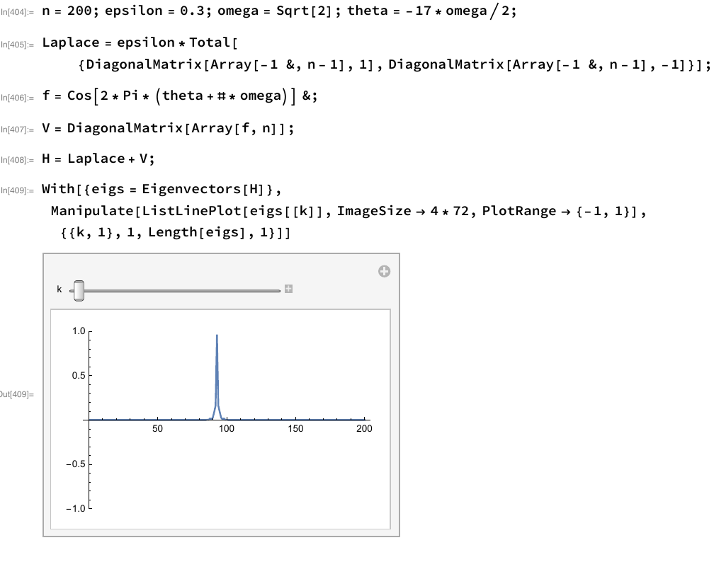
Figure 17. Mathematica code for Figures (9), (10)

References

- [AizMol] Aizenman, M., Molchanov, S. Localization at large disorder and at extreme energies: an elementary derivation. Comm. Math. Phys. 157 (1993), no. 2, 245–278.
- [AizWAr] Aizenman, M., Warzel, S. Random operators. Disorder effects on quantum spectra and dynamics. Graduate Studies in Mathematics, 168. American Mathematical Society, Providence, RI, 2015.
- [Avi] Avila, A. Global theory of one-frequency Schrödinger operators. Acta Math. 215 (2015), no. 1, 1–54.
- [BasPolRoy1] Basu, S., Pollack, R., Roy, M. On the combinatorial and algebraic complexity of quantifier elimination, Journal of the ACM, 43 (1996), no. 6, 1002–1045.
- [BasPolRoy2] Basu, S., Pollack, R., Roy, M. Algorithms in real algebraic geometry, Springer-Verlag, Berlin, 2003.
- [Ber] Berezanskii, J. Expansions in Eigenfunctions of Selfadjoint Operators, Translations of Mathematical Monographs, Vol. 17, Amer. Math. Soc., Providence, R.I., 1968.
- [BouLac] Bougerol, P., Lacroix, J. Products of random matrices with applications to Schrödinger operators. Progress in Probability and Statistics, 8. Birkhäuser Boston, Inc., Boston, MA, 1985.
- [Bou1] Bourgain, J. Green’s function estimates for lattice Schrödinger operators and applications. Annals of Mathematics Studies, 158. Princeton University Press, Princeton, NJ, 2005.
- [Bou2] Bourgain, J. Anderson localization for quasi-periodic lattice Schrödinger operators on , arbitrary. Geom. Funct. Anal. 17 (2007), no. 3, 682–706.
- [BouGol] Bourgain, J.; Goldstein, M. On nonperturbative localization with quasi-periodic potential. Ann. of Math. (2) 152 (2000), no. 3, 835–879.
- [BouGolSch1] Bourgain, J., Goldstein, M., Schlag, W. Anderson localization for Schrödinger operators on with potentials given by the skew-shift. Comm. Math. Phys. 220 (2001), no. 3, 583–621.
- [BouGolSch2] Bourgain, J., Goldstein, M., Schlag, W. Anderson localization for Schrödinger operators on with quasi-periodic potential. Acta Math. 188 (2002), no. 1, 41–86.
- [BDFGVWZ] Bucaj, V., Damanik, D., Fillman, J., Gerbuz, V., VandenBoom, T., Wang, F., Zhang, Z. Localization for the one-dimensional Anderson model via positivity and large deviations for the Lyapunov exponent. Trans. Amer. Math. Soc. 372 (2019), no. 5, 3619–3667.
- [CarKleMar] Carmona, R., Klein, A., Martinelli, F. Anderson localization for Bernoulli and other singular potentials. Comm. Math. Phys. 108 (1987), no. 1, 41–66.
- [CarLac] Carmona, R., Lacroix, J. Spectral theory of random Schrödinger operators. Probability and its Applications. Birkhäuser Boston, Inc., Boston, MA, 1990.
- [CraSim] Craig, W., Simon, B. Subharmonicity of the Lyaponov index. Duke Math. J. 50 (1983), no. 2, 551–560.
- [DamFil1] Damanik, D., Fillman, J. One-Dimensional Ergodic Schrödinger Operators I. General Theory, Graduate Studies in Mathematics, AMS, to appear.
- [DamFil2] Damanik, D., Fillman, J. One-Dimensional Ergodic Schrödinger Operators II. Special Cases, Graduate Studies in Mathematics, AMS, to appear.
- [DinSma] Ding, J., Smart, C. Localization near the edge for the Anderson Bernoulli model on the two dimensional lattice. Invent. Math. 219 (2020), no. 2, 467–506.
- [Far] Faris, W. Perturbations and non-normalizable Eigenvectors, Helvetica Physica Acta, 44 (1971), 930–936.
- [FigPas] Figotin, A., Pastur, L. Spectra of Random and Almost-Periodic Operators, Springer, 1992.
- [ForVan] Forman, Y., VandenBoom, T. Localization and Cantor spectrum for quasiperiodic discrete Schrödinger operators with asymmetric, smooth, cosine-like sampling functions, preprint 2021.
- [FroSpe] Fröhlich, J., Spencer, T. Absence of diffusion in the Anderson tight binding model for large disorder or low energy. Comm. Math. Phys. 88 (1983), no. 2, 151–184.
- [FroSpeWit] Fröhlich, J., Spencer, T., Wittwer, P. Localization for a class of one-dimensional quasi-periodic Schrödinger operators. Comm. Math. Phys. 132 (1990), no. 1, 5–25.
- [FurKes] Fürstenberg, H., Kesten, H. Products of random matrices. Ann. Math. Statist 31 (1960), 457–469.
- [GerKle] Germinet, F., Klein, A. Bootstrap multiscale analysis and localization in random media. Comm. Math. Phys. 222 (2001), no. 2, 415–448.
- [GolSch1] Goldstein, M., Schlag, W. Hölder continuity of the integrated density of states for quasi-periodic Schrödinger equations and averages of shifts of subharmonic functions. Ann. of Math. (2) 154 (2001), no. 1, 155–203.
- [GolSch2] Goldstein, M., Schlag, W. Fine properties of the integrated density of states and a quantitative separation property of the Dirichlet eigenvalues, Geom. Funct. Anal. 18 (2008), no. 3, 755–869.
- [GolSch3] Goldstein, M., Schlag, W. On Schrödinger operators with dynamically defined potentials. Mosc. Math. J. 5 (2005), no. 3, 577–612.
- [GolSchVod] Goldstein, M., Schlag, W., Voda, M. On localization and the spectrum of multi-frequency quasi-periodic operators, https://arxiv.org/abs/1610.00380
- [GorKle] Gorodetski, A., Kleptsyn, V. Parametric Fürstenberg theorem on random products of matrices. Adv. Math. 378 (2021), 107522.
- [HanLemSch] Han, R., Lemm, M., Schlag, W. Effective multi-scale approach to the Schrödinger cocycle over a skew shift base, to appear in Ergodic Theory and Dyn. Systems, preprint 2018.
- [Her] Herman, M. Une méthode pour minorer les exposants de Lyapounov et quelques exemples montrant le charactère local d’un theoreme d’Arnold et de Moser sur le tore de dimension . Comment. Math. Helv. 58 (1983), no. 3, 453–502.
- [Hun] Hundertmark, D. A short introduction to Anderson localization. In: Analysis and stochastics of growth processes and interface models, 194–218, Oxford Univ. Press, Oxford, 2008.
- [Jit] Jitomirskaya, S. Ya. Metal-insulator transition for the almost Mathieu operator. Ann. of Math. (2) 150 (1999), no. 3, 1159–1175.
- [JitMar] Jitomirskaya, S., Marx, C. A. Dynamics and spectral theory of quasi-periodic Schrödinger-type operators. Ergodic Theory Dynam. Systems 37 (2017), no. 8, 2353–2393.
- [JitSim] Jitomirskaya. S., Simon, B. Operators with singular continuous spectrum. III. Almost periodic Schrödinger operators. Comm. Math. Phys., Volume 165, Number 1 (1994), 201–205.
- [JitZhu] Jitomirskaya, S., Zhu, X. Large deviations of the Lyapunov exponent and localization for the 1D Anderson model. Comm. Math. Phys. 370 (2019), no. 1, 311–324.
- [Joh] John, F. Partial differential equations. Reprint of the fourth edition. Applied Mathematical Sciences, 1. Springer-Verlag, New York, 1991.
- [Kir] Kirsch, W. Random Schrödinger operators a course, In: Holden H., Jensen A. (eds) Schrödinger Operators. Lecture Notes in Physics, vol 345. Springer, Berlin, Heidelberg, 1989.
- [Kuc] Kuchment, P. An overview of periodic elliptic operators. Bull. Amer. Math. Soc. 53 (2016), no. 3, 343–414.
- [Lev] Levin, B. Ya. Lectures on entire functions. Translations of Mathematical Monographs, 150. American Mathematical Society, Providence, RI, 1996
- [MagWin] Magnus, W., Winkler, S. Hill’s equation. Corrected reprint of the 1966 edition. Dover Publications, Inc., New York, 1979.
- [Sch] Schlag, W. On the Integrated Density of States for Schrödinger Operators on with Quasi Periodic Potential, Comm. Math. Phys. 223, 47–65 (2001).
- [Sim] Simon, B. Schrödinger semigroups, Bulletin AMS, Vol. 7, No. 3, 1982.
- [SimWol] Simon, B., Wolff, T. Singular continuous spectrum under rank one perturbations and localization for random Hamiltonians. Comm. Pure Appl. Math. 39 (1986), no. 1, 75–90.
- [Sto] Stollmann, P. Wegner estimates and localization for continuum Anderson models with some singular distributions. Archiv der Mathematik volume 75, 307–311, 2000
- [Via] Viana, M. Lectures on Lyapunov exponents. Cambridge Studies in Advanced Mathematics, 145. Cambridge University Press, Cambridge, 2014.
- [vDrKle] von Dreifus, H., Klein, A. A new proof of localization in the Anderson tight binding model. Comm. Math. Phys. 124 (1989), no. 2, 285–299.
- [Weg] Wegner, F. The density of states for disordered systems, Z. Phys. B44 (1981), 9–15.