The Wasserstein space of stochastic processes

Abstract.

Wasserstein distance induces a natural Riemannian structure for the probabilities on the Euclidean space. This insight of classical transport theory is fundamental for tremendous applications in various fields of pure and applied mathematics.

We believe that an appropriate probabilistic variant, the adapted Wasserstein distance $\mathcal{A}\mathcal{W}$, can play a similar role for the class $\mathrm{FP}$ of filtered processes, i.e. stochastic processes together with a filtration. In contrast to other topologies for stochastic processes, probabilistic operations such as the Doob-decomposition, optimal stopping and stochastic control are continuous w.r.t. $\mathcal{A}\mathcal{W}$. We also show that $(\mathrm{FP},\mathcal{A}\mathcal{W})$ is a geodesic space, isometric to a classical Wasserstein space, and that martingales form a closed geodesically convex subspace.

1. Overview

It is often useful to change the view from considering objects in isolation to studying the space of these objects and specifically their mutual relationship w.r.t. the ambient space. A classic instance is to switch from studying functions to considering the Lebesgue- or Sobolev-spaces of functions in functional analysis; a more contemporary example is the passing from measures to the manifold of measures based on optimal transport theory. The aim of this article is to investigate what should be the appropriate ambient space for the class of stochastic processes.

1.1. The space of laws on ${\mathbb{R}}^{N}$ and its limitations

A natural starting point for this is to represent stochastic processes on the canonical probability space. Specifically, the class of real valued processes in finite discrete time $\{1,\ldots,N\}$ is naturally represented as the set ${\mathcal{P}}({\mathbb{R}}^{N})$ of probability measures on ${\mathbb{R}}^{N}$. Importantly, the usual weak topology on ${\mathcal{P}}({\mathbb{R}}^{N})$ fails to capture the temporal structure of stochastic processes and is not strong enough to guarantee continuity of stochastic optimization problems or basic operations like the Doob-decomposition.

As a remedy, a number of researchers from different scientific communities have introduced topological structures on the set of stochastic processes with the common goal to adequately capture the temporal structure. We list Aldous extended weak topology [9] (stochastic analysis), Hellwig’s information topology [57, 58] (economics), Bion-Nadal and Talay’s version of the Wasserstein distance [35] (stochastic analysis, optimal control), Pflug and Pichler’s nested distance [80, 81] (stochastic optimization), Rüschendorf’s Markov constructions [89] (optimal transport), Lassalle’s causal transport problem [72] (optimal transport), and Nielsen and Sun’s chain rule transport [77] (machine learning). Remarkably, in finite discrete time, these seemingly independent approaches define the same topology on ${\mathcal{P}}({\mathbb{R}}^{N})$, the weak adapted topology, see [12].

A natural compatible metric for the weak adapted topology is the adapted Wasserstein distance

$$\mathcal{AW}_{p}^{p}(\mu,\nu)=\inf_{\pi\in\mathrm{Cpl}_{\mathrm{bc}}(\mu,\nu)}{\mathbb{E}}_{\pi}[\|X-Y\|_{p}^{p}],\quad p\in[1,\infty).$$

The difference to the classical Wasserstein distance comes from the fact that one considers only bicausal couplings $\mathrm{Cpl}_{\mathrm{bc}}(\mu,\nu)$, see Definition 2.1 below. These couplings are non-anticipative and can be viewed as a Kantorovich analogue of non-anticipative transport maps, see [34].

While the weak adapted topology / $\mathcal{AW}_{p}$ appear canonical and have recently seen a burst of applications (see [43, 82, 83, 52, 11, 3, 95, 85, 69, 76, 87, 86, 96, 13, 64] among others) we also highlight two limitations:

1. The metric space $({\mathcal{P}}_{p}({\mathbb{R}}^{N}),\mathcal{AW}_{p})$ is not complete. In fact, this shortcoming also arises for other natural distances that respect the information structure of stochastic processes.

2. Following the classical theory of stochastic analysis one would like to consider processes together with a general filtration, not just the filtration generated by the process itself.

1.2. Filtered processes as the completion of $\mathcal{P}_{p}(\mathbb{R}^{N})$

Rather conveniently, these supposed shortcomings already represent their mutual resolution: a possible interpretation of the incompleteness of $({\mathcal{P}}_{p}({\mathbb{R}}^{N}),\mathcal{AW}_{p})$ is that the space ${\mathcal{P}}_{p}({\mathbb{R}}^{N})$ is not ‘large’ enough to represent all processes one would like to consider. In our first main result we show that the extra information that can be stored in an ambient filtration is precisely what is needed to arrive at the completion of $({\mathcal{P}}_{p}({\mathbb{R}}^{N}),\mathcal{AW}_{p})$. To make this precise we need the following definition:

Definition 1.1.

A five-tuple

(1.1) $${\mathbb{X}}:=\big{(}\Omega,\mathcal{F},{\mathbb{P}},(\mathcal{F}_{t})_{t=1}^{N},(X_{t})_{t=1}^{N}\big{)},$$

where $(X_{t})_{t=1}^{N}$ is adapted to $(\mathcal{F}_{t})_{t=1}^{N}$, is called a filtered (stochastic) process. We write $\mathcal{FP}$ for the class of all filtered processes and $\mathcal{FP}_{p}$ for the subclass of processes with ${\mathbb{E}}[\|X\|_{p}^{p}]<\infty$.

Clearly, $\mathcal{P}_{p}({\mathbb{R}}^{N})$ is embedded in $\mathcal{FP}_{p}$: for $\mu\in\mathcal{P}({\mathbb{R}}^{N})$ set ${\mathbb{X}}:=({\mathbb{R}}^{N},\mathcal{B}({\mathbb{R}}^{N}),\mu,(\mathcal{F}_{t})_{t=1}^{N},(X_{t})_{t=1}^{N})$, where $(X_{t})_{t=1}^{N}$ is the canonical process, i.e. $X_{t}(\omega)=\omega(t)$, and $\mathcal{F}_{t}=\sigma(X_{s}:s\leq t)$ for $t\leq N$.

It is relatively straightforward to extend the concept of bicausal couplings to processes with filtrations (see Definition 2.1 for details) and accordingly the notion of adapted Wasserstein distance extends to filtered processes via

$$\mathcal{AW}_{p}^{p}({\mathbb{X}},{\mathbb{Y}}):=\inf_{\pi\in\mathrm{Cpl}_{\mathrm{bc}}({\mathbb{X}},{\mathbb{Y}})}{\mathbb{E}}_{\pi}[\|X-Y\|_{p}^{p}].$$

As in the case of ${\mathscr{L}}^{p}$ / $L^{p}$ spaces (or similar situations), we identify two filtered processes ${\mathbb{X}},{\mathbb{Y}}$ if $\mathcal{AW}_{p}({\mathbb{X}},{\mathbb{Y}})=0$ and denote the corresponding set of equivalence classes by $\mathrm{FP}_{p}$. Our first main result is:

Theorem 1.2.

$\mathcal{AW}_{p}$ is a metric on $\mathrm{FP}_{p}$ and $(\mathrm{FP}_{p},\mathcal{AW}_{p})$ is the completion of $(\mathcal{P}_{p}({\mathbb{R}}^{N}),\mathcal{AW}_{p})$.

We also show in Theorem 5.4 below that certain simpler classes of processes are dense in $\mathrm{FP}_{p}$, e.g. filtered processes that can be represented on a finite state space $\Omega$ or finite state Markov chains. This seems important in view of numerical applications.

1.3. $\mathrm{FP}_{p}$ as geodesic space

In fact, our proof of Theorem 1.2 reveals more, namely the following result on the metric structure of $(\mathrm{FP}_{p},\mathcal{AW}_{p})$:

Theorem 1.3.

There exists a Polish space $(\mathcal{V},d)$ such that $(\mathrm{FP}_{p},\mathcal{AW}_{p})$ is isometric to the classical Wasserstein space $(\mathcal{P}_{p}(\mathcal{V}),\mathcal{W}_{p}^{(d)})$.

Explicitly, $\mathcal{V}$ is constructed by considering Wasserstein spaces of Wasserstein spaces in an iterated fashion as already considered by Vershik [91]. Theorem 1.3 allows to transfer concepts from optimal transport to the theory of stochastic processes, e.g. it allows to consider displacement interpolation and Wasserstein barycenters of filtered processes and to view $(\mathrm{FP}_{p},\mathcal{AW}_{p})$ as a (formal) Riemannian manifold. Specifically, using the work of Lisini [74] we obtain:

Theorem 1.4.

Assume $p>1$. Then $(\mathrm{FP}_{p},\mathcal{AW}_{p})$ is a geodesic space and the set of martingales forms a closed, geodesically convex subspace.

Famously, McCann introduced the concept of displacement interpolation in his thesis [75], giving a new meaning to the transformation of one probability into another. In analogy, Theorem 1.4 suggests an interpolation between stochastic processes.

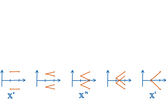
Figure 1. Interpolation between two simple martingales ${\mathbb{X}}^{0}$ and ${\mathbb{X}}^{1}$.

We emphasize that the usual Wasserstein interpolation on $\mathcal{P}_{p}({\mathbb{R}}^{N})$ is not compatible with concepts one would like to consider for stochastic processes, e.g. stochastic optimization problems are not continuous along geodesics, the set of martingales is not displacement convex, etc.

We also note that the set $\mathcal{P}_{p}({\mathbb{R}}^{N})$ is not $\mathcal{AW}_{p}$-displacement convex: even if ${\mathbb{P}},{\mathbb{Q}}\in\mathcal{P}_{p}({\mathbb{R}}^{N})$ are laws of relatively regular processes, the respective geodesic does in general not lie in $\mathcal{P}_{p}({\mathbb{R}}^{N})$, see Example 5.11. This further underlines the importance of considering processes together with their filtration.

1.4. Equivalence of filtered processes

We briefly discuss the equivalence relation induced by

(1.2) $$\mathcal{AW}_{p}({\mathbb{X}},{\mathbb{Y}})=0.$$

Intuitively, one would hope that processes with zero distance are equivalent in the sense that they have identical properties from a probabilistic perspective. In fact, based on formalizing what assertions belong to the ‘language of probability’, Hoover–Keisler [62] have made precise what it should mean that two processes ${\mathbb{X}},{\mathbb{Y}}$ have the same probabilistic properties. ${\mathbb{X}}$ and${\mathbb{Y}}$ are then called equivalent in adapted distribution, in signs ${\mathbb{X}}\sim_{\infty}{\mathbb{Y}}$. We will establish below that equivalence in adapted distribution can be expressed in terms of adapted Wasserstein distance:

Theorem 1.5.

Let ${\mathbb{X}},{\mathbb{Y}}\in\mathcal{FP}_{p}$. Then ${\mathbb{X}}\sim_{\infty}{\mathbb{Y}}$ if and only if $\mathcal{AW}_{p}({\mathbb{X}},{\mathbb{Y}})=0$.

Informally, Theorem 1.5 asserts that the equivalence classes in $\mathrm{FP}_{p}$ collect precisely all representatives of a process that should be considered identical from a probabilist’s point of view.

Other (more familiar) notions of equivalence on $\mathcal{FP}$ are equivalence in law, in symbols $\sim_{0}$, and Aldous’ notion of synonymity, in symbols $\sim_{1}$. Both of these are strictly coarser than $\sim_{\infty}$ and may identify processes that have different probabilistic properties. For example, there are filtered processes ${\mathbb{X}},{\mathbb{Y}}$ with ${\mathbb{X}}\sim_{0}{\mathbb{Y}}$ where ${\mathbb{X}}$ is a martingale while ${\mathbb{Y}}$ is not. Similarly, we will construct examples of processes ${\mathbb{X}},{\mathbb{Y}}$ where ${\mathbb{X}}\sim_{1}{\mathbb{Y}}$ but optimal stopping problems written on ${\mathbb{X}},{\mathbb{Y}}$ lead to different results (see Theorem 7.1).

1.5. Continuity of Doob-decomposition, optimal stopping, Snell-envelope

In line with Theorem 1.5, $\mathcal{AW}_{p}({\mathbb{X}},{\mathbb{Y}})=0$ implies that ${\mathbb{X}}$ and ${\mathbb{Y}}$ have the same Doob-decomposition, that optimal stopping problems of the form

(1.3) $$\sup_{\tau}{\mathbb{E}}[G_{\tau}(X_{1},\ldots,X_{\tau})],$$

where $\tau$ runs through all $(\mathcal{F}_{t})_{t=1}^{N}$-stopping times, yield the same optimal value and have the same Snell-envelop. Moreover, we show that the above operations are continuous w.r.t.  the weak adapted topology, indeed we establish:

Theorem 1.6.

The mapping that assigns to a filtered process its Doob-decomposition is Lipschitz continuous. If $G_{t}\colon{\mathbb{R}}^{t}\to{\mathbb{R}}$ is bounded and continuous (resp.  Lipschitz) for each $t$, then (1.3) is continuous (resp.  Lipschitz) in ${\mathbb{X}}$.

In Section 6 we collect further statements of similar flavour as Theorem 1.6. It is important to note that comparable results do not hold w.r.t. to other (coarser) topologies for filtered processes. Specifically, convergence in Aldous’ extended weak topology is strictly weaker than convergence in $\mathcal{AW}_{p}$ and is not strong enough to obtain continuity of optimal stopping problems (see Section 7). This seems remarkable, since Aldous [9, page 105] deliberates the question which framework is natural to study continuity of optimal stopping.

1.6. Canonical representatives of filtered processes

A slightly altered variant $\mathcal{Z}$ of the Polish space $\mathcal{V}$ appearing in Theorem 1.3 also plays an important role in finding canonical representatives for the equivalence classes in $\mathrm{FP}$: In Section 3 below we will show that there exists $(\mathcal{Z},\mathcal{F}^{\mathcal{Z}},(\mathcal{F}_{t}^{\mathcal{Z}})_{t=1}^{N},(Z_{t})_{t=1}^{N})$ with $\mathcal{Z}$ Polish, such that every filtered process ${\mathbb{X}}$ is represented in a canonical way via a probability on $\mathcal{Z}$, i.e. there exists ${\mathbb{Q}}^{{\mathbb{X}}}\in{\mathcal{P}}(\mathcal{Z})$ such that

$$(\mathcal{Z},\mathcal{F}^{\mathcal{Z}},{\mathbb{Q}}^{{\mathbb{X}}},(\mathcal{F}_{t}^{\mathcal{Z}})_{t=1}^{N},(Z_{t})_{t=1}^{N})\sim_{\infty}{\mathbb{X}}.$$

In particular, all information about the process ${\mathbb{X}}$ is stored in the corresponding measure ${\mathbb{Q}}^{{\mathbb{X}}}$, while the underlying probability space $\Omega$, the representing stochastic process $Z$ and the respective filtration do not depend on ${\mathbb{X}}$. In this sense the situation is analogous to the canonical representation of stochastic processes via probabilities on the path space. In view of Theorem 1.5 this also implies that one can assume without loss of generality that a given filtered process is defined on a Polish probability space.

1.7. Prohorov-type result and barycenter of processes

An extremely useful property of the usual weak topology is the abundance of (pre-)compact sets based on Prohorov’s theorem. Remarkably, this carries over to ‘adapted’ topologies. This was first established by Hoover [60, Theorem 4.3], see also [11, Lemma 1.7]. In the present context this fact can be expressed as follows:

Theorem 1.7.

A set $K\subseteq\mathrm{FP}_{p}$ is $\mathcal{AW}_{p}$-precompact if and only if the respective set of laws in $\mathcal{P}_{p}(\mathbb{R}^{N})$ is $\mathcal{W}_{p}$-precompact.

Note that by Prohorov’s theorem, $\mathcal{W}_{p}$-precompactness in $\mathcal{P}_{p}({\mathbb{R}}^{N})$ is equivalent to tightness plus uniform $p$-integrability, see for instance [94].

Theorem 1.7 is relevant in several proofs given below and has important consequences for the applications of our results presented in Section 6. For instance, it allows us to establish the existence of barycenters of stochastic processes: Famously, Agueh and Carlier [6] introduced the concept of barycenters w.r.t. Wasserstein distance which has striking consequences in machine learning (e.g. [88, 42]), statistics (e.g. [78, 18]) as well as in pure mathematics (e.g. [73, 68]). In Theorem 6.7 we show that for filtered processes ${\mathbb{X}}^{1},\ldots,{\mathbb{X}}^{k}\in\mathrm{FP}_{p}$ and convex weights $\lambda_{1},\ldots,\lambda_{k}$ there exists a barycenter process i.e. a filtered process ${\mathbb{X}}^{*}\in\mathrm{FP}_{p}$ which minimizes

$$\inf_{{\mathbb{X}}}\lambda_{1}\mathcal{A}\mathcal{W}_{p}^{p}({\mathbb{X}}^{1},{\mathbb{X}})+\ldots+\lambda_{k}\mathcal{A}\mathcal{W}_{p}^{p}({\mathbb{X}}^{k},{\mathbb{X}}).$$

1.8. Applications and extensions

As already noted above, the adapted Wasserstein distance improves over the classical weak topology / Wasserstein distance in that it guarantees stability of basic operations such as the Doob-decomposition and optimal stopping. Naturally we expect similar results for other probabilistic problems with inherent time structure. In this line, we describe applications to stability of stochastic optimal control, utility maximization and pricing / hedging, robust finance in the realm of American options, conditional McKean-Vlasov control, and weak optimal transport, see Sections 6.1 - 6.8 below. In view of applications it is relevant that adapted Wasserstein distance can be efficiently computed numerically as well as estimated from given data; we comment on this in Section 6.9.

While the focus of the present article lies on stochastic processes in finite discrete time, extensions to more general cases are intriguing. In Appendix B we consider the case of infinite discrete time, i.e. the set $\mathrm{FP}^{(\infty)}$ of processes $(X_{t})_{t=1}^{\infty}$ whose paths lie in ${\mathbb{R}}^{\infty}$ (or a countable product of Polish spaces). We obtain results very similar to the finite discrete time case, mainly based on limiting arguments. A notable difference is that the path space ${\mathbb{R}}^{\infty}$ is not geodesic and hence $\mathrm{FP}^{(\infty)}$ is not geodesic either.

Concerning continuous time processes $(X_{t})_{t\in[0,T]}$, it is known from stochastic analysis, that different applications require the use of different topologies / metrics on the path space. This fact appears even more noticeable when also information is taken into account. In Appendix C we briefly present adapted topologies for continuous time stochastic processes that have been used in the literature or seem sensible. We describe how $\mathcal{AW}$ needs to be altered to fit the respective choices and comment on some strengths and weaknesses of the emerging theories.

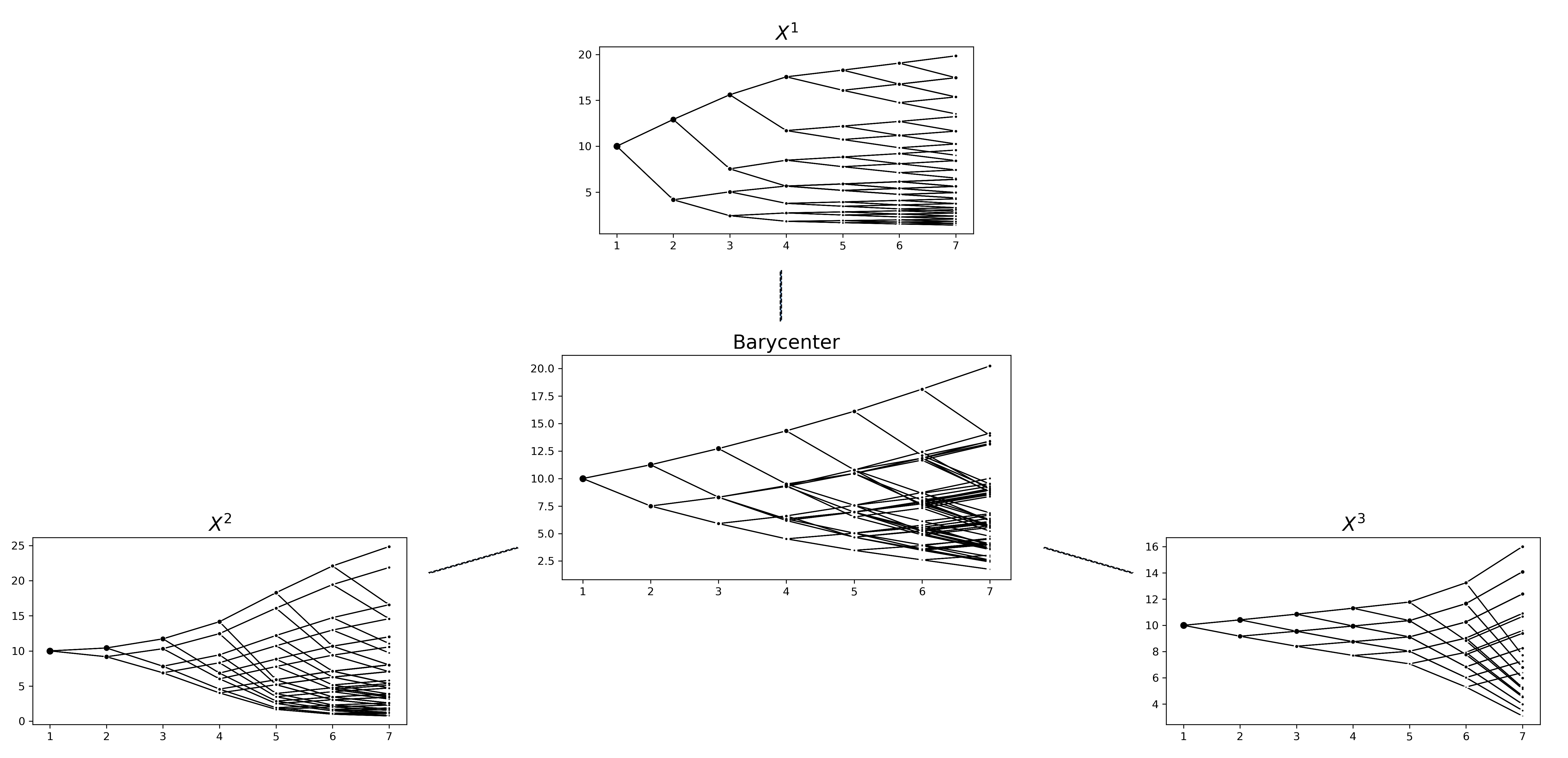
Figure 2. Three CRR-type models as considered in finance and econometrics and their barycenter (implemented by Stephan Eckstein).

1.9. Remarks on related literature.

Imposing a ‘causality’ constraint on a transport plan between laws of processes seems to go back to the Yamada–Watanabe criterion for stochastic differential equations [99] and is used under the name ‘compatibility’ by Kurtz [71].

A systematic treatment and use of causality as an interesting property of abstract transport plans between filtered probability spaces and their associated optimal transport problems was initiated by Lassalle [72] and Acciaio, Backhoff, and Zalashko [2].

As noted above, different groups of authors have introduced similar ‘adapted’ variants of the Wasserstein distance, this includes the works of Vershik [91, 92], Rüschendorf [89], Gigli [51, Chapter 4] (see also [10, Section 12.4]), Pflug and Pichler [80], Bion-Nadal and Talay [35], and Nielsen and Sun [77]. Pflug and Pichler’s nested distance has had particular impact in multistage programming, see [81, 82, 52, 69, 86] among others.

In addition to these distances, extensions of the weak topology that account for the flow of information were introduced by Aldous in stochastic analysis [9] (based on Knight’s prediction process [70]), Hoover and Keisler in mathematical logic [62, 60] and Hellwig in economics [57]. Very recently, an approach using higher rank signatures was given by Bonner, Liu, and Oberhauser [36], in particular providing a metric for convergence in adapted distribution in the sense of Hoover–Keisler.

The idea to represent information (in the sense of filtrations) using conditional distributions originated in the theory of dynamical systems and Vershik’s program to classify filtrations whose time horizons starts at $-\infty$, see e.g. [92] and in particular the survey [93]. For a more probabilistic account of this line of research we refer to [47]. Independently, Pflug [79] introduced this idea in stochastic optimization and defined the space of ‘nested distributions’.

Recently, there has been significant interest in adapted / causal transport problems in discrete time or with a finite number of hierarchical levels. A goal of the present article is to provide the theoretical framework for these emerging lines of research and we briefly indicate some of these directions: In mathematical finance, the use of weak adapted topologies was initiated in the context of game options [43]. Further contributions apply adapted transport and adapted Wasserstein distances to questions of insider trading and enlargement of filtrations [2], stability of pricing / hedging and utility maximization [52, 22, 23, 11, 1, 30, 31] and interest rate uncertainty [3]. Adapted transport is used in [21] to study the sensitivity of multiperiod optimization problems and distributionally robust optimization problems. In [56] it is applied to time-dynamic matching problems [24], and in [90, 63] for the computational resolution of optimal stopping and other filtration-dependent problems. In [38] a connection of adapted transport to the Weisfeiler-Lehman distance is reveiled. Machine learning algorithms based on adapted or hierarchical structures are studied in the context of image processing [65], text processing and hierarchical domain translation [100, 46], causal graph learning [7], video prediction and generation [98, 97], and universal approximation [5]. In [39], adapted transport is used as the starting point to develop a framework for more general causal dependence structures.

1.10. Organization of the paper

In Section 2 we introduce some important concepts and in particular the notions of (bi-) causality and adapted Wasserstein distance.

In Section 3 we formally discuss the Wasserstein space of filtered processes $\mathrm{FP}_{p}$ as a preparation to establish Theorem 1.2 and Theorem 1.3 subsequently. In Subsection 3.1 we construct a canonical filtered space that supports for each equivalence class ${\mathbb{X}}\in\mathrm{FP}_{p}$ a canonical representative. Building on the foregoing subsections, we establish in Subsection 3.2 an isometric isomorphism between filtered processes, their canonical counterparts, and a classical Wasserstein space.

Section 4 links the weak adapted topology to the concept of adapted functions and the prediction process by Hoover and Keisler.

Section 5 deals with topological and geometric aspects. We prove a compactness criterion, show that $\mathrm{FP}_{p}$ is the completion of $\mathcal{P}_{p}({\mathbb{R}}^{N})$ and prove that finite state Markov processes are dense in $\mathrm{FP}_{p}$, prove that $\mathrm{FP}_{p}$ is a geodesic space for $1<p<\infty$, and show that martingales form a closed, geodesically convex subset of $\mathrm{FP}_{p}$.

In Section 6 we discuss applications and comment on numerical aspects related to $\mathcal{AW}$.

Section 7 is concerned with an example that, among other things, shows that Aldous’ extended weak topology fails to guarantee continuity of optimal stopping problems.

Finally, in Appendix A, we discuss a notion of ‘block approximation’ of couplings, which is an auxiliary concept required to prove the results in Subsection 3.2 for probability spaces that are not necessarily Polish. In Appendix B and C we discuss extensions of the present setting to the case of stochastic processes index by infinite discrete time and continuous time, respectively.

2. Notational conventions

Throughout this article, we fix a time horizon $N\in\mathbb{N}$ and $1\leq p<\infty$. For each time $1\leq t\leq N$, let $\mathcal{X}_{t}$ be a Polish space with a fixed compatible complete metric $d_{\mathcal{X}_{t}}$. If $\mathcal{X}_{t}={\mathbb{R}}^{d}$, then $d_{t}(x,y)=|x-y|$ where $|\cdot|=\|\cdot\|_{2}$ is the Euclidean norm. Given a finite family of sets $(A_{u})_{u=1}^{t}$ and $1\leq s\leq t$, we use the following abbreviation for its product

$$A_{s:t}:=A_{s}\times\ldots\times A_{t}.$$

The same convention applies to vectors. For $s\leq r\leq t$, the projection onto the $r$-th coordinate of $A_{s:t}$ is denoted by $\mathrm{pj}_{r}\colon A_{s:t}\to A_{r}$. Using this convention we are interested in stochastic processes taking values in the path space $\mathcal{X}:=\mathcal{X}_{1:N}$. Processes on $\mathcal{X}$ are usually denoted by capital letters, i.e., $X=(X_{t})_{t=1}^{N}$, whereas specific elements of the path space are denoted by lower case, i.e., $(x_{t})_{t=1}^{N}\in\mathcal{X}_{1:N}$.

Distances: For a Polish space $\mathcal{A}$ with fixed compatible complete metric $d_{\mathcal{A}}$, we write $\mathcal{P}(\mathcal{A})$ for the set of Borel probability measures on $\mathcal{A}$, and $\mathcal{P}_{p}(\mathcal{A})$ for the subset whose elements integrate $d^{p}_{\mathcal{A}}(\cdot,a_{0})$ for some (and hence all) $a_{0}\in\mathcal{A}$. If $\mathcal{B}$ is another Polish space and $\mu\in\mathcal{P}(\mathcal{A})$, $\nu\in\mathcal{P}(\mathcal{B})$, we write $\mathrm{Cpl}(\mu,\nu)$ for the set of all couplings with marginals $\mu,\nu$, that is $\pi\in\mathrm{Cpl}(\mu,\nu)$ if $\pi\in\mathcal{P}(\mathcal{A}\times\mathcal{B})$ and its first marginal equals $\mu$ and its second $\nu$. We equip $\mathcal{P}(\mathcal{A})$ with the topology of weak convergence and $\mathcal{P}_{p}(\mathcal{A})$ with the ($p$-th order) Wasserstein distance $\mathcal{W}_{\mathcal{P}_{p}(\mathcal{A})}$, that is

$$\mathcal{W}_{\mathcal{P}_{p}(\mathcal{A})}^{p}(\mu,\nu):=\inf_{\pi\in\mathrm{Cpl}(\mu,\nu)}\int d_{\mathcal{A}}^{p}(a,\hat{a})\,\pi(da,d\hat{a}).$$

This renders $\mathcal{P}(\mathcal{A})$ and $\mathcal{P}_{p}(\mathcal{A})$ Polish spaces. Note that for a bounded metric, the weak convergence topology and the one induced by $\mathcal{W}_{p}$ coincide. Whenever clear from context, we will omit excessive subscripts and simply write $d$ and $\mathcal{W}_{p}$ for $d_{\mathcal{A}}$ and $\mathcal{W}_{\mathcal{P}_{p}(\mathcal{A})}$ respectively.

Filtrations: For a filtered process ${{\mathbb{X}}}=(\Omega^{{\mathbb{X}}},\mathcal{F}^{{\mathbb{X}}},{\mathbb{P}}^{{\mathbb{X}}},(\mathcal{F}^{{\mathbb{X}}}_{t})_{t=1}^{N},(X_{t})_{t=1}^{N})$, we use the convention that $\mathcal{F}^{{\mathbb{X}}}_{0}:=\{\emptyset,\Omega^{{\mathbb{X}}}\}$. It is important to note that since the processes start at time $t=1$, this convention is only notational and does not imply that the initial $\sigma$-algebra is trivial. Frequently we consider multiple products of $\sigma$-algebras. To prevent notation getting out of hand, we write

$$\mathcal{F}_{t,s}^{{\mathbb{X}},{\mathbb{Y}}}:=\mathcal{F}_{t}^{\mathbb{X}}\otimes\mathcal{F}_{s}^{\mathbb{Y}}\quad\text{for }0\leq s,t\leq N$$

for two filtered processes ${\mathbb{X}}$ and ${\mathbb{Y}}$. Moreover, we will often identify $\mathcal{F}^{{\mathbb{X}},{\mathbb{Y}}}_{0,t}$ with $\mathcal{F}^{{\mathbb{Y}}}_{t}$; e.g. an $\mathcal{F}^{{\mathbb{X}},{\mathbb{Y}}}_{0,t}$-measurable functions is naturally associated on $\Omega^{{\mathbb{X}}}\times\Omega^{{\mathbb{Y}}}$ with an $\mathcal{F}^{{\mathbb{Y}}}_{t}$-measurable function depending only on the second coordinate, and vice versa. In a similar manner, for a function $f\colon A_{t}\to\mathcal{Y}$, we continue to write $f\colon A_{1:n}\to\mathcal{Y}$ for the function $f\circ\mathrm{pr}_{t}$.

Couplings: In optimal transport couplings are the central tool for comparing probability measures. For filtered processes this role is taken by bicausal couplings, i.e. couplings which respect the information structure of the underlying filtered probability spaces.

Definition 2.1 (Causal couplings).

Let ${\mathbb{X}}$, ${\mathbb{Y}}$ be filtered processes. A probability $\pi$ on $(\Omega^{\mathbb{X}}\times\Omega^{\mathbb{Y}},\mathcal{F}^{\mathbb{X}}\otimes\mathcal{F}^{\mathbb{Y}})$ is called coupling between ${\mathbb{X}}$ and ${\mathbb{Y}}$ if its marginals are ${\mathbb{P}}^{\mathbb{X}}$ and ${\mathbb{P}}^{\mathbb{Y}}$. We call $\pi$

1. causal (or causal from ${\mathbb{X}}$ to ${\mathbb{Y}}$) if, for every $1\leq t\leq N$, conditionally on $\mathcal{F}^{{\mathbb{X}},{\mathbb{Y}}}_{t,0}$ we have that $\mathcal{F}^{{\mathbb{X}},{\mathbb{Y}}}_{N,0}$ and $\mathcal{F}^{{\mathbb{X}},{\mathbb{Y}}}_{0,t}$ are independent,

2. anticausal (or causal from ${\mathbb{Y}}$ to ${\mathbb{X}}$) if, for every $1\leq t\leq N$, conditionally on $\mathcal{F}^{{\mathbb{X}},{\mathbb{Y}}}_{0,t}$ we have that $\mathcal{F}^{{\mathbb{X}},{\mathbb{Y}}}_{0,N}$ and $\mathcal{F}^{{\mathbb{X}},{\mathbb{Y}}}_{t,0}$ are independent,

3. bicausal if it is both, causal and anticausal.

We write $\mathrm{Cpl}({\mathbb{X}},{\mathbb{Y}})$, $\mathrm{Cpl}_{\mathrm{c}}({\mathbb{X}},{\mathbb{Y}})$ and $\mathrm{Cpl}_{\mathrm{bc}}({\mathbb{X}},{\mathbb{Y}})$ for the set of couplings, causal couplings, and bicausal couplings, respectively.

In case that the underlying spaces are path spaces equipped with canonical filtration / processes, these definitions correspond precisely to the classical definitions given in the literature, see [80, 81, 16, 14, 12] among others. In the context of space with more general filtrations causality and causal transport are considered in [72, 2].

The following lemma provides useful characterizations of causality which we will frequently use throughout the article.

Lemma 2.2 (Causality).

Let $\pi$ be a coupling between two filtered processes ${\mathbb{X}}$ and ${\mathbb{Y}}$. Then the following are equivalent.

1. $\pi$ is causal (from ${\mathbb{X}}$ to ${\mathbb{Y}}$).

2. ${\mathbb{E}}_{\pi}[U|\mathcal{F}^{{\mathbb{X}},{\mathbb{Y}}}_{t,t}]={\mathbb{E}}_{\pi}[U|\mathcal{F}^{{\mathbb{X}},{\mathbb{Y}}}_{t,0}]$ for all $1\leq t\leq N$ and bounded $\mathcal{F}_{N}^{\mathbb{X}}$-mb. $U$.

3. ${\mathbb{E}}_{\pi}[V|\mathcal{F}^{{\mathbb{X}},{\mathbb{Y}}}_{N,0}]={\mathbb{E}}_{\pi}[V|\mathcal{F}^{{\mathbb{X}},{\mathbb{Y}}}_{t,0}]$ for all $1\leq t\leq N$ and bounded $\mathcal{F}_{t}^{\mathbb{Y}}$-mb. $V$.

Moreover, $U$ in (ii) can be allowed to be $\mathcal{F}^{{\mathbb{X}},{\mathbb{Y}}}_{t,N}$-measurable and $V$ in (iii) can be allowed to be $\mathcal{F}^{{\mathbb{X}},{\mathbb{Y}}}_{t,t}$-measurable.

In words, (ii) says that given the past of ${\mathbb{X}}$, the past of ${\mathbb{Y}}$ does not provide additional information about the future of ${\mathbb{X}}$ and (iii) says that given the past of ${\mathbb{X}}$, the future of ${\mathbb{X}}$ does not provide additional information about the past of ${\mathbb{Y}}$.

Proof of Lemma 2.2.

The equivalence between (i)-(iii) is a consequence of [66, Proposition 5.6]. The second statement follows from a standard application of the monotone class theorem. ∎

The adapted Wasserstein distance between filtered processes ${\mathbb{X}}$ and ${\mathbb{Y}}$ taking values in $\mathcal{X}$ is then defined as

$$\mathcal{A}\mathcal{W}_{p}^{p}({\mathbb{X}},{\mathbb{Y}}):=\inf_{\pi\in\mathrm{Cpl}_{\mathrm{bc}}({\mathbb{X}},{\mathbb{Y}})}{\mathbb{E}}_{\pi}[d_{\mathcal{X},p}^{p}(X,Y)]\quad\text{where }d_{\mathcal{X},p}(x,y)=\Big{(}\sum_{t=1}^{N}d_{\mathcal{X}_{t}}^{p}(x_{t},y_{t})\Big{)}^{\frac{1}{p}}.$$

When clear from context, we write $d$ instead of $d_{\mathcal{X},p}$. Similarly, we write ${\mathbb{E}}[f(X)]$ instead of ${\mathbb{E}}_{{\mathbb{P}}^{{\mathbb{X}}}}[f(X)]$ etc.

Kernels and product measures: For two Polish spaces $\mathcal{A}$ and $\mathcal{B}$, the term kernel refers to a Borel-measurable mapping $k\colon\mathcal{A}\to\mathcal{P}_{p}(\mathcal{B})$. For $\mu\in\mathcal{P}_{p}(\mathcal{A})$ and a kernel $k$, we write $\mu\otimes k\in\mathcal{P}_{p}(\mathcal{A}\times\mathcal{B})$ for the measure given by $\mu\otimes k(A\times B)=\int_{A}k^{a}(B)\,\mu(da)$. If $\nu\in\mathcal{P}_{b}(\mathcal{B})$ we write $\mu\otimes\nu\in\mathcal{P}_{p}(\mathcal{A}\times\mathcal{B})$ for the product measure. For a measure $\mu\in\mathcal{P}(\mathcal{A})$ and a Borel-measurable mapping $f\colon\mathcal{A}\to\mathcal{B}$, the push-forward of $\mu$ under $f$ is denoted by $f_{\ast}\mu$.

3. The Wasserstein space of stochastic processes

3.1. The canonical filtered space

In order to prove Theorem 1.2 we introduce the canonical space of filtered processes. The classical canonical space of a stochastic process $X$ is the triplet consisting of path space, Borel-$\sigma$-algebra, and its induced law. Clearly, this triplet is adequate if one is interested solely in trajectorial properties of the process. However, the filtration is a major part of filtered processes ${\mathbb{X}}\in\mathcal{FP}$ and therefore we need to capture the information contained in its filtration $\mathcal{F}^{\mathbb{X}}$ in a canonical way. Thus we need to define a canonical space which is capable to carry besides the path properties also the relevant informational properties of ${\mathbb{X}}$.

As an instructional example, consider two 1-step filtered processes ${\mathbb{X}}$ and ${\mathbb{Y}}$ taking values in $\mathcal{X}=\mathcal{X}_{1}\times\mathcal{X}_{2}=\{0\}\times\{-1,1\}$. We write $\mathcal{G}_{1}$ for the trivial $\sigma$-algebra, $\mathcal{G}_{2}=\mathcal{B}$ for the Borel $\sigma$-algebra on $\mathcal{X}$, and $X=(X_{t})_{t=1}^{2}$ for the coordinate process on $\mathcal{X}$. Let ${\mathbb{P}}:=\frac{1}{2}(\delta_{(0,-1)}+\delta_{(0,1)})$, and define

$${\mathbb{X}} :=\left(\mathcal{X},\mathcal{B},{\mathbb{P}},(\mathcal{G}_{1},\mathcal{G}_{2}),X\right)\quad\text{and}\quad{\mathbb{Y}}:=\left(\mathcal{X},\mathcal{B},{\mathbb{P}},(\mathcal{G}_{2},\mathcal{G}_{2}),X\right).$$

Even though the laws of the paths of the two processes coincide, their probabilistic behavior is very different due to their different filtrations, specifically we have

(3.1) $$\mathscr{L}(X_{2}|\mathcal{F}_{1}^{{\mathbb{X}}})(\omega)=\frac{1}{2}(\delta_{-1}+\delta_{1})\text{ whereas }\mathscr{L}(X_{2}|\mathcal{F}_{1}^{{\mathbb{Y}}})(\omega)=\delta_{X_{2}(\omega)}.$$

From this perspective, the product $\mathcal{X}_{1}\times\mathcal{P}(\mathcal{X}_{2})$ is adequate to capture $X_{1}$ and additionally the information on $X_{2}$ we can witness at time 1 based on the filtration, that is $(X_{1},\mathscr{L}(X_{2}|\mathcal{F}_{1}^{{\mathbb{X}}}))$.

This observation leads to the definition of what we baptize the canonical filtered space, the information process, and the canonical filtered process below:

Definition 3.1 (Canonical space).

Fix $p\in[1,\infty)$. We iteratively define a sequence of nested spaces. We write $(\mathcal{Z}_{N},d_{\mathcal{Z}_{N}}):=(\mathcal{X}_{N},d_{\mathcal{X}_{N}})$ and recursively for $t=N-1,\dots,1$

(3.2) $$\mathcal{Z}_{t}:=\mathcal{Z}_{t}^{-}\times\mathcal{Z}_{t}^{+}:=\mathcal{X}_{t}\times\mathcal{P}_{p}(\mathcal{Z}_{t+1})$$

with metric $d_{\mathcal{Z}_{t}}^{p}:=d_{\mathcal{X}_{t}}^{p}+\mathcal{W}_{p,\mathcal{P}(\mathcal{Z}_{t+1})}^{p}$. The elements of $\mathcal{Z}_{t}$ are denoted by $z_{t}=(z_{t}^{-},z_{t}^{+})\in\mathcal{Z}_{t}^{-}\times\mathcal{Z}_{t}^{+}$. The canonical filtered space is given by the triplet

(3.3) $$\left(\mathcal{Z},\mathcal{F}^{\mathcal{Z}},(\mathcal{F}^{\mathcal{Z}}_{t})_{t=1}^{N}\right),$$

where $\mathcal{Z}_{1:N}$ is denoted by $\mathcal{Z}$, elements of $\mathcal{Z}$ by $z=z_{1:N}$, the Borel-$\sigma$-algebra on $\mathcal{Z}$ by $\mathcal{F}^{\mathcal{Z}}$, and $\sigma(z\mapsto z_{1:t})$ by $\mathcal{F}_{t}^{\mathcal{Z}}$. In the context of the canonical filtered space the map $Z^{-}\colon\mathcal{Z}\to\mathcal{X}_{1:N}$ denotes the evaluation map

(3.4) $$Z^{-}(z):=(Z^{-}_{t}(z))_{t=1}^{N}:=(z_{t}^{-})_{t=1}^{N}.$$

The spaces introduced in Definition 3.1 are Polish as all operations involved in their definition preserve this property. The next definition associates to a filtered process ${\mathbb{X}}$ its canonical counterpart – the information process $\mathrm{ip}({\mathbb{X}})$ defined on $\Omega^{{\mathbb{X}}}$ and taking values in $\mathcal{Z}$. We shall later see that the information process selects all information contained in the original filtration relevant for the process; hence its name.

Definition 3.2 (The information process).

To each ${\mathbb{X}}\in\mathcal{FP}$, we associate its information process $\mathrm{ip}({\mathbb{X}})=(\mathrm{ip}_{t}({\mathbb{X}}))_{t=1}^{N}$ defined by setting

$$\mathrm{ip}_{N}({\mathbb{X}})\colon\Omega^{\mathbb{X}} \to\mathcal{Z}_{N},\quad\omega\mapsto X_{N}(\omega)$$

and, recursively for $t=N-1,\dots,1$,

$$\mathrm{ip}_{t}({\mathbb{X}})=(\mathrm{ip}_{t}^{-}({\mathbb{X}}),\mathrm{ip}_{t}^{+}({\mathbb{X}}))\colon\Omega^{\mathbb{X}} \to\mathcal{Z}_{t},\quad\omega\mapsto\left(X_{t}(\omega),\mathscr{L}(\mathrm{ip}_{t+1}({\mathbb{X}})|\mathcal{F}_{t}^{\mathbb{X}})(\omega)\right).$$

Note that $\mathrm{ip}_{t}^{-}({\mathbb{X}})$ is $\mathcal{Z}_{t}^{-}$-valued and $\mathrm{ip}_{t}^{+}({\mathbb{X}})$ is $\mathcal{Z}_{t}^{+}$-valued. In particular this implies that the information process is well-defined: as $(\mathcal{Z}_{t})_{t=1}^{N}$ consists of Polish spaces, the conditional probabilities appearing in the recursive definition of $\mathrm{ip}({\mathbb{X}})$ above exist.

The information processes will be an essential ingredient when we define canonical representatives of filtered processes (see Definition 3.8 below). The next lemma can be seen as a first justification of its name:

Lemma 3.3 (The information process is self-aware).

For every bounded, Borel (continuous) function $f\colon\mathcal{Z}\to{\mathbb{R}}$ and every $1\leq t\leq N$ there is a bounded, Borel (continuous) function $g\colon\mathcal{Z}_{1:t}\to{\mathbb{R}}$ such that

$${\mathbb{E}}[f(\mathrm{ip}({\mathbb{X}}))|\mathcal{F}_{t}^{\mathbb{X}}]=g(\mathrm{ip}_{1:t}({\mathbb{X}}))\quad\text{for all }{\mathbb{X}}\in\mathcal{FP}.$$

More generally, let $\mathcal{A}$ be a Polish space. For every Borel (continuous) function $f\colon\mathcal{Z}\to\mathcal{A}$ and every $1\leq t\leq N$ there is a Borel (continuous) function $g\colon\mathcal{Z}_{1:t}\to\mathcal{P}(\mathcal{A})$ such that

$$\mathscr{L}(f(\mathrm{ip}({\mathbb{X}}))|\mathcal{F}_{t}^{\mathbb{X}})=g(\mathrm{ip}_{1:t}({\mathbb{X}}))\quad\text{for all }{\mathbb{X}}\in\mathcal{FP}.$$

This lemma is an easy consequence of properties of the unfold operator introduced below, see Lemma 3.5. Nevertheless, to boost the reader’s intuition, we want to include a direct proof for the first statement in the notationally lighter case $N=2$:

Sketch of proof for $N=2$.

For $t=2$ there is nothing to do, as $\mathrm{ip}({\mathbb{X}})$ is $\mathcal{F}_{2}^{\mathbb{X}}$-measurable. Let $t=1$. For simplicity, we assume first that $f$ is a product $f(z_{1},z_{2})=f_{1}(z_{1})f_{2}(z_{2})$ for suitable $f_{1}$ and $f_{2}$. Then we can write

$${\mathbb{E}}[f(\mathrm{ip}({\mathbb{X}}))|\mathcal{F}_{1}^{\mathbb{X}}] =f_{1}(\mathrm{ip}_{1}({\mathbb{X}})){\mathbb{E}}[f_{2}(\mathrm{ip}_{2}({\mathbb{X}}))|\mathcal{F}_{1}^{\mathbb{X}}]=f_{1}(\mathrm{ip}_{1}({\mathbb{X}}))\int f_{2}(z_{2})\,\mathscr{L}(\mathrm{ip}_{2}({\mathbb{X}})|\mathcal{F}_{1}^{\mathbb{X}})(dz_{2}),$$

where we used that $\mathrm{ip}_{1}({\mathbb{X}})$ is $\mathcal{F}_{1}^{\mathbb{X}}$-measurable. By definition $\mathrm{ip}_{1}^{+}({\mathbb{X}})=\mathscr{L}(\mathrm{ip}_{2}({\mathbb{X}})|\mathcal{F}_{1}^{\mathbb{X}})$, whence

$${\mathbb{E}}[f(\mathrm{ip}({\mathbb{X}}))|\mathcal{F}_{1}^{\mathbb{X}}] =g(\mathrm{ip}_{1}({\mathbb{X}}))\quad\text{for }\quad g(z_{1}):=f_{1}(z_{1})\int f_{2}(z_{2})\,z_{1}^{+}(dz_{2}).$$

For general $f$ not necessarily of product form, a straightforward application of the monotone class theorem concludes the proof. ∎

In what follows, we are often dealing with mappings between nested spaces of probability measures with different algebraic structures. The unfold operator, introduced below, is an essential tool in reducing bookkeeping to a comprehensible level.

Definition 3.4 (Unfold).

For every $1\leq t\leq N-1$, we define

(3.5) $$\begin{split}\mathrm{uf}_{t}&\colon\mathcal{P}_{p}(\mathcal{Z}_{t})\to\mathcal{P}_{p}(\mathcal{Z}_{t:N}),\\ \mu&\mapsto\mu(dz_{t})\,z_{t}^{+}(dz_{t+1})\,z_{t+1}^{+}(dz_{t+2})\ldots\,z_{N-1}^{+}(dz_{N}),\end{split}$$

and call $\mathrm{uf}_{t}$ the unfold operator (at time $t$). For $t=N$, we define $\mathrm{uf}_{N}$ to be the identity map.

Recall the definition of $\mathrm{ip}({\mathbb{X}})$, see Definition 3.2. As $\mathrm{ip}_{t}^{+}({\mathbb{X}})$ is a random variable taking values in $\mathcal{P}(\mathcal{Z}_{t+1})$, the unfold operator can be applied pointwise, i.e., we may consider $\mathrm{uf}_{t+1}(\mathrm{ip}_{t}^{+}({\mathbb{X}}))$. The following lemma explores properties of $\mathrm{uf}_{t}$ in view of the information process $\mathrm{ip}({\mathbb{X}})$:

Lemma 3.5.

For $1\leq t\leq N-1$ the following hold:

1. For $\mu\in\mathcal{P}_{p}(\mathcal{Z}_{t})$ we have

   (3.6) $$\mathrm{uf}_{t}(\mu)(dz_{t:N})=\mu(dz_{t})\,\mathrm{uf}_{t+1}(z_{t}^{+})(dz_{t+1:N}).$$

2. For ${\mathbb{X}}\in\mathcal{FP}_{p}$ we have

   (3.7) $$\mathscr{L}(\mathrm{ip}({\mathbb{X}})|\mathcal{F}_{t}^{{\mathbb{X}}})=\delta_{\mathrm{ip}_{1:t}({\mathbb{X}})}\otimes\mathrm{uf}_{t+1}(\mathrm{ip}_{t}^{+}({\mathbb{X}})).$$

   In other words, for all bounded Borel functions $f\colon\mathcal{Z}\to{\mathbb{R}}$ we have

   (3.8) $${\mathbb{E}}[f(\mathrm{ip}({\mathbb{X}}))\mid\mathcal{F}_{t}^{{\mathbb{X}}}]=\int f(\mathrm{ip}_{1:t}({\mathbb{X}}),z_{t+1:N})\,\mathrm{uf}_{t+1}(\mathrm{ip}_{t}^{+}({\mathbb{X}}))(dz_{t+1:N}).$$

3. $\mathrm{uf}_{t}$ is Lipschitz continuous from $\mathcal{P}_{p}(\mathcal{Z}_{t})$ to $\mathcal{P}_{p}(\mathcal{Z}_{t:N})$.

Proof.

1. Equation (3.6) is another way of expressing (3.5).

2. The statements in (3.7) and (3.8) are clearly equivalent and we shall therefore only prove the latter one via a backward induction.

   Since there is nothing to do for $t=N-1$, we assume that the statement is true for $2\leq t\leq N-1$. Let $g\colon\mathcal{Z}_{1:t}\to{\mathbb{R}}$ be the Borel function defined as

   (3.9) $$g(z_{1:t}):=\int f(z_{1:t},z_{t+1:N})\,\mathrm{uf}_{t+1}(z_{t}^{+})(dz_{t+1:N}),$$

   whereby the inductive hypothesis now reads ${\mathbb{E}}[f(\mathrm{ip}({\mathbb{X}}))|\mathcal{F}_{t}^{{\mathbb{X}}}]=g(\mathrm{ip}_{1:t}({\mathbb{X}}))$.

   Then $\mathrm{ip}_{t-1}^{+}({\mathbb{X}})=\mathscr{L}(\mathrm{ip}_{t}({\mathbb{X}})|\mathcal{F}_{t-1}^{\mathbb{X}})$ and the tower property implies

   $${\mathbb{E}}[f({\mathbb{X}})|\mathcal{F}^{\mathbb{X}}_{t-1}] ={\mathbb{E}}[{\mathbb{E}}[f({\mathbb{X}})|\mathcal{F}^{\mathbb{X}}_{t}]|\mathcal{F}^{\mathbb{X}}_{t-1}]={\mathbb{E}}[g(\mathrm{ip}_{1:t}({\mathbb{X}}))|\mathcal{F}^{\mathbb{X}}_{t-1}]$$

   (3.10) $$=\int g(\mathrm{ip}_{1:t-1}({\mathbb{X}}),z_{t})\,\mathrm{ip}_{t-1}^{+}({\mathbb{X}})(dz_{t}).$$

   Recalling (3.6) and (3.9), we conclude that the last term in (3.10) equals

   $$\int\left(\int f(\mathrm{ip}_{1:t-1}({\mathbb{X}}),z_{t},z_{t+1:N})\,\left(\mathrm{uf}_{t+1}(z_{t}^{+}\right)(dz_{t+1:N})\right)\,\mathrm{ip}_{t-1}^{+}({\mathbb{X}})(dz_{t})$$

   $$=\int f(\mathrm{ip}_{1:t-1}({\mathbb{X}}),z_{t:N})\,\mathrm{uf}_{t}(\mathrm{ip}_{t-1}^{+}({\mathbb{X}})\big{)}(dz_{t:N}),$$

   which completes the proof of (ii).

3. The assertion is shown via a backward induction over $t$.

   For $t=N$ the unfold operator is given as the identity map, which is in particular Lipschitz continuous. Assume that the claim is true for some $2\leq t+1\leq N$. By (3.6) we can write $\mathrm{uf}_{t}(\mu)=\mu\otimes k_{t}$, where $k_{t}\colon\mathcal{Z}_{t}\to\mathcal{P}_{p}(\mathcal{Z}_{t+1:N})$. This map is explicitly given by $k_{t}(z_{t}):=\mathrm{uf}_{t+1}(z_{t}^{+})$. An application of Lemma 3.6 below implies that $\mathrm{uf}_{t}$ is again Lipschitz continuous with a new constant. ∎

Lemma 3.6.

Let $\mathcal{A}$ and $\mathcal{B}$ be Polish spaces and let $k\colon\mathcal{A}\to\mathcal{P}_{p}(\mathcal{B})$ be $L$-Lipschitz. Then the map

$$\mathcal{P}_{p}(\mathcal{A}) \to\mathcal{P}_{p}(\mathcal{A}\times\mathcal{B}),\quad\mu\mapsto\mu\otimes k$$

is $(1+L^{p})^{1/p}$-Lipschitz.

Proof.

A short computation shows that there are $a_{0}\in\mathcal{A}$, $b_{0}\in\mathcal{B}$ and a constant $c$ such that $\int d^{p}(b,b_{0})\,k^{a}(db)\leq c(1+d^{p}(a,a_{0}))$ for all $a\in\mathcal{A}$; in particular $\mu\otimes k\in\mathcal{P}_{p}(\mathcal{A}\times\mathcal{B})$ is well-defined for every $\mu\in\mathcal{P}_{p}(\mathcal{A})$.

Let $\mu,\hat{\mu}\in\mathcal{P}_{p}(\mathcal{A})$ and denote by $\pi$ the $\mathcal{W}_{p}$-optimal coupling between them. For every pair $(a,\hat{a})\in\mathcal{A}\times\mathcal{A}$, let $\gamma^{a,\hat{a}}\in\mathrm{Cpl}(k^{a},k^{\hat{a}})$ be optimal for $\mathcal{W}_{p}(k^{a},k^{\hat{a}})$. Using the Jankov-von Neumann theorem [67, Theorem 18.1], standard arguments show that $a,\hat{a}\mapsto\gamma^{a,\hat{a}}$ can be chosen universally measurably. Then

$$\Pi(da,db,d\hat{a},d\hat{b}):=\pi(da,d\hat{a})\gamma^{a,\hat{a}}(db,d\hat{b})$$

defines a coupling between $\mu\otimes k$ and $\hat{\mu}\otimes k$. Thus we can estimate

$$\mathcal{W}_{p}^{p}(\mu\otimes k,\hat{\mu}\otimes k) \leq\int d^{p}(a,\hat{a})+d^{p}(b,\hat{b})\,\Pi(da,db,d\hat{a},d\hat{b})$$

$$=\int d^{p}(a,\hat{a})+\mathcal{W}_{p}^{p}(k^{a},k^{\hat{a}})\,\pi(da,d\hat{a})\leq(1+L^{p})\mathcal{W}_{p}^{p}(\mu,\hat{\mu}),$$

where the last inequality holds by $L$-Lipschitz continuity of $k$. ∎

Proof of Lemma 3.3.

Let $f\colon\mathcal{Z}\to\mathcal{A}$ be bounded and Borel measurable (continuous), and $1\leq t\leq N-1$. As $\mathrm{uf}_{t+1}$ is continuous by Lemma 3.5 (iii), we obtain continuity of

$$F\colon\mathcal{Z}_{1:t}\to\mathcal{P}_{p}(\mathcal{Z}),\quad z_{1:t}\mapsto\delta_{z_{1:t}}\otimes\mathrm{uf}_{t+1}(z_{t}^{+}).$$

Define the map $G\colon\mathcal{Z}_{1:t}\to\mathcal{P}(\mathcal{A})$ as the push-forward $G(z_{1:t}):=f_{\ast}F(z_{1:t})$. Obviously, when $f$ is continuous, $G$ is also continuous as the composition of continuous functions. By Lemma 3.5 (ii), we obtain

$$\mathscr{L}\left(f(\mathrm{ip}({\mathbb{X}}))|\mathcal{F}_{t}^{\mathbb{X}}\right)=f_{\ast}\mathscr{L}\left(\mathrm{ip}({\mathbb{X}})|\mathcal{F}^{\mathbb{X}}_{t}\right)=f_{\ast}F(\mathrm{ip}_{1:t}({\mathbb{X}}))=G(\mathrm{ip}_{t+1}({\mathbb{X}})).$$

We have thus proved the second assertion.

To obtain the first assertion, let $\mathcal{A}={\mathbb{R}}$. Define $g\colon\mathcal{Z}_{1:t}\to{\mathbb{R}}$ by $g(z_{1:t}):=\int a\,G(z_{1:t})(da),$ which is well-defined since $f$ is bounded with values in a compact set, say, $K\subset{\mathbb{R}}$. Hence, we can view $G$ as a function mapping into $\mathcal{P}(K)$. By the first part of the proof, we obtain

$${\mathbb{E}}\left[f(\mathrm{ip}({\mathbb{X}}))|\mathcal{F}^{\mathbb{X}}_{t}\right]=\int a\,G(\mathrm{ip}_{t+1}({\mathbb{X}}))(da)=g(\mathrm{ip}_{t+1}({\mathbb{X}})).$$

The map $p\mapsto\int a\,p(da)$ is continuous on $\mathcal{P}(K)$ and we conclude that $g$ is continuous if $f$ is. ∎

Equipped with the unfold operator we define our real object of interest:

Definition 3.7 (Canonical filtered processes).

We call ${\mathbb{X}}\in\mathcal{FP}$ a canonical filtered process, in symbols ${\mathbb{X}}\in\mathrm{CFP}$, if

(3.11) $${\mathbb{X}}=\left(\mathcal{Z},\mathcal{F}^{\mathcal{Z}},\mathrm{uf}_{1}(\bar{\mu}),(\mathcal{F}_{t}^{\mathcal{Z}})_{t=1}^{N},Z^{-}\right),$$

where $(\mathcal{Z},\mathcal{F}^{\mathcal{Z}},(\mathcal{F}_{t}^{\mathcal{Z}})_{t=1}^{N})$ is the canonical filtered space, see (3.3), $Z^{-}$ is the evaluation map (3.4), and $\bar{\mu}\in\mathcal{P}(\mathcal{Z}_{1})$. As usual we write $\mathrm{CFP}_{p}$ for the subset of processes whose laws have finite $p$-th moment.

Using the concept of information process we can associate to an arbitrary filtered process a unique element in $\mathrm{CFP}$:

Definition 3.8 (Associated canonical filtered processes).

Let ${\mathbb{X}}\in\mathcal{FP}_{p}$, and let $\overline{{\mathbb{X}}}\in\mathrm{CFP}_{p}$ be given by (3.11) with $\bar{\mu}:=\mathscr{L}(\mathrm{ip}_{1}({\mathbb{X}}))$, or, according to Lemma 3.5, equivalently

(3.12) $$\overline{{\mathbb{X}}}=\left(\mathcal{Z},\mathcal{F}^{\mathcal{Z}},\mathscr{L}(\mathrm{ip}({\mathbb{X}})),(\mathcal{F}^{\mathcal{Z}}_{t})_{t=1}^{N},Z^{-}\right).$$

We call $\overline{{\mathbb{X}}}$ the canonical filtered process associated to ${\mathbb{X}}$.

We want to stress at this point that, as stated in (3.12), all information of $\mathscr{L}(\mathrm{ip}({\mathbb{X}}))\in\mathcal{P}(\mathcal{Z})$ is already contained in $\mathscr{L}(\mathrm{ip}_{1}({\mathbb{X}}))\in\mathcal{P}(\mathcal{Z}_{1})$ by Lemma 3.5. The relations between $\mathrm{CFP}_{p}$ and $\mathcal{P}_{p}(\mathcal{Z}_{1})$ become apparent in Theorem 3.10 below, and the relation of filtered processes to their canonical counterparts becomes apparent through Lemma 3.9.

Lemma 3.9.

Let ${\mathbb{X}},{\mathbb{Y}}\in\mathcal{FP}_{p}$, and let $\overline{{\mathbb{X}}},\overline{{\mathbb{Y}}}\in\mathrm{CFP}_{p}$ be their associated canonical processes. The following hold.

1. $(\mathrm{id},\mathrm{ip}({\mathbb{X}}))_{\ast}{\mathbb{P}}^{\mathbb{X}}\in\mathrm{Cpl}_{\mathrm{bc}}({\mathbb{X}},\overline{{\mathbb{X}}})$.

2. If $\pi\in\mathrm{Cpl}_{\mathrm{c}}({\mathbb{X}},{\mathbb{Y}})$, then $(\mathrm{ip}({\mathbb{X}}),\mathrm{ip}({\mathbb{Y}}))_{\ast}\pi\in\mathrm{Cpl}_{\mathrm{c}}(\overline{{\mathbb{X}}},\overline{{\mathbb{Y}}})$.

3. If $\pi\in\mathrm{Cpl}_{\mathrm{bc}}({\mathbb{X}},{\mathbb{Y}})$, then $(\mathrm{ip}({\mathbb{X}}),\mathrm{ip}({\mathbb{Y}}))_{\ast}\pi\in\mathrm{Cpl}_{\mathrm{bc}}(\overline{{\mathbb{X}}},\overline{{\mathbb{Y}}})$.

Proof.

To show (i), we write $\gamma:=(\mathrm{id},\mathrm{ip}({\mathbb{X}}))_{\ast}{\mathbb{P}}^{\mathbb{X}}$ and first check causality of $\gamma$ using (iii) of the characterization of causality given in Lemma 2.2. To that end, let $V\colon\mathcal{Z}\to{\mathbb{R}}$ be bounded and $\mathcal{F}_{t}^{\mathcal{Z}}$-measurable. From the definition of $\gamma$ we see that $\gamma$-almost surely $V=V(\mathrm{ip}({\mathbb{X}}))$. Thus $V(\mathrm{ip}({\mathbb{X}}))$ is $\mathcal{F}_{t}^{\mathbb{X}}$-measurable and causality of $\gamma$ from ${\mathbb{X}}$ to $\overline{{\mathbb{X}}}$ follows from

$${\mathbb{E}}_{\gamma}\left[V\middle|\mathcal{F}_{N,0}^{{\mathbb{X}},\mathcal{Z}}\right] ={\mathbb{E}}_{\gamma}\left[V(\mathrm{ip}({\mathbb{X}}))\middle|\mathcal{F}_{N,0}^{{\mathbb{X}},\mathcal{Z}}\right]=V(\mathrm{ip}({\mathbb{X}}))={\mathbb{E}}_{\gamma}\left[V(\mathrm{ip}({\mathbb{X}}))\middle|\mathcal{F}_{t,0}^{{\mathbb{X}},\mathcal{Z}}\right]={\mathbb{E}}_{\gamma}\left[V\middle|\mathcal{F}_{t,0}^{{\mathbb{X}},\mathcal{Z}}\right].$$

To see causality of $\gamma$ from $\overline{{\mathbb{X}}}$ to ${\mathbb{X}}$, we will again use Lemma 2.2, this time item (ii). Let $U\colon\mathcal{Z}\to{\mathbb{R}}$ be bounded and $\mathcal{F}_{N}^{\mathcal{Z}}$-measurable. Again, due to the structure of $\gamma$ it is readily verified that $\gamma$-almost surely $U=U(\mathrm{ip}({\mathbb{X}}))$ and

(3.13) $${\mathbb{E}}_{\gamma}\left[U\middle|\mathcal{F}_{t,t}^{{\mathbb{X}},\mathcal{Z}}\right] ={\mathbb{E}}_{\gamma}\left[U\middle|\mathcal{F}_{t,0}^{{\mathbb{X}},\mathcal{Z}}\right],$$

(3.14) $${\mathbb{E}}_{\gamma}\left[U\middle|\mathcal{F}_{0,t}^{{\mathbb{X}},\mathcal{Z}}\right] ={\mathbb{E}}_{\gamma}\left[U\middle|\mathrm{ip}_{1:t}({\mathbb{X}})\right].$$

By the self-awareness property of the information process, see Lemma 3.3, (3.13) and (3.14) we find

$${\mathbb{E}}_{\gamma}\left[U\middle|\mathcal{F}_{t,t}^{{\mathbb{X}},\mathcal{Z}}\right] ={\mathbb{E}}_{\gamma}\left[U(\mathrm{ip}({\mathbb{X}}))\middle|\mathcal{F}_{t,0}^{{\mathbb{X}},\mathcal{Z}}\right]={\mathbb{E}}_{\gamma}\left[U(\mathrm{ip}({\mathbb{X}}))\middle|\mathrm{ip}_{1:t}({\mathbb{X}})\right]$$

$$={\mathbb{E}}_{\gamma}\left[U(\mathrm{ip}({\mathbb{X}}))\middle|\mathcal{F}_{0,t}^{{\mathbb{X}},\mathcal{Z}}\right]={\mathbb{E}}_{\gamma}\left[U\middle|\mathcal{F}_{0,t}^{{\mathbb{X}},\mathcal{Z}}\right],$$

which completes the proof of item (i).

To verify (ii), we write $\overline{\pi}:=(\mathrm{ip}({\mathbb{X}}),\mathrm{ip}({\mathbb{Y}}))_{\ast}\pi$, $\eta:=(\mathrm{id},\mathrm{ip}({\mathbb{X}}),\mathrm{ip}({\mathbb{Y}}))_{\ast}\pi$, and let $U\colon\mathcal{Z}\to{\mathbb{R}}$ be as above. By Lemma 2.2 and Lemma 3.3, we have $\eta$-almost surely

(3.15) $${\mathbb{E}}_{{\pi}}\left[U(\mathrm{ip}({\mathbb{X}}))\middle|\mathcal{F}_{t,t}^{{\mathbb{X}},{\mathbb{Y}}}\right]={\mathbb{E}}_{\pi}\left[U(\mathrm{ip}({\mathbb{X}}))\middle|\mathcal{F}_{t,0}^{{\mathbb{X}},{\mathbb{Y}}}\right]={\mathbb{E}}_{\pi}\left[U(\mathrm{ip}({\mathbb{X}}))\middle|\mathrm{ip}_{1:t}({\mathbb{X}})\right].$$

Using (3.15) yields $\eta$-almost surely

$${\mathbb{E}}_{\overline{\pi}}\left[U\middle|\mathcal{F}_{t,0}^{\mathcal{Z},\mathcal{Z}}\right]={\mathbb{E}}_{\pi}\left[U(\mathrm{ip}({\mathbb{X}}))\middle|\mathcal{F}_{t,t}^{{\mathbb{X}},{\mathbb{Y}}}\right].$$

We conclude by the tower property $\eta$-almost surely

$${\mathbb{E}}_{\overline{\pi}}\left[U\middle|\mathcal{F}_{t,0}^{\mathcal{Z},\mathcal{Z}}\right] ={\mathbb{E}}_{\pi}\left[{\mathbb{E}}_{\pi}\left[U(\mathrm{ip}({\mathbb{X}}))\middle|\mathcal{F}_{t,t}^{{\mathbb{X}},{\mathbb{Y}}}\right]\middle|\mathrm{ip}_{1:t}({\mathbb{X}}),\mathrm{ip}_{1:t}({\mathbb{Y}})\right]$$

$$={\mathbb{E}}_{\pi}\left[U(\mathrm{ip}({\mathbb{X}}))\middle|\mathrm{ip}_{1:t}({\mathbb{X}}),\mathrm{ip}_{1:t}({\mathbb{Y}})\right]={\mathbb{E}}_{\overline{\pi}}\left[U\middle|\mathcal{F}_{t,t}^{\mathcal{Z},\mathcal{Z}}\right],$$

which completes the proof of (ii).

Finally, for symmetry reasons (ii) implies (iii). ∎

3.2. The isometry

Based on the preparatory work from the preceding subsection, we are able to establish Theorem 3.10. From this, we derive that $\mathcal{A}\mathcal{W}_{p}$ naturally induces a complete metric on the factor space $\mathrm{FP}_{p}$, and that $\mathrm{FP}_{p}$ is isometrically isomorphic to the (classical) Wasserstein space $(\mathcal{Z}_{1},\mathcal{W}_{p})$, thereby establishing Theorem 1.3.

Theorem 3.10.

Let ${\mathbb{X}},{\mathbb{Y}}\in\mathcal{FP}_{p}$ and let $\overline{{\mathbb{X}}},\overline{{\mathbb{Y}}}\in\mathrm{CFP}_{p}$ be the associated canonical processes. Then

(3.16) $$\mathcal{A}\mathcal{W}_{p}\left({\mathbb{X}},{\mathbb{Y}}\right)=\mathcal{A}\mathcal{W}_{p}\left({\overline{\mathbb{X}}},{\overline{\mathbb{Y}}}\right)=\mathcal{W}_{p}\left(\mathscr{L}(\mathrm{ip}_{1}({\mathbb{X}})),\mathscr{L}(\mathrm{ip}_{1}({\mathbb{Y}}))\right).$$

In particular, $\mathcal{A}\mathcal{W}_{p}$ is a pseudo-metric on $\mathcal{FP}_{p}$ and the embedding ${\overline{\mathbb{X}}}\mapsto\mathscr{L}(\mathrm{ip}_{1}({\overline{\mathbb{X}}}))$ is an isometric isomorphism of $\mathrm{CFP}_{p}$ and $\mathcal{P}_{p}(\mathcal{Z}_{1})$.

Proof.

The first equality in (3.16) is a direct consequence of Lemma 3.9 and Theorem A.4 in the Appendix. For the convenience of the reader, we present an alternative proof of the first equality under the assumption that the probability spaces of ${\mathbb{X}}$ and ${\mathbb{Y}}$ are Polish, thereby omitting the technical result in Theorem A.4.

By Lemma 3.9 (iii) we find

$$\mathcal{A}\mathcal{W}_{p}({\mathbb{X}},{\mathbb{Y}})\geq\mathcal{A}\mathcal{W}_{p}({\overline{\mathbb{X}}},{\overline{\mathbb{Y}}}).$$

To see the reverse inequality, let $\overline{\pi}\in\mathrm{Cpl}_{\mathrm{bc}}({\overline{\mathbb{X}}},{\overline{\mathbb{Y}}})$ and write

$$\gamma:=\left(\mathrm{id},\mathrm{ip}({\mathbb{X}})\right)_{\ast}{\mathbb{P}}^{\mathbb{X}}\text{ and }\hat{\gamma}:=\left(\mathrm{id},\mathrm{ip}({\mathbb{Y}})\right)_{\ast}{\mathbb{P}}^{\mathbb{Y}}.$$

These couplings are bicausal by Lemma 3.9 (i) and admit disintegrations $(\gamma_{z})_{z\in\mathcal{Z}}$ and $(\hat{\gamma}_{\hat{z}})_{\hat{z}\in\mathcal{Z}}$ since the considered probability spaces are Polish by assumption. Consider the probability

$$\pi(d\omega,d\hat{\omega}):=\int\gamma_{z}(d\omega)\hat{\gamma}_{\hat{z}}(d\hat{\omega})\,\overline{\pi}(dz,d\hat{z}).$$

For symmetry reasons we will only show that $\pi$ is causal from ${\mathbb{X}}$ to ${\mathbb{Y}}$. By Lemma 2.2 it suffices to show that for any bounded, $\mathcal{F}_{t}^{\mathbb{Y}}$-measurable $V$ we have

$${\mathbb{E}}_{\pi}\left[V\middle|\mathcal{F}_{N,0}^{{\mathbb{X}},{\mathbb{Y}}}\right]={\mathbb{E}}_{\pi}\left[V\middle|\mathcal{F}_{t,0}^{{\mathbb{X}},{\mathbb{Y}}}\right].$$

As $\hat{\gamma}$ is bicausal, Lemma 2.2 asserts that $\hat{z}\mapsto\int V(\hat{\omega})\,\hat{\gamma}_{\hat{z}}(d\hat{\omega})$ is $\mathcal{F}_{t}^{{\overline{\mathbb{Y}}}}$-measurable. By the same reasoning, we obtain $\mathcal{F}_{t}^{\mathbb{X}}$-measurability of

$$\omega\mapsto W(\omega):=\iiint V(\hat{\omega})\,\hat{\gamma}_{\hat{z}}(d\hat{\omega})\,\overline{\pi}_{z}(d\hat{z})\,\gamma_{\omega}(dz),$$

where $\gamma_{\omega}(dz):=\mathscr{L}(\mathrm{ip}({\mathbb{X}})|\mathcal{F}_{N}^{{\mathbb{X}}})(\omega)$. Hence, by the definition of $\pi$ and the tower property we get

$${\mathbb{E}}_{\pi}\left[V\middle|\mathcal{F}_{N,0}^{{\mathbb{X}},{\mathbb{Y}}}\right]=W={\mathbb{E}}_{\pi}\left[V\middle|\mathcal{F}_{t,0}^{{\mathbb{X}},{\mathbb{Y}}}\right].$$

As $V$ was arbitrary, this yields $\pi\in\mathrm{Cpl}_{\mathrm{c}}({\mathbb{X}},{\mathbb{Y}})$ and by symmetry $\pi\in\mathrm{Cpl}_{\mathrm{bc}}({\mathbb{X}},{\mathbb{Y}})$. Moreover, we have ${\mathbb{E}}_{\pi}[d^{p}(X,Y)]={\mathbb{E}}_{\overline{\pi}}[d^{p}(\overline{X},\overline{Y})]$ and conclude that $\mathcal{A}\mathcal{W}_{p}({\mathbb{X}},{\mathbb{Y}})=\mathcal{A}\mathcal{W}_{p}({\overline{\mathbb{X}}},{\overline{\mathbb{Y}}})$.

It remains to show the second equality. Write $\mu:=\mathscr{L}(\mathrm{ip}_{1}({\mathbb{X}}))$ and $\nu:=\mathscr{L}(\mathrm{ip}_{1}({\mathbb{Y}}))$. By Lemma A.1, we have that

$$\mathcal{A}\mathcal{W}_{p}^{p}({\overline{\mathbb{X}}},{\overline{\mathbb{Y}}})=\inf_{\pi_{1}\in\mathrm{Cpl}(\mu,\nu)}\inf_{(k_{t})_{t=1}^{N-1}}\int\sum_{t=1}^{N}d^{p}(z_{t}^{-},\hat{z}_{t}^{-})\,(\pi_{1}\otimes k_{1}\otimes\ldots\otimes k_{N-1})(dz,d\hat{z}),$$

where the second infimum is taken over all kernels

(3.17) $$k_{t}\colon\mathcal{Z}_{1:t}\times\mathcal{Z}_{1:t}\to\mathcal{P}_{p}(\mathcal{Z}_{t+1}\times\mathcal{Z}_{t+1})\text{ with }k_{t}^{z_{1:t},\hat{z}_{1:t}}\in\mathrm{Cpl}(z_{t}^{+},\hat{z}_{t}^{+}).$$

Now, for every $1\leq t\leq N-1$, let $k^{\ast}_{t}$ be a kernel as in (3.17) that is an optimal coupling (w.r.t. $\mathcal{W}_{p}$) between its marginals. Their existence follows from a standard measurable selection argument. Then, for every $1\leq t\leq N-1$, $z_{1:t},\hat{z}_{1:t}\in\mathcal{Z}_{1:t}$, and every kernel $k_{t}$ as in (3.17), we have that

(3.18) $$\begin{split}d^{p}(z_{t},\hat{z}_{t})&=d^{p}(z_{t}^{-},\hat{z}_{t}^{-})+\mathcal{W}_{p}^{p}(z_{t}^{+},\hat{z}_{t}^{+})\\ &\leq d^{p}(z_{t}^{-},\hat{z}_{t}^{-})+\int d^{p}(z_{t+1},\hat{z}_{t+1})\,k_{t}^{z_{1:t},\hat{z}_{1:t}}(dz_{t+1},d\hat{z}_{t+1})\end{split}$$

with equality if $k_{t}=k_{t}^{\ast}$. In particular, for every $\pi_{1}\in\mathrm{Cpl}(\mu,\nu)$, an iterative application of (3.18) shows that

$$\int d^{p}(z_{1},\hat{z}_{1})\,\pi_{1}(dz_{1},d\hat{z}_{1}) \leq\int\sum_{t=1}^{N}d^{p}(z_{t}^{-},\hat{z}_{t}^{-})\,(\pi_{1}\otimes k_{1}\otimes\ldots\otimes k_{N-1})(dz,d\hat{z})$$

with equality if $k_{t}=k_{t}^{\ast}$ for every $1\leq t\leq N-1$. Optimizing over $\pi_{1}\in\mathrm{Cpl}(\mu,\nu)$ yields the claim. ∎

Definition 3.11 (Wasserstein space of stochastic processes).

We call the quotient space

$$\mathrm{FP}_{p}:=\mathcal{FP}_{p}/_{\mathcal{A}\mathcal{W}_{p}}$$

the Wasserstein space of stochastic processes. $\mathrm{FP}_{p}$ is equipped with $\mathcal{A}\mathcal{W}_{p}$ (which is by Theorem 3.10 well-defined on $\mathrm{FP}_{p}$ independent of the choice of representative).

Our canonical choice of a representative of ${\mathbb{X}}\in\mathrm{FP}_{p}$ is the associated canonical process ${\overline{\mathbb{X}}}\in\mathrm{CFP}_{p}$. From now on, whenever we use the probability space of (the equivalence class of filtered processes) ${\mathbb{X}}$, we refer to the filtered probability space provided by ${\overline{\mathbb{X}}}$ if not stated otherwise.

Corollary 3.12.

The map $({\mathbb{X}},{\mathbb{Y}})\mapsto\mathcal{A}\mathcal{W}_{p}({\mathbb{X}},{\mathbb{Y}})$ is lower semicontinuous w.r.t. the weak adapted topology on $\mathrm{FP}_{p}\times\mathrm{FP}_{p}$.

Proof.

The result follows from combining [94, Corollary 6.11], that is the ‘non-adapted’ analogon of Corollary 3.12 from the classical OT theory, with Theorem 3.10. ∎

4. Adapted functions and the prediction process

This section relates the adapted Wasserstein distance to the existing concepts of prediction processes and adapted functions introduced by Knight [70], Aldous [9], and Hoover and Keisler [62]. The main result of this section, Theorem 4.11 below, shows that all concepts induce the same relation on filtered processes.

Before recalling the definition of adapted functions from [61] (see also [62]), let us say that, intuitively, an adapted function is an operation that takes a filtered processes as argument and returns a random variable defined on the underlying probability space of this filtered process. Simple examples of adapted functions are ${\mathbb{X}}\mapsto\sin(X_{1})$ and ${\mathbb{X}}\mapsto{\mathbb{E}}[\min\{\exp(X_{2}X_{4}),1\}|\mathcal{F}^{{\mathbb{X}}}_{2}]$.

Definition 4.1 (Adapted functions).

We call $f$ an adapted function – we write $f\in\mathrm{AF}$ – if it can be built using the following three operations:

1. If $\Phi\colon\mathcal{X}\to\mathbb{R}$ is continuous bounded, then $\Phi\in\mathrm{AF}$; we set $\Phi({\mathbb{X}}):=\Phi(X)$.

2. If $m\in\mathbb{N}$, $f_{1},\dots,f_{m}\in\mathrm{AF}$, and $\varphi\in C_{b}({\mathbb{R}}^{m})$, then $\varphi(f_{1},\ldots,f_{m})\in\mathrm{AF}$; we set $\varphi(f_{1},\ldots,f_{m})({\mathbb{X}}):=\varphi(f_{1}({\mathbb{X}}),\ldots,f_{m}({\mathbb{X}}))$.

3. If $1\leq t\leq N$ and $g\in\mathrm{AF}$, then $(g|t)\in\mathrm{AF}$; we set $(g|t)({\mathbb{X}}):={\mathbb{E}}[g({\mathbb{X}})|\mathcal{F}^{{\mathbb{X}}}_{t}]$.

Further define the rank of an adapted function inductively as follows: the rank of $\Phi$ is 0; the rank of $\varphi(f_{1},\dots,f_{m})$ is the maximal rank of $f_{1},\dots,f_{m}$; and the rank of $(g|t)$ is the rank of $g$ plus 1.

The set of all adapted functions of rank at most $n\in\mathbb{N}\cup\{0\}$ is denoted by $\mathrm{AF}[n]$.

Moreover, we can naturally embed $\mathrm{AF}[n]$ into $\mathrm{AF}[n+1]$ by identifying $f\in\mathrm{AF}[n]$ with $(f|N)$, since $f({\mathbb{X}})=(f|N)({\mathbb{X}})$ for all ${\mathbb{X}}\in\mathcal{FP}_{p}$. Consequently, we may assume without loss of generality in item (AF2) that $f_{1},\ldots,f_{m}$ all have the same rank.

Adapted functions were defined in [62] in a continuous time setting. The present discrete time setting permits to give the following, perhaps clearer, representation:

Lemma 4.2.

Let $f\in\mathrm{AF}$ and $n\in\mathbb{N}$. Then $f\in\mathrm{AF}[n]$ if and only if for every $k=1,\dots,N$ there is $m_{k}\in\mathbb{N}$ and an $m_{k}$-dimensional vector $\vec{g}_{k}$ consisting of elements in $\mathrm{AF}[n-1]$, and there is $F\in C_{b}(\mathbb{R}^{\sum_{k=1}^{N}m_{k}})$ such that

(4.1) $$f({\mathbb{X}})=F\big{(}{\mathbb{E}}[\vec{g}_{1}({\mathbb{X}})|\mathcal{F}_{1}^{\mathbb{X}}],\dots,{\mathbb{E}}[\vec{g}_{N}({\mathbb{X}})|\mathcal{F}_{N}^{\mathbb{X}}]\big{)}\quad\text{for all }{\mathbb{X}}\in\mathcal{FP}_{p}.$$

Proof.

It turns out to be useful to keep track of the depth of an adapted function, a notion that we now introduce: Loosely speaking, for $f\in\mathrm{AF}[n]$, its depth is the number of times (AF2) was applied to a base element of the form $(g|t)$ with $g\in\mathrm{AF}[n-1]$. The depth (at rank $n$) of a ‘base element’ $(g|t)$ with $g\in\mathrm{AF}[n-1]$ is defined as $0$, i.e.,

(4.2) $$0pt((g|t)):=0\quad\text{for all }g\in\mathrm{AF}[n-1]\text{ and }1\leq t\leq N.$$

Recursively, we assign to $\varphi(f_{1},\ldots,f_{m})=f\in\mathrm{AF}[n]$ with $\phi\in C_{b}({\mathbb{R}}^{m})$ and $f_{i}\in\mathrm{AF}[n]$, $i=1,\ldots,m$, its depth

(4.3) $$0pt(f):=\max_{i=1,\ldots,m}0pt(f_{i})+1.$$

Note that by the iterative construction of any formation $f\in\mathrm{AF}[n]$, $f$ is either a base element or of the form detailed in (AF2), and its depth is well-defined by (4.2) and (4.3).

Let $f\in\mathrm{AF}[n]$. We begin the induction at depth $0$. Then $f$ has $0pt(f)=0$ if and only if it is a base element, in which case (4.1) holds true. Now assume that $k:=0pt(f)>0$ and that (4.1) applies to all $g\in\mathrm{AF}[n]$ with $0pt(g)<k$. We write $f=\phi(f_{1},\ldots,f_{m})$ where $\phi\in C_{b}({\mathbb{R}}^{m})$ and all $f_{i}\in\mathrm{AF}[n]$ have depth less than $k$. By the inductive hypothesis, for every $1\leq i\leq m$ there are vectors $\vec{g}_{1}^{i},\ldots,\vec{g}_{N}^{i}$ consisting of elements in $\mathrm{AF}[n-1]$, and $F^{i}\in C_{b}({\mathbb{R}}^{m^{i}})$ such that

$$f_{i}({\mathbb{X}})=F^{i}\left({\mathbb{E}}\left[\vec{g}^{i}_{1}({\mathbb{X}})|\mathcal{F}^{\mathbb{X}}_{1}\right],\ldots,{\mathbb{E}}\left[\vec{g}^{i}_{N}({\mathbb{X}})|\mathcal{F}^{\mathbb{X}}_{N}\right]\right)\quad\text{for all }{\mathbb{X}}\in\mathcal{FP}_{p}.$$

Collecting and sorting all the terms of the vectors $\vec{g}^{i}_{t}$ for $1\leq t\leq N$ gives

$$\vec{g}_{t}:=\vec{g}^{1:m}_{t}=(\vec{g}_{t}^{1},\ldots,\vec{g}_{t}^{m}).$$

Finally, let $\sigma$ be the permutation with the property

$$\sigma(\vec{g}_{1},\ldots,\vec{g}_{N})=(\vec{g}^{1},\ldots,\vec{g}^{m}),$$

then $F=\phi\circ(F^{1},\ldots,F^{k})\circ\sigma$ together with $(\vec{g}_{1},\ldots,\vec{g}_{N})$ satisfies (4.1). ∎

Definition 4.3 (Adapted distribution).

Two filtered processes ${\mathbb{X}},{\mathbb{Y}}\in\mathcal{FP}_{p}$ have the same adapted distribution (of rank $n\geq 0$) if ${\mathbb{E}}[f({\mathbb{X}})]={\mathbb{E}}[f({\mathbb{Y}})]$ for every adapted function $f\in\mathrm{AF}$ (resp. $f\in\mathrm{AF}[n]$); we write ${\mathbb{X}}\sim_{\infty}{\mathbb{Y}}$ (resp. ${\mathbb{X}}\sim_{n}{\mathbb{Y}}$).

Remark 4.4.

In the definition of adapted functions, we started in (AF1) with the base set of continuous and bounded functions from $\mathcal{X}$ to ${\mathbb{R}}$. It is possible to vary this base set, without changing the induced equivalence relations $\sim_{\infty}$ and $\sim_{n}$, see Definition 4.3. One may replace (AF1) with any of the following choices:

1. if $\Phi\colon\mathcal{X}\to\mathbb{R}$ is bounded and Borel measurable, then $\Phi\in\mathrm{AF}$;

2. if $\Phi\colon\mathcal{X}\to\mathbb{R}$ is bounded and Lipschitz continuous, then $\Phi\in\mathrm{AF}$;

3. if $1\leq t\leq N$ and $\Phi\colon\mathcal{X}_{t}\to\mathbb{R}$ is bounded and continuous, then $\Phi\circ\mathrm{pj}_{t}\in\mathrm{AF}$.

In a similar manner, we may consider in (AF2) solely Lipschitz continuous / Borel measurable and bounded $\phi$, and still preserve the equivalence relations introduced in Definition 4.3. We shall prove this further down below.

The purpose of the next example is twofold: first, to show where adapted distributions and adapted functions naturally appear, and also to familiarize the reader with the latter.

Example 4.5 (Martingales and optimal stopping).

Let ${\mathbb{X}},{\mathbb{Y}}\in\mathcal{FP}$.

1. If ${\mathbb{X}}$ is a martingale ${\mathbb{Y}}\sim_{1}{\mathbb{X}}$, then so is ${\mathbb{Y}}$ as already observed in [9]. Indeed, for $1\leq t\leq N$,

   $$f_{t}:=|\mathrm{pj}_{t}-(\mathrm{pj}_{t+1}|t)|$$

   is an element of $\mathrm{AF}[1]$. Its evaluation yields

   $${\mathbb{E}}\left[\left|Y_{t}-{\mathbb{E}}[Y_{t+1}|\mathcal{F}^{\mathbb{Y}}_{t}]\right|\right]=f_{t}({\mathbb{Y}})=f_{t}({\mathbb{X}})={\mathbb{E}}\left[\left|X_{t}-{\mathbb{E}}[X_{t+1}|\mathcal{F}^{\mathbb{X}}_{t}]\right|\right]=0,$$

   that is the martingale property of ${\mathbb{Y}}$.

2. Another important property preserved by $\sim_{1}$ is Markovianity. This also holds for the important property of being ‘plain’ defined in (5.2) below.

3. Let $c\colon\mathcal{X}\times\{1,\dots,N\}\to\mathbb{R}$ be nonanticipative. By the Snell-envelope theorem we have

   $$v_{c}({\mathbb{X}}):=\inf_{\tau\text{ is }(\mathcal{F}^{{\mathbb{X}}}_{t})_{t=1}^{N}\text{-stopping time}}{\mathbb{E}}[c_{\tau}(X)]={\mathbb{E}}[S_{1}],$$

   where $S_{1}$ is defined by backward induction starting with $S_{N}:=c_{N}(X)$ and

   $$S_{t}:=c_{t}(X)\wedge{\mathbb{E}}[S_{t+1}|\mathcal{F}^{\mathbb{X}}_{t}]\quad\text{for }t=N-1,\ldots,1.$$

   Thus, each $S_{t}$ equals the value of an adapted function of rank $N-t$, from where it follows that ${\mathbb{X}}\sim_{N-1}{\mathbb{Y}}$ implies $v_{c}({\mathbb{X}})=v_{c}({\mathbb{Y}})$.

We will come back to (a) and (c) in Section 5.

Closely related to adapted functions is the prediction process:

Definition 4.6 (Prediction process).

For ${\mathbb{X}}\in\mathcal{FP}_{p}$ the first order prediction processes is given by

$$\mathrm{pp}^{1}({\mathbb{X}})\colon\Omega^{\mathbb{X}} \to\mathcal{M}_{1}:=\mathcal{P}_{p}(\mathcal{X})^{N},$$

$$\omega \mapsto\left(\mathscr{L}(X|\mathcal{F}_{t}^{\mathbb{X}})(\omega)\right)_{t=1}^{N}$$

Iteratively, the $n$-th order prediction process is given by

$$\mathrm{pp}^{n}({\mathbb{X}})\colon\Omega^{\mathbb{X}} \to\mathcal{M}_{n}:=\mathcal{P}_{p}(\mathcal{M}_{n-1})^{N},$$

$$\omega \mapsto\left(\mathscr{L}(\mathrm{pp}^{n-1}({\mathbb{X}})|\mathcal{F}_{t}^{\mathbb{X}})(\omega)\right)_{t=1}^{N}.$$

Finally, the prediction process is defined as the $\bigtimes_{n\in\mathbb{N}}\mathcal{M}_{n}=:\mathcal{M}$-valued random variable

$$\mathrm{pp}({\mathbb{X}}):=(\mathrm{pp}^{n}({\mathbb{X}}))_{n\in\mathbb{N}}.$$

For convenience, we set the zero-th order prediction process $\mathrm{pp}^{0}({\mathbb{X}}):=X$ and $\mathcal{M}_{0}:=\mathcal{X}$ so that the iterative scheme of Definition 4.6 is valid for $n\geq 0$.

Lemma 4.7.

For every $n\in\mathbb{N}$ there is a continuous function $F^{n}\colon\mathcal{Z}\to\mathcal{M}_{n}$ such that

$$\mathrm{pp}^{n}({\mathbb{X}})=F^{n}(\mathrm{ip}({\mathbb{X}}))\quad\text{for all }{\mathbb{X}}\in\mathcal{FP}_{p}.$$

Proof.

Let $F^{0}\colon\mathcal{Z}\to\mathcal{M}_{0}=\mathcal{X}$ be the corresponding projection, that is $F^{0}(z)=z_{1:N}^{-}$. Therefore, $F^{0}$ is continuous with $\mathrm{pp}^{0}({\mathbb{X}})=X=F^{0}(\mathrm{ip}({\mathbb{X}}))$.

Let $n\in\mathbb{N}$, and consider the inductive hypothesis that there is a continuous map $F^{n-1}\colon\mathcal{Z}\to\mathcal{M}_{n-1}$ such that

(4.4) $$\mathrm{pp}^{n-1}({\mathbb{X}})=F^{n-1}(\mathrm{ip}({\mathbb{X}}))\quad\text{for all }{\mathbb{X}}\in\mathcal{FP}_{p}.$$

By definition of the $n$-th order prediction process and the hypothesis (4.4), we have

$$\mathrm{pp}^{n}({\mathbb{X}})=\left(\mathscr{L}\left(F^{n-1}(\mathrm{ip}({\mathbb{X}}))|\mathcal{F}^{{\mathbb{X}}}_{t}\right)\right)_{t=1}^{N}\quad\text{for all }{\mathbb{X}}\in\mathcal{FP}_{p}.$$

By Lemma 3.3, for every $1\leq t\leq N$, there is a continuous map $G_{t}^{n}\colon\mathcal{Z}\to\mathcal{P}_{p}(\mathcal{M}_{n-1})$ such that

$$\mathscr{L}\left(F^{n-1}(\mathrm{ip}({\mathbb{X}}))|\mathcal{F}^{{\mathbb{X}}}_{t}\right)=G^{n}_{t}(\mathrm{ip}({\mathbb{X}}))\quad\text{for all }{\mathbb{X}}\in\mathcal{FP}_{p}.$$

The proof is completed be setting $F^{n}\colon\mathcal{Z}\to\mathcal{M}_{n}=\mathcal{P}_{p}(\mathcal{M}_{n-1})^{N}$ to be $F^{n}:=(G^{n}_{1},\ldots,G^{n}_{N})$. ∎

It is worth pointing out that $\mathrm{pp}^{n}$ contains ‘at least as much information’ as its predecessor $\mathrm{pp}^{n-1}$. In fact, we shall later see in Proposition 7.2 that for $n<N-1$, it contains strictly more information in general.

Lemma 4.8.

Let $1\leq k\leq n$. There is a 1-Lipschitz function $F\colon\mathcal{M}_{n}\to\mathcal{M}_{k}$ such that

$$F(\mathrm{pp}^{n}({\mathbb{X}}))=\mathrm{pp}^{k}({\mathbb{X}})\quad\text{for all }{\mathbb{X}}\in\mathcal{FP}_{p}.$$

In particular, if ${\mathbb{X}},{\mathbb{Y}}\in\mathcal{FP}_{p}$ are such that $\mathrm{pp}^{n}({\mathbb{X}})$ and $\mathrm{pp}^{n}({\mathbb{Y}})$ have the same distribution, then $\mathrm{pp}^{k}({\mathbb{X}})$ and $\mathrm{pp}^{k}({\mathbb{Y}})$ have the same distribution as well.

Proof.

For $m\geq 0$ consider the isometric injections

$$\iota_{m}\colon\mathcal{M}_{m} \to\mathcal{P}_{p}(\mathcal{M}_{m}),\qquad p\mapsto\delta_{p}.$$

For $m\geq 1$, since $\mathrm{pp}^{m}_{N}({\mathbb{X}})=\delta_{\mathrm{pp}^{m-1}({\mathbb{X}})}$, we may apply $\iota_{m-1}^{-1}\circ\mathrm{pj}_{N}$ to $\mathrm{pp}^{m}$, and obtain $\mathrm{pp}^{m-1}({\mathbb{X}})=\iota_{m-1}^{-1}(\mathrm{pp}^{m}_{N}({\mathbb{X}}))$ for all ${\mathbb{X}}\in\mathcal{FP}_{p}$. Moreover, $\iota_{m}^{-1}$ admits a 1-Lipschitz extension $I_{m}^{-1}\colon\mathcal{P}_{p}(\mathcal{M}_{m})\to\mathcal{M}_{m}$ given by

$$I_{m}^{-1}(P):=\left(\int p_{1}\,P(dp),\ldots,\int p_{N}\,P(dp)\right),$$

where we write $p=(p_{1},\ldots,p_{N})\in\mathcal{M}_{m}=\mathcal{P}_{p}(\mathcal{M}_{m-1})^{N}$. Indeed, $I_{m}^{-1}$ is $1$-Lipschitz as, for $P,Q\in\mathcal{P}_{p}(\mathcal{M}_{m})$, we have by Jensen’s inequality

$$\mathcal{W}_{\mathcal{P}_{p}(\mathcal{M}_{m})}^{p}\left(P,Q\right) =\int\sum_{t=1}^{N}\mathcal{W}_{\mathcal{P}_{p}(\mathcal{M}_{m-1})}^{p}(p_{t},q_{t})\,\pi^{\ast}(dp,dq)$$

$$\geq\sum_{t=1}^{N}\mathcal{W}_{\mathcal{P}_{p}(\mathcal{M}_{m-1})}^{p}\left(\int p_{t}\,\pi^{\ast}(dp,dq),\int q_{t}\,\pi^{\ast}(dp,dq)\right)=d_{\mathcal{M}_{m}}^{p}\left(I_{m}^{-1}(P),I_{m}^{-1}(Q)\right),$$

where $\pi^{\ast}$ is an $\mathcal{W}_{\mathcal{P}_{p}(\mathcal{M}_{m})}$-optimal coupling of $P$ and $Q$. We denote by $F^{m}\colon\mathcal{M}_{m}=\mathcal{P}_{p}(\mathcal{M}_{m-1})^{N}\to\mathcal{M}_{m-1}$ the composition $I_{m-1}^{-1}\circ\mathrm{pj}_{N}$.

Finally, the mapping

$$F:=F^{k+1}\circ\ldots\circ F^{n}\colon\mathcal{M}_{n}\to\mathcal{M}_{k}$$

is 1-Lipschitz and satisfies

$$F(\mathrm{pp}^{n}({\mathbb{X}})) =F^{k+1}\circ\ldots\circ F^{n-1}(\mathrm{pp}^{n-1}({\mathbb{X}}))=\ldots=\mathrm{pp}^{k}({\mathbb{X}})$$

for all ${\mathbb{X}}\in\mathcal{FP}_{p}$. This completes the proof. ∎

Let us remark that, when $n\geq 1$, the process $\mathrm{pp}^{n}({\mathbb{X}})$ is a measure-valued martingale w.r.t. $(\mathcal{F}^{\mathbb{X}}_{t})_{t=1}^{N}$ which is terminating at $\delta_{\mathrm{pp}^{n-1}({\mathbb{X}})}$.

A version of the next lemma can be found in [62], though the proof is different due to differences in the definition of adapted functions (as multi-time stochastic processes).

Lemma 4.9.

Let ${\mathbb{X}},{\mathbb{Y}}\in\mathcal{FP}_{p}$ and let $n\in\mathbb{N}$. Then the following are equivalent:

1. ${\mathbb{X}}\sim_{n}{\mathbb{Y}}$;

2. $\mathrm{pp}^{n}({\mathbb{X}})$ and $\mathrm{pp}^{n}({\mathbb{Y}})$ have the same distribution.

Before proving the lemma, we want to point out that the same proof with obvious modifications also works to obtain Remark 4.4. For example, replace at every instance ‘continuous’ with ‘Borel-measurable’ for (AF1a).

Proof.

We start with the easier direction that (ii) implies (i). Clearly, it is sufficient to show:

Claim: For every $f\in\mathrm{AF}[n]$ there is $F\in C_{b}(\mathcal{M}_{n})$ such that

(4.5) $$f({\mathbb{X}})=F(\mathrm{pp}^{n}({\mathbb{X}}))\quad\text{for all }{\mathbb{X}}\in\mathcal{FP}_{p}.$$

For $n=0$ the claim is trivially true as $\mathcal{M}_{0}=\mathcal{X}$ and due to item (AF1). Assume now that the claim is true for $n\in\mathbb{N}\cup\{0\}$, and let $f\in\mathrm{AF}[n+1]$. Using Lemma 4.2, we may represent $f$ as in (4.1). Thus, it suffices to show (4.5) for $f=(g|t)$ where $g\in\mathrm{AF}[n]$ and $1\leq t\leq N$. By the inductive hypothesis there is $G\in C_{b}(\mathcal{M}_{n})$ such that $g({\mathbb{X}})=G(\mathrm{pp}^{n}({\mathbb{X}}))$ for all ${\mathbb{X}}\in\mathcal{FP}_{p}$. Therefore

$$f({\mathbb{X}}) ={\mathbb{E}}[G(\mathrm{pp}^{n}({\mathbb{X}}))|\mathcal{F}_{t}^{\mathbb{X}}]=\int G\,d\mathrm{pp}^{n+1}_{t}({\mathbb{X}})=H(\mathrm{pp}^{n+1}({\mathbb{X}}))$$

for all ${\mathbb{X}}\in\mathcal{FP}_{p}$, where $H\colon\mathcal{M}_{n+1}\to{\mathbb{R}}$, $p\mapsto\int G\,dp_{t}$ is continuous and bounded. This shows (4.5) and thus that (ii) implies (i).

We proceed to show that (i) implies (ii). To that end, we interject two preliminary statements. Define $\mathcal{S}_{0}:=C_{b}(\mathcal{M}_{0})$ and inductively define $\mathcal{S}_{n}\subset C_{b}(\mathcal{M}_{n})$ as the set of all functions of the form

(4.6) $$p\mapsto\psi\left(\int\vec{G}_{1}\,dp_{1},\dots,\int\vec{G}_{N}\,dp_{N}\right),$$

where, for every $1\leq t\leq N$, $\vec{G}_{t}$ is a vector of functions in $\mathcal{S}_{n-1}$ and $\psi\colon\mathbb{R}^{m}\to\mathbb{R}$ (with adequate $m$) is continuous and bounded.

Claim: $\mathcal{S}_{n}$ is an algebra which separates points in $\mathcal{M}_{n}$.

As usual, we proceed by induction. The claim follows trivially for $n=0$, since $\mathcal{S}_{0}=C_{b}(\mathcal{X})$. Assume now that the claim is true for $n$. Clearly, $\mathcal{S}_{n+1}$ is an algebra. To see the second part of the claim, namely that it separates points, let $p=(p_{t})_{t=1}^{N}$ and $q=(q_{t})_{t=1}^{N}$ be two distinct elements $\mathcal{M}_{n+1}$, that is, $p_{t_{0}}\neq q_{t_{0}}$ for some $t_{0}$. By the inductive hypothesis $\mathcal{S}_{n}$ is an algebra which separates points in $\mathcal{M}_{n}$, therefore [48, Theorem 4.5] provides $G\in\mathcal{S}_{n}$ with

$$\int G\,dp_{t}\neq\int G\,dq_{t},$$

whence, $\mathcal{S}_{n+1}$ separates points in $\mathcal{M}_{n+1}$.

Claim: For $F\in\mathcal{S}_{n}$ there is $f\in\mathrm{AF}[n]$ with

(4.7) $$F(\mathrm{pp}^{n}({\mathbb{X}}))=f({\mathbb{X}})\quad\text{for all }{\mathbb{X}}\in\mathcal{FP}_{p}.$$

Again, the assertion is trivial for $n=0$ as $\mathrm{pp}^{0}({\mathbb{X}})=X$. Assume that the claim holds for $n$, and let $F\in\mathcal{S}_{n+1}$ be represented by $\psi$ and $\vec{G}_{1},\dots,\vec{G}_{N}$ as in (4.6). By definition of the prediction process $\mathrm{pp}^{n}$ we have

$$F(\mathrm{pp}^{n+1}({\mathbb{X}}))=\psi\left({\mathbb{E}}[\vec{G}_{1}(\mathrm{pp}^{n}({\mathbb{X}}))|\mathcal{F}^{\mathbb{X}}_{1}],\dots,{\mathbb{E}}[\vec{G}_{N}(\mathrm{pp}^{n}({\mathbb{X}}))|\mathcal{F}^{\mathbb{X}}_{N}]\right)$$

for all ${\mathbb{X}}\in\mathcal{FP}_{p}$. By assumption there are vectors $\vec{g}_{t}$ of adapted functions in $\mathrm{AF}[n]$ with

$$\vec{G}_{t}(\mathrm{pp}^{n}({\mathbb{X}}))=\vec{g}_{t}({\mathbb{X}})\quad\text{for all }{\mathbb{X}}\in\mathcal{FP}.$$

Similarly as in the proof of Lemma 4.2 we collect all terms and obtain some $f\in\mathrm{AF}[n+1]$ with $F(\mathrm{pp}^{n+1}({\mathbb{X}}))=f({\mathbb{X}})$, which shows the claim.

With our two preliminary claims already established, we are ready to show that (i) implies (ii). By (4.7) we have that

$${\mathbb{E}}\left[F(\mathrm{pp}^{n}({\mathbb{X}}))\right]={\mathbb{E}}\left[F(\mathrm{pp}^{n}({\mathbb{Y}}))\right]\quad\text{for all }F\in\mathcal{S}_{n}.$$

As $\mathcal{S}_{n}$ is an algebra which separates points, it follows e.g. from [48, Theorem 4.5] that $\mathrm{pp}^{n}({\mathbb{X}})$ and $\mathrm{pp}^{n}({\mathbb{Y}})$ have the same distribution. ∎

Lemma 4.10.

There is a 1-Lipschitz map $F\colon\mathcal{M}_{N-1}\to\mathcal{Z}$ such that

$$F(\mathrm{pp}^{N-1}({\mathbb{X}}))=\mathrm{ip}({\mathbb{X}})\quad\text{for all }{\mathbb{X}}\in\mathcal{FP}_{p}.$$

Proof.

By Lemma 4.8 there are 1-Lipschitz maps $G^{k,n}\colon\mathcal{M}_{n}\to\mathcal{M}_{k}$, $k<n$ with $G^{k,n}\circ\mathrm{pp}^{n}=\mathrm{pp}^{k}$.

Claim: For $1\leq t\leq N$ there is a 1-Lipschitz map $F^{t}\colon\mathcal{M}_{N-t}\to\mathcal{Z}_{t}$ with

(4.8) $$F^{t}(\mathrm{pp}^{N-t}({\mathbb{X}}))=\mathrm{ip}_{t}({\mathbb{X}})\quad\text{for all }{\mathbb{X}}\in\mathcal{FP}_{p}.$$

Clearly, (4.8) is satisfied when $t=N$. Indeed, $\mathrm{ip}_{N}=\mathrm{pp}^{0}_{N}$ whereby $F^{N}:=\mathrm{pj}_{N}$ fulfills (4.8).

To establish (4.8) for general $t$, we proceed by induction. Assuming that the claim holds true for $2\leq t\leq N$, we find by the definition of the information process, see Definition 5.9, for ${\mathbb{X}}\in\mathcal{FP}_{p}$

$$\mathrm{ip}_{t-1}({\mathbb{X}}) =\left(X_{t-1},\mathscr{L}\left(\mathrm{ip}_{t}({\mathbb{X}})|\mathcal{F}_{t-1}^{\mathbb{X}}\right)\right)$$

$$=\left(\mathrm{pp}^{0}_{t-1}({\mathbb{X}}),\mathscr{L}\left(F^{t}(\mathrm{pp}^{N-t}({\mathbb{X}}))|\mathcal{F}^{\mathbb{X}}_{t-1}\right)\right)$$

$$=\left(\mathrm{pp}^{0}_{t-1}({\mathbb{X}}),(F^{t})_{\ast}(\mathrm{pp}^{N-t+1}_{t-1}({\mathbb{X}}))\right)$$

$$=(\mathrm{pj}_{t-1}\circ G^{0,N-t+1},\mathrm{pj}_{t-1}\circ H^{t-1})\circ\mathrm{pp}^{N-t+1}({\mathbb{X}}),$$

where $H^{t-1}\colon\mathcal{M}_{N-t+1}\to\mathcal{P}_{p}(\mathcal{Z}_{t})$ is given by

$$H^{t-1}(p):=(F^{t}_{\ast}p_{1},\ldots,F^{t}_{\ast}p_{N}).$$

Since $F^{t}$ is 1-Lipschitz by assumption, the same holds true for $H^{t-1}$. Therefore, $F^{t-1}:=(\mathrm{pj}_{t-1}\circ G^{0,N-t+1},\mathrm{pj}_{t-1}\circ H^{t-1})$ is 1-Lipschitz and satisfies (4.8), which yields the claim.

Finally, by the previously shown claim, the map

$$F:=(F^{1},F^{2}\circ G^{N-2,N-1},\ldots,F^{N}\circ G^{0,N-1})$$

has the desired properties. ∎

Theorem 4.11.

Let ${\mathbb{X}},{\mathbb{Y}}\in\mathcal{FP}_{p}$. All of the following are equivalent:

1. ${\mathbb{X}}\sim_{\infty}{\mathbb{Y}}$.

2. ${\mathbb{X}}\sim_{N-1}{\mathbb{Y}}$.

3. $\mathrm{pp}({\mathbb{X}})$ and $\mathrm{pp}({\mathbb{Y}})$ have the same distribution.

4. $\mathrm{pp}^{N-1}({\mathbb{X}})$ and $\mathrm{pp}^{N-1}({\mathbb{Y}})$ have the same distribution.

5. $\mathrm{ip}({\mathbb{X}})$ and $\mathrm{ip}({\mathbb{Y}})$ have the same distribution.

6. $\mathrm{ip}_{1}({\mathbb{X}})$ and $\mathrm{ip}_{1}({\mathbb{Y}})$ have the same distribution.

7. $\mathcal{A}\mathcal{W}_{p}({\mathbb{X}},{\mathbb{Y}})=0$.

In Proposition 7.2 we shall further prove that for every $1\leq n\leq N-1$, the relation $\sim_{n}$ strictly refines $\sim_{n-1}$: there are ${\mathbb{X}},{\mathbb{Y}}\in\mathcal{FP}_{p}$ with ${\mathbb{X}}\sim_{n-1}{\mathbb{Y}}$ but ${\mathbb{X}}\not\sim_{n}{\mathbb{Y}}$ (and especially $\mathcal{A}\mathcal{W}_{p}({\mathbb{X}},{\mathbb{Y}})>0$). Importantly, these refinements are essential even for seemingly simple applications as we shall show in Theorem 7.1: Only the relation ${\mathbb{X}}\sim_{N-1}{\mathbb{Y}}$ guarantees that two processes ${\mathbb{X}}$ and ${\mathbb{Y}}$ have the same values for optimal stopping problems.

Proof of Theorem 4.11.

In a first step, note that (i) implies (ii); that (iii) implies (iv); and that (v) implies (vi). Further, Lemma 4.9 shows that (i) and (iii) are equivalent and that (ii) and (iv) are equivalent. Theorem 3.10 shows that (v) and (vii) are equivalent. Lemma 4.7 shows that (v) implies (iii). Finally, Lemma 4.10 shows that (iv) implies (v). This concludes the proof. ∎

5. Topological and geometric properties of $\mathrm{FP}_{p}$

5.1. Compactness in $\mathrm{FP}_{p}$

To develop a comprehensive understanding of a topology, it is essential to get a hold on compact sets. For the weak topology, this is bestowed on us by Prokhorov’s theorem which gives an easy to check tightness-criterion for relative compactness. Theorem 5.1 implies that, perhaps surprisingly, the very same tightness-criterion also implies relative compactness for stochastic processes in $\mathrm{FP}_{p}$

Theorem 5.1 (Prokhorov’s theorem).

For a subset $\Pi\subseteq\mathrm{FP}_{p}$, the following are equivalent.

1. $\Pi$ is relatively compact in $\mathrm{FP}_{p}$.

2. $\{\mathscr{L}(X)\colon{\mathbb{X}}\in\Pi\}$ is relatively compact in $\mathcal{P}_{p}(\mathcal{X})$.

It is worthwhile to recall that condition (ii) is equivalent to tightness plus uniform integrability (see, e.g., [94]), that is, for every $x_{0}\in\mathcal{X}$ and $\varepsilon>0$ there is a compact set $K\subset\mathcal{X}$ such that

$$\sup_{{\mathbb{X}}\in\Pi}{\mathbb{E}}\left[(1+d^{p}(x_{0},X))1_{\{X\notin K\}}\right]\leq\varepsilon.$$

As a consequence of the nested structure of $\mathcal{Z}_{1}$, the following intensity operator plays an important role in the proof of Theorem 5.1: for two Polish spaces $\mathcal{A}$ and $\mathcal{B}$ we define $\widehat{I}\colon\mathcal{P}_{p}(\mathcal{A}\times\mathcal{P}_{p}(\mathcal{B}))\to\mathcal{P}_{p}(\mathcal{A}\times\mathcal{B})$ via

(5.1) $$\int f(a,b)\,\widehat{I}(\pi)(da,db)=\iint f(a,b)\,p(db)\,\pi(da,dp)$$

for $f\in C_{b}(\mathcal{A}\times\mathcal{B})$. The intensity map $\widehat{I}$ closely relates relatively compact sets of its domain and its range in the sense of the subsequent lemma.

Lemma 5.2 (c.f. Lemma 5.7 in [31]).

Let $\mathcal{A}$ and $\mathcal{B}$ be two Polish spaces. For $\Pi\subseteq\mathcal{P}_{p}(\mathcal{A}\times\mathcal{P}_{p}(\mathcal{B}))$ are the following equivalent:

1. $\Pi\subseteq\mathcal{P}_{p}(\mathcal{A}\times\mathcal{P}_{p}(\mathcal{B}))$ is relatively compact.

2. $\widehat{I}(\Pi)\subseteq\mathcal{P}_{p}(\mathcal{A}\times\mathcal{B})$ is relatively compact.

Proof of Theorem 5.1.

As we know by Theorem 3.10 that $\mathrm{FP}_{p}$ is isometrically isomorphic to $\mathcal{P}_{p}(\mathcal{Z}_{1})$, we obtain that $\Pi$ is relatively compact if and only if the set $\{\mathscr{L}(\mathrm{ip}_{1}({\mathbb{X}}))\colon{\mathbb{X}}\in\Pi\}$ is relatively compact. On the other hand, note that for $1\leq t<N$, $\mathcal{A}:=\mathcal{X}_{1:t}$, and $\mathcal{B}:=\mathcal{P}_{p}(\mathcal{Z}_{t+1})$ we have by the nested definition of $\mathrm{ip}_{t}$ that for all ${\mathbb{X}}\in\mathrm{FP}_{p}$

$$\widehat{I}\left(\mathscr{L}(X_{1:t-1},\mathrm{ip}_{t}({\mathbb{X}}))\right)=\mathscr{L}(X_{1:t},\mathrm{ip}_{t+1}({\mathbb{X}})).$$

Applying Lemma 5.2 yields equivalence of the following statements:

• $\{\mathscr{L}(X_{1:t-1},\mathrm{ip}_{t}({\mathbb{X}}))\colon{\mathbb{X}}\in\Pi\}$ is relatively compact;

• $\{\mathscr{L}(X_{1:t},\mathrm{ip}_{t}({\mathbb{X}}))\colon{\mathbb{X}}\in\Pi\}$ is relatively compact;

Hence, by applying this argument iteratively, we find that $\{\mathscr{L}(X)\colon{\mathbb{X}}\in\Pi\}$ is relatively compact if and only if $\{\mathscr{L}(\mathrm{ip}_{1}({\mathbb{X}}))\colon{\mathbb{X}}\in\Pi\}$ is relatively compact, which we wanted to show. The final assertion is a direct consequence of the classical Prokhorov’s theorem and the characterization of Wasserstein convergence in $\mathcal{P}_{p}(\mathcal{A}\times\mathcal{B})$, see [94, Definition 5.8]. ∎

5.2. Denseness of simple processes

A canonical way of embedding $\mathcal{P}_{p}(\mathcal{X})$ into $\mathrm{FP}_{p}$ is the following: we can associate to each law ${\mathbb{P}}\in\mathcal{P}_{p}(\mathcal{X})$ the processes

(5.2) $${\mathbb{X}}\equiv\left(\mathcal{X},\mathcal{B}(\mathcal{X}),{\mathbb{P}},(\sigma(X_{1:t}))_{t=1}^{N},X\right),$$

where $X$ denotes the coordinate process on $\mathcal{X}$, and call this type of process plain. The set of all plain processes is denoted by $\Lambda_{\mathrm{plain}}\subseteq\mathrm{FP}_{p}$.

Proposition 5.3.

Let $(\Omega,\mathcal{F},{\mathbb{Q}})$ be an arbitrary probability space, let $Y\colon\Omega\to\mathcal{X}$ be a $\mathcal{F}$-measurable map such that $\mathscr{L}(Y)\in\mathcal{P}_{p}(\mathcal{X})$, and denote by ${\mathbb{X}}$ the plain process associated to $\mathscr{L}(Y)$; i.e. ${\mathbb{X}}$ is given by (5.2) with ${\mathbb{P}}=\mathscr{L}(Y)$. Then

(5.3) $$\tilde{{\mathbb{X}}}:=\left(\Omega,\mathcal{F},{\mathbb{Q}},(\sigma(Y_{1:t}))_{t=1}^{N},Y\right)$$

satisfies $\mathcal{A}\mathcal{W}_{p}({\mathbb{X}},\tilde{{\mathbb{X}}})=0$. In particular, if $\hat{{\mathbb{X}}},\hat{{\mathbb{Y}}}\in\mathrm{FP}_{p}$ are plain and $\mathscr{L}(\hat{X})=\mathscr{L}(\hat{Y})$, then $\hat{{\mathbb{X}}}=\hat{{\mathbb{Y}}}$.

Proof.

The coupling $(\textrm{id}_{\Omega},Y)_{\ast}{\mathbb{Q}}$ is bicausal between $\tilde{{\mathbb{X}}}$ and ${\mathbb{X}}$ as well as $\tilde{{\mathbb{Y}}}$ and ${\mathbb{Y}}$. Thus $\mathcal{A}\mathcal{W}_{p}({\mathbb{X}},\tilde{{\mathbb{X}}})=0=\mathcal{A}\mathcal{W}_{p}({\mathbb{Y}},\tilde{{\mathbb{Y}}})$. ∎

Among others, a purpose of this subsection is to show that the space of filtered processes $\mathrm{FP}_{p}$ naturally appears as the completion of all plain processes $\Lambda_{\mathrm{plain}}$.

We call a probability space $(\Omega,\mathcal{F},{\mathbb{P}})$ finite if $\Omega$ consists of finitely many elements.

Theorem 5.4.

If $\mathcal{X}$ has no isolated points, then the set

$$\left\{{\mathbb{X}}\in\mathrm{FP}_{p}\colon{\mathbb{X}}\text{ is Markov and has a representative on a finite probability space}\right\}$$

is dense in $\mathrm{FP}_{p}$. In particular, the plain processes $\Lambda_{\mathrm{plain}}$ are a dense subset.

This theorem follows from the next proposition.

Proposition 5.5.

Let ${\mathbb{X}}\in\mathcal{FP}_{p}$ and let $\varepsilon>0$. Then there is

(5.4) $${\mathbb{Y}}:=(\Omega^{\mathbb{X}},\mathcal{F}^{\mathbb{X}},\mathbb{P}^{\mathbb{X}},(\mathcal{F}^{\mathbb{Y}}_{t})_{t=1}^{N},Y)\in\mathcal{FP}_{p},$$

where for every $1\leq t\leq N$, $Y_{t}$ is a function of $\mathrm{ip}_{t}({\mathbb{X}})$ and $\mathcal{F}_{t}^{{\mathbb{Y}}}$ is a finite subset of $\mathcal{F}_{t}^{\mathbb{X}}$, such that

(5.5) $$\mathcal{A}\mathcal{W}_{p}({\mathbb{X}},{\mathbb{Y}})<\varepsilon.$$

In particular, if $\mathcal{X}$ has no isolated points, then ${\mathbb{Y}}$ can be chosen Markovian.

The proof relies on the following result, which is essentially shown in [32, Lemma 4.8]. Recall here that for $\mu,\nu\in\mathcal{P}_{p}(\mathcal{X})$, the term $\mathcal{A}\mathcal{W}_{p}(\mu,\nu)$ refers to $\mathcal{A}\mathcal{W}_{p}({\mathbb{X}},{\mathbb{Y}})$ where ${\mathbb{X}}$ and ${\mathbb{Y}}$ are plain processes, see (5.2), distributed according to $\mu$ and $\nu$, respectively. In a similar fashion, we will use here $\mathrm{Cpl}_{\mathrm{bc}}(\mu,\nu)$ to denote the set of all bicausal couplings between the corresponding plain processes.

Lemma 5.6.

For each $1\leq t\leq N$, let $(\mathcal{Y}^{m}_{t})_{m\in\mathbb{N}}$ be an increasing family of finite subsets of Polish spaces $\mathcal{Y}_{t}$ such that $\cup_{m\in\mathbb{N}}\mathcal{Y}^{m}_{t}\text{ is dense in }\mathcal{Y}_{t}$ and let $\phi_{t}^{m}\colon\mathcal{Y}_{t}\to\mathcal{Y}_{t}^{m}$ be the map which assigns each point its nearest point in $\mathcal{Y}_{t}^{m}$ (with ties broken arbitrarily but measurably). Then, for any $\mu\in\mathcal{P}_{p}(\mathcal{Y}_{1:N})$, we have

(5.6) $$\lim_{m\to\infty}\mathcal{A}\mathcal{W}_{p}\left(\mu,(\phi_{1:N}^{m})_{\ast}\mu\right)=0.$$

Proof.

For every $m$, set

$$\mu^{m}:=(\phi_{1:N}^{m})_{\ast}\mu=\big{(}x_{1:N}\mapsto(\phi_{1}^{m}(x_{1}),\ldots,\phi_{N}^{m}(x_{N}))\big{)}_{\ast}\mu.$$

By [12, Lemma 1.4], (5.6) is equivalent to

(5.7) $$\inf_{\pi\in\mathrm{Cpl}_{\mathrm{bc}}(\mu,\mu^{m})}\int d(x,y)\wedge 1\,\pi(dx,dy)\to 0\text{ and}$$

(5.8) $$\int d^{p}(x,x^{0})\,\mu^{m}(dx)\to\int d^{p}(x,x^{0})\,\mu(dx),$$

as $m\to\infty$, where $x^{0}\in\mathcal{Y}_{1:N}$ is some arbitrary but fixed element. For convenience, we choose $x^{0}\in\mathcal{Y}_{1:N}^{0}$.

If each $\mathcal{Y}_{t}$ were compact, (5.7) would follow directly from [32, Lemma 4.8]. However, compactness in [32, Lemma 4.8] was only used to additionally obtain the rate of convergence, and the same proof shows that in the present setting (5.7) holds true. As for (5.8), note that the reverse triangle inequality shows that

$$|d(\phi_{1:N}^{m}(x),x^{0})-d(x,x^{0})|\leq d(\phi_{1:N}^{m}(x),x)$$

for every $x\in\mathcal{Y}_{1:N}$. Thus, $d(\phi_{1:N}^{m}(x),x)$ decreases to zero as $m\to\infty$ and is bounded by $d(x^{0},x)$ due to the definition of $\phi^{m}$ and $x^{0}\in\mathcal{Y}_{1:N}^{0}$. Dominated convergence shows that (5.8) holds and completes the proof. ∎

Proof of Proposition 5.5.

Consider $\mu:=\mathscr{L}(\mathrm{ip}({\mathbb{X}}))\in\mathcal{P}_{p}(\mathcal{Z})$ and interpret $\mathcal{Z}=\mathcal{Z}_{1:N}$ as a path space. By Corollary 5.6 there is a family of laws $(\mu^{m})_{m\in\mathbb{N}}$ on $\mathcal{P}_{p}(\mathcal{Z})$ with

$$\lim_{m\to\infty}\mathcal{A}\mathcal{W}_{p}(\mu,\mu^{m})=0$$

and for every $m\in\mathbb{N}$, $\mu^{m}$ is finitely supported.

Fix $\varepsilon>0$ and $m\in\mathbb{N}$ such that $\mathcal{A}\mathcal{W}_{p}(\mu,\mu^{m})<\varepsilon$. Let $\phi_{t}^{m}\colon\mathcal{Z}_{t}\to\mathcal{Z}_{t}$, $1\leq t\leq N$ be the family of maps introduced in Corollary 5.6. We write $\overline{Y}_{t}:=\mathrm{pj}_{\mathcal{X}_{t}}\circ\phi^{m}_{1:N}$. The maps $\phi_{t}^{m}(\mathrm{ip}_{t}({\mathbb{X}}))$ and $Y_{t}:=\overline{Y}_{t}(\mathrm{ip}_{t}({\mathbb{X}}))$ are both $\mathcal{F}^{\mathbb{X}}_{t}$-measurable and

$$\mathcal{F}_{t}^{\mathbb{Y}}:=\sigma\left(\phi_{s}^{m}(\mathrm{ip}_{s}({\mathbb{X}}))\colon 1\leq s\leq t\right),$$

is a finite sub-$\sigma$-algebra of $\mathcal{F}_{t}^{\mathbb{X}}$. The filtered process ${\mathbb{Y}}$ is given as in (5.4) with process $Y$ and filtration $(\mathcal{F}_{t}^{\mathbb{Y}})_{t=1}^{N}$. By virtue of Lemma 2.2 it is readily verified that the coupling $(\mathrm{id}_{\Omega^{\mathbb{X}}},\phi^{m}_{t}(\mathrm{ip}_{t}({\mathbb{X}}))_{t=1}^{N}))_{\ast}P^{\mathbb{X}}$ is bicausal between ${\mathbb{Y}}$ and

$$\overline{{\mathbb{Y}}}:=\left(\mathcal{Z},\mathcal{F}^{\mathcal{Z}},\mu,\left(\sigma(\phi^{m}_{1:t})\right)_{t=1}^{N},\overline{Y}_{1:N}\right),$$

whence $\mathcal{A}\mathcal{W}_{p}(\overline{{\mathbb{Y}}},{\mathbb{Y}})=0$. Similarly, the coupling $(\mathrm{id}_{\mathcal{Z}},\phi^{m}_{1:N})_{\ast}\mu$ is bicausal between $\overline{{\mathbb{Y}}}$ and

$${\mathbb{Z}}:=(\mathcal{Z},\mathcal{F}^{\mathcal{Z}},\mu^{m},(\mathcal{F}_{t}^{\mathcal{Z}})_{t=1}^{N},Z)\text{ where }Z_{t}=\mathrm{pj}_{\mathcal{X}_{t}},$$

thus, $\mathcal{A}\mathcal{W}_{p}(\overline{{\mathbb{Y}}},{\mathbb{Z}})=0$ and $\mathcal{A}\mathcal{W}_{p}({\mathbb{Y}},{\mathbb{Z}})=0$. By Theorem 3.10 we conclude

$$\mathcal{A}\mathcal{W}_{p}({\mathbb{X}},{\mathbb{Y}}) =\mathcal{A}\mathcal{W}_{p}({\mathbb{X}},{\mathbb{Z}})=\left(\inf_{\pi\in\mathrm{Cpl}_{\mathrm{bc}}(\mu,\mu^{m})}\int d^{p}(z^{-},\hat{z}^{-})\,\pi(dz,d\hat{z})\right)^{\frac{1}{p}}$$

$$\leq\left(\inf_{\pi\in\mathrm{Cpl}_{\mathrm{bc}}(\mu,\mu^{m})}\int d^{p}(z,\hat{z})\,\pi(dz,d\hat{z})\right)^{\frac{1}{p}}=\mathcal{A}\mathcal{W}_{p}(\mu,\mu^{m})<\varepsilon.\qed$$

5.3. Martingales

Assume for this subsection that $\mathcal{X}_{t}={\mathbb{R}}^{d}$ for each $1\leq t\leq N$.

Proposition 5.7 (Martingales).

The set of all martingales

$$\mathrm{M}_{p}:=\{{\mathbb{X}}\in\mathrm{FP}_{p}:{\mathbb{X}}\text{ is a martingale}\}$$

is closed w.r.t. $\mathcal{A}\mathcal{W}_{p}$.

There is a multitude of ways how to prove Proposition 5.7:

1. as a consequence of the continuity of Doob-decomposition (Proposition 6.8 below),

2. as a consequence of the continuity of optimal stopping,

3. as a consequence of Example 4.5,

4. by characterizing martingales as those processes ${\mathbb{X}}\in\mathrm{FP}_{1}$ for which $\mathscr{L}(\mathrm{ip}_{1}({\mathbb{X}}))$ is concentrated on a particular closed subset of $\mathcal{Z}_{1}$,

5. or directly by coupling arguments.

We will present the last variant.

Proof of Proposition 5.7.

Let $({\mathbb{X}}^{n})_{n\in\mathbb{N}}$ be a sequence in ${\rm M}_{p}$ converging to ${\mathbb{X}}$. Fix $n\in\mathbb{N}$, let $\pi\in\mathrm{Cpl}_{\mathrm{bc}}({\mathbb{X}}^{n},{\mathbb{X}})$ and $1\leq t\leq s\leq N$. By Lemma 2.2 and the martingale property of ${\mathbb{X}}^{n}$ we have

$${\mathbb{E}}\left[X_{s}\middle|\mathcal{F}^{\mathbb{X}}_{t}\right]={\mathbb{E}}_{\pi}\left[X_{s}\middle|\mathcal{F}^{{\mathbb{X}},{\mathbb{X}}^{n}}_{t,t}\right]\text{ and }X^{n}_{t}={\mathbb{E}}_{\pi}\left[X_{s}^{n}\middle|\mathcal{F}^{{\mathbb{X}},{\mathbb{X}}^{n}}_{t,t}\right].$$

Thus, letting $\Delta^{n}:=(X_{t}^{n}-X_{t})+(X_{s}^{n}-X_{s})$, Jensen’s inequality yields that

$${\mathbb{E}}\left[\left|X_{t}-{\mathbb{E}}[X_{s}\middle|\mathcal{F}^{{\mathbb{X}}}_{t}]\right|\right] ={\mathbb{E}}_{\pi}\left[\left|X_{t}^{n}-{\mathbb{E}}_{\pi}\left[X_{s}^{n}+\Delta^{n}\middle|\mathcal{F}^{{\mathbb{X}},{\mathbb{X}}^{n}}_{t,t}\right]\right|\right]$$

$$\leq{\mathbb{E}}_{\pi}[|\Delta^{n}|]\leq{\mathbb{E}}_{\pi}[|X^{n}-X|].$$

As $\pi\in\mathrm{Cpl}_{\mathrm{bc}}({\mathbb{X}}^{n},{\mathbb{X}})$ was arbitrary, ${\mathbb{E}}[|X_{t}-{\mathbb{E}}[X_{s}|\mathcal{F}_{t}^{\mathbb{X}}]]$ is dominated by $\mathcal{A}\mathcal{W}_{1}({\mathbb{X}}^{n},{\mathbb{X}})$ which is arbitrarily small for $n$ sufficiently large. Hence, ${\mathbb{E}}[|X_{t}-{\mathbb{E}}[X_{s}|\mathcal{F}^{{\mathbb{X}}}_{t}]|]=0$ showing that ${\mathbb{X}}$ is a martingale. ∎

5.4. $(\mathrm{FP}_{p},\mathcal{A}\mathcal{W}_{p})$ is a geodesic space

The purpose of this section is to show Theorem 5.10, and in particular that $(\mathrm{FP}_{p},\mathcal{A}\mathcal{W}_{p})$ is a geodesic space. For concise notation, we shall assume throughout that $\mathcal{X}_{t}=\mathbb{R}^{d}$ for every $1\leq t\leq N$ (but see also Remark 5.13).

Definition 5.8 (Constant speed geodesic).

A family $({\mathbb{Z}}^{u})_{u\in[0,1]}$ in $\mathrm{FP}_{p}$ is said to be a constant speed geodesic connecting ${\mathbb{X}},{\mathbb{Y}}\in\mathrm{FP}_{p}$ if

1. ${\mathbb{Z}}^{0}={\mathbb{X}}$ and ${\mathbb{Z}}^{1}={\mathbb{Y}}$,

2. $\mathcal{A}\mathcal{W}_{p}({\mathbb{Z}}^{u},{\mathbb{Z}}^{v})=|u-v|\mathcal{A}\mathcal{W}_{p}({\mathbb{X}},{\mathbb{Y}})$ for all $u,v\in[0,1]$.

A tangible way of defining constant speed geodesics is – in analogy to the classical $\mathcal{W}_{p}$-displacement interpolation – by means of geodesics on the state space and optimal couplings. To that end, recall that $\mathcal{Z}$ is the canonical space defined in Definition 3.1.

Definition 5.9 (Interpolation process).

Let ${\mathbb{X}},{\mathbb{Y}}\in\mathrm{FP}_{p}$ and let $\pi\in\mathrm{Cpl}_{\mathrm{bc}}({\mathbb{X}},{\mathbb{Y}})$. We call the family $({\mathbb{Z}}^{\pi,u})_{u\in[0,1]}$ given by

(5.9) $${\mathbb{Z}}^{\pi,u}\ :=\left(\mathcal{Z}\times\mathcal{Z},\mathcal{F}^{\mathcal{Z}}\otimes\mathcal{F}^{\mathcal{Z}},\pi,(\mathcal{F}_{t,t}^{\mathcal{Z},\mathcal{Z}})_{t=1}^{N},((1-u)X_{t}+uY_{t})_{t=1}^{N}\right)$$

the interpolation process between ${\mathbb{X}}$ and ${\mathbb{Y}}$ (w.r.t. the coupling $\pi$).

The following is the main result of this section.

Theorem 5.10 (Filtered processes form a geodesic space).

Let $p\in(1,\infty)$.

1. The space $(\mathrm{FP}_{p},\mathcal{A}\mathcal{W}_{p})$ is a geodesic space, that is, for every ${\mathbb{X}},{\mathbb{Y}}\in\mathrm{FP}_{p}$ there is a constant speed geodesic connecting them.

2. A family $({\mathbb{Z}}^{u})_{u\in[0,1]}$ in $\mathrm{FP}_{p}$ is a constant speed geodesic between ${\mathbb{X}},{\mathbb{Y}}\in\mathrm{FP}_{p}$ if and only if the family

   $$(\gamma^{u})_{u\in[0,1]}:=(\mathscr{L}(\mathrm{ip}_{1}({\mathbb{Z}}^{u})))_{u\in[0,1]}$$

   is a $\mathcal{W}_{p}$-constant speed geodesic between $\mathscr{L}(\mathrm{ip}_{1}({\mathbb{X}}))$ and $\mathscr{L}(\mathrm{ip}_{1}({\mathbb{Y}}))$.

3. If $\pi$ is an optimal bicausal coupling for $\mathcal{A}\mathcal{W}_{p}({\mathbb{X}},{\mathbb{Y}})$, then the interpolation process $({\mathbb{Z}}^{\pi,u})_{u\in[0,1]}$ is a constant speed geodesic between ${\mathbb{X}}$ and ${\mathbb{Y}}$.

In a forthcoming paper, it will be shown that not only does the interpolation process constitute a geodesic, but actually all geodesics can be described as interpolation processes, at least once one is willing to allow for external randomization, that is, extending the probability space by independent randomness.

Proof.

We start by proving (i) and (ii). As $\mathcal{Z}_{N}=\mathcal{X}_{N}$ is a geodesic space, it follows from [74] that $\mathcal{P}_{p}(\mathcal{X}_{N})$ is a geodesic space, too. Moreover, the product (endowed with the $l^{p}$-norm) of two geodesic spaces remains geodesic, hence $\mathcal{Z}_{N-1}=\mathcal{X}_{N-1}\times\mathcal{P}_{p}(\mathcal{Z}_{N})$ is a geodesic space. Repeating this argument inductively shows that $\mathcal{P}_{p}(\mathcal{Z}_{1})$ a geodesic space. Claim (i) and (ii) now follow from the isometry between $\mathrm{FP}_{p}$ and $\mathcal{P}_{p}(\mathcal{Z}_{1})$ given in Theorem 3.10.

We now show (iii). Bicausality of $\pi$ and Lemma 2.2 immediately show part (a) of Definition 5.8, and it remains to deal with part (b). To that end, note that the coupling $\Pi:=\left(\mathrm{id},\mathrm{id}\right)_{\ast}\pi$ is bicausal between ${\mathbb{Z}}^{\pi,u}$ and ${\mathbb{Z}}^{\pi,v}$. Then, for every $u,v\in[0,1]$, as $Z^{u}-Z^{v}=(u-v)(X-Y)$, we compute

(5.10) $$\begin{split}\mathcal{A}\mathcal{W}_{p}({\mathbb{Z}}^{\pi,u},{\mathbb{Z}}^{\pi,v})&\leq{\mathbb{E}}_{\Pi}[\|Z^{u}-Z^{v}\|_{p}^{p}]^{1/p}=|u-v|{\mathbb{E}}_{\pi}[\|X-Y\|_{p}^{p}]^{1/p}=|u-v|\mathcal{A}\mathcal{W}_{p}({\mathbb{X}},{\mathbb{Y}}),\end{split}$$

where the last equality holds by optimality of $\pi$. A straightforward application of the triangle inequality shows that there cannot be strict inequality in (5.10), and whence the claim follows. ∎

The next example illustrates that even in case of geodesics between plain processes (c.f. (5.2)) it is necessary to consider general filtrations (instead of the filtrations generated by the processes).

Example 5.11.

Let $N=2$. We consider two processes with paths in ${\mathbb{R}}^{2}$: ${\mathbb{X}}$ and ${\mathbb{Y}}$ are the plain process associated to the laws (on the path space ${\mathbb{R}}^{2}$)

$$\mu:=\frac{1}{2}\left(\delta_{(1,-2)}+\delta_{(-1,2)}\right)\text{ and }\nu:=\frac{1}{2}\left(\delta_{(1,1)}+\delta_{(-1,-1)}\right),$$

respectively. It is then easy to verify that there exists a unique constant speed geodesic and that it is given by the interpolation process of ${\mathbb{X}}$ and ${\mathbb{Y}}$ w.r.t. the unique $\mathcal{A}\mathcal{W}_{p}$-optimal coupling $\pi\in\mathrm{Cpl}_{\mathrm{bc}}({\mathbb{X}},{\mathbb{Y}})$. This coupling sends the mass from $(1,-2)$ to $(-1,-1)$ and the mass from $(-1,2)$ to $(1,1)$. Therefore, at time $1/2$, ${\mathbb{Z}}^{\pi,1/2}$, is not a plain process, since

$$\mathscr{L}(\mathrm{ip}_{1}({\mathbb{Z}}^{\pi,1/2}))=\frac{1}{2}\left(\delta_{(0,\delta_{3/2})}+\delta_{(0,\delta_{-3/2})}\right);$$

or put differently, even though $Z^{\pi,1/2}_{1}=0$ we know at $t=1$ already precisely where we will end up at $t=2$, thus, ${\mathbb{Z}}^{\pi,1/2}$ is not plain.

Theorem 5.12.

For $p\in(1,\infty)$, the set ${\rm M}_{p}$ (of martingales in $\mathrm{FP}_{p}$) forms a closed, geodesically convex subset of $\mathrm{FP}_{p}$.

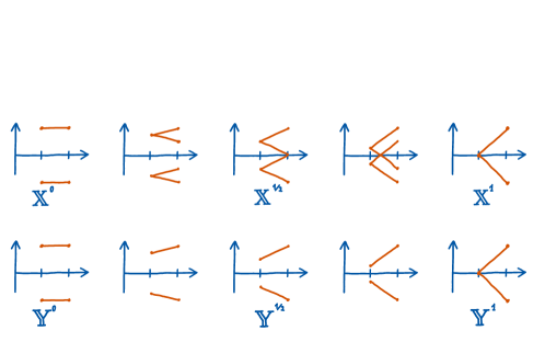
Figure 3. Comparison of the adapted Wasserstein interpolation $({\mathbb{X}}^{u})_{u\in[0,1]}$ and a classical Wasserstein interpolation $({\mathbb{Y}}^{u})_{u\in[0,1]}$ where the geodesic between martingales does not consist of martingales.

For ease of exposition, we will only check that the set of martingales is geodesically convex when restricting to geodesics given by interpolation processes. Knowing that all geodesics can be characterized this way modulo an external randomization, this assumption can in fact be made without loss of generality. Alternatively, a proof via our description of geodesic processes as geodesics on $\mathcal{P}_{p}(\mathcal{Z}_{1})$ in Theorem 5.10 is possible too, but less informative, and therefore left to the ambitious reader.

Simplified proof.

By Proposition 5.7, it remains to show that ${\rm M}_{p}$ is geodesically convex. To that end, let ${\mathbb{X}},{\mathbb{Y}}\in{\rm M}_{p}$ and let $({\mathbb{Z}}^{u})_{u\in[0,1]}$ be a constant speed geodesic connecting them, which, as already explained, is assumed to be given as the interpolation processes w.r.t. some $\pi\in\mathrm{Cpl}_{\mathrm{bc}}({\mathbb{X}},{\mathbb{Y}})$.

We need to show that, for given fixed $u\in[0,1]$, the processes ${\mathbb{Z}}^{u}$ is a martingale, too. To that end, let $1\leq s\leq t\leq N$ and write

$${\mathbb{E}}\left[Z^{u}_{t}\middle|\mathcal{F}^{{\mathbb{Z}}}_{s}\right] ={\mathbb{E}}_{\pi}\left[(1-u)X_{t}+uY_{t}\middle|\mathcal{F}^{{\mathbb{X}},{\mathbb{Y}}}_{s,s}\right]=(1-u){\mathbb{E}}\left[X_{t}\middle|\mathcal{F}^{{\mathbb{X}}}_{s}\right]+u{\mathbb{E}}\left[Y_{t}\middle|\mathcal{F}^{{\mathbb{Y}}}_{s}\right]=Z_{s}^{u}$$

where we use bicausality of $\pi$ in the form of Lemma 2.2, and the martingale property of both ${\mathbb{X}}$ and ${\mathbb{Y}}$. Hence ${\mathbb{Z}}^{u}$ is a martingale which completes the proof. ∎

Remark 5.13.

We chose $\mathcal{X}_{t}=\mathbb{R}^{d}$ in this section to lighten notation. However, Theorem 5.10 remains valid if all of the $\mathcal{X}_{t}$’s are geodesic space, with the obvious modifications, such as replacing $(1-u)X_{t}+uY_{t}$ in Definition 5.9 by (appropriately measurable selections of) geodesics between $X_{t}$ and $Y_{t}$.

6. Continuity w.r.t. $\mathcal{AW}_{p}$ and applications

We have argued in the introduction that the weak adapted distribution governs ‘all’ probabilistic aspects of a stochastic process. In this section we highlight this claim, and further show that several (optimization) problems involving stochastic processes continuously depend on the adapted distribution. And moreover, that quantitative estimates w.r.t. $\mathcal{A}\mathcal{W}_{p}$ are possible. Throughout this section we assume that $\mathcal{X}_{t}={\mathbb{R}}^{d}$ for every $1\leq t\leq N$.

6.1. Optimal stopping

Fix a non-anticipative function $c\colon({\mathbb{R}}^{d})^{N}\times\{1,\dots,N\}\to\mathbb{R}$ and set

(6.1) $$v_{c}({\mathbb{X}}):=\inf_{\tau\in\mathrm{ST}({\mathbb{X}})}{\mathbb{E}}[c_{\tau}(X)]$$

for ${\mathbb{X}}\in\mathcal{FP}$, where $\mathrm{ST}({\mathbb{X}})$ denotes the set of all $(\mathcal{F}_{t}^{\mathbb{X}})_{t=1}^{N}$-stopping times taking values in $\{1,\dots,N\}$. In Example 4.5 we have already seen that $v_{c}$ is well-defined on $\mathrm{FP}_{p}$ in the sense that the value of $v_{c}$ does not depend on the choice of representative.

Proposition 6.1 (Optimal stopping).

Let ${\mathbb{X}},{\mathbb{Y}}\in\mathrm{FP}$ such that $c_{1:N}(X)$ and $c_{1:N}(Y)$ are integrable. Then we have

$$v_{c}({\mathbb{X}})-v_{c}({\mathbb{Y}}) \leq\inf_{\pi\in\mathrm{Cpl}_{\mathrm{c}}({\mathbb{X}},{\mathbb{Y}})}{\mathbb{E}}_{\pi}\Big{[}\max_{1\leq t\leq N}|c_{t}(X)-c_{t}(Y)|\Big{]}.$$

In particular, the following hold.

1. If $c_{t}$ is continuous bounded for every $t$, then ${\mathbb{X}}\mapsto v_{c}({\mathbb{X}})$ is continuous on $\mathrm{FP}$ w.r.t. the weak adapted topology.

2. If $c_{t}$ is continuous and satisfies that $|c_{t}(\cdot)|\leq\alpha(1+|\cdot|^{p})$ for every $t$ and some $\alpha>0$, then ${\mathbb{X}}\mapsto v_{c}({\mathbb{X}})$ is continuous on $\mathrm{FP}_{p}$ w.r.t. $\mathcal{AW}_{p}$.

3. If $c_{t}$ is Lipschitz for every $t$, then ${\mathbb{X}}\mapsto v_{c}({\mathbb{X}})$ is $\mathcal{A}\mathcal{W}_{1}$-Lipschitz on $\mathrm{FP}_{1}$.

In Theorem 7.1 we will construct an example showing that the whole adapted distribution is required to control optimal stopping problems. Note that the non-quantitative version of Proposition 6.1 (i.e. continuity of optimal stopping for continuous $c$ that satisfies an adequate growth condition) already follows from Example 4.5.

Proof of Proposition 6.1.

The ‘in particular’ statement follows by symmetry from the first statement, so we shall only prove the first one. Its proof is similar to [12] and is included here for the convenience of the reader. Let $\varepsilon>0$ and $\tau^{\ast}\in\mathrm{ST}({\mathbb{Y}})$ be a stopping time such that ${\mathbb{E}}[c_{\tau^{\ast}}(Y)]\leq v_{c}({\mathbb{Y}})+\varepsilon$. Further let $\pi\in\mathrm{Cpl}_{\mathrm{c}}({\mathbb{X}},{\mathbb{Y}})$ and, for every $u\in[0,1]$, define

$$\sigma_{u}:=\min\left\{t\in\{1,\dots,N\}:\pi\left(\tau^{\ast}\leq t\middle|\mathcal{F}^{{\mathbb{X}},{\mathbb{Y}}}_{N,0}\right)\geq u\right\}.$$

By causality, c.f. Lemma 2.2, we have $\sigma_{u}\in\mathrm{ST}({\mathbb{X}})$, hence

$$v_{c}({\mathbb{X}}) \leq\inf_{u\in[0,1]}{\mathbb{E}}_{\pi}\left[c_{\sigma_{u}}(X)\right]\leq\int_{[0,1]}{\mathbb{E}}_{\pi}[c_{\sigma_{u}}(X)]\,du$$

$$=\sum_{t=0}^{N}\int_{[0,1]}{\mathbb{E}}_{\pi}\left[c_{t}(X)1_{\pi\left(\tau^{\ast}\leq t\middle|\mathcal{F}^{{\mathbb{X}},{\mathbb{Y}}}_{N,0}\right)\geq u>\pi\left(\tau^{\ast}\leq t-1|\mathcal{F}^{{\mathbb{X}},{\mathbb{Y}}}_{N,0}\right)}\right]\,du={\mathbb{E}}_{\pi}[c_{\tau^{\ast}}(X)].$$

In conclusion we obtain

$$v_{c}({\mathbb{X}})-v_{c}({\mathbb{Y}})\leq{\mathbb{E}}_{\pi}\left[c_{\tau^{\ast}}(X)-c_{\tau^{\ast}}(Y)\right]+\varepsilon\leq{\mathbb{E}}_{\pi}\left[\max_{1\leq t\leq N}|c_{t}(X)-c_{t}(Y)|\right]+\varepsilon,$$

which, as $\varepsilon>0$ and $\pi\in\mathrm{Cpl}_{\mathrm{c}}({\mathbb{X}},{\mathbb{Y}})$ were arbitrary, yields the assertion. ∎

6.2. American options and robust pricing

Working in the setup of e.g. [29], $X_{t}\in{\mathbb{R}}_{+}$ stands for the (discounted) price of a financial asset at a time $t\in\{1,\ldots,N\}$ and $x_{1}=X_{1}\in{\mathbb{R}}_{+}$ denotes the current price. One assumes that there exists a family of European derivatives, described by a (continuous and linearly bounded) family of functions $\phi_{i}:({\mathbb{R}}_{+})^{N}\to{\mathbb{R}},i\in I$ which are liquidly traded in the market, meaning that the respective prices $p_{i},i\in I$ are specified from externally given data. The set of all calibrated models  consists of all martingales with mean $x_{1}$ which correctly reproduce the prices given by the market, i.e. in mathematical terms

(6.2) $$\mathrm{M}_{I}:=\{{\mathbb{X}}\in\mathrm{M}_{1}:X_{1}=x_{1},{\mathbb{E}}[\phi_{i}(X)]=p_{i},i\in I\}.$$

A common assumption is

(CC) $$\{\phi_{i}\colon i\in I\} X_{N} {\rm M}_{I}\neq\emptyset$$ contains all call options written on and .

Going back to a famous observation of Breeden-Litzenberger [37], this implies the following basic fundamental fact:

Proposition 6.2.

Under assumption (CC) the set $\{\mathscr{L}({\mathbb{X}}):{\mathbb{X}}\in\mathrm{M}_{I}\}$ is $\mathcal{W}_{1}$-compact.

A direct consequence is that for a further (continuous, linearly bounded) European derivative $\Phi:({\mathbb{R}}_{+})^{N}\to{\mathbb{R}},i\in I$ the set of possible arbitrage free prices consists of the interval $\big{[}\inf_{{\mathbb{X}}\in\mathrm{M}_{I}}{\mathbb{E}}[\Phi(X)],$ $\sup_{{\mathbb{X}}\in\mathrm{M}_{I}}{\mathbb{E}}[\Phi(X)]\big{]}$, where the endpoints are attained for ‘extremal models’. Proposition 6.2 as well as various extensions of it play a crucial role for the duality theory as well as the characterization of extremal models in robust finance, see [33, 27, 54, 40] among many others.

A particular limitation of Proposition 6.2 is that it allows only to consider derivatives with a European payoff structure, but neglects derivatives with an American exercise structure, where the buyer may choose when to exercise and the buyers price in a model ${\mathbb{X}}$ equals

(6.3) $$\sup\{{\mathbb{E}}[\Phi(X)]:\tau\in{\rm ST}({\mathbb{X}})\}.$$

Apart from a few important exceptions (see [26, 59, 8]) the robust finance literature is focused on the case of European derivatives. The simple reason is that going beyond the standard European case requires an adequate topology on processes with a non trivial filtration, which was hitherto unavailable. As derivatives with American exercise structure are more common than European derivatives it is highly desirable to extend the existing theory to this case. As a consequence of our results we obtain.

Proposition 6.3.

Assume that $\{\phi_{i}:i\in I\}$ is a family of derivatives with linearly bounded continuous payoffs and European or American exercise structures. Under assumption (CC), the set $\{{\mathbb{X}}:{\mathbb{X}}\in\mathrm{M}_{I}\}$ is $\mathcal{A}\mathcal{W}_{1}$-compact. Moreover, for a European or American derivative with continuous linearly bounded payoff $\Phi:({\mathbb{R}}_{+})^{N}\to{\mathbb{R}}$, the lower/upper pricing bounds for the derivative $\Phi$ are attained.

Proof.

This is a direct consequence of Prokhorov’s theorem in our setting (Theorem 5.1), Proposition 6.3, and the continuity of optimal stopping (Proposition 6.1). ∎

6.3. Utility maximization

Let $U\colon{\mathbb{R}}\to{\mathbb{R}}$ be an increasing concave (utility) function, and denote by $U^{\prime}$ the left-continuous version of the derivative. Denote by $\mathcal{H}({\mathbb{X}})$ the set of all $(\mathcal{F}^{{\mathbb{X}}}_{t})_{t=1}^{N}$-predictable processes $H$ that are bounded by 1, and by $(H\cdot X)_{t}:=\sum_{s=1}^{t-1}H_{s+1}(X_{s+1}-X_{s})$ the discrete-time stochastic integral of $H$ w.r.t. $X$. For $C\colon({\mathbb{R}}^{d})^{N}\to{\mathbb{R}}$ and ${\mathbb{X}}\in\mathrm{FP}_{p}$, denote by $u({\mathbb{X}})$ the value of the utility maximization problem with random endowment $C$, that is,

$$u({\mathbb{X}}):=\sup_{H\in\mathcal{H}({\mathbb{X}})}{\mathbb{E}}[U(C(X)+(H\cdot X)_{N})].$$

In [11, Theorem 1.8] it is shown that $u({\mathbb{X}})$ depends continuously on ${\mathbb{X}}$ (w.r.t. $\mathcal{AW}_{p}$) when restricting to plain processes (i.e. to ${\mathbb{X}}$ whose filtration is generated only by their paths). In the context of utility maximization, however, it is of central importance to also understand the effect that changes of the information/filtration of ${\mathbb{X}}$ have to $u({\mathbb{X}})$, and the following result extends [11, Theorem 1.8] to the general setting.

Theorem 6.4.

Let $C\colon{\mathbb{R}}^{N}\to{\mathbb{R}}$ be Lipschitz continuous and assume that there exists $\alpha$ such that $U^{\prime}(\cdot)\leq\alpha(1+|\cdot|^{p-1})$. Then, for every $R>0$ there is a constant $K$ (depending only on $R$, $\alpha$ and the Lipschitz constant of $C$) such that

$$\left|u({\mathbb{X}})-u({\mathbb{Y}})\right|\leq K\cdot\mathcal{AW}_{p}({\mathbb{X}},{\mathbb{Y}})$$

for every ${\mathbb{X}},{\mathbb{Y}}\in\mathrm{FP}_{p}$ with $\mathcal{AW}_{p}({\mathbb{X}},0),\mathcal{AW}_{p}({\mathbb{Y}},0)\leq R$.

Proof.

For simplicity, we assume that $C=0$ and focus on $p=1$ (i.e. $U$ is Lipschitz); the modifications needed for the general case are minimal and follow e.g. as detailed in [11]. Let $H^{\ast}\in\mathcal{H}({\mathbb{X}})$ be (almost) optimal for $u({\mathbb{X}})$ and let $\pi\in\mathrm{Cpl}_{\mathrm{bc}}({\mathbb{X}},{\mathbb{Y}})$ be (almost) optimal for $\mathcal{AW}_{1}({\mathbb{X}},{\mathbb{Y}})$. Define $G_{t}:={\mathbb{E}}_{\pi}[H_{t}^{\ast}|\mathcal{F}^{{\mathbb{X}},{\mathbb{Y}}}_{0,N}]$ for every $t$. Clearly $G$ is bounded by 1, and by bicausality of $\pi$, $G_{t}$ is $\mathcal{F}^{{\mathbb{Y}}}_{t}$-measurable (see Lemma 2.2); hence $G\in\mathcal{H}({\mathbb{Y}})$. It follows that

$$u({\mathbb{Y}})\geq{\mathbb{E}}[U((G\cdot Y)_{N})]={\mathbb{E}}_{\pi}[U({\mathbb{E}}_{\pi}[(H^{\ast}\cdot Y)_{N}\mid|\mathcal{F}^{{\mathbb{X}},{\mathbb{Y}}}_{0,N}])].$$

By concavity of $U$ and Jensen’s inequality, followed by Lipschitz continuity of $U$,

$$u({\mathbb{Y}})\geq{\mathbb{E}}_{\pi}\left[U\left((H^{\ast}\cdot Y)_{N}\right)\right] ={\mathbb{E}}_{\pi}\left[U\left((H^{\ast}\cdot X)_{N}+(H^{\ast}\cdot(Y-X))_{N}\right)\right]$$

$$\geq{\mathbb{E}}_{\pi}\left[U\left((H^{\ast}\cdot X)_{N}\right)\right]-L{\mathbb{E}}_{\pi}\left[|(H^{\ast}\cdot(Y-X))_{N}|\right]$$

where $L$ is the Lipschitz constant of $U$. It remains to note that $|(H^{\ast}\cdot(Y-X))_{N}|\leq 2\sum_{t=1}^{N}|X_{t}-Y_{t}|$, hence $u({\mathbb{Y}})\geq u({\mathbb{X}})-2L\mathcal{AW}_{1}({\mathbb{X}},{\mathbb{Y}})$. Reversing the roles of ${\mathbb{X}}$ and ${\mathbb{Y}}$ proves the claim. ∎

Remark 6.5.

As explained in [11, Section 3.3], in the context of optimization problems involving stochastic integrals and (semi-)martingales, it is more natural to define $\mathcal{A}\mathcal{W}_{p}$ with a different cost function instead of ${\mathbb{E}}[d^{p}(X,Y)]$, namely with ${\mathbb{E}}[|\langle M^{{\mathbb{X}}}-M^{{\mathbb{Y}}}\rangle|^{p/2}+|A^{{\mathbb{X}}}-A^{{\mathbb{Y}}}|_{\rm var}^{p}]$ where ${\mathbb{X}}=M^{{\mathbb{X}}}+A^{{\mathbb{X}}}$ denotes the Doob-decomposition, $\langle\cdot\rangle$ the quadratic variation, and $|\cdot|_{\rm var}$ the first variation norm. Clearly, this modification of $\mathcal{A}\mathcal{W}_{p}$ is also possible (and reasonable) in the present setting.

6.4. Stochastic control

Optimal stopping and utility maximization are basic stochastic control problems involving processes and we have shown in Proposition 6.1 and Theorem 6.4 that their values are continuous w.r.t. the adapted Wasserstein distance. As it happens, this is the general principle for stochastic control problems.

For example, if $J\colon({\mathbb{R}}^{d})^{N}\times\mathbb{R}^{N-1}\times(\mathbb{R}^{d})^{N}\to\mathbb{R}$ is convex in the second and third argument, a similar reasoning as used for the proof of Theorem 6.4 shows that under suitable continuity and growth assumptions on $J$,

$${\mathbb{X}}\mapsto\inf_{H\in\mathcal{H}({\mathbb{X}})}{\mathbb{E}}\Big{[}J\Big{(}X,((H\cdot X)_{t})_{t=2}^{N},H\Big{)}\Big{]},$$

is (locally Lipschitz) continuous w.r.t. $\mathcal{A}\mathcal{W}_{p}$.

We refer to [11] for a more elaborate analysis of such problems in a mathematical finance context. In particular, using the results of the present paper, the results of [11] for the stability of superhedging, risk based headging and utility indifference pricing (which are formulated only for processes endowed with their raw filtration) extend to processes with arbitrary filtrations.

6.5. Conditional McKean-Vlasov control

Denote by $\mathcal{A}({\mathbb{X}})$ the set of all $(\mathcal{F}^{{\mathbb{X}}}_{t})_{t=1}^{N}$-adapted processes that are bounded by 1 and let ${\mathbb{B}}$ be a discrete-time Brownian motion. For $\alpha\in\mathcal{A}({\mathbb{B}})$ consider the controlled process ${\mathbb{X}}^{{\mathbb{B}},\alpha}$, defined recursively via $X^{{\mathbb{B}},\alpha}_{1}=0$ and

$$X^{{\mathbb{B}},\alpha}_{t+1}:=G_{t+1}\left(X^{{\mathbb{B}},\alpha}_{t},\alpha_{t},\mathcal{L}(X_{t}^{{\mathbb{B}},\alpha}),B_{t+1}-B_{t}\right),$$

where $G_{t+1}\colon{\mathbb{R}}^{d}\times{\mathbb{R}}^{d}\times\mathcal{P}_{p}({\mathbb{R}}^{d})\times{\mathbb{R}}^{d}\to[0,1]$ is some fixed continuous function prescribing the dynamics of $X^{{\mathbb{B}},\alpha}$. Further let $J\colon({\mathbb{R}}^{d})^{T}\times({\mathbb{R}}^{d})^{T}\times\mathcal{P}_{p}(({\mathbb{R}}^{d})^{T})\to[0,1]$ be continuous and consider the McKean-Vlasov control problem in its weak formulation:

(6.4) $$\inf_{{\mathbb{B}}\text{ is Bronwian motion and }\alpha\in\mathcal{A}({\mathbb{B}})}{\mathbb{E}}\left[J\left(X^{{\mathbb{B}},\alpha},\alpha,\mathcal{L}(X^{{\mathbb{B}},\alpha}|\mathcal{F}^{{\mathbb{B}}}_{t})_{t=1}^{N}\right)\right];$$

we refer to [84] for more background on problems of the type (6.4). Based on Prokhorov’s theorem for filtered processes, it is straightforward to show that a solution to (6.4) exists:

Proposition 6.6.

The infimum over all Brownian motions ${\mathbb{B}}$ and controls $\alpha\in\mathcal{A}({\mathbb{B}})$ in (6.4) is attained.

Sketch of proof.

Let $({\mathbb{B}}^{k},\alpha^{k})_{k}$ be a minimizing sequence for (6.4) (in particular, $\alpha^{k}\in\mathcal{A}({\mathbb{B}}^{k})$), and set ${\mathbb{Y}}^{k}:=(\Omega^{{\mathbb{B}}^{k}},\mathcal{F}^{{\mathbb{B}}^{k}},{\mathbb{P}}^{{\mathbb{B}}^{k}},(\mathcal{F}_{t}^{{\mathbb{B}}^{k}})_{t=1}^{N},(B^{k},\alpha^{k}))$. By Theorem 5.1, the set $\{{\mathbb{Y}}^{k}:k\in\mathbb{N}\}$ is relatively compact, hence there exists

$${\mathbb{Y}}=\left(\Omega,\mathcal{F},{\mathbb{P}},(\mathcal{F}_{t})_{t=1}^{N},(B,\alpha)\right)\in\mathrm{FP}_{p}$$

such that (potentially after passing to a subsequence) $\mathcal{AW}_{p}({\mathbb{Y}}^{k},{\mathbb{Y}})\to 0$. It is straightforward to verify that ${\mathbb{B}}=(\Omega,\mathcal{F},{\mathbb{P}},(\mathcal{F}_{t})_{t=1}^{N},B)$ is a Brownian motion and that $\alpha\in\mathcal{A}({\mathbb{B}})$. Further, since each $G_{t}$ is continuous,

$$(X^{{\mathbb{B}}^{k},\alpha^{k}},{\alpha^{k}},(\mathscr{L}(X^{{\mathbb{B}}^{k},\alpha^{k}}|\mathcal{F}_{t}^{{\mathbb{B}}^{k}}))_{t=1}^{N})\to(X^{{\mathbb{B}},\alpha},\alpha,(\mathscr{L}(X^{{\mathbb{B}},\alpha}|\mathcal{F}_{t}))_{t=1}^{N})\quad\text{in distribution},$$

as $k\to\infty$. The claim now readily follows form continuity of $J$. ∎

6.6. Weak optimal transport

Motivated by applications to functional inequalities, Gozlan et. al. [53] introduced the weak optimal transport problem, which extends classical transport to ‘non-linear’ costs $c\colon{\mathbb{R}}^{d}\times\mathcal{P}({\mathbb{R}}^{d})\to[0,\infty)$. Given marginal distributions $\mu_{1},\mu_{2}$ on ${\mathbb{R}}^{d}$, the task is

(WOT) $$\text{minimize}\quad{\mathbb{E}}[c(X_{1},\mathcal{L}(X_{2}|X_{1}))]\quad\text{over couplings $(X_{1},X_{2})$ s.t.\ $\mathscr{L}(X_{1})=\mu_{1}$, $\mathscr{L}(X_{2})=\mu_{2}$}.$$

Weak transport preserves enough structure from the classical case to allow for a useful theory while being sufficiently general to capture many problems that lie outside the scope of transport theory, see [20] for an overview. Cornerstone results in weak optimal transport (existence of optimizers, duality, geometric characterization of optimal couplings, stability in the data) were shown in the generality of classical transport only in [17, 3, 31], relying on two-period results of the current article and the two period version of Theorem 1.7. In analogy to classical transport, the key idea is to relax (WOT) and consider

(6.5) $$\inf\big{\{}{\mathbb{E}}[c(X_{1},\mathcal{L}(X_{2}|\mathcal{F}_{1}))]:\text{${\mathbb{X}}\in\mathcal{FP}$ satisfies $\mathscr{L}(X_{1})=\mu_{1}$, $\mathscr{L}(X_{2})=\mu_{2}$}\big{\}}.$$

By Theorem 1.7 this is an optimization over a compact set which of course admits minimizers under the usual assumption of lower semi-continuity. Indeed (6.5) can be viewed as a classical linear optimization problem over probabilities on $\mathcal{Z}_{1}$.

In several weak transport problems it is natural to consider not just two marginal constraints, but arbitrarily many (relaxed martingale transport [54], robust pricing of VIX-futures [55], model-independence in fixed income markets following [3], multi-marginal Skorokhod embedding [41, 28]). In view of this, we propose the $N$-marginal weak transport problem

(6.6) $$\inf\big{\{}{\mathbb{E}}[c(\mathrm{ip}({\mathbb{X}}))]:\text{ ${\mathbb{X}}\in\mathcal{FP}$ satisfies $\mathscr{L}(X_{1})=\mu_{1}$,\ldots,$\mathscr{L}(X_{N})=\mu_{N}$}\big{\}}.$$

As above this is an optimization problem over a compact set, which corresponds to a linear optimization problem of probabilities on $\mathcal{Z}_{1}$, susceptible to classical convex analysis.

6.7. $\mathcal{A}\mathcal{W}_{p}$-barycenters

The $\mathcal{A}\mathcal{W}_{p}$-barycenter of two stochastic processes ${\mathbb{Z}}^{0},{\mathbb{Z}}^{1}\in\mathrm{FP}_{p}$ is the minimizer of

$$\inf_{{\mathbb{X}}\in\mathrm{FP}_{p}}\frac{1}{2}\left(\mathcal{A}\mathcal{W}_{p}^{p}({\mathbb{Z}}^{0},{\mathbb{X}})+\mathcal{A}\mathcal{W}_{p}^{p}({\mathbb{Z}}^{1},{\mathbb{X}})\right).$$

Clearly, this minimization problem is attained by the connecting constant speed geodesic at time $1/2$ (which exist thanks to Theorem 5.10). More generally, one can ask whether a distribution on the stochastic processes $\gamma\in\mathcal{P}_{p}(\mathrm{FP}_{p})$ has an $\mathcal{A}\mathcal{W}_{p}$-barycenter ${\mathbb{X}}^{\ast}\in\mathrm{FP}_{p}$, that is, a minimizer of

(6.7) $$\inf_{{\mathbb{X}}\in\mathrm{FP}_{p}}\int\mathcal{A}\mathcal{W}_{p}^{p}({\mathbb{Z}},{\mathbb{X}})\,\gamma(d{\mathbb{Z}}).$$

Theorem 6.7.

Let $\gamma\in\mathcal{P}_{p}(\mathrm{FP}_{p})$. Then there exists ${\mathbb{X}}^{\ast}\in\mathrm{FP}_{p}$ minimizing (6.7).

Proof.

Corollary 3.12 implies that $({\mathbb{X}},{\mathbb{Z}})\mapsto\mathcal{A}\mathcal{W}_{p}({\mathbb{X}},{\mathbb{Z}})$ is lower semicontinuity w.r.t. the weak adapted topology. Hence, it follows that

$$F({\mathbb{X}}):=\int\mathcal{A}\mathcal{W}_{p}^{p}({\mathbb{Z}},{\mathbb{X}})\,\gamma(d{\mathbb{Z}}),$$

is lower semicontinuity on $\mathrm{FP}_{p}$ w.r.t. the weak adapted topology. Since $F({\mathbb{X}})<\infty$ for ${\mathbb{X}}\in\mathrm{FP}$ if and only if ${\mathbb{X}}\in\mathrm{FP}_{p}$, it suffices to show relative compactness of the sublevel set

(6.8) $$\Big{\{}{\mathbb{X}}\in\mathrm{FP}\colon F({\mathbb{X}})\leq\inf_{{\mathbb{Y}}\in\mathrm{FP}}F({\mathbb{Y}})+\varepsilon\Big{\}},$$

where $\varepsilon>0$, in the weak adapted topology. Note that the moments of ${\mathbb{X}}\in\mathrm{FP}_{p}$ can be controlled as follows:

(6.9) $$\sum_{t=1}^{N}{\mathbb{E}}\left[|X_{t}|^{p}\right]=\mathcal{A}\mathcal{W}_{p}^{p}({\mathbb{X}},0)\leq 2^{p-1}\!\int\!\mathcal{A}\mathcal{W}_{p}^{p}({\mathbb{Z}},{\mathbb{X}})\!+\!\mathcal{A}\mathcal{W}_{p}^{p}(0,{\mathbb{Z}})\,\gamma(dz)=2^{p-1}\left(F({\mathbb{X}})\!+\!F(0)\right).$$

By Theorem 5.1, relative compactness of the set (6.8) is equivalent to tightness of the laws. Tightness of (6.8) follows from standard arguments since the $p$-moments are uniformly bounded by (6.9) and $\{x\in{\mathbb{R}}^{d}\colon|x|\leq K\}$ is compact for $K>0$. ∎

6.8. The Doob-decomposition

Our final example deals with continuity of the Doob-decomposition. Recall that the Doob-decomposition ${{\mathbb{D}}}^{{\mathbb{X}}}$ of a filtered process ${\mathbb{X}}$ is given by

$${{\mathbb{D}}}^{{\mathbb{X}}}:=(\Omega^{{\mathbb{X}}},\mathcal{F}^{{\mathbb{X}}},(\mathcal{F}^{{\mathbb{X}}}_{t})_{t=1}^{N},P^{{\mathbb{X}}},(M_{t},A_{t})_{t=1}^{N}),$$

where $M+A=X$ is the unique decomposition of $X$ such that $A_{1}=0$, $M=M^{{\mathbb{X}}}$ is a martingale and $A=A^{{\mathbb{X}}}$ is $(\mathcal{F}^{{\mathbb{X}}}_{t})_{t=1}^{N}$-predictable. (Of course, $X$ is a sub-martingale if and only if the process $A$ is increasing.)

Proposition 6.8.

The following chain of inequalities holds

(6.10) $$2^{\frac{1-p}{p}}\mathcal{A}\mathcal{W}_{p}({\mathbb{X}},{\mathbb{Y}})\leq\mathcal{A}\mathcal{W}_{p}({{\mathbb{D}}}^{{\mathbb{X}}},{{\mathbb{D}}}^{{\mathbb{Y}}})\leq c\cdot\mathcal{A}\mathcal{W}_{p}({\mathbb{X}},{\mathbb{Y}})$$

for all ${\mathbb{X}},{\mathbb{Y}}\in\mathrm{FP}_{p}$, where $c=c(p,N)$ is a constant depending only on $p$ and $N$.

Recall that the predictable process $A^{\mathbb{X}}$ of the Doob-decomposition of ${\mathbb{X}}\in\mathrm{FP}_{p}$ is given by

$$A^{{\mathbb{X}}}_{t}:=\sum_{s=1}^{t-1}{\mathbb{E}}[X_{s}-X_{s-1}|\mathcal{F}^{{\mathbb{X}}}_{s}]$$

for $2\leq t\leq N$ and $M^{{\mathbb{X}}}:=X-A^{{\mathbb{X}}}$. Thus, $A_{t}$ can be viewed as an adapted function of rank 1, that is $A_{t}\in{\mathrm{AF}}[1]$ and similarly $M_{t}\in{\mathrm{AF}}[1]$. Building upon this observation, it is not hard to deduce $\mathcal{A}\mathcal{W}_{p}$-continuity of ${\mathbb{X}}\mapsto{\mathbb{D}}^{{\mathbb{X}}}$.

Proof of Proposition 6.8.

Fix ${\mathbb{X}},{\mathbb{Y}}\in\mathrm{FP}_{p}$ and note that, as the filtration of a filtered process and its Doob-decomposition coincide by definition, we have that

$$\mathrm{Cpl}_{\mathrm{bc}}({\mathbb{X}},{\mathbb{Y}})=\mathrm{Cpl}_{\mathrm{bc}}({\mathbb{D}}^{{\mathbb{X}}},{\mathbb{D}}^{{\mathbb{Y}}}).$$

The first inequality in (6.10) is immediate from Jensen’s inequality. The triangle inequality together with Jensen’s inequality show

(6.11) $$|(M^{{\mathbb{X}}}-M^{\mathbb{Y}},A^{{\mathbb{X}}}-A^{\mathbb{Y}})|_{p}^{p}\leq 2^{p-1}|X-Y|^{p}+(2^{p-1}+1)|A^{\mathbb{X}}-A^{\mathbb{Y}}|^{p}.$$

By definition of $A^{\mathbb{X}}$ and $A^{\mathbb{Y}}$ we have for $2\leq t\leq N$

$$A^{{\mathbb{X}}}_{t}-A^{{\mathbb{Y}}}_{t}=\sum_{s=2}^{t}{\mathbb{E}}_{\pi}\left[X_{s}-X_{s-1}-(Y_{s}-Y_{s-1})\middle|\mathcal{F}^{{\mathbb{X}},{\mathbb{Y}}}_{s,s}\right].$$

Again, Jensen’s inequality implies

$${\mathbb{E}}_{\pi}[|A^{{\mathbb{X}}}-A^{{\mathbb{Y}}}|^{p}]^{\frac{1}{p}} \leq\Big{(}\sum_{t=2}^{N}t^{p-1}\sum_{s=2}^{t}{\mathbb{E}}_{\pi}[|X_{s}-X_{s-1}-(Y_{s}-Y_{s-1})|^{p}]\Big{)}^{\frac{1}{p}}$$

(6.12) $$\leq\big{(}N2^{p}N^{p-1}{\mathbb{E}}_{\pi}[|X-Y|^{p}]\big{)}^{\frac{1}{p}}$$

for every $\pi\in\mathrm{Cpl}_{\mathrm{bc}}({\mathbb{X}},{\mathbb{Y}})$. In conclusion, suitably combining (6.11) and (6.12) leads to the second inequality in (6.10). ∎

6.9. Numerical and statistical aspects

In view of applications, the numerical computation of the adapted Wasserstein distance is of crucial importance and has been recently studied in [87, 44, 25]. In fact, these papers consider more general adapted transport problems between stochastic processes ${\mathbb{X}}$ and ${\mathbb{Y}}$ of the form

(6.13) $$\inf_{\pi\in\mathrm{Cpl}_{\mathrm{bc}}({\mathbb{X}},{\mathbb{Y}})}\mathbb{E}_{\pi}\left[c(X,Y)\right],$$

where $c$ is a continuous function. In order to briefly explain the methodology, suppose that the processes ${\mathbb{X}}$ and ${\mathbb{Y}}$ are both discrete, i.e. plain and only take finitely many values. (We remark that for general processes ${\mathbb{X}}$ and ${\mathbb{Y}}$ that are not necessarily discrete, one may replace them first by discrete approximations e.g. as in Proposition 5.5). In this case, solving (6.13) is equivalent to solving a linear program (see e.g.  [80, Section 8] and [44, Section 3.4] for more details). The recursive structure of bicausal couplings allows to solve the linear program via a dynamic programming principle (DPP) involving one-step classical optimal transport problems (see [81, Chapter 2.10.3]). In the current setting, the value functions $V_{t}\colon\mathcal{Z}_{1:t}\times\mathcal{Z}_{1:t}\to{\mathbb{R}}$ are recursively given by

$$V_{N}(\hat{z}_{1:N},\check{z}_{1:N}):=c(\hat{z}_{1:N}^{-},\check{z}_{1:N}^{-}),\quad V_{t}(\hat{z}_{1:t},\check{z}_{1:t}):=\inf_{\pi\in\mathrm{Cpl}(\hat{z}^{+}_{t},\check{z}_{t}^{+})}{\mathbb{E}}_{\pi}[V_{t+1}[\hat{z}_{1:t},\cdot,\check{z}_{1:t}^{-},\cdot]],$$

for $t=N-1,\ldots,0$ with the convention that $\hat{z}_{0}^{+}:=\mathscr{L}(\mathrm{ip}_{1}({\mathbb{X}}))$ and $\check{z}_{0}^{+}:=\mathscr{L}(\mathrm{ip}_{1}({\mathbb{Y}}))$. Then $V_{0}$ is precisely the optimal value (6.13) and the values of $V_{t}$ can be computed efficiently e.g. via Sinkhorn’s algorithm (see [87]). Based on the DPP formulation, a fitted value iteration method is proposed in [25]. There the value function of the DPP is iteratively empirically estimated and then approximated by neural networks that minimize an empirical loss. Another recent approach builds on establishing a bicausal version of the Sinkhorn algorithm (see [44]). For comprehensive comparisons of these methods, we refer to [44] and [25]. Furthermore, in [98], a minimax reformulation is proposed where the infimum is taken over all couplings and the supremum over an adequate class of functions penalizing the causality constraint. Both families of functions are then parametrized by neural networks and trained by an adversarial algorithm. In a continuous time framework, [35] establishes a Hamilton-Jacobi-Bellman equation for the value function.

The estimation of processes w.r.t. $\mathcal{AW}_{p}$ from statistical data was studied in [13] under the assumption of bounded values and later extended in [4] (see also [83, 52]). Roughly put, while the classical empirical measure does not converge to its population counterpart in the weak adapted topology (nor do e.g. the values of the corresponding optimal stopping problems) one can construct a modified empirical measure (based on clustering ideas) which does converge in the weak adapted topology. In fact, the rate of convergence of that estimator (w.r.t. $\mathcal{A}\mathcal{W}_{p}$) is similar to the (optimal) rate of convergence of the classical empirical measure (w.r.t. $\mathcal{W}_{p}$).

7. An important example

Fix $N\geq 2$ and recall that, by Theorem 4.11, the relation $\sim_{N-1}$ is equal to the relation $\sim_{\infty}$, which again coincides with the relation induced by $\mathcal{A}\mathcal{W}_{p}$.

A natural question left open in Section 4 and Section 5 is what rank of the adapted distribution is necessary to govern probabilistic properties of stochastic processes. For instance, we have seen in Example 4.5 that the adapted distribution of rank 1 suffices for preserving the notion of being a martingale. However, we will see that rank 1 equivalence is not sufficient in general. Rather Theorem 4.11 is sharp: $\sim_{N-2}$ does not imply $\sim_{N-1}$. In fact, we show that there exist filtered processes that are $\sim_{N-2}$ equivalent but lead to different values for an optimal stopping problem.

Theorem 7.1.

Let $N\geq 2$. There exist ${\mathbb{X}},{\mathbb{Y}}\in\mathrm{FP}_{p}$ with ${\mathbb{X}}\sim_{N-2}{\mathbb{Y}}$ and a bounded, continuous non-anticipative function $c\colon\mathcal{X}\times\{1,\dots,N\}\to\mathbb{R}$ such that $v_{c}({\mathbb{X}})\neq v_{c}({\mathbb{Y}})$ (compare (6.1) for the definition of $v_{c}$).

In particular, using Proposition 6.1 and Theorem 4.11, this implies that ${\mathbb{X}}\sim_{N-1}{\mathbb{Y}}$. More generally, we will show in the following that as long as $k\leq N-1$, the relation $\sim_{k}$ strictly refines the relation $\sim_{k-1}$.

Proposition 7.2.

Let $N\geq 2$ and let $1\leq k\leq N-1$. Then there are ${\mathbb{X}},{\mathbb{Y}}\in\mathrm{FP}_{p}$ with representatives defined on the same filtered probability space such that

1. $f({\mathbb{X}})=f({\mathbb{Y}})$ for every $f\in\mathrm{AF}[k-1]$,

2. ${\mathbb{E}}[f({\mathbb{X}})]\neq{\mathbb{E}}[f({\mathbb{Y}})]$ for some $f\in\mathrm{AF}[k]$.

The processes ${\mathbb{X}}$ and ${\mathbb{Y}}$ will be constructed on a common probability space consisting of $2^{N-1}$ atoms, satisfy $X=Y$ and $X_{t}=Y_{t}=0$ for $t\leq N-1$, and only their respective filtrations will differ.

7.1. Proof of Proposition 7.2

This section is devoted to the proof of Proposition 7.2 which will then be used to establish Theorem 7.1. In fact, we shall first concentrate on Proposition 7.2 with $k=N-1$, and later conclude for general $k$ via a simple argument.

The construction of ${\mathbb{X}}$ and ${\mathbb{Y}}$ is recursive, and we shall start with $N=2$. Consider the probability space consisting of two elements, say $\{0,1\}$, with the uniform measure, and let $U$ be the identity map, that is, ${\mathbb{P}}(U=1)={\mathbb{P}}(U=0)=1/2$. Now define the filtered processes ${\mathbb{X}}$ and ${\mathbb{Y}}$ via

$$X:=Y:=(0,U),\quad\mathcal{F}_{1}^{\mathbb{X}}:=\{\emptyset,\Omega\}\text{ and }\mathcal{F}_{1}^{\mathbb{Y}}:=\mathcal{F}_{2}^{\mathbb{Y}}:=\mathcal{F}_{2}^{\mathbb{X}}:=\sigma(U)$$

Then the following holds.

Lemma 7.3.

${\mathbb{X}}$ and ${\mathbb{Y}}$ satisfy the claim in Proposition 7.2 for $N=2$.

Proof.

Adapted functions of rank $0$ depend only on the process itself and not on the filtration, hence $f({\mathbb{X}})=f({\mathbb{Y}})$ for all $f\in\mathrm{AF}[0]$. That is, part (i) of Proposition 7.2 is true. On the other hand, one computes

$${\mathbb{E}}\left[g(X_{2})|\mathcal{F}_{1}^{\mathbb{X}}\right]={\mathbb{E}}[g(U)],\quad\quad{\mathbb{E}}\left[g(X_{2})|\mathcal{F}_{1}^{\mathbb{Y}}\right]=g(U)$$

for every bounded, measurable function $g\colon\mathbb{R}\to\mathbb{R}$. Now define $f\in\mathrm{AF}$ by

$$f:=\varphi((g|1)),\quad\text{ where }\varphi=t\mapsto t^{2}\wedge 1\text{ and }g:=x\mapsto(0\vee x)\wedge 1$$

so that $f$ has rank $1$. Then

$$f({\mathbb{X}})={\mathbb{E}}\left[X_{2}|\mathcal{F}_{1}^{\mathbb{X}}\right]^{2}=1/4,\quad\quad f({\mathbb{Y}})={\mathbb{E}}\left[X_{2}|\mathcal{F}_{1}^{\mathbb{Y}}\right]^{2}=X_{2}.$$

As ${\mathbb{E}}[f({\mathbb{Y}})]=1/2$, this proves the second part of Proposition 7.2. ∎

Now assume that, in a $(N-1)$-time step framework, we have constructed filtered processes ${\mathbb{X}}$ and ${\mathbb{Y}}$ which satisfy Proposition 7.2 (where $N\geq 3$). We shall construct new filtered processes ${\mathbb{X}}^{\mathrm{n}}$ and ${\mathbb{Y}}^{\mathrm{n}}$ in an $N$-time step framework for which the statement of the lemma remains true. At this particular instance the superscript ‘$\mathrm{n}$’ stands for ‘new’.

At this point, we enrich the filtered probability space of ${\mathbb{X}}$ and ${\mathbb{Y}}$ by an independent random variable $V$ (i.e. $V$ is independent of $\mathcal{F}_{N-1}^{\mathbb{X}}\vee\mathcal{F}_{N-1}^{\mathbb{Y}}$) in the following manner: When $(\Omega,\mathcal{F},{\mathbb{P}})$ denotes the probability space of ${\mathbb{X}}$ and ${\mathbb{Y}}$, we consider the new probability space

(7.1) $$\Big{(}\Omega^{\mathrm{n}}:=\{0,1\}\times\Omega\,,\,\mathcal{F}^{\mathrm{n}}:=\mathcal{B}(\{0,1\})\otimes\mathcal{F}\,,\,{\mathbb{P}}^{\mathrm{n}}:=\frac{1}{2}\left(\delta_{0}\otimes{\mathbb{P}}+\delta_{1}\otimes{\mathbb{P}}\right)\Big{)}.$$

We write $V\colon\Omega^{\mathrm{n}}\to\{0,1\}$ for the projection onto the first coordinate. In other words, we can think of $V$ as a coin-flip which is independent of everything that was constructed so far. Further we view $(\mathcal{G}_{t}^{\mathbb{X}})_{t=1}^{N}:=(\mathcal{F}_{t-1}^{\mathbb{X}})_{t=1}^{N-1}$ as a filtration on (7.1); similarly for $(\mathcal{G}^{{\mathbb{Y}}}_{t})_{t=1}^{N}$ (recall here that $\mathcal{F}_{0}^{\mathbb{X}}=\mathcal{F}_{0}^{\mathbb{Y}}$ are the trivial $\sigma$-algebras by convention). Then, by slight abuse of notation, we can view ${\mathbb{X}}$ and ${\mathbb{Y}}$ as processes defined on $\Omega^{\mathrm{n}}$, namely be identifying ${\mathbb{X}}$ with $(0,X)$ and filtration $(\mathcal{G}^{{\mathbb{X}}}_{t})_{t=1}^{N}$ and similarly for ${\mathbb{Y}}$. By independence of $V$, this clearly does not affect any properties of the processes. Define the processes ${\mathbb{X}}^{\mathrm{n}}$ and ${\mathbb{Y}}^{\mathrm{n}}$ on the probability space (7.1) via

$$X^{\mathrm{n}}:= Y^{\mathrm{n}}:=(0,X)$$

$$\mathcal{F}^{{\mathbb{X}}^{\mathrm{n}}}_{1}:= \{\emptyset,\Omega^{\mathrm{n}}\}\text{ and }\mathcal{F}^{{\mathbb{Y}}^{\mathrm{n}}}_{1}:=\sigma(V),$$

$$\mathcal{F}^{{\mathbb{X}}^{\mathrm{n}}}_{t}:=\mathcal{F}^{{\mathbb{Y}}^{\mathrm{n}}}_{t}:= \left\{(\{0\}\times A)\cup(\{1\}\times B):A\in\mathcal{G}_{t}^{\mathbb{X}},B\in\mathcal{G}_{t}^{\mathbb{Y}}\right\}$$

$$= \left\{\left(A\cap\{V=0\}\right)\cup\left(B\cap\{V=1\}\right):A\in\mathcal{G}_{t}^{\mathbb{X}},B\in\mathcal{G}_{t}^{\mathbb{Y}}\right\}$$

for $2\leq t\leq N$. One can check that $(\mathcal{F}^{{\mathbb{X}}^{\mathrm{n}}}_{t})_{t=1}^{N}$ and $(\mathcal{F}^{{\mathbb{Y}}^{\mathrm{n}}}_{t})_{t=1}^{N}$ are indeed filtrations and that, for every ${\mathbb{P}}^{\mathrm{n}}$-integrable random variable $Z$ which is independent of $V$, we have that

(7.2) $$\begin{split}{\mathbb{E}}\left[Z\middle|\mathcal{F}^{{\mathbb{X}}^{\mathrm{n}}}_{t}\right]&={\mathbb{E}}\left[Z\middle|\mathcal{G}^{\mathbb{X}}_{t}\right]1_{\{V=0\}}+{\mathbb{E}}\left[Z\middle|\mathcal{G}^{\mathbb{Y}}_{t}\right]1_{\{V=1\}}={\mathbb{E}}\left[Z\middle|\mathcal{F}^{{\mathbb{Y}}^{\mathrm{n}}}_{t}\right]\end{split}$$

for every $1\leq t\leq N$. We spare the elementary proof hereof.

Lemma 7.4.

For $0\leq k\leq N-3$ and $f\in\mathrm{AF}[k]$ we have

(7.3) $$f({\mathbb{X}}^{\mathrm{n}})=f({\mathbb{X}})=f({\mathbb{Y}})=f({\mathbb{Y}}^{\mathrm{n}}).$$

In particular, ${\mathbb{X}}^{\mathrm{n}}\sim_{N-3}{\mathbb{Y}}^{\mathrm{n}}$.

Proof.

The proof is by induction over $k$: for $k=0$, the statement is trivially true (recalling that $X^{\mathrm{n}}=(0,X)=Y^{\mathrm{n}}$).

Now assume that it is true for $k-1$ (with $k\leq N-3$), and let $f\in\mathrm{AF}[k]$. First assume that $f=(g|t)$ is formed by (AF3) only. By assumption we have

(7.4) $$g({\mathbb{X}}^{\mathrm{n}})=g({\mathbb{X}})=g({\mathbb{Y}})=g({\mathbb{Y}}^{\mathrm{n}}).$$

Now use independence of $V$ and $\mathcal{F}_{N}^{\mathbb{X}}\vee\mathcal{F}_{N}^{\mathbb{Y}}$ and (7.4) to compute

$$f({\mathbb{X}}^{\mathrm{n}})={\mathbb{E}}[g({\mathbb{X}})|\mathcal{F}_{t}^{{\mathbb{X}}^{\mathrm{n}}}] ={\mathbb{E}}\left[g({\mathbb{X}})\middle|\mathcal{G}_{t}^{\mathbb{X}}\right]1_{\{V=0\}}+{\mathbb{E}}\left[g({\mathbb{Y}})\middle|\mathcal{G}_{t}^{\mathbb{Y}}\right]1_{\{V=1\}}$$

$$=f({\mathbb{X}})1_{\{V=0\}}+f({\mathbb{Y}})1_{\{V=1\}}=f({\mathbb{X}})=f({\mathbb{Y}}),$$

where the last three equalities are due the fact that ${\mathbb{X}}$ and ${\mathbb{Y}}$ satisfy Proposition 7.2, that is, $f({\mathbb{X}})=f({\mathbb{Y}})$. The same computation is valid for ${\mathbb{Y}}^{\mathrm{n}}$, whence we have (7.3) for this particular choice of $f$. Finally, by Lemma 4.2, this extends to all $f\in\mathrm{AF}[k]$, not necessarily those formed solely by (AF3). ∎

Lemma 7.5.

For $f\in\mathrm{AF}[N-2]$ we have

(7.5) $$f({\mathbb{X}}^{\mathrm{n}})=f({\mathbb{X}})1_{\{V=0\}}+f({\mathbb{Y}})1_{\{V=1\}}=f({\mathbb{Y}}^{\mathrm{n}}).$$

Proof.

First, consider $g\in\mathrm{AF}[N-3]$, $1\leq t\leq N$, $f=(g|t)$. We compute $f({\mathbb{X}}^{\mathrm{n}})$ by applying (7.2) and Lemma 7.4

$$f({\mathbb{X}}^{\mathrm{n}}) ={\mathbb{E}}\left[g({\mathbb{X}}^{n})\middle|\mathcal{F}_{t}^{{\mathbb{X}}^{\mathrm{n}}}\right]={\mathbb{E}}\left[g({\mathbb{X}})\middle|\mathcal{F}_{t}^{{\mathbb{X}}^{\mathrm{n}}}\right]$$

$$={\mathbb{E}}\left[g({\mathbb{X}})\middle|\mathcal{G}_{t}^{\mathbb{X}}\right]1_{\{V=0\}}+{\mathbb{E}}\left[g({\mathbb{Y}})\middle|\mathcal{G}_{t}^{\mathbb{Y}}\right]1_{\{V=1\}}=f({\mathbb{X}})1_{\{V=0\}}+f({\mathbb{Y}})1_{\{V=1\}}.$$

We conclude by noticing that the same computation holds true when replacing ${\mathbb{X}}^{\mathrm{n}}$ by ${\mathbb{Y}}^{\mathrm{n}}$. ∎

Lemma 7.6.

${\mathbb{X}}^{\mathrm{n}}$ and ${\mathbb{Y}}^{\mathrm{n}}$ satisfy the claim in Proposition 7.2 with $k=N-1$.

Proof.

Part (i) of Proposition 7.2 is a consequence of Lemma 7.5. We proceed to prove part (ii) of Proposition 7.2, that is, we construct $f\in\mathrm{AF}[N-1]$ such that

$${\mathbb{E}}[f({\mathbb{X}}^{\mathrm{n}})]\neq{\mathbb{E}}[f({\mathbb{Y}}^{\mathrm{n}})].$$

Since ${\mathbb{X}}\nsim_{N-2}{\mathbb{Y}}$, there is a function $g\in\mathrm{AF}[N-2]$ such that ${\mathbb{E}}[g({\mathbb{X}})]\neq{\mathbb{E}}[g({\mathbb{Y}})]$. Set $f:=\min\{(g|1)^{2},1\}\in\mathrm{AF}[N-1]$. Using identity (7.5) from Lemma 7.5 and (7.3), we compute

$$f({\mathbb{X}}^{\mathrm{n}}) ={\mathbb{E}}\left[g({\mathbb{X}})1_{\{V=0\}}+g({\mathbb{Y}})1_{\{V=1\}}\right]^{2},$$

$$f({\mathbb{Y}}^{\mathrm{n}}) ={\mathbb{E}}\left[g({\mathbb{X}})1_{\{V=0\}}+g({\mathbb{Y}})1_{\{V=1\}}\middle|V\right]^{2}$$

$$=\left({\mathbb{E}}[g({\mathbb{X}})]1_{\{V=0\}}+{\mathbb{E}}[g({\mathbb{Y}})]1_{\{V=1\}}\right)^{2}.$$

Recalling that ${\mathbb{E}}[g({\mathbb{X}})]\neq{\mathbb{E}}[g({\mathbb{Y}})]$ this implies ${\mathbb{E}}[f({\mathbb{X}}^{\mathrm{n}})]<{\mathbb{E}}[f({\mathbb{Y}}^{\mathrm{n}})]$. ∎

At this point we have completed the proof of Proposition 7.2 under the additional assumption that $k=N-1$. For general $k\leq N-1$, construct ${\mathbb{X}}$ and ${\mathbb{Y}}$ for the $(k-1)$-time step framework as above. Recursively repeating the argument detailed below (7.1), we can append $(N-k)$ trivial time steps to the processes ${\mathbb{X}}$ and ${\mathbb{Y}}$, and thereby obtain $(N-1)$-time step processes with the desired properties. This proves Proposition 7.2 for arbitrary $k\leq N-1$.

7.2. Proof of Theorem 7.1

As already announced, we use the processes ${\mathbb{X}}$ and ${\mathbb{Y}}$ (and the notation specific to these processes) constructed for the proof of Proposition 7.2

The proof will be inductive, starting with $N=2$. Consider the cost function $c\colon{\mathbb{R}}^{2}\times\{1,2\}\to{\mathbb{R}}$,

$$c_{1}(x_{1},x_{2}) :=1/2\quad\text{and}\quad c_{2}(x_{1},x_{2}):=(0\vee x_{2})\wedge 1.$$

The dynamic programming principle for the optimal stopping problem (also called ‘Snell envelope theorem’) tells us that the optimal stopping values are

$$v_{c}({\mathbb{X}})={\mathbb{E}}\left[c_{1}(X)\wedge{\mathbb{E}}[c_{2}(X)|\mathcal{F}_{1}^{{\mathbb{X}}}]\right]=1/2\text{ and }v_{c}({\mathbb{Y}})=1/4.$$

This proves the claim for $N=2$.

For the case of general $N$, recall that ${\mathbb{X}}^{\mathrm{n}}$ and ${\mathbb{Y}}^{\mathrm{n}}$ are the processes obtained through the $(N-1)$-step processes ${\mathbb{X}}$ and ${\mathbb{Y}}$ and an independent coin-flip $V$.

By the previous step, we assume that in a $(N-1)$-step framework we have constructed a cost function $c$ such that $v_{c}({\mathbb{X}})>v_{c}({\mathbb{Y}})$. Defining the new cost function $c^{\mathrm{n}}$ in the $N$-step framework by

$$c^{\mathrm{n}}_{1}(x_{1:N}) :=(v_{c}({\mathbb{X}})+v_{c}({\mathbb{Y}}))/2,$$

$$c^{\mathrm{n}}_{t}(x_{1:N}) :=c_{t-1}(x_{2:N})\quad\text{ for }2\leq t\leq N,$$

we claim that $v_{c^{\mathrm{n}}}({\mathbb{X}}^{\mathrm{n}})>v_{c^{\mathrm{n}}}({\mathbb{Y}}^{\mathrm{n}})$.

To that end, we once more rely on the dynamic programming principle to obtain

(7.6) $$v_{c^{\mathrm{n}}}({\mathbb{Y}}^{\mathrm{n}})={\mathbb{E}}\Big{[}c^{\mathrm{n}}_{1}\wedge\inf_{\tau\in\mathrm{ST}({\mathbb{Y}}^{\mathrm{n}}),\,\tau\geq 2}{\mathbb{E}}\left[c^{\mathrm{n}}_{\tau}(Y^{\mathrm{n}})\middle|\mathcal{F}^{{\mathbb{Y}}^{\mathrm{n}}}_{1}\right]\Big{]}.$$

Similarly, additionally using that $\mathcal{F}_{1}^{{\mathbb{X}}^{\mathrm{n}}}$ is trivial and $c^{\mathrm{n}}_{1}$ is deterministic, we get

(7.7) $$v_{c^{\mathrm{n}}}({\mathbb{X}}^{\mathrm{n}})=c^{\mathrm{n}}_{1}\wedge\inf_{\tau\in\mathrm{ST}({\mathbb{X}}^{\mathrm{n}}),\,\tau\geq 2}{\mathbb{E}}[c^{\mathrm{n}}_{\tau}(X^{\mathrm{n}})].$$

In order to relate the conditional stopping problems after time 2 appearing in (7.6) and (7.7), recall that we view ${\mathbb{X}}$ and ${\mathbb{Y}}$ as $(N-1)$-time step processes by appending a trivial initial time step; see the explanation right after (7.1). The same convention is applied here to $c$ as well.

In a first step we show the following decomposition of stopping times:

(7.8) $$\mathrm{ST}({\mathbb{Y}}^{\mathrm{n}})=\left\{\alpha 1_{\{V=0\}}+\beta 1_{\{V=1\}}\colon\alpha\in\mathrm{ST}({\mathbb{X}}),\beta\in\mathrm{ST}({\mathbb{Y}})\right\}.$$

The right-hand side is clearly contained in the left-hand side. For the reverse inclusion, pick $\tau\in\mathrm{ST}({\mathbb{Y}}^{\mathrm{n}})$. By definition of $\mathcal{F}_{t}^{{\mathbb{Y}}^{\mathrm{n}}}$, there are sets $A_{t}\in\mathcal{G}_{t}^{\mathbb{X}}$ and $B_{t}\in\mathcal{G}_{t}^{\mathbb{Y}}$ such that

$$\{\tau=t\}=A_{t}\cap\{V=0\}\cup B_{t}\cap\{V=1\}$$

for every $1\leq t\leq N$. One can then check that

$$\alpha:=\min\{1\leq t\leq N\colon 1_{A_{t}}=1\},\quad\beta:=\min\{1\leq t\leq N\colon 1_{B_{t}}=1\}$$

define stopping times in $\mathrm{ST}({\mathbb{X}})$ and $\mathrm{ST}({\mathbb{Y}})$, respectively, and that $\tau=\alpha 1_{\{V=0\}}+\beta 1_{\{V=1\}}$. This shows (7.8).

We are now ready to finish the proof. Recalling that $\mathcal{F}_{1}^{{\mathbb{X}}^{\mathrm{n}}}$ is the trivial $\sigma$-algebra and that $\mathcal{F}_{t}^{{\mathbb{X}}^{\mathrm{n}}}=\mathcal{F}_{t}^{{\mathbb{Y}}^{\mathrm{n}}}$ for $2\leq t\leq N$, independence of $V$ and $\mathcal{G}_{N}^{\mathbb{X}}\vee\mathcal{G}_{N}^{\mathbb{Y}}$ and the decomposition of stopping times (7.8) shows that

$$\inf_{\tau\in\mathrm{ST}({\mathbb{X}}^{\mathrm{n}}),\,\tau\geq 2}{\mathbb{E}}\left[c^{\mathrm{n}}_{\tau}(X^{\mathrm{n}})\right] =\inf_{(\alpha,\beta)\in\mathrm{ST}({\mathbb{X}})\times\mathrm{ST}({\mathbb{Y}})}{\mathbb{E}}\left[c_{\alpha}(X)1_{\{V=0\}}+c_{\beta}(Y)1_{\{V=1\}}\right]$$

$$=\left(v_{c}({\mathbb{X}})+v_{c}({\mathbb{Y}})\right)/2=c_{1}^{\mathrm{n}}.$$

In a similar manner

$$\inf_{\tau\in\mathrm{ST}({\mathbb{Y}}^{\mathrm{n}}),\,\tau\geq 2}{\mathbb{E}}\left[c^{\mathrm{n}}_{\tau}(X^{\mathrm{n}})\middle|\mathcal{F}^{{\mathbb{Y}}^{\mathrm{n}}}_{1}\right] =\inf_{\alpha\in\mathrm{ST}({\mathbb{X}})}{\mathbb{E}}\left[c_{\alpha}(X)\right]1_{\{V=0\}}+\inf_{\beta\in\mathrm{ST}({\mathbb{Y}})}{\mathbb{E}}\left[c_{\beta}(Y)\right]1_{\{V=1\}}$$

$$=v_{c}({\mathbb{X}})1_{\{V=0\}}+v_{c}({\mathbb{Y}})1_{\{V=1\}}.$$

As $v_{c}({\mathbb{Y}})<c_{1}^{\mathrm{n}}<v_{c}({\mathbb{X}})$, plugging the above equalities in (7.6) and (7.7) readily shows $v_{c^{\mathrm{n}}}({\mathbb{Y}}^{\mathrm{n}})<v_{c^{\mathrm{n}}}({\mathbb{X}}^{\mathrm{n}})$ and thus completes the proof.

Acknowledgements: Daniel Bartl is grateful for financial support through the Austrian Science Fund (FWF) projects ESP-31N and P34743N. Mathias Beiglböck is grateful for financial support through the Austrian Science Fund (FWF) projects Y0782 and P35197.

Appendix A The adapted block approximation

We have seen in Lemma 3.9 that bicausal couplings $\pi$ on arbitrary filtered probability spaces induce bicausal couplings in the canonical setting. In order to establish that the association of ${\mathbb{X}}\in\mathcal{FP}_{p}$ with its canonical representative ${\overline{\mathbb{X}}}\in\mathrm{CFP}_{p}$ is an isometry w.r.t. $\mathcal{A}\mathcal{W}_{p}$ (see Subsection 3.2), we have to find for $\overline{\pi}\in\mathrm{Cpl}_{\mathrm{bc}}({\overline{\mathbb{X}}},{\overline{\mathbb{Y}}})$ a similar coupling $\pi\in\mathrm{Cpl}_{\mathrm{bc}}({\mathbb{X}},{\mathbb{Y}})$. For this reason, we introduce in this section what we call the adapted block approximation in Proposition A.3 (for the canonical filtered setting). The main result of this section is Theorem A.4, which allows us then to pull-back block approximations of elements in $\mathrm{Cpl}_{\mathrm{bc}}({\overline{\mathbb{X}}},{\overline{\mathbb{Y}}})$ to $\mathrm{Cpl}_{\mathrm{bc}}({\mathbb{X}},{\mathbb{Y}})$.

We start with a characterization of bicausality in terms of kernels for canonical filtered processes.

Lemma A.1.

Let ${\mathbb{X}},{\mathbb{Y}}\in\mathrm{CFP}_{p}$, let $\pi\in\mathcal{P}_{p}(\mathcal{Z}\times\mathcal{Z})$, and set $\pi_{1}:=(\mathrm{pj}_{\mathcal{Z}_{1}\times\mathcal{Z}_{1}})_{\ast}\pi$. Then $\pi\in\mathrm{Cpl}_{\mathrm{bc}}({\mathbb{X}},{\mathbb{Y}})$ if and only if

$$\pi_{1}\in\mathrm{Cpl}(\mathscr{L}(\mathrm{ip}_{1}({\mathbb{X}})),\mathscr{L}(\mathrm{ip}_{1}({\mathbb{Y}})))$$

and, for $1\leq t\leq N-1$, there are kernels

$$k_{t}\colon\mathcal{Z}_{1:t}\times\mathcal{Z}_{1:t}\to\mathcal{P}_{p}(\mathcal{Z}_{t+1}\times\mathcal{Z}_{t+1})\text{ with }k_{t}^{z_{1:t},\hat{z}_{1:t}}\in\mathrm{Cpl}(z_{t}^{+},\hat{z}_{t}^{+})$$

such that

(A.1) $$\pi=\pi_{1}\otimes k_{1}\ldots\otimes k_{N-1}.$$

Proof.

Clearly any coupling can be represented by a family of measurable kernels $(k_{t})_{t=1}^{N-1}$ as in (A.1) with

$$k_{t}=\mathscr{L}_{\pi}\big{(}z_{t+1},\hat{z}_{t+1}|\mathcal{F}_{t,t}^{\mathcal{Z},\mathcal{Z}}\big{)}.$$

The only thing we need to show is that $k_{t}^{z_{1:t},\hat{z}_{1:t}}\in\mathrm{Cpl}(z_{t}^{+},\hat{z}_{t}^{+})$ for every $1\leq t\leq N-1$ if and only if $\pi$ is bicausal. But this follows from Lemma 2.2 and Lemma 3.5. Indeed, by these lemmas, we have that $\pi$-almost surely

$$\mathscr{L}_{\pi}\big{(}z_{t+1}|\mathcal{F}_{t,t}^{\mathcal{Z},\mathcal{Z}}\big{)} =\mathscr{L}_{\mathscr{L}(\mathrm{ip}({\mathbb{X}}))}\left(z_{t+1}|\mathcal{F}_{t}^{\mathcal{Z}}\right)=z_{t}^{+},$$

$$\mathscr{L}_{\pi}\big{(}\hat{z}_{t+1}|\mathcal{F}_{t,t}^{\mathcal{Z},\mathcal{Z}}\big{)} =\mathscr{L}_{\mathscr{L}(\mathrm{ip}({\mathbb{Y}}))}\left(\hat{z}_{t+1}|\mathcal{F}_{t}^{\mathcal{Z}}\right)=\hat{z}_{t}^{+}$$

for all $1\leq t\leq N-1$, if and only if $\pi\in\mathrm{Cpl}_{\mathrm{bc}}({\mathbb{X}},{\mathbb{Y}})$. This completes the proof. ∎

Lemma A.2.

Let $1\leq t\leq N-1$, let $\pi\in\mathcal{P}_{p}(\mathcal{Z}_{1:t}\times\mathcal{Z}_{1:t})$, and let

$$k\colon\mathcal{Z}_{1:t}\times\mathcal{Z}_{1:t}\to\mathcal{P}_{p}(\mathcal{Z}_{t+1}\times\mathcal{Z}_{t+1})\text{ with }k^{z_{1:t},\hat{z}_{1:t}}\in\mathrm{Cpl}(z_{t}^{+},\hat{z}_{t}^{+}).$$

Further let $(\pi^{n})_{n\in\mathbb{N}}$ in $\mathcal{P}_{p}(\mathcal{Z}_{1:t}\times\mathcal{Z}_{1:t})$ such that $\mathcal{W}_{p}(\pi,\pi^{n})\to 0$. Then there are kernels

(A.2) $$k^{n}\colon\mathcal{Z}_{1:t}\times\mathcal{Z}_{1:t}\to\mathcal{P}_{p}(\mathcal{Z}_{t+1}\times\mathcal{Z}_{t+1})\text{ with }k^{n,z_{1:t},\hat{z}_{1:t}}\in\mathrm{Cpl}(z_{t}^{+},\hat{z}_{t}^{+})$$

such that

(A.3) $$\mathcal{W}_{p}(\pi\otimes k,\pi^{n}\otimes k^{n})\to 0.$$

Proof.

In this proof we deal with the spaces $(\mathcal{Z}_{1:t}\times\mathcal{Z}_{1:t})\times(\mathcal{Z}_{1:t}\times\mathcal{Z}_{1:t})$ and $(\mathcal{Z}_{t+1}\times\mathcal{Z}_{t+1})\times(\mathcal{Z}_{t+1}\times\mathcal{Z}_{t+1})$. For the sake of a clearer presentation we baptise the first product space by $\mathcal{A}\times\mathcal{B}$ and the second one by $\mathcal{C}\times\mathcal{E}$. We write $a=(\hat{a},\check{a})=(\hat{a}_{1:t},\check{a}_{1:t})$ for elements in $\mathcal{A}$ (the space in the first bracket) and $\hat{a}_{t}=(\hat{a}_{t}^{-},\check{a}_{t}^{+})$ as well as $\check{a}_{t}=(\check{a}_{t}^{-},\check{a}_{t}^{+})$. Similar conventions apply to elements in the spaces $\mathcal{B},\mathcal{C},\mathcal{E}$.

For every $n$, let $\Pi^{n}$ be an optimal coupling for $\mathcal{W}_{p}(\pi,\pi^{n})$ and denote by $K^{n}$ its disintegration w.r.t. $\pi^{n}$, that is,

$$\Pi^{n}(da,db)=\pi^{n}(db)\,K^{n,b}(da).$$

In a first step, we define an auxiliary kernel $\tilde{k}^{n}\colon\mathcal{B}\to\mathcal{P}_{p}(\mathcal{C})$, which is $\pi^{n}$-almost surely well-defined, for $b\in\mathcal{B}$ by

$$\tilde{k}^{n,b}(\cdot):=\int k^{a}(\cdot)\,K^{n,b}(da)\in\mathcal{P}_{p}(\mathcal{C}).$$

In general, $\tilde{k}^{n,b}$ needs not to be an element of $\mathrm{Cpl}(\hat{b}_{t}^{+},\check{b}_{t}^{+})$. To amend this, we pick measurable kernels $K^{1}\colon\mathcal{B}\to\mathcal{P}_{p}(\mathcal{C})$ and $K^{2}\colon\mathcal{B}\to\mathcal{P}_{p}(\mathcal{E})$ where

$$K^{1,b} \text{ is an optimal coupling for }\mathcal{W}_{p}((\mathrm{pj}_{1})_{\ast}\tilde{k}^{n,b},\hat{b}_{t}^{+}),$$

$$K^{2,b} \text{ is an optimal coupling for }\mathcal{W}_{p}(\check{b}_{t}^{+},(\mathrm{pj}_{2})_{\ast}\tilde{k}^{n,b}).$$

A disintegration of $K^{1,b}$ w.r.t. the first coordinate is denoted by $(K^{1,b,\hat{c}})_{\hat{c}\in\mathcal{Z}_{t+1}}$, and similarly a disintegration of $K^{2,b}$ w.r.t. the second coordinate is called $(K^{2,b,\check{e}})_{\check{e}\in\mathcal{Z}_{t+1}}$. Proceeding from this, we can define the kernel $k^{n}\colon\mathcal{B}\to\mathcal{P}_{p}(\mathcal{C})$ with $k^{n,b}\in\mathrm{Cpl}(\hat{b}_{t}^{+},\check{b}_{t}^{+})$

$$k^{n,b}(\cdot):=\int K^{1,b,\hat{c}}(\cdot)\otimes K^{2,b,\check{e}}(\cdot)\,d\tilde{k}^{n,b}(d\hat{c},d\check{e}).$$

From here we get

$$\mathcal{W}_{p}^{p}(k^{n,b},\tilde{k}^{n,b}) \leq\iint d^{p}(\hat{c},\check{c})+d^{p}(\hat{e},\check{e})\,dK^{1,b,\hat{c}}\otimes K^{2,b,\check{e}}\,\tilde{k}^{n,b}(d\hat{c},d\check{e})$$

(A.4) $$=\int d^{p}(\hat{c},\check{c})\,dK^{1,b}+\int d^{p}(\hat{e},\check{e})\,dK^{2,b}=\mathcal{W}_{p}^{p}(\mathrm{pj}_{1}\tilde{k}^{n,b},\hat{b}_{t}^{+})+\mathcal{W}_{p}^{p}(\check{b}_{t}^{+},\mathrm{pj}_{2}\tilde{k}^{n,b}).$$

Due to Jensen’s inequality we obtain

(A.5) $$\begin{split}&\left(\int\mathcal{W}_{p}^{p}(\mathrm{pj}_{1}\tilde{k}^{n,b},\hat{b}_{t}^{+})+\mathcal{W}_{p}^{p}(\mathrm{pj}_{2}\tilde{k}^{n,b},\check{b}_{t}^{+})\,\pi^{n}(db)\right)^{\frac{1}{p}}\\ &\qquad\leq\Big{(}\int\mathcal{W}_{p}^{p}(\hat{a}_{t}^{+},\hat{b}_{t}^{+})+\mathcal{W}_{p}^{p}(\check{a}_{t}^{+},\check{b}_{t}^{+})\,K^{n}(da,db)\Big{)}^{\frac{1}{p}}\leq\mathcal{W}_{p}(\pi^{n},\pi).\end{split}$$

It remains to verify that the sequence $(k^{n})_{n\in\mathbb{N}}$ satisfies (A.3). We have by Minkowski’s inequality

$$\mathcal{W}_{p}\left(\pi^{n}\otimes k^{n},\pi\otimes k\right)\leq\mathcal{W}_{p}\left(\pi^{n},\pi\right)+\Big{(}\int\mathcal{W}_{p}^{p}(k^{a},k^{n,b})\,K^{n}(da,db)\Big{)}^{\frac{1}{p}}.$$

Using (A.4), (A.5), and Minkowski’s inequality we bound the last term of the right-hand side by

$$\Big{(}\int\mathcal{W}_{p}^{p}(k^{a},\tilde{k}^{n,b})\,K^{n}(da,db)\Big{)}^{\frac{1}{p}}+\Big{(}\int\mathcal{W}_{p}^{p}(\tilde{k}^{n,b},k^{n,b})\,\pi^{n}(db)\Big{)}^{\frac{1}{p}}$$

$$\qquad\leq\mathcal{W}_{p}(\pi^{n},\pi)+\Big{(}\iint\mathcal{W}_{p}(k^{a},k^{a^{\prime}})\,K^{n,b}(da^{\prime})\,K^{n}(da,db)\Big{)}^{\frac{1}{p}}.$$

The last term vanishes by [45, Lemma 2.7], since $\int K^{n,b}(\cdot)\otimes K^{n,b}(\cdot)\,\pi^{n}(db)\in\mathrm{Cpl}(\pi,\pi)$ and

$$\Big{(}\iint d^{p}(a,a^{\prime})\,K^{n,b}(da^{\prime})\,K^{n}(da,db)\Big{)}^{\frac{1}{p}}$$

$$\qquad\leq\Big{(}\iint\big{(}d(a,b)+d(b,a^{\prime})\big{)}^{p}\,K^{n,b}(da^{\prime})\,K^{n}(da,db)\Big{)}^{\frac{1}{p}}\leq 2\mathcal{W}_{p}(\pi^{n},\pi).\qed$$

Proposition A.3 (Adapted block approximation).

Let ${\mathbb{X}},{\mathbb{Y}}\in\mathrm{CFP}_{p}$, let $\pi\in\mathrm{Cpl}_{\mathrm{bc}}({\mathbb{X}},{\mathbb{Y}})$, and let $\varepsilon>0$. Then, for every $1\leq t\leq N$, there are countable partitions $P_{t}$ of $\mathcal{Z}_{t}$ and families of measurable functions $(w^{A,B}_{t})_{(A,B)\in P_{t}\times P_{t}}$ mapping from $\mathcal{Z}_{1:t-1}\times\mathcal{Z}_{1:t-1}$ to $[0,1]$ with

(A.6) $$\begin{split}&\sum_{A\in P_{t}}w^{A,B}_{t}(z_{1:t-1},\hat{z}_{1:t-1})=\hat{z}_{t-1}^{+}(B),\\ &\sum_{B\in P_{t}}w^{A,B}_{t}(z_{1:t-1},\hat{z}_{1:t-1})=z_{t-1}^{+}(A)\end{split}$$

such that the coupling $\pi^{\varepsilon}\in\mathrm{Cpl}_{\mathrm{bc}}({\mathbb{X}},{\mathbb{Y}})$

(A.7) $$\begin{split}\pi^{\varepsilon}(dz,d\hat{z})&:=\prod_{s=1}^{N}\sum_{(A_{s},B_{s})\in P_{s}\times P_{s}}w^{A_{s},B_{s}}_{s}(z_{1:s-1},\hat{z}_{1:s-1})z_{s-1}^{+}(dz_{s}|A_{s})\hat{z}_{s-1}^{+}(d\hat{z}_{s}|B_{s}),\end{split}$$

satisfies $\mathcal{W}_{p}(\pi,\pi^{\varepsilon})<\varepsilon$, where $z_{0}^{+}:=\mathscr{L}(\mathrm{ip}_{1}(\overline{{\mathbb{X}}}))$ and $z_{0}^{+}:=\mathscr{L}(\mathrm{ip}_{1}(\overline{{\mathbb{Y}}}))$.

Here we used the notation $\nu(\,\cdot\,|A):=\nu(\,\cdot\,\cap A)/\nu(A)$ if $\nu(A)>0$ with an arbitrary convention otherwise.

Proof.

By Lemma A.1 a coupling of the form (A.6) is bicausal between ${\mathbb{X}}$ and ${\mathbb{Y}}$. For $1\leq t\leq N$, define

$$\pi_{1:t}:=(\mathrm{pj}_{\mathcal{Z}_{1:t}\times\mathcal{Z}_{1:t}})_{\ast}\pi.$$

The proof uses an induction over $t$ and we claim the following: For given $t$ and for all $\varepsilon>0$ and $1\leq s\leq t$, there are partitions $P_{s}$ of $\mathcal{Z}_{s}$ and and mappings $w_{s}$ as in the statement of the proposition such that $\pi_{1:t}^{\varepsilon}$ satisfies $\mathcal{W}_{p}(\pi_{1:t},\pi_{1:t}^{\varepsilon})<\varepsilon$. Here $\pi_{1:t}^{\varepsilon}$ is the adapted block approximation up to time $t$, i.e. defined as in (A.7) but with the product taken over $1\leq s\leq t$ instead of all $1\leq s\leq N$.

We start with $t=1$. To that end, fix $\varepsilon$ and let $P_{1}$ be a countable partition of $\mathcal{Z}_{t}$ into measurable sets of diameter at most $\varepsilon$. Denote by

$$w^{A,B}_{1}:=\pi_{1:1}(A\times B)$$

for $(A,B)\in P_{1}\times P_{1}$. Since the diameter of $A$ resp. $B$ is smaller than $\varepsilon$, we clearly have that $\mathcal{W}_{p}(\pi_{1:1},\pi_{1:1}^{\varepsilon})<2\varepsilon$, where $\pi_{1:1}^{\varepsilon}$ is the adapted block approximation up to time $t=1$. Further a straightforward calculation shows that $w_{1}$ satisfies (A.6).

Assuming that our induction claim is true for $1\leq t\leq N$, fix some $\varepsilon>0$. By Lemma A.2 there is a measurable kernel

$$k_{t}\colon\mathcal{Z}_{1:t}\times\mathcal{Z}_{1:t}\to\mathcal{P}_{p}(\mathcal{Z}_{t+1}\times\mathcal{Z}_{t+1})\text{ with }k_{t}^{z_{1:t},\hat{z}_{1:t}}\in\mathrm{Cpl}(z_{t}^{+},\hat{z}_{t}^{+})$$

and $\delta>0$ small enough such that

$$\mathcal{W}_{p}\left(\pi_{1:t+1},\pi_{1:t}^{\delta}\otimes k_{t}\right)<\varepsilon.$$

Now let $P_{t+1}$ be a countable partition of $\mathcal{Z}_{t+1}$ into measurable sets with diameter at most $\varepsilon$. For $(A,B)\in P_{t+1}\times P_{t+1}$ define

$$w^{A,B}_{t+1}(z_{1:t},\hat{z}_{1:t}):=k_{t}^{z_{1:t},\hat{z}_{1:t}}(A\times B)$$

and set

$$\tilde{k}_{t}^{z_{1:t},\hat{z}_{1:t}}:=\sum_{(A,B)\in P_{t+1}\times P_{t+1}}w^{A,B}_{t+1}(z_{1:t},\hat{z}_{1:t})z_{t}^{+}\otimes\hat{z}_{t}^{+}(\,\cdot\,|A\times B).$$

As the sets in $P_{t+1}$ have diameter at most $\varepsilon$, it follows that

$$\mathcal{W}_{p}(\tilde{k}_{t}^{z_{1:t},\hat{z}_{1:t}},k_{t}^{z_{1:t},\hat{z}_{1:t}})<2\varepsilon$$

for every $z_{1:t},\hat{z}_{1:t}\in\mathcal{Z}_{1:t}$. Further, recalling that $k_{t}^{z_{1:t},\hat{z}_{1:t}}\in\mathrm{Cpl}(z_{t}^{+},\hat{z}_{t}^{+})$, it follows that $w^{A,B}_{t+1}$ satisfies (A.6). Finally set

$$\pi_{1:t+1}^{\varepsilon}:=\pi_{1:t}^{\delta}\otimes\tilde{k}_{t}.$$

A straightforward calculation shows that $\mathcal{W}_{p}(\pi_{1:t+1},\pi_{1:t+1}^{\varepsilon})<3\varepsilon$. It remains to note that $\pi_{1:t+1}^{\varepsilon}$ has the form as claimed in our induction statement, which completes the proof. ∎

Theorem A.4.

Let ${\mathbb{X}},{\mathbb{Y}}\in\mathcal{FP}_{p}$, let $\overline{{\mathbb{X}}},\overline{{\mathbb{Y}}}$ be their associated canonical processes, and let $\pi\in\mathrm{Cpl}_{\mathrm{bc}}(\overline{{\mathbb{X}}},\overline{{\mathbb{Y}}})$. Then, for every $\varepsilon>0$, there is $\Pi^{\varepsilon}\in\mathrm{Cpl}_{\mathrm{bc}}({\mathbb{X}},{\mathbb{Y}})$ such that

(A.8) $$\mathcal{W}_{p}\left(\pi,(\mathrm{ip}({\mathbb{X}}),\mathrm{ip}({\mathbb{Y}}))_{\ast}\Pi^{\varepsilon}\right)<\varepsilon.$$

Proof.

Let $\pi^{\varepsilon}$ be the adapted block approximation of $\pi$ given in Proposition A.3. Then we can express $\pi^{\varepsilon}$ as

$$\pi^{\varepsilon}(dz,d\hat{z}) =\prod_{t=1}^{N}\sum_{(A_{t},B_{t})\in P_{t}\times P_{t}}1_{A_{t}\times B_{t}}(z_{t},\hat{z}_{t})\frac{w_{t}^{A_{t},B_{t}}(z_{1:t-1},\hat{z}_{1:t-1})}{z_{t-1}^{+}(A_{t})\hat{z}_{t-1}(B_{t})}\big{(}\mu\otimes\nu\big{)}(dz,d\hat{z}).$$

With this representation of $\pi^{\varepsilon}$ in mind, by slight abuse of notation write $1_{A}=1_{A}(\mathrm{ip}_{t}({\mathbb{X}}))$ for $A\in P_{t}$ and similarly for ${\mathbb{Y}}$, and define

$$D_{t}:=\sum_{(A,B)\in P_{t}\times P_{t}}1_{A\times B}\frac{w^{A,B}_{t}(\mathrm{ip}_{1:t-1}({\mathbb{X}}),\mathrm{ip}_{1:t-1}({\mathbb{Y}}))}{\mathrm{ip}_{t-1}^{+}({\mathbb{X}})(A)\mathrm{ip}_{t-1}^{+}({\mathbb{Y}})(B)}$$

for every $1\leq t\leq N$. Now let $\Pi^{\varepsilon}$ be the measure absolutely continuous w.r.t. ${\mathbb{P}}^{\mathbb{X}}\otimes{\mathbb{P}}^{\mathbb{Y}}$ with density

$$\frac{d\Pi^{\varepsilon}}{d{\mathbb{P}}^{\mathbb{X}}\otimes{\mathbb{P}}^{\mathbb{Y}}}:=\prod_{t=1}^{N}D_{t}.$$

In particular $\pi^{\varepsilon}=(\mathrm{ip}({\mathbb{X}}),\mathrm{ip}({\mathbb{Y}}))_{\ast}\Pi^{\varepsilon}$. Before proving the theorem, we interject the following claim.

Auxiliary claim: For every $1\leq t\leq N-1$ and every $U$ that is $\mathcal{F}^{\mathbb{X}}_{N}$-measurable and bounded, we have that

$${\mathbb{E}}_{{\mathbb{P}}^{\mathbb{X}}\otimes{\mathbb{P}}^{\mathbb{Y}}}\left[D_{t+1}U\middle|\mathcal{F}_{t,t}^{{\mathbb{X}},{\mathbb{Y}}}\right]={\mathbb{E}}_{{\mathbb{P}}^{\mathbb{X}}}\left[U\middle|\mathcal{F}_{t}^{\mathbb{X}}\right].$$

To see that this claim is true, note that by definition of $D_{t+1}$ the left-hand side equals

$$\sum_{(A,B)\in P_{t+1}\times P_{t+1}}\frac{w^{A,B}_{t+1}(\mathrm{ip}_{1:t}({\mathbb{X}}),\mathrm{ip}_{1:t}({\mathbb{Y}}))}{\mathrm{ip}_{t}^{+}({\mathbb{X}})(A)\mathrm{ip}_{t}^{+}({\mathbb{Y}})(B)}{\mathbb{E}}_{{\mathbb{P}}^{\mathbb{X}}}\left[U1_{A}|\mathcal{F}_{t}^{\mathbb{X}}\right]{\mathbb{P}}(\mathrm{ip}_{t+1}({\mathbb{Y}})\in B|\mathcal{F}_{t}^{\mathbb{Y}})$$

$$\qquad=\sum_{A\in P_{t+1}}{\mathbb{E}}_{{\mathbb{P}}^{\mathbb{X}}}\left[U1_{A}|\mathcal{F}_{t}^{\mathbb{X}}\right]\sum_{B\in P_{t+1}}\frac{w_{t+1}^{A,B}(\mathrm{ip}_{1:t}({\mathbb{X}}),\mathrm{ip}_{1:t}({\mathbb{Y}}))}{\mathrm{ip}_{t}^{+}({\mathbb{X}})(A)}.$$

The property (A.6) of Proposition A.3 of $w$ implies that the sum over $B\in P_{t+1}$ equals 1. Further, as $P_{t+1}$ is a partition, our claim follows.

We are now ready to prove the theorem. In the first step note that $\Pi^{\varepsilon}$ is indeed a coupling of ${\mathbb{X}}$ and ${\mathbb{Y}}$, which follows from property (A.6) of $w$. Further, for symmetry reasons, it suffices to show that $\Pi^{\varepsilon}$ is causal from ${\mathbb{X}}$ to ${\mathbb{Y}}$. By Lemma 2.2, the latter holds true if

$${\mathbb{E}}_{\Pi^{\varepsilon}}\left[UV\right]={\mathbb{E}}_{\Pi^{\varepsilon}}\left[V{\mathbb{E}}_{{\mathbb{P}}^{\mathbb{X}}}\left[U|\mathcal{F}_{t}^{\mathbb{X}}\right]\right]$$

for every $1\leq t\leq N-1$ and every $U$ and $V$ that are bounded and $\mathcal{F}_{N}^{\mathbb{X}}$ and $\mathcal{F}_{t,t}^{{\mathbb{X}},{\mathbb{Y}}}$-measurable, respectively. Now fix such $t$, $U$, and $V$.

The definition of $\Pi^{\varepsilon}$, and iteratively applying the tower property and our auxiliary claim imply that

$${\mathbb{E}}_{\Pi^{\varepsilon}}[UV] ={\mathbb{E}}_{{\mathbb{P}}^{\mathbb{X}}\otimes{\mathbb{P}}^{\mathbb{Y}}}\left[\prod_{s=1}^{N-1}D_{s}D_{N}UV\right]$$

$$={\mathbb{E}}_{{\mathbb{P}}^{\mathbb{X}}\otimes{\mathbb{P}}^{\mathbb{Y}}}\left[\prod_{s=1}^{N-1}D_{s}V{\mathbb{E}}_{{\mathbb{P}}^{\mathbb{X}}\otimes{\mathbb{P}}^{\mathbb{Y}}}\left[D_{N}U\middle|\mathcal{F}_{N-1,N-1}^{{\mathbb{X}},{\mathbb{Y}}}\right]\right]$$

$$={\mathbb{E}}_{{\mathbb{P}}^{\mathbb{X}}\otimes{\mathbb{P}}^{\mathbb{Y}}}\left[\prod_{s=1}^{N-1}D_{s}V{\mathbb{E}}_{{\mathbb{P}}^{\mathbb{X}}}\left[U\middle|\mathcal{F}_{N-1}^{{\mathbb{X}}}\right]\right]=\ldots={\mathbb{E}}_{{\mathbb{P}}^{\mathbb{X}}\otimes{\mathbb{P}}^{\mathbb{Y}}}\left[\prod_{s=1}^{t}D_{s}V{\mathbb{E}}_{{\mathbb{P}}^{\mathbb{X}}}\left[U\middle|\mathcal{F}_{t}^{\mathbb{X}}\right]\right].$$

Finally, note that the auxiliary claim (applied with $U=1$) also shows that, for every $1\leq s\leq N-1$, we have ${\mathbb{E}}_{{\mathbb{P}}^{\mathbb{X}}\otimes{\mathbb{P}}^{\mathbb{Y}}}\left[D_{s+1}|\mathcal{F}_{s,s}^{{\mathbb{X}},{\mathbb{Y}}}\right]=1$. Hence, another application of the tower property gives

$${\mathbb{E}}_{\Pi^{\varepsilon}}[UV]={\mathbb{E}}_{{\mathbb{P}}^{\mathbb{X}}\otimes{\mathbb{P}}^{\mathbb{Y}}}\left[\prod_{s=1}^{t}D_{s}V{\mathbb{E}}_{{\mathbb{P}}^{\mathbb{X}}}[U|\mathcal{F}_{t}^{\mathbb{X}}]\right]={\mathbb{E}}_{\Pi^{\varepsilon}}[V{\mathbb{E}}_{{\mathbb{P}}^{\mathbb{X}}}[U|\mathcal{F}_{t}^{\mathbb{X}}]].$$

This concludes the proof. ∎

Appendix B Infinite discrete time

The main focus of this article is on stochastic processes in a finite discrete time framework. In this section, we consider the class of stochastic processes with discrete but infinite time horizon. In fact, many of our results carry over to this instance, by simple limit arguments.

We consider the class $\mathcal{FP}^{(\infty)}$ of processes of the form

$${\mathbb{X}}=(\Omega,\mathcal{F},{\mathbb{P}},(\mathcal{F}_{t})_{t=1}^{\infty},(X_{t})_{t=1}^{\infty}),$$

where $X=(X_{t})_{t=1}^{\infty}$ takes values in ${\mathbb{R}}^{\infty}$. To turn ${\mathbb{R}}^{\infty}$ into a Polish space, we equip it with the product topology and, more specifically, with the distance

$$d(x,y)=d_{p}(x,y):=\Big{(}\sum_{t=1}^{\infty}\frac{1}{2^{t}}(|x_{t}-y_{t}|^{p}\wedge 1)\Big{)}^{\frac{1}{p}}.$$

In complete analogy with Definition 2.1 above we can then consider bicausality as well as $\mathcal{AW}_{p}^{(\infty)}$ on $\mathcal{P}_{p}({\mathbb{R}}^{\infty})$ and $\mathcal{FP}^{(\infty)}_{p}$. As above we write $\mathrm{FP}^{(\infty)}_{p}$ for the class obtained after identifying ${\mathbb{X}},{\mathbb{Y}}$ with $\mathcal{AW}_{p}({\mathbb{X}},{\mathbb{Y}})=0$. Note that the metric $d$ is bounded, consequently $\mathcal{FP}^{(\infty)}_{p}$ / $\mathrm{FP}^{(\infty)}_{p}$ do not depend on the choice of $p$ and $\mathcal{P}_{p}({\mathbb{R}}^{\infty})$ carries the usual weak topology. In analogy to the results stated in the introduction we then obtain:

Theorem B.1.

The following hold.

1. $\mathcal{AW}_{p}^{(\infty)}$ is a metric on $\mathrm{FP}^{(\infty)}_{p}$.

2. $(\mathrm{FP}^{(\infty)}_{p},\mathcal{AW}^{(\infty)}_{p})$ is the completion of $(\mathcal{P}_{p}({\mathbb{R}}^{\infty}),\mathcal{AW}_{p}^{(\infty)})$, where we identify laws in $\mathcal{P}_{p}({\mathbb{R}}^{\infty})$ with corresponding plain processes.

3. The set

   $$\left\{{\mathbb{X}}\in\mathrm{FP}^{(\infty)}_{p}\colon{\mathbb{X}}\text{ is Markov and has a representative on a finite probability space}\right\}$$

   is dense in $\mathrm{FP}^{(\infty)}_{p}$.

4. If a sequence $({\mathbb{X}}^{n})_{n}\subset\mathrm{FP}^{(\infty)}_{p}$ of martingales converges to ${\mathbb{X}}\in\mathrm{FP}_{p}^{(\infty)}$ w.r.t. $\mathcal{A}\mathcal{W}_{p}^{(\infty)}$ and $\{X^{n}:n\in\mathbb{N}\}$ is uniformly integrable, then ${\mathbb{X}}$ is a martingale.

5. If a sequence $({\mathbb{X}}^{n})_{n}\subset\mathrm{FP}^{(\infty)}_{p}$ converges to ${\mathbb{X}}\in\mathrm{FP}_{p}^{(\infty)}$ w.r.t. $\mathcal{A}\mathcal{W}_{p}^{(\infty)}$ and $\{X^{n}:n\in\mathbb{N}\}$ is uniformly integrable, then the Doob-decomposition ${\mathbb{D}}^{{\mathbb{X}}^{n}}$ of ${\mathbb{X}}^{n}$ converge to the Doob-decomposition ${\mathbb{D}}^{{\mathbb{X}}}$ of ${\mathbb{X}}$ w.r.t. $\mathcal{A}\mathcal{W}_{p}$.

6. If $G_{t}\colon{\mathbb{R}}^{t}\to{\mathbb{R}}$ is bounded, continuous for each $t\in\mathbb{N}$, and $\lim_{t\to\infty}\|G_{t}\|_{\infty}=0$ then

   (B.1) $$\sup\{{\mathbb{E}}[G_{\tau}(X_{1},\ldots,X_{\tau})]:\tau\text{ is finite stopping time}\}$$

   is continuous in ${\mathbb{X}}$.

7. (‘Prohorov’) A set $K\subseteq\mathrm{FP}^{(\infty)}_{p}$ is precompact if and only if the respective set of laws in $\mathcal{P}_{p}(\mathbb{R}^{\infty})$ is precompact.

To establish Theorem B.1 we need some notations. We write $\mathcal{FP}^{(N)}_{p}$ for the set of $N$-step filtered processes, $\mathcal{A}\mathcal{W}_{p}^{(N)}$ for the adapted Wasserstein distance w.r.t. $d^{(N)}$ given by

$$d^{(N)}(x,y)=d^{(N)}_{p}(x,y)=\Big{(}\sum_{t=1}^{N}\frac{1}{2^{t}}(|x_{t}-y_{t}|^{p}\wedge 1)\Big{)}^{\frac{1}{p}},$$

and we write $\mathrm{FP}^{(N)}_{p}$ for the space obtained after identifying equivalent processes. For $N\in\mathbb{N}$ we consider the function $r_{N}\colon\bigcup_{M\in\{N,N+1,\ldots,\infty\}}\mathcal{FP}^{(M)}_{p}\to\mathcal{FP}^{(N)}_{p}$ given by

$$r_{N}\big{(}(\Omega,\mathcal{F},{\mathbb{P}},(\mathcal{F}_{t})_{t=1}^{M},(X_{t})_{t=1}^{M})\big{)}=(\Omega,\mathcal{F},{\mathbb{P}},(\mathcal{F}_{t})_{t=1}^{N},(X_{t})_{t=1}^{N}).$$

The next two lemmas will allow us to derive Theorem B.1 from the respective results in the finite time horizon case.

Lemma B.2.

For every ${\mathbb{X}},{\mathbb{Y}}\in\mathcal{FP}_{p}^{(\infty)}$ and every $N\in\mathbb{N}$, we have

$$\mathcal{A}\mathcal{W}_{p}^{(N)}(r_{N}({\mathbb{X}}),r_{N}({\mathbb{Y}}))\leq\mathcal{A}\mathcal{W}_{p}^{(\infty)}({\mathbb{X}},{\mathbb{Y}})\leq\mathcal{A}\mathcal{W}_{p}^{(N)}(r_{N}({\mathbb{X}}),r_{N}({\mathbb{Y}}))+\frac{1}{2^{N}}.$$

In particular $\mathcal{A}\mathcal{W}_{p}^{(\infty)}({\mathbb{X}},{\mathbb{Y}})=\lim_{N\to\infty}\mathcal{A}\mathcal{W}_{p}^{(N)}(r_{N}({\mathbb{X}}),r_{N}({\mathbb{Y}}))$ for ${\mathbb{X}},{\mathbb{Y}}\in\mathcal{FP}^{(\infty)}_{p}$.

Proof.

The first inequality is trivial. Similar to Theorem 3.10 the other inequality has a short proof under the additional assumption that ${\mathbb{X}},{\mathbb{Y}}$ are supported by Polish probability spaces: Indeed, let $\pi\in\mathrm{Cpl}_{\mathrm{bc}}(r_{N}({\mathbb{X}}),r_{N}({\mathbb{Y}}))$ and note that

$$\bar{\pi}:=(\mathrm{ip}(r_{N}({\mathbb{X}}),\mathrm{ip}(r_{N}({\mathbb{Y}})))_{\ast}\pi\in\mathrm{Cpl}_{\mathrm{bc}}(\overline{r_{N}({\mathbb{X}})},\overline{r_{N}({\mathbb{Y}})}).$$

We then consider

$$\gamma:=\left(\mathrm{id},\mathrm{ip}(r_{N}({\mathbb{X}}))\right)_{\ast}{\mathbb{P}}^{\mathbb{X}}\quad\text{and}\quad\hat{\gamma}:=\left(\mathrm{id},\mathrm{ip}(r_{N}({\mathbb{Y}}))\right)_{\ast}{\mathbb{P}}^{\mathbb{Y}}.$$

As in the proof of Theorem 3.10, these couplings admit disintegrations $(\gamma_{z})_{z}$ and $(\hat{\gamma}_{\hat{z}})_{\hat{z}}$ w.r.t. the second variable (since the considered probability spaces are Polish by assumption) and we may consider $\Pi(d\omega,d\hat{\omega}):=\int\gamma_{z}(d\omega)\hat{\gamma}_{\hat{z}}(d\hat{\omega})\,\overline{\pi}(dz,d\hat{z}).$ Arguing similar as in the proof of Theorem 3.10 we then obtain that $\Pi\in\mathrm{Cpl}_{\mathrm{bc}}({\mathbb{X}},{\mathbb{Y}})$. Since $\pi$ was arbitrary, it is straightforward to verify that $\mathcal{A}\mathcal{W}_{p}^{(\infty)}({\mathbb{X}},{\mathbb{Y}})\leq\mathcal{A}\mathcal{W}_{p}^{(N)}(r_{N}({\mathbb{X}}),r_{N}({\mathbb{Y}}))+\frac{1}{2^{N}}$.

We now drop the assumption that the underlying probability spaces are Polish. Let$\pi\in\mathrm{Cpl}_{\mathrm{bc}}(\overline{r_{N}({\mathbb{X}})},\overline{r_{N}({\mathbb{Y}})})$. We first claim that for every $\varepsilon>0$, there exists $\Pi^{\varepsilon}\in\mathrm{Cpl}_{\mathrm{bc}}({\mathbb{X}},{\mathbb{Y}})$ such that

(B.2) $$\mathcal{W}_{p}(\pi,(\mathrm{ip}(r_{N}({\mathbb{X}})),\mathrm{ip}(r_{N}({\mathbb{Y}})))_{\ast}\Pi^{\epsilon})<\varepsilon.$$

Indeed, let $\Pi^{\varepsilon}\in\mathrm{Cpl}_{\mathrm{bc}}(r_{N}({\mathbb{X}}),r_{N}({\mathbb{Y}}))$ be the coupling constructed in (the proof of) Theorem A.4; hence $\frac{d\Pi^{\varepsilon}}{d{\mathbb{P}}^{\mathbb{X}}\otimes{\mathbb{P}}^{\mathbb{Y}}}=\prod_{t=1}^{N}D_{t}$ for some $(\mathcal{F}^{{\mathbb{X}},{\mathbb{Y}}}_{t,t})_{t=1}^{N}$-adapted process $D=(D_{t})_{t=1}^{N}$. To see that $\Pi^{\varepsilon}\in\mathrm{Cpl}_{\mathrm{bc}}({\mathbb{X}},{\mathbb{Y}})$, let $V$ be bounded and $\mathcal{F}^{\mathbb{X}}$-measurable. Recall the ‘chain rule’ for conditional expectations: if $\alpha$ and $\beta$ are two probability measures such that $\frac{d\alpha}{d\beta}=Z$, then ${\mathbb{E}}_{\alpha}[\,\cdot\,|\mathcal{H}]={\mathbb{E}}_{\beta}[Z\cdot|\mathcal{H}]/{\mathbb{E}}_{\beta}[Z|\mathcal{H}]$. Hence,

$${\mathbb{E}}_{\Pi^{\varepsilon}}[V|\mathcal{F}_{t,t}^{{\mathbb{X}},{\mathbb{Y}}}] ={\mathbb{E}}_{{\mathbb{P}}^{\mathbb{X}}\otimes{\mathbb{P}}^{\mathbb{Y}}}\left[\prod_{s=t+1}^{N}D_{s}V|\mathcal{F}^{{\mathbb{X}},{\mathbb{Y}}}_{t,t}\right]={\mathbb{E}}_{{\mathbb{P}}^{\mathbb{X}}\otimes{\mathbb{P}}^{\mathbb{Y}}}\left[\prod_{s=t+1}^{N}D_{s}{\mathbb{E}}_{{\mathbb{P}}^{\mathbb{X}}\otimes{\mathbb{P}}^{\mathbb{Y}}}\left[V|\mathcal{F}_{N,N}^{{\mathbb{X}},{\mathbb{Y}}}\right]|\mathcal{F}^{{\mathbb{X}},{\mathbb{Y}}}_{t,t}\right]$$

where the second inequality follows from the tower property. Moreover, ${\mathbb{E}}_{{\mathbb{P}}^{\mathbb{X}}\otimes{\mathbb{P}}^{\mathbb{Y}}}[V|\mathcal{F}_{N,N}^{{\mathbb{X}},{\mathbb{Y}}}]={\mathbb{E}}_{{\mathbb{P}}^{\mathbb{X}}}[V|\mathcal{F}_{N}^{{\mathbb{X}}}]$ because ${\mathbb{P}}^{\mathbb{X}}\otimes{\mathbb{P}}^{\mathbb{Y}}\in\mathrm{Cpl}_{\mathrm{bc}}({\mathbb{X}},{\mathbb{Y}})$; thus by the chain rule and because $\Pi^{\varepsilon}\in\mathrm{Cpl}_{\mathrm{bc}}(r_{N}({\mathbb{X}}),r_{N}({\mathbb{Y}}))$,

$${\mathbb{E}}_{{\mathbb{P}}^{\mathbb{X}}\otimes{\mathbb{P}}^{\mathbb{Y}}}\left[\prod_{s=1}^{N}D_{s}{\mathbb{E}}_{{\mathbb{P}}^{\mathbb{X}}}[V|\mathcal{F}_{N}^{\mathbb{X}}]|\mathcal{F}^{{\mathbb{X}},{\mathbb{Y}}}_{t,t}\right]\\ ={\mathbb{E}}_{\Pi^{\varepsilon}}[{\mathbb{E}}_{{\mathbb{P}}^{\mathbb{X}}}[V|\mathcal{F}_{N}^{\mathbb{X}}]|\mathcal{F}_{t,t}^{{\mathbb{X}},{\mathbb{Y}}}]={\mathbb{E}}_{{\mathbb{P}}^{\mathbb{X}}}[V|\mathcal{F}^{\mathbb{X}}_{t}].$$

Hence, $\Pi^{\varepsilon}$ is causal and thus, by symmetry, bicausal.

It follows that

$${\mathbb{E}}_{\pi}[d_{p}^{(N)}(X,Y)^{p}]^{\frac{1}{p}}+\frac{1}{2^{N}}+\varepsilon\geq{\mathbb{E}}_{\Pi^{\varepsilon}}[d_{p}^{(N)}(X,Y)^{p}]^{\frac{1}{p}}+\frac{1}{2^{N}}\geq{\mathbb{E}}_{\Pi^{\varepsilon}}[d_{p}(X,Y)^{p}]^{\frac{1}{p}},$$

where we used (B.2) for the first inequality. As $\varepsilon>0$ and $\pi\in\mathrm{Cpl}_{\mathrm{bc}}(r_{N}({\mathbb{X}}),r_{N}({\mathbb{Y}}))$ were fixed but arbitrary, this concludes the proof. ∎

The following lemma is a version of the Kolmogorov extension theorem.

Lemma B.3.

Let ${\mathbb{X}}^{(N)}\in\mathcal{FP}^{(N)}_{p},N\in\mathbb{N}$ be a sequence of filtered processes such that $r_{N}({\mathbb{X}}^{(N+1)})={\mathbb{X}}^{(N)},N\in\mathbb{N}$. Then there exists a stochastic process ${\mathbb{X}}\in\mathcal{FP}^{(\infty)}_{p}$ defined on a Polish probability space such that

$$\mathcal{A}\mathcal{W}_{p}^{(N)}(r_{N}({\mathbb{X}}),{\mathbb{X}}^{(N)})=0\text{ for all }N\in\mathbb{N}.$$

Proof.

For every $N\in\mathbb{N}$ and $1\leq k\leq N$, we denote by $I^{k,N}$ the information processes of $r_{k}({\mathbb{X}}^{(N)})$, that is, $(I^{k,N}_{t})_{t=1}^{k}:=(\mathrm{ip}_{t}(r_{k}({\mathbb{X}}^{(N)}))_{t=1}^{k}$. Hence, by assumption, for every $N\in\mathbb{N}$ and $M\geq N$,

(B.3) $$\mathscr{L}\big{(}(I_{t}^{k,N})_{1\leq t\leq k\leq N}\big{)}=\mathscr{L}\big{(}(I_{t}^{k,M})_{1\leq t\leq k\leq N}\big{)}.$$

By the Kolmogorov extension theorem there exists a Polish probability space $(\Omega,\mathcal{F},{\mathbb{P}})$ supporting random variables $\{J^{k}_{t}:k\in\mathbb{N},1\leq t\leq k\}$ such that for all $N\geq k$,

(B.4) $$\mathscr{L}\big{(}(I^{k,N}_{t})_{1\leq t\leq k\leq N}\big{)}=\mathscr{L}\big{(}(J^{k}_{t})_{1\leq t\leq k\leq N}\big{)}.$$

Note that (for $t<k$) $J^{k}_{t}$ has two components, $J^{k}_{t}=(J^{k,-}_{t},J^{k,+}_{t})$, and define the filtered process ${\mathbb{X}}$ as the tuplet

$${\mathbb{X}}:=\left(\Omega,\mathcal{F},{\mathbb{P}},(\mathcal{F}_{t})_{t=1}^{\infty},X:=(J_{t}^{t,-})_{t=1}^{\infty}\right)$$

where $\mathcal{F}_{t}:=\sigma(J^{k}_{s}:k\in\mathbb{N},1\leq s\leq t\wedge k)$. Note that $J^{k,-}_{t}=J^{t,-}_{t}$ ${\mathbb{P}}$-a.s. (for $t\leq k$).

We claim that for every $1\leq t\leq N$ we have ${\mathbb{P}}$-a.s.

$$\mathrm{ip}_{t}(r_{N}({\mathbb{X}}))=J_{t}^{N},$$

which would yield the assertion of the lemma.

We proceed to show this claim by backward induction: Indeed, when $t=N$ we have that $J_{N}^{N}=X_{N}=\mathrm{ip}_{N}(r_{N}({\mathbb{X}}))$. Next, assume the claim to be true for $t+1$. Then we have ${\mathbb{P}}$-a.s.

$$\mathrm{ip}_{t}^{-}(r_{N}({\mathbb{X}}))=J_{t}^{N,-}\text{ and }\mathrm{ip}_{t}^{+}(r_{N}({\mathbb{X}}))=\mathscr{L}_{\mathbb{P}}\left(J^{N}_{t+1}|\mathcal{F}_{t}\right)$$

So, it remains to show that $\mathscr{L}_{\mathbb{P}}\left(J^{N}_{t+1}|\mathcal{F}_{t}\right)$ coincides with $J_{t}^{N,+}$. To this end, define the $\sigma$-algebras

$$\tilde{\mathcal{F}}^{N}_{t}:=\sigma\left(I_{s}^{k,N}:1\leq k\leq N,1\leq s\leq k\wedge t\right).$$

By Lemma 3.3, for $t+1\leq k\leq N$, we have ${\mathbb{P}}^{{\mathbb{X}}^{(N)}}$-a.s.

(B.5) $$I^{k,N,+}_{t}=\mathscr{L}_{{\mathbb{P}}^{{\mathbb{X}}^{(N)}}}\left(I^{k,N}_{t+1}|\mathcal{F}_{t}^{{\mathbb{X}}^{(N)}}\right)=\mathscr{L}_{{\mathbb{P}}^{{\mathbb{X}}^{(N)}}}\left(I^{k,N}_{t+1}|\tilde{\mathcal{F}}_{t}^{N}\right).$$

Setting $\mathcal{F}^{N}_{t}=\sigma(J^{k}_{s}:1\leq k\leq N,1\leq s\leq k\wedge t)$, we obtain from (B.4) that

(B.6) $$\mathscr{L}\left(J_{t}^{k,+},\mathscr{L}_{\mathbb{P}}\left(J_{t+1}^{k}|\mathcal{F}_{t}^{N}\right)\right)=\mathscr{L}\left(I^{k,N,+}_{t},\mathscr{L}_{{\mathbb{P}}^{{\mathbb{X}}^{(N)}}}\left(I^{k,N}_{t+1}|\tilde{\mathcal{F}}_{t}^{N}\right)\right).$$

Let $M\geq N$ and set $k=N$. Then (B.5) and (B.6) yield ${\mathbb{P}}$-a.s.

(B.7) $$\mathscr{L}_{\mathbb{P}}\left(J^{N}_{t+1}|\mathcal{F}_{t}^{N}\right)=J_{t}^{N,+}=\mathscr{L}\left(J^{N}_{t+1}|\mathcal{F}_{t}^{M}\right).$$

As $M\geq N$ was arbitrary and $(\mathcal{F}_{t}^{M})_{M=1}^{\infty}$ is increasing and $\lim_{M\to\infty}\mathcal{F}_{t}^{M}$ generates $\mathcal{F}_{t}$, we find that (B.7) also holds true when replacing $\mathcal{F}^{M}_{t}$ by $\mathcal{F}_{t}$. This concludes the proof. ∎

Proof of Theorem B.1.

(i): This follows from Lemma B.2 and the fact that $\mathcal{A}\mathcal{W}_{p}^{(N)}$ is a metric for each $N\in\mathbb{N}$.

(ii): To verify completeness, consider a Cauchy sequence ${\mathbb{X}}^{m}\in\mathrm{FP}^{(\infty)}_{p}$, $m\in\mathbb{N}$. Passing to subsequences and using a diagonalization argument, there exist an increasing sequence $(m_{k})_{k\geq 1}$ and filtered processes ${\mathbb{Y}}^{(N)}\in\mathrm{FP}^{(N)}_{p}$ such that for each $N\in\mathbb{N}$

$$r_{N}({\mathbb{X}}^{m_{k}})\to{\mathbb{Y}}^{(N)}.$$

By the consistency result (i.e. Lemma B.3) there is a process ${\mathbb{Y}}\in\mathrm{FP}^{(\infty)}_{p}$ such that ${\mathbb{Y}}^{(N)}=r_{N}({\mathbb{Y}}),N\in\mathbb{N}$ and then ${\mathbb{X}}^{m_{k}}\to{\mathbb{Y}}$.

To see denseness of $\mathcal{P}_{p}({\mathbb{R}}^{\infty})$, we can (for instance) note that

(B.10) $$\bigcup_{N\in\mathbb{N}}\left\{(\Omega,\mathcal{F},{\mathbb{P}},(\mathcal{F}_{t})_{t=1}^{\infty},(X_{t})_{t=1}^{\infty}):\begin{array}[]{l}(\Omega,\mathcal{F},{\mathbb{P}},(\mathcal{F}_{t})_{t=1}^{N},(X_{t})_{t=1}^{N})\in\mathrm{FP}^{(N)}_{p},\\ X_{s}=X_{N},\mathcal{F}_{s}=\mathcal{F}_{N},s\geq N\end{array}\right\}$$

is dense; hence the claim follows from Theorem 5.4.

(iii): This follows again from the denseness of the set in (B.10) together with Theorem 5.4.

(iv) and (v): First note that a function $\Psi\colon\mathrm{FP}_{p}^{(\infty)}\to\mathrm{FP}_{p}^{(\infty)}$ is continuous if and only if for every $N$, $\Psi\circ r_{N}$ is continuous. Hence, (iv) follows from Proposition 6.1 and (v) follows exactly as in the proof of Proposition 6.8.

(vi): This is a straightforward consequence of Lemma B.2 and Theorem 1.6

(vii): A set $K\subseteq\mathrm{FP}^{(\infty)}_{p}$ is precompact if and only if all the sets $r_{N}[K],N\geq 1$ are precompact; and a set $\tilde{K}\subseteq\mathcal{P}_{p}({\mathbb{R}}^{\infty})$ is precompact if and only if all the sets $r_{N}[\tilde{K}],N\geq 1$ are precompact (where we interpret $r_{N}$ as a function on $\mathcal{P}_{p}({\mathbb{R}}^{\infty})$ by identifying again laws and processes). The result thus follows from Theorem 1.7. ∎

Appendix C Comments on the continuous time case

Depending on the context and intended application, different authors have considered different ‘adapted’ notions of equivalence and similarity for stochastic processes. As we discuss below, these notions can be rephrased using ideas from adapted transport as considered above. Therefore, we believe that the framework and results developed in the present paper provide a blueprint for the respective theories in the continuous time case. We describe some natural ‘adapted’ topologies / distances from the perspective of the present paper:

On the one end of the spectrum, the direct continuous time extension of the distance considered in the current paper is

$$\mathcal{AW}_{p}({\mathbb{X}},{\mathbb{Y}})=\inf_{\pi\in\mathrm{Cpl}_{\mathrm{bc}}({\mathbb{X}},{\mathbb{Y}})}{\mathbb{E}}_{\pi}[d^{p}(X,Y)]^{\frac{1}{p}}$$

where $d$ is a distance on the paths. This or very closely related notions are considered (on path spaces) for instance in [2, 11, 15] and ‘almost all’ probabilistic operations (such as stochastic integration) are continuous w.r.t. this topology, see, e.g, [11]. We also note that results of the present paper concerning e.g. the representation of the completion based on filtrations as well as geodesic properties of the distance will carry over to this setting. A disadvantage, is that this topology is not separable. Moreover, there are not too many relatively compact sets and scaled random walks do not converge to Brownian motion (no matter which distance $d$ one chooses on the paths), cf. the argument in [60, p240]. This means that $\mathcal{A}\mathcal{W}_{p}$ is well suited e.g. for analyzing the sensitivity of stochastic optimization problems w.r.t. the input process, but less suited to analyze the transition from discrete to continuous time, or to establish the existence of certain ‘extremal’ processes.

Bion-Nadal and Talay [35] single out a specific instance of $\mathcal{A}\mathcal{W}_{2}$, where $d$ is induced by the $L^{2}$-distance and provide a Hamilton-Jacobi-Bellman equation for the calculation of $\mathcal{A}\mathcal{W}_{2}$. In particular, they obtain a numerically tractable version of an adapted Wasserstein distance. This line of research is continued by Backhoff-Källblad-Robinson [19].

A further variation of the distance $\mathcal{A}\mathcal{W}_{p}$ for semi-martingales absolutely continuous w.r.t. to Wiener measure and with Cameron-Martin cost is considered by Lasalle [72] who uses it to provide a new interpretations of transport-information inequalities on the Wiener space. Föllmer [49, 50] investigates yet another adapted Wasserstein distance for semi-martingales with drift dominated by quadratic variation and extends Talagrand’s inequality to measures which are not absolutely continuous w.r.t. Wiener measure.

On another end of the spectrum of weak adapted topologies lie the contributions initiated by Aldous [9] and Hoover-Keisler [60, 62]. Historically the first extension of the weak topology to take information into account was the extended weak topology as defined by Aldous [9]. The idea is to identify the law of a process with the law of its prediction process and to then measure the distance of stochastic processes through the distance of the respective prediction processes. Hoover and Keisler [60, 62] build on this idea and construct an infinitely iterated prediction process which captures further properties of the underlying filtration of the stochastic process. In view of Theorem 7.1, this infinite iteration is already necessary if the goal is to capture the information required for optimal stopping problems. It would be possible to metrize the Hoover-Keisler topology through a Wasserstein-type distance if one modifies the bicausality condition (in spirit similar to the $J_{1}$ metric on càdlàg paths):

$$\inf_{\pi\in\mathrm{Cpl}({\mathbb{X}},{\mathbb{Y}})}\left({\mathbb{E}}_{\pi}[d^{p}(X,Y)]^{\frac{1}{p}}+\begin{array}[]{l}\text{penalization how far $\pi$}\\ \text{is from beeing bicausal}\end{array}\right).$$

Although the continuity of probabilistic operations w.r.t. this distance becomes more subtle, this distance has important advantages: First, as already established by Hoover [60], many discrete-time objects such as scaled random walks converge in this topology to their continuous time limit. Further, just as in our paper, tightness of the laws of the processes guarantees relative compactness and thus there are many relatively compact sets.

We believe that the theory on adapted optimal transport developed in this paper forms the foundation for analyzing the continuous time theories from the (geometric and metric) perspective of optimal transport. Although we expect it can provide significant new insights, exploring the details is beyond the scope of this paper, and we defer this aspect to future research.

References

• [1] B. Acciaio, J. Backhoff, and G. Pammer. Quantitative Fundamental Theorem of Asset Pricing. Sept. 2022. arXiv:2209.15037 [q-fin].
• [2] B. Acciaio, J. Backhoff-Veraguas, and A. Zalashko. Causal optimal transport and its links to enlargement of filtrations and continuous-time stochastic optimization. Stochastic Process. Appl., 130(5):2918–2953, 2020.
• [3] B. Acciaio, M. Beiglböck, and G. Pammer. Weak transport for non-convex costs and model-independence in a fixed-income market. Math. Finance, 31(4):1423–1453, 2021.
• [4] B. Acciaio and S. Hou. Convergence of adapted empirical measures on $\mathbb{R}^{d}$. 2022.
• [5] B. Acciaio, A. Kratsios, and G. Pammer. Designing universal causal deep learning models: The geometric (hyper) transformer. Mathematical Finance, 2023.
• [6] M. Agueh and G. Carlier. Barycenters in the Wasserstein space. SIAM J. Math. Anal., 43(2):904–924, 2011.
• [7] S. Akbari, L. Ganassali, and N. Kiyavash. Learning causal graphs via monotone triangular transport maps. arXiv preprint arXiv:2305.18210, 2023.
• [8] A. Aksamit, S. Deng, J. Obłój, and X. Tan. The robust pricing-hedging duality for American options in discrete time financial markets. Math. Finance, 29(3):861–897, 2019.
• [9] D. J. Aldous. Weak convergence and general theory of processes. Unpublished monograph; Department of Statistics, University of California, Berkeley, CA 94720, July 1981.
• [10] L. Ambrosio, N. Gigli, and G. Savaré. Gradient flows in metric spaces and in the space of probability measures. Lectures in Mathematics ETH Zürich. Birkhäuser Verlag, Basel, second edition, 2008.
• [11] J. Backhoff-Veraguas, D. Bartl, M. Beiglböck, and M. Eder. Adapted Wasserstein distances and stability in mathematical finance. Finance Stoch., 24(3):601–632, 2020.
• [12] J. Backhoff-Veraguas, D. Bartl, M. Beiglböck, and M. Eder. All adapted topologies are equal. Probab. Theory Related Fields, 178(3-4):1125–1172, 2020.
• [13] J. Backhoff-Veraguas, D. Bartl, M. Beiglböck, and J. Wiesel. Estimating processes in adapted Wasserstein distance. Ann. Appl. Probab., 32(1):529–550, 2022.
• [14] J. Backhoff Veraguas, M. Beiglböck, M. Eder, and A. Pichler. Fundamental properties of process distances. Stochastic Process. Appl., 130(9):5575–5591, 2020.
• [15] J. Backhoff-Veraguas, M. Beiglböck, M. Huesmann, and S. Källblad. Martingale Benamou-Brenier: a probabilistic perspective. Ann. Probab., 48(5):2258–2289, 2020.
• [16] J. Backhoff-Veraguas, M. Beiglböck, Y. Lin, and A. Zalashko. Causal transport in discrete time and applications. SIAM Journal on Optimization, 27(4):2528–2562, 2017.
• [17] J. Backhoff-Veraguas, M. Beiglböck, and G. Pammer. Weak monotone rearrangement on the line. Electronic Communications in Probability, 25, 2020.
• [18] J. Backhoff-Veraguas, J. Fontbona, G. Rios, and F. Tobar. Bayesian learning with wasserstein barycenters. 2018.
• [19] J. Backhoff-Veraguas, S. Källblad, and B. A. Robinson. Adapted Wasserstein distance between the laws of SDEs. arXiv:2209.03243 [math], Sep. 2022.
• [20] J. Backhoff-Veraguas and G. Pammer. Applications of weak transport theory. Bernoulli, 28(1):370–394, 2022.
• [21] D. Bartl and J. Wiesel. Sensitivity of multiperiod optimization problems with respect to the adapted wasserstein distance. SIAM Journal on Financial Mathematics, 14(2):704–720, 2023.
• [22] E. Bayraktar, Y. Dolinsky, and J. Guo. Continuity of utility maximization under weak convergence. Math. Financ. Econ., 14(4):725–757, 2020.
• [23] E. Bayraktar, L. Dolinskyi, and Y. Dolinsky. Extended weak convergence and utility maximisation with proportional transaction costs. Finance Stoch., 24(4):1013–1034, 2020.
• [24] E. Bayraktar and B. Han. Equilibrium transport with time-inconsistent costs: An application to matching problems in the job market. arXiv preprint arXiv:2302.01498, 2023.
• [25] E. Bayraktar and B. Han. Fitted value iteration methods for bicausal optimal transport. arXiv preprint arXiv:2306.12658, 2023.
• [26] E. Bayraktar and Z. Zhou. No-arbitrage and hedging with liquid American options. Math. Oper. Res., 44(2):468–486, 2019.
• [27] M. Beiglböck, A. Cox, and M. Huesmann. Optimal transport and Skorokhod embedding. Invent. Math., 208(2):327–400, 2017.
• [28] M. Beiglböck, A. M. G. Cox, and M. Huesmann. The geometry of multi-marginal Skorokhod Embedding. Probab. Theory Related Fields, 176(3-4):1045–1096, 2020.
• [29] M. Beiglböck, P. Henry-Labordère, and F. Penkner. Model-independent bounds for option prices: A mass transport approach. Finance Stoch., 17(3):477–501, 2013.
• [30] M. Beiglböck, B. Jourdain, W. Margheriti, and G. Pammer. Approximation of martingale couplings on the line in the adapted weak topology. Probab. Theory Related Fields, 183(1-2):359–413, 2022.
• [31] M. Beiglböck, B. Jourdain, W. Margheriti, and G. Pammer. Monotonicity and stability of the weak martingale optimal transport problem. Annals of Applied Probability, to appear, 2023.
• [32] M. Beiglböck and D. Lacker. Denseness of adapted processes among causal couplings. arXiv:1805.03185 [math], May 2020.
• [33] M. Beiglböck, M. Nutz, and N. Touzi. Complete duality for martingale optimal transport on the line. Ann. Probab., 45(5):3038–3074, 2017.
• [34] M. Beiglböck, G. Pammer, and S. Schrott. Denseness of biadapted Monge mappings. arXiv:2210.15554 [math], Oct. 2022.
• [35] J. Bion-Nadal and D. Talay. On a Wasserstein-type distance between solutions to stochastic differential equations. Ann. Appl. Probab., 29(3):1609–1639, 2019.
• [36] P. Bonnier, C. Liu, and H. Oberhauser. Adapted topologies and higher rank signatures. The Annals of Applied Probability, 33(3):2136–2175, 2023.
• [37] D. T. Breeden and R. H. Litzenberger. Prices of state-contingent claims implicit in option prices. The Journal of Business, 51(4):621–51, 1978.
• [38] S. Chen, S. Lim, F. Mémoli, Z. Wan, and Y. Wang. The weisfeiler-lehman distance: Reinterpretation and connection with gnns. arXiv preprint arXiv:2302.00713, 2023.
• [39] P. Cheridito and S. Eckstein. Optimal transport and Wasserstein distances for causal models, Mar. 2023. arXiv:2303.14085 [math, stat].
• [40] P. Cheridito, M. Kiiski, D. J. Prömel, and H. M. Soner. Martingale optimal transport duality. Math. Ann., 379(3-4):1685–1712, 2021.
• [41] A. M. Cox, J. Obłój, and N. Touzi. Multi-marginal Root solution of the Skorohod embedding problem. In preparation, 2015.
• [42] M. Cuturi and A. Doucet. Fast computation of wasserstein barycenters. In E. P. Xing and T. Jebara, editors, Proceedings of the 31st International Conference on Machine Learning, volume 32 of Proceedings of Machine Learning Research, pages 685–693, Bejing, China, 22–24 Jun 2014. PMLR.
• [43] Y. Dolinsky. Hedging of game options under model uncertainty in discrete time. Electron. Commun. Probab., 19:no. 19, 11, 2014.
• [44] S. Eckstein and G. Pammer. Computational methods for adapted optimal transport. Annals of Applied Probability, to appear, 2023.
• [45] M. Eder. Compactness in adapted weak topologies. arXiv:1905.00856, May 2019.
• [46] M. El Hamri, Y. Bennani, and I. Falih. Hierarchical optimal transport for unsupervised domain adaptation. Machine Learning, 111(11):4159–4182, 2022.
• [47] M. Émery and W. Schachermayer. On Vershik’s standardness criterion and Tsirelson’s notion of cosiness. In Séminaire de Probabilités, XXXV, volume 1755 of Lecture Notes in Math., pages 265–305. Springer, Berlin, 2001.
• [48] S. N. Ethier and T. G. Kurtz. Markov processes: characterization and convergence, volume 282. John Wiley & Sons, 2009.
• [49] H. Föllmer. Doob decomposition, Dirichlet processes, and entropies on Wiener space. In Dirichlet forms and related topics, volume 394 of Springer Proc. Math. Stat., pages 119–141. Springer, Singapore, [2022] ©2022.
• [50] H. Föllmer. Optimal couplings on Wiener space and an extension of Talagrand’s transport inequality. In Stochastic analysis, filtering, and stochastic optimization, pages 147–175. Springer, Cham, [2022] ©2022.
• [51] N. Gigli. On the geometry of the space of probability measures in $\mathbb{R}^{n}$ endowed with the quadratic optimal transport distance. PhD thesis, Scuola Normale Superiore di Pisa, 2004.
• [52] M. Glanzer, G. C. Pflug, and A. Pichler. Incorporating statistical model error into the calculation of acceptability prices of contingent claims. Math. Program., 174(1-2, Ser. B):499–524, 2019.
• [53] N. Gozlan, C. Roberto, P.-M. Samson, and P. Tetali. Kantorovich duality for general transport costs and applications. J. Funct. Anal., 273(11):3327–3405, 2017.
• [54] G. Guo and J. Obłój. Computational methods for martingale optimal transport problems. Ann. Appl. Probab., 29(6):3311–3347, 2019.
• [55] J. Guyon, R. Menegaux, and M. Nutz. Bounds for VIX futures given S&P 500 smiles. Finance and Stochastics, 21(3):593–630, 2017.
• [56] B. Han. Distributionally robust risk evaluation with causality constraint and structural information. Mathematical Finance, 20, 2023.
• [57] M. F. Hellwig. Sequential decisions under uncertainty and the maximum theorem. J. Math. Econom., 25(4):443–464, 1996.
• [58] M. F. Hellwig and K. M. Schmidt. Discrete–time approximations of the holmström–milgrom brownian–motion model of intertemporal incentive provision. Econometrica, 70(6):2225–2264, 2002.
• [59] D. Hobson and A. Neuberger. Model uncertainty and the pricing of American options. Finance Stoch., 21(1):285–329, 2017.
• [60] D. Hoover. Convergence in distribution and skorokhod convergence for the general theory of processes. Probability theory and related fields, 89(3):239–259, 1991.
• [61] D. N. Hoover. A characterization of adapted distribution. Ann. Probab., 15(4):1600–1611, 1987.
• [62] D. N. Hoover and H. J. Keisler. Adapted probability distributions. Transactions of the American Mathematical Society, 286(1):159–201, 1984.
• [63] B. Horvath, M. Lemercier, C. Liu, T. Lyons, and C. Salvi. Optimal stopping via distribution regression: a higher rank signature approach. arXiv preprint arXiv:2304.01479, 2023.
• [64] B. Jourdain and W. Margheriti. One dimensional martingale rearrangement couplings. ESAIM Probab. Stat., 26:495–527, 2022.
• [65] Z. Kadkhodaie, F. Guth, S. Mallat, and E. P. Simoncelli. Learning multi-scale local conditional probability models of images. arXiv preprint arXiv:2303.02984, 2023.
• [66] O. Kallenberg. Foundations of modern probability. Probability and its Applications (New York). Springer-Verlag, New York, 1997.
• [67] A. S. Kechris. Classical descriptive set theory, volume 156 of Graduate Texts in Mathematics. Springer-Verlag, New York, 1995.
• [68] Y.-H. Kim and B. Pass. Wasserstein barycenters over Riemannian manifolds. Adv. Math., 307:640–683, 2017.
• [69] K. B. Kirui, G. C. Pflug, and A. Pichler. New algorithms and fast implementations to approximate stochastic processes. 2020.
• [70] F. B. Knight. A predictive view of continuous time processes. The annals of Probability, 3(4):573–596, 1975.
• [71] T. Kurtz. The Yamada-Watanabe-Engelbert theorem for general stochastic equations and inequalities. Electron. J. Probab, 12:951–965, 2007.
• [72] R. Lassalle. Causal transference plans and their Monge-Kantorovich problems. Stochastic Analysis and Applications, 36(3):452–484, 2018.
• [73] T. Le Gouic and J.-M. Loubes. Existence and consistency of Wasserstein barycenters. Probab. Theory Related Fields, 168(3-4):901–917, 2017.
• [74] S. Lisini. Characterization of absolutely continuous curves in Wasserstein spaces. Calc. Var. Partial Differential Equations, 28(1):85–120, 2007.
• [75] R. McCann. A convexity theory for interacting gases and equilibrum crystals. PhD thesis, Princeton University, 1994.
• [76] V. Moulos. Bicausal optimal transport for markov chains via dynamic programming. 2020.
• [77] F. Nielsen and K. Sun. Chain Rule Optimal Transport, pages 191–217. Springer International Publishing, Cham, 2021.
• [78] V. M. Panaretos and Y. Zemel. Statistical aspects of Wasserstein distances. Annu. Rev. Stat. Appl., 6:405–431, 2019.
• [79] G. C. Pflug. Version-independence and nested distributions in multistage stochastic optimization. SIAM Journal on Optimization, 20(3):1406–1420, 2009.
• [80] G. C. Pflug and A. Pichler. A distance for multistage stochastic optimization models. SIAM J. Optim., 22(1):1–23, 2012.
• [81] G. C. Pflug and A. Pichler. Multistage stochastic optimization. Springer Series in Operations Research and Financial Engineering. Springer, Cham, 2014.
• [82] G. C. Pflug and A. Pichler. Dynamic generation of scenario trees. Comput. Optim. Appl., 62(3):641–668, 2015.
• [83] G. C. Pflug and A. Pichler. From empirical observations to tree models for stochastic optimization: convergence properties. SIAM J. Optim., 26(3):1715–1740, 2016.
• [84] H. Pham and X. Wei. Discrete time mckean–vlasov control problem: a dynamic programming approach. Applied Mathematics & Optimization, 74:487–506, 2016.
• [85] A. Pichler and R. Schlotter. Martingale characterizations of risk-averse stochastic optimization problems. Math. Program., 181(2, Ser. B):377–403, 2020.
• [86] A. Pichler and A. Shapiro. Mathematical foundations of distributionally robust multistage optimization. SIAM J. Optim., 31(4):3044–3067, 2021.
• [87] A. Pichler and M. Weinhardt. The nested Sinkhorn divergence to learn the nested distance. Computational Management Science, pages 1–25, 2021.
• [88] J. Rabin, G. Peyré, J. Delon, and M. Bernot. Wasserstein barycenter and its application to texture mixing. In A. M. Bruckstein, B. M. ter Haar Romeny, A. M. Bronstein, and M. M. Bronstein, editors, Scale Space and Variational Methods in Computer Vision, pages 435–446, Berlin, Heidelberg, 2012. Springer Berlin Heidelberg.
• [89] L. Rüschendorf. The Wasserstein distance and approximation theorems. Z. Wahrsch. Verw. Gebiete, 70(1):117–129, 1985.
• [90] C. Salvi, M. Lemercier, C. Liu, B. Horvath, T. Damoulas, and T. Lyons. Higher order kernel mean embeddings to capture filtrations of stochastic processes. Advances in Neural Information Processing Systems, 34, 2021.
• [91] A. M. Vershik. Decreasing sequences of measurable partitions and their applications. Sov. Mat. Dokl., 11(4):1007 – 1011, 1970.
• [92] A. M. Vershik. Theory of decreasing sequences of measurable partitions. Algebra i Analiz, 6(4):1–68, 1994.
• [93] A. M. Vershik. Filtration theory for subalgebras, standardness and independence. Uspekhi Mat. Nauk, 72(2(434)):67–146, 2017.
• [94] C. Villani. Optimal Transport. Old and New, volume 338 of Grundlehren der mathematischen Wissenschaften. Springer, 2009.
• [95] J. Wiesel. Continuity of the martingale optimal transport problem on the real line. Ann. Appl. Probab., to appear, 2023.
• [96] J. C. W. Wiesel. Measuring association with Wasserstein distances. Bernoulli, 28(4):2816–2832, 2022.
• [97] T. Xu and B. Acciaio. Conditional COT-GAN for video prediction with kernel smoothing. In NeurIPS 2022 Workshop on Robustness in Sequence Modeling, 2022.
• [98] T. Xu, L. K. Wenliang, M. Munn, and B. Acciaio. COT-GAN: Generating Sequential Data via Causal Optimal Transport. arXiv preprint, 2020.
• [99] T. Yamada and S. Watanabe. On the uniqueness of solutions of stochastic differential equations. Journal of Mathematics of Kyoto University, 11(1):155–167, 1971.
• [100] M. Yurochkin, S. Claici, E. Chien, F. Mirzazadeh, and J. M. Solomon. Hierarchical optimal transport for document representation. Advances in neural information processing systems, 32, 2019.