Absolute Lipschitz extendability and linear projection constants

Abstract.

We prove that the absolute extendability constant of a finite metric space may be determined by computing relative projection constants of certain Lipschitz-free spaces. As an application, we show that $\mbox{ae}(3)=4/3$ and $\operatorname{\text{\ae}}(4)\geq(5+4\sqrt{2})/7$. Moreover, we discuss how to compute relative projection constants by solving linear programming problems.

1. Introduction

1.1. Background

In the setting of non-linear geometry of Banach spaces one considers Banach spaces as metric spaces and studies non-linear analogues of linear notions. Sometimes it turns out that such a non-linear analogue is completely recoverable from its linear counterpart. For example, a fundamental result due to Lindenstrauss (see [28, Theorem 5]) states that a dual Banach space is a $C$-absolute Lipschitz retract if and only if it is a $C$-absolute linear retract. Another result in this direction concerning simultaneous Lipschitz extensions has been obtained by Brudnyi and Brudnyi in [8]. Their result is restated as Theorem 1.1 below. In this paper, we obtain a slight generalization of Brudnyi and Brudnyi’s result and use it to relate the absolute extendability constant $\operatorname{\text{\ae}}(X)$ of a finite metric space $X$ to relative projection constants $\lambda(\mathcal{F}(X),\mathcal{F}(Y))$. Here, $Y$ is a finite metric space containing $X$ and $\mathcal{F}(Y)$ denotes the Lipschitz-free space over $Y$. As an application, we show that $\operatorname{\text{\ae}}(3)=4/3$ and the lower bound $\operatorname{\text{\ae}}(4)\geq(5+4\sqrt{2})/7$, which we conjecture to be sharp.

Before presenting our results in more detail, we first introduce some standard terminology used in the context of quantitative Lipschitz extension problems. We consider the following diagram:

Here, $Y$ is a metric space, $X\subset Y$ a subset endowed with the induced metric, $E$ a Banach space over $\operatorname{\mathbb{R}}$ and $f\colon X\to E$ a Lipschitz map. The infimum of those $K\geq 0$ for which there exists a $K\operatorname{Lip}(f)$-Lipschitz map $\bar{f}\colon Y\to E$ making the diagram above commutative is denoted by $e(X,Y,E,f)$. Here, we use the notation $\operatorname{Lip}(f)\coloneqq\inf\bigl{\{}L\geq 0:\text{ $f$ is $L$-Lipschitz}\bigr{\}}$.

There is an abundance of literature discussing ‘Lipschitz extension problems’. The reader may refer to the monographs [9, 10, 14] for a recent account of the theory. In this paper, we are interested in ‘Lipschitz extension problems’ of the following form:

• Trace problems: fix $X$ and $Y$, and vary everything else:

  $$\nu(X,Y)\coloneqq\sup\big{\{}e(X,Y,E,f):E,f\textrm{ arbitrary}\big{\}}.$$

• Absolute Lipschitz extendability: fix $X$ and vary everything else:

  $$\operatorname{\text{\ae}}(X)\coloneqq\sup\big{\{}\nu(X,Y):Y\textrm{ arbitrary}\big{\}}.$$

The absolute extendability constant $\operatorname{\text{\ae}}(X)$ is finite for a wide variety of metric spaces (see [33, Corollary 5.2] due to Naor and Silberman). For example, Lee and Naor (see [27, Theorem 1.6]) proved that there is a universal constant $C>0$ such that if $X$ is doubling with doubling constant $N_{X}$, then $\operatorname{\text{\ae}}(X)\leq C\log(N_{X})$. In particular, by setting

$$\operatorname{\text{\ae}}(n)\coloneqq\sup\big{\{}\operatorname{\text{\ae}}(X):\lvert X\rvert=n\big{\}},$$

one has $\operatorname{\text{\ae}}(n)\leq C\log(n)$. Naor and Rabani [32, Theorem 1] (lower bound), and Lee and Naor [27, Theorem 1.10] (upper bound), improved this estimate by showing that there are constants $c$, $C>0$ such that for every $n\geq 3$,

$$c\sqrt{\log(n)}\leq\operatorname{\text{\ae}}(n)\leq C\frac{\log(n)}{\log(\log(n))}.$$ (1.1)

These are the best known bounds of $\operatorname{\text{\ae}}(\cdot)$. In contrast to these strong asymptotic estimates, up to the author’s knowledge, the only known exact values of $\operatorname{\text{\ae}}(\cdot)$ are $\operatorname{\text{\ae}}(1)=0\text{ and }\operatorname{\text{\ae}}(2)=1$. Theorem 1.4 below yields a formula of $\textrm{\ae}(n)$ involving only linear Lipschitz extension moduli. Using that the exact values of some of these linear Lipschitz extension moduli are known, we can add $\textrm{\ae}(3)=\tfrac{4}{3}$ to the sequence above; see Proposition 1.5 below.

For the remainder of this subsection, let us briefly discuss the quantity $\nu(X,Y)$ and its relation to simultaneous Lipschitz extension. Let $(X,p)$ be a pointed metric space and denote by $\operatorname{Lip}_{0}(X)$ the real Banach space of all real-valued Lipschitz functions on $X$ with $f(p)=0$ equipped with the norm

$$\lvert f\rvert_{\operatorname{Lip}}\coloneqq\sup_{x\neq x^{\prime}}\frac{d(f(x),f(x^{\prime}))}{d(x,x^{\prime})}.$$

We refer to Weaver’s book [38] for a survey on $\operatorname{Lip}_{0}(X)$. A linear extension operator for $X\subset Y$ is a bounded linear map $T\colon\operatorname{Lip}_{0}(X)\to\operatorname{Lip}_{0}(Y)$ such that $Tf|_{X}=f$ for all $f\in\operatorname{Lip}_{0}(X)$. We use the notation:

$$\lambda_{\operatorname{Lip}}(X,Y)\coloneqq\inf\bigl{\{}\lVert T\rVert\,:\,T\text{ is a linear extension operator for $X\subset Y$}\bigr{\}}.$$

and

$$\lambda_{\operatorname{Lip}}(Y)\coloneqq\sup\big{\{}\lambda_{\operatorname{Lip}}(X,Y)\,:\,X\subset Y\big{\}}.$$

Surprisingly, due to a result of Brudnyi and Brudnyi (see [8, Theorem 1.2]), there is a formula for $\lambda_{\operatorname{Lip}}(Y)$ using only non-linear Lipschitz extension constants $\nu_{\operatorname{fin}}(X,Y)$. By putting

$$\nu_{\mathcal{B}}(X,Y)\coloneqq\sup\big{\{}e(X,Y,E,f)\,:E\in\mathcal{B},f\colon X\to E\text{ Lipschitz map}\big{\}},$$

where $\mathcal{B}$ is a class of Banach spaces, and setting

$$\nu_{\operatorname{fin}}(Y)\coloneqq\sup_{X\subset Y}\nu_{\mathcal{B}_{\operatorname{fin}}}(X,Y),$$

where $\mathcal{B}_{\operatorname{fin}}$ denotes the class of all finite-dimensional Banach spaces, their result can be stated as follows:

Theorem 1.1 (Brudnyi and Brudnyi [8]).

For every metric space $Y$ the following identity is true:

$$\lambda_{\operatorname{Lip}}(Y)=\nu_{\operatorname{fin}}(Y).$$

Lower and upper bounds of $\lambda_{\operatorname{Lip}}(Y)$ for many interesting classes of metric spaces, such as Gromov-hyperbolic groups, $\operatorname{\mathbb{R}}$-tress, certain Riemannian manifolds, and classical Banach spaces have been obtained by Brudnyi and Brudnyi [11] and Naor [31]. Hence, by Theorem 1.1, the quantity $\nu_{\operatorname{fin}}(Y)$ can be estimated for members of any such family of metric spaces.

1.2. Main results

Our first result is the following variant of Theorem 1.1:

Theorem 1.2.

Let $X\subset Y$ denote metric spaces and $\mathcal{B}$ a class of Banach spaces. We define $K_{\mathcal{B}}\coloneqq\sup\{\nu(E,E^{\ast\ast}):E\in\mathcal{B}\}$. Then

$$\nu_{\mathcal{B}}(X,Y)\leq K_{\mathcal{B}}\cdot\sup_{F}\lambda_{\operatorname{Lip}}(F,Y),$$ (1.2)

where the supremum is taken over all finite subsets $F\subset X$. Moreover, if $\operatorname{Lip}_{0}(X)^{\ast}$ is contained in $\mathcal{B}$, then

$$\lambda_{\operatorname{Lip}}(X,Y)\leq\nu_{\mathcal{B}}(X,Y).$$ (1.3)

As a consequence of (1.2) and (1.3),

$$\lambda_{\operatorname{Lip}}(Y)=\nu_{\operatorname{dual}}(Y)=\nu_{\operatorname{fin}}(Y).$$ (1.4)

Here, we use the notation $\nu_{\operatorname{dual}}(Y)$ to denote $\nu_{\mathcal{B}_{\operatorname{dual}}}(Y)$, where $\mathcal{B}_{\operatorname{dual}}$ is the class consisting of all dual Banach spaces. Our proof of Theorem 1.2 is a streamlined version of Brudnyi and Brudnyi’s proof of Theorem 1.1. The introduction of $\nu_{\operatorname{dual}}(Y)$ makes it possible to obtain the identity $\lambda_{\operatorname{Lip}}(Y)=\nu_{\operatorname{fin}}(Y)$ as a direct consequence of $\lambda_{\operatorname{Lip}}(Y)=\nu_{\operatorname{dual}}(Y)$; see also Remark 3.3. Using Theorem 1.2, we obtain the following estimate:

$$\operatorname{\text{\ae}}(X)\geq\sup_{Y\supset X}\lambda_{\operatorname{Lip}}(X,Y),$$ (1.5)

where the supremum is taken over all metric spaces $Y$ containing $X$. For finite metric spaces $X$, (1.5) is an equality; see Theorem 1.4.

The quantity $\lambda_{\operatorname{Lip}}(X,Y)$ is closely related to the relative projection constant of the Lipschitz-free spaces of $X$ and $Y$. To state this relationship precisely we need to recall some concepts from Banach space theory. Every point $x\in X$ induces a linear functional $\delta(x)\colon\operatorname{Lip}_{0}(X)\to\operatorname{\mathbb{R}}$ via $\delta(x)(f)\coloneqq f(x)$. One can define the Lipschitz-free space of $X$ as follows:

Definition 1.3.

Let $(X,p)$ be a pointed metric space. The Lipschitz-free space of $X$, denoted by $\mathcal{F}(X)$, is the closure of $\operatorname{span}\{\delta(x):x\in X\}$ in $\operatorname{Lip}_{0}(X)^{\ast}$.

By construction, $\mathcal{F}(X)$ is a Banach space over $\operatorname{\mathbb{R}}$. Lipschitz-free spaces (also called Arens-Eells spaces or transportation cost spaces) have been introduced by Arens and Eells in the 1950s (see [1]). The term ‘Lipschitz-free space’ has been coined by Godefroy and Kalton in [18]. It follows directly from the definition of $\mathcal{F}(X)$ that the map $\delta_{X}\colon X\to\mathcal{F}(X)$ defined by $x\mapsto\delta(x)$ is an isometric embedding. We will often need the following universal property of Lipschitz-free spaces. Whenever $(X,p)$ is a pointed metric space and $f\colon X\to E$ is a Lipschitz map into a Banach space satisfying $f(p)=0$, there exists a unique linear map $\beta_{f}\colon\mathcal{F}(X)\to E$, such that $\beta_{f}\circ\delta_{X}=f$. Moreover, one has $\lVert\beta_{f}\rVert=\operatorname{Lip}(f)$.

Using this universal property, one can show that whenever $\iota\colon X\to Y$ is a base-point preserving isometric embedding, then there exists a unique linear isometric embedding $\hat{\iota}\colon\mathcal{F}(X)\to\mathcal{F}(Y)$ satisfying $\hat{\iota}\circ\delta_{X}=\delta_{Y}\circ\iota$. In fact, one necessarily has $\hat{\iota}=\beta_{\delta_{Y}\circ\iota}$ and by using McShane’s extension theorem (see, for example, [38, Theorem 1.33]) it is easy to see that $\hat{\iota}$ is distance preserving. Hence, if $X\subset Y$, there is a canonical way to consider $\mathcal{F}(X)$ as a subspace of $\mathcal{F}(Y)$.

Given two Banach spaces $E\subset F$, the linear projection constant $\lambda(E,F)$ of $E$ relative to $F$ is by definition the infimum of the norms of all linear projections from $F$ onto $E$. Projection constants have a rich history in Banach space theory. We refer to the books [35, 37, 21] and the references therein for some classical results on projection constants. By the above, there is a canonical way to consider $\mathcal{F}(X)$ as a subspace of $\mathcal{F}(Y)$ whenever $X\subset Y$, and therefore the projection constant $\lambda(\mathcal{F}(X),\mathcal{F}(Y))$ is well-defined. If $X$ is finite and $Y$ is any metric space, then

$$\lambda_{\operatorname{Lip}}(X,Y)=\lambda\bigl{(}\mathcal{F}(X),\mathcal{F}(Y)\bigr{)}.$$ (1.6)

This equality is proven in Lemma 2.6; see also [8, Lemma 3.2]. A standard argument shows that whenever $X$ is a finite metric space then $\nu(X,Y)$ is less than or equal to the supremum of $\nu(X,F)$ taken over all finite subsets $F\subset Y$ which contain $X$; see Lemma 3.2. Hence, by combining this with (1.5), (1.6) and invoking Lemma 3.1, we obtain the following formula for $\operatorname{\text{\ae}}(X)$ when $X$ is a finite metric space.

Theorem 1.4.

For every finite metric space $X$,

$$\operatorname{\text{\ae}}(X)=\sup_{Y}\lambda\bigl{(}\mathcal{F}(X),\mathcal{F}(Y)\bigr{)},$$ (1.7)

where the supremum is taken over all finite metric spaces $Y$ containing $X$. Moreover,

$$\operatorname{\text{\ae}}(X)=\lambda\bigl{(}\mathcal{F}(\iota(X)),\mathcal{F}(c_{0})\bigr{)}$$ (1.8)

for every isometric embedding $\iota\colon X\to c_{0}$.

Recall that $\mathcal{F}(\iota(X))$ is naturally identified with $\hat{\iota}(\mathcal{F}(X))\subset\mathcal{F}(c_{0})$, and so (1.8) reads as follows: $\operatorname{\text{\ae}}(X)=\lambda\bigl{(}\hat{\iota}(\mathcal{F}(X)),\mathcal{F}(c_{0})\bigr{)}$. There is a subtlety involving this identity. In fact, if $L\colon\mathcal{F}(X)\to\mathcal{F}(c_{0})$ is any linear isometric embedding, then $\operatorname{\text{\ae}}(X)=\lambda\bigl{(}\hat{\iota}(\mathcal{F}(X)),\mathcal{F}(c_{0})\bigr{)}$ is not necessarily true when $\hat{\iota}(\mathcal{F}(X))\subset\mathcal{F}(c_{0})$ is replaced with its isometric copy $L(\mathcal{F}(X))\subset\mathcal{F}(c_{0})$.

This can be seen as follows. The unit ball of $\mathcal{F}(X)$ is equal to the closed convex hull of the linear functionals $m_{xy}=d(x,y)^{-1}\big{(}\delta(x)-\delta(y)\big{)},\,x\neq y$. Thus, if $X$ is finite, then the unit ball of $\mathcal{F}(X)$ is a convex polytope and there exists a linear isometric embedding $R\colon\mathcal{F}(X)\to c_{0}$. It is well-known (see, for example, [39, Theorem III.B.5]) that for any finite-dimensional subspace $E\subset c_{0}$, one has $\lambda(E,c_{0})=\lambda(E)$, where $\lambda(E)$ is the absolute projection constant of $E$, that is,

$$\lambda(E)=\sup\{\lambda(E,F):E\subset F\}.$$

Hence, $\lambda\big{(}R(\mathcal{F}(X)),c_{0}\big{)}=\lambda\big{(}\mathcal{F}(X)\big{)}$. Now, since $c_{0}$ is separable, a deep result of Godefroy and Kalton (see [18, Corollary 3.3]) tells us that there is a linear isometric embedding $S\colon c_{0}\to\mathcal{F}(c_{0})$.

By setting $L\coloneqq S\circ R$ we find, by the above, that $\lambda(L(\mathcal{F}(X)),\mathcal{F}(c_{0}))=\lambda(\mathcal{F}(X))$. As we will see below, there are finite metric spaces $X$ for which $\operatorname{\text{\ae}}(X)<\lambda(\mathcal{F}(X))$. Hence, for any such space the conclusion of Theorem 1.4 is not true if $\hat{\iota}(\mathcal{F}(X))\subset\mathcal{F}(c_{0})$ is replaced with the isometric copy $L(\mathcal{F}(X))\subset\mathcal{F}(c_{0})$ with $L$ constructed as above.

1.3. Applications

As a direct consequence of Theorem 1.4,

$$\operatorname{\text{\ae}}(X)\leq\lambda(\mathcal{F}(X))$$ (1.9)

for any finite metric space $X$. For polyhedral finite-dimensional Banach spaces $E$ the exact value of $\lambda(E)$ can be computed by solving a linear programming problem (see Lemma 5.1 and the remark thereafter). Hence, as $\mathcal{F}(X)$ polyhedral, (1.9) gives a numeric upper bound of $\operatorname{\text{\ae}}(X)$ whenever the distance matrix of $X$ is given.

In general the upper bound (1.9) is far from being sharp. Indeed, for a finite weighted tree $T$, Godard (see [17, Corollary 3.6]) proved that $\mathcal{F}(T)$ is linearly isometric to $\ell_{1}^{n}$, with $n\coloneqq\lvert T\rvert-1$; thus a result of Grünbaum (see [19, Theorem 3]) tells us that for such a weighted tree $T$ with $(n+1)\in 2\operatorname{\mathbb{Z}}$ vertices, the right hand side of (1.9) equals

$$\frac{n\,\Gamma\bigl{(}n/2\bigr{)}}{\sqrt{\pi}\,\Gamma\big{(}(n+1)/2\big{)}}\text{\large$\sim$}\sqrt{\frac{2n}{\pi}}.$$

Therefore, (1.9) tells us that $\operatorname{\text{\ae}}(T)\leq C\sqrt{n}$. But, for any finite weighted tree $T$, one has $\operatorname{\text{\ae}}(T)=1$, see Remark 2.2, and we find that (1.9) is clearly not sharp.

In what follows, we determine the exact value of $\operatorname{\text{\ae}}(3)$. From (1.9), we obtain

$$\operatorname{\text{\ae}}(n)\leq\lambda_{n-1},$$ (1.10)

where $\lambda_{n}$ denotes the maximal projection constant of order $n$, that is,

$$\lambda_{n}\coloneqq\sup\{\lambda(E):\dim(E)=n\}.$$ (1.11)

Due to an important result of Kadets and Snobar (see [23]), one has $\lambda_{n}\leq\sqrt{n}$ for all $n\geq 1$. The maximal projection constant $\lambda_{n}$ is difficult to compute, the only known values are $\lambda_{1}=1$ and $\lambda_{2}=\tfrac{4}{3}$, the former due to the Hahn-Banach theorem and the latter due to Chalmers and Lewicki [12]. In [25], König proved that $\lambda_{n}\geq\sqrt{n}-1$ for a subsequence of integers $n$. Hence, by taking into account Lee and Naor’s upper bound of $\operatorname{\text{\ae}}(n)$, we find that (1.10) is not sharp for $n\geq 1$ large enough. But for $n=3$ the inequality (1.10) is in fact an equality:

Proposition 1.5.

$$\operatorname{\text{\ae}}(3)=\frac{4}{3}.$$

We suspect that inequality (1.10) is strict already for $n=4$. Our next result bounds the quantity $\operatorname{\text{\ae}}(4)$.

Proposition 1.6.

$$\frac{5+4\sqrt{2}}{7}\leq\operatorname{\text{\ae}}(4)\leq\frac{3+6\sqrt{2}}{7}.$$

The upper bound is obtained in two steps. First, we show that if $X$ consists of four points, then there exists an eight-point metric space $Y$, such that $X\subset Y$ and $\operatorname{\text{\ae}}(X)=\lambda\bigl{(}\mathcal{F}(X),\mathcal{F}(Y)\bigr{)}$. This is done by considering the injective hull of $X$. As a result, $\operatorname{\text{\ae}}(4)\leq\bar{\lambda}(3,7)$, where

$$\bar{\lambda}(n,d)\coloneqq\max\bigl{\{}\lambda(E,F):E\subset F,\,\dim(E)=n\text{ and }\dim(F)=d\bigr{\}}.$$ (1.12)

Now, the upper bound of $\operatorname{\text{\ae}}(4)$ follows from the estimate

$$\bar{\lambda}(n,d)\leq\frac{n}{d}+\sqrt{\bigl{(}d-1\bigr{)}\frac{n}{d}\bigl{(}1-\frac{n}{d}\bigr{)}},$$ (1.13)

which is due to König, Lewis, and Lin (see [24]).

Thanks to Theorem 1.4, the lower bound in Proposition 1.6 follows from a computation showing that $\lambda(\mathcal{F}(X_{0}),\mathcal{F}(Y_{0}))\geq(5+4\sqrt{2})/7$, where

$$X_{0}\coloneqq\Bigl{\{}\bigl{(}0,0\bigr{)},\bigl{(}1+\sqrt{2},0\bigr{)},\bigl{(}0,2\bigr{)},\bigl{(}1+\sqrt{2},2\bigr{)}\Bigr{\}}\subset\ell_{\infty}^{2},$$

the vertices of a rectangle with side lengths $2$ and $\sqrt{2}+1$ considered as a subset of $\ell_{\infty}^{2}=(\operatorname{\mathbb{R}}^{2},\lVert\cdot\rVert_{\infty})$. In [13], Chalmers and Lewicki showed that $\lambda(3,5)=(5+4\sqrt{2})/7$, where

$$\lambda(n,d)\coloneqq\max\bigl{\{}\lambda(E,\ell_{\infty}^{d}):\text{$E$ is an $n$-dimensional subspace of $\ell_{\infty}^{d}$}\bigr{\}}$$ (1.14)

for all $n,d\geq 1$ with $n\leq d$. Numerical simulations strongly suggest that the lower bound in Proposition 1.6 is sharp and thus $\operatorname{\text{\ae}}(4)=\lambda(3,5)$. This is particularly intriguing as $\lambda_{2}=\lambda(2,3)$ and thus $\operatorname{\text{\ae}}(3)=\lambda(2,3)$ due to Proposition 1.5. We do not know if this is part of a general pattern.

Up to $d=6$, the exact values of $\lambda(n,d)$ are known (see [3, Section 1.4]) and numerical lower bounds have been calculated in [16, p.326] up to $d=10$. Moreover, in [13, Lemma 2.6], it is shown that $\lambda(d-1,d)=2-2/d$ whenever $d\geq 2$. Thus, on account of (1.13), it follows that $\bar{\lambda}(d-1,d)$ is equal to $\lambda(d-1,d)$. But, in general, it seems to be an open question whether $\bar{\lambda}(n,d)=\lambda(n,d)$ for all $n,d\geq 1$ with $n\leq d$.

As our last application of Theorem 1.4 we establish an upper bound of $\operatorname{\text{\ae}}(X)$ for arbitrary metric spaces. We put $\operatorname{sep}X\coloneqq\inf\{d(x,x^{\prime}):x,x^{\prime}\in X,x\neq x^{\prime}\}$. The upper bound

$$\operatorname{\text{\ae}}(X)\leq 2\frac{\operatorname{diam}X}{\operatorname{sep}X}$$

has been obtained by Johnson, Lindenstrauss and Schechtman in [22, p. 138]. We can strengthen their estimate as follows:

Proposition 1.7.

For every metric space $X$,

$$\operatorname{\text{\ae}}(X)\leq 2\Big{(}1-\frac{1}{\lvert X\rvert}\Big{)}\frac{\operatorname{diam}X}{\operatorname{sep}X}.$$

We use the convention that $\tfrac{a}{0}=\infty$, $\tfrac{a}{\infty}=0$ and $a\cdot\infty=\infty$ for all $a>0$.

1.4. Acknowledgements

Parts of this work are contained in the author’s PhD thesis [4]. I am thankful to Urs Lang for helpful discussions. Moreover, I am indebted to the anonymous reviewer for a very helpful report from which the article benefited greatly.

2. Preliminaries

2.1. Injective metric spaces

A metric space $X$ is called injective if whenever $A\subset B$ are metric spaces and $f\colon A\to X$ is a $1$-Lipschitz map, then there exists a $1$-Lipschitz map $\bar{f}\colon B\to X$ extending $f$. It is well-known that a metric space is injective if and only if it is an absolute $1$-Lipschitz retract, or if and only if it is hyperconvex (see, for example, [26, Propositions 2.2 and 2.3]). Examples of injective metric spaces include $\ell_{\infty}(I)$, for any index set $I$, and complete $\operatorname{\mathbb{R}}$-trees (see [26, Proposition 2.1]). It is easy to check that if $X$ is injective, then $\operatorname{\text{\ae}}(X)=1$.

The following result goes back to Isbell [20]. For every metric space $X$ there exists an injective metric space $E(X)$ such that $X\subset E(X)$ and if $f\colon E(X)\to Y$ is a $1$-Lipschitz map for which $f|_{X}$ is an isometric embedding, then the map $f$ is an isometric embedding. Thus, if $X\subset Y$ and $Y$ is injective, then $X\subset E(X)\subset Y$ and $E(X)$ may be interpreted as the ‘smallest’ injective metric space containing $X$. The space $E(X)$ is called injective hull of $X$. Equivalent characterizations of the injective hull can be found in [26, Proposition 3.4].

For finite metric spaces $X$ the injective hull $E(X)$ is a finite-dimensional polyhedral complex having only finitely many isometry types of cells. The cells are subsets of $\ell_{\infty}^{n}$, where $n$ is the greatest integer such that $2n\leq\lvert X\rvert$. For a recent survey of injective hulls with applications to geometric group theory we refer to Lang’s article [26]. Our interest in injective metric spaces stems from the following simple lemma.

Lemma 2.1.

If $X$ is a metric space, then $\operatorname{\text{\ae}}(X)=\nu(X,Y)$ for every injective metric space $Y$ containing $X$. In particular, $\operatorname{\text{\ae}}(X)=\nu(X,E(X))$.

Proof.

Let $Y\supset X$ be an injective metric space and $Y^{\prime}\supset X$ any metric space. As $Y$ is injective, the identity map $i\colon X\to X$ admits a $1$-Lipschitz extension $\bar{i}\colon Y^{\prime}\to Y$. Fix $\varepsilon>0$ and set $K_{\varepsilon}\coloneqq\nu(Y,X)+\varepsilon$. Suppose now that $f\colon X\to E$ is an $L$-Lipschitz map to a Banach space $E$. By definition of $\nu(X,Y)$, there is $K_{\varepsilon}L$-Lipschitz map $\bar{f}\colon Y\to E$ extending $f$. The composition $\bar{f}\circ\bar{i}$ is an $K_{\varepsilon}L$-Lipschitz extension of $f$ to $Y^{\prime}$. As $\varepsilon>0$ war arbitrary, we conclude that $\nu(X,Y^{\prime})\leq\nu(X,Y)$. This completes the proof. ∎

Remark 2.2.

In what follows, we show that $\operatorname{\text{\ae}}(T)=1$ whenever $T$ is a finite weighted tree equipped with the shortest-path metric $d_{T}$, which is defined in (2.3). Suppose that $T=(X,E,\omega)$ is a finite weighted tree with positive weights. Then it is not hard to see that $X_{T}\coloneqq(X,d_{T})$ is a $0$-hyperbolic metric space (such spaces are also called tree-like metric spaces). Hence, by a result of Dress (see [15, Theorem 8]), it follows that $Y\coloneqq E(X_{T})$ is a complete $\operatorname{\mathbb{R}}$-tree. Given $y$, $y^{\prime}\in Y$ we denote by $[y,y^{\prime}]_{Y}\subset Y$ the unique geodesic connecting $y$ and $y^{\prime}$ and we abbreviate $(y,y^{\prime})_{Y}\coloneqq[y,y^{\prime}]_{Y}\setminus\{y,y^{\prime}\}$. By applying [6, Lemma 2.3], we obtain

$$Y=\bigcup_{x,x^{\prime}\in X}[x,x^{\prime}]_{Y}.$$ (2.1)

Since $Y$ is uniquely geodesic and $X_{T}\subset Y$, for every shortest path $(x_{0},\dots,x_{k})$ in $T$ one has $[x_{0},x_{k}]_{Y}=[x_{0},x_{1}]_{Y}\cup\dotsm\cup[x_{k-1},x_{k}]_{Y}$ and $(x_{i},x_{i+1})_{Y}\cap(x_{j},x_{j+1})_{Y}=\varnothing$ for all distinct $i,j=0,\dots,k-1$. Hence, as all edges $\{x_{1},x_{1}^{\prime}\}$, $\{x_{2},x_{2}^{\prime}\}\in E$ are contained in some shortest path in $T$, we obtain that $(x_{1},x_{1}^{\prime})_{Y}\cap(x_{2},x_{2}^{\prime})_{Y}=\varnothing$ whenever $\{x_{1},x_{1}^{\prime}\}\neq\{x_{2},x_{2}^{\prime}\}$. Consequently, by the use of (2.1),

$$Y=X_{T}\cup\dot{\bigcup_{\{x,x^{\prime}\}\in E}}(x,x^{\prime})_{Y}.$$ (2.2)

Now, suppose that $f\colon X_{T}\to E$ is an $L$-Lipschitz map. We define $\bar{f}\colon Y\to E$ as follows. If $y\in[x,x^{\prime}]_{Y}$ with $\{x,x^{\prime}\}\in E$, then we put $\bar{f}(y)=(1-t)f(x)+tf(x^{\prime})$, where $t\coloneqq d(y,x)/d(x,x^{\prime})$. Because of (2.2), $\bar{f}$ is well-defined. By construction, $\bar{f}|_{X}=f$ and a short computation reveals that $\bar{f}$ is $L$-Lipschitz. This proves that $\nu(X_{T},Y)=1$, and so by virtue of Lemma 2.1, it follows that $\operatorname{\text{\ae}}(X_{T})=1$, as desired.

2.2. Lipschitz extension

The following lemma is standard. It can be obtained by a straightforward application of a variant of McShane’s extension theorem.

Lemma 2.3.

Every $1$-Lipschitz map $f\colon F\to c_{0}$ from a finite subset $F$ of a metric space $X$ admits a $1$-Lipschitz extension $\bar{f}\colon X\to c_{0}$.

Proof.

For each $i\in\operatorname{\mathbb{N}}$ let $\pi_{i}\colon c_{0}\to\operatorname{\mathbb{R}}$ denote the $i$th coordinate projection. Using McShane’s extension theorem (see, for example, [38, Theorem 1.33]), for every $i\in\operatorname{\mathbb{N}}$ we find a $1$-Lipschitz extension $\bar{f}_{i}\colon X\to\operatorname{\mathbb{R}}$ of the map $f_{i}\coloneqq\pi_{i}\circ f$ such that $\lVert\bar{f}_{i}\rVert_{\infty}=\lVert f_{i}\rVert_{\infty}$. Since $F$ is finite, it follows that $\lVert f_{i}\rVert_{\infty}\to 0$ as $i\to\infty$. Hence, the map $\bar{f}\colon X\to c_{0}$ given by $x\mapsto(\bar{f}_{i}(x))$ is well-defined and a $1$-Lipschitz extension of $f$, as desired. ∎

A map $\varrho\colon X\to Y$ is called $C$-bilipschitz, $C\geq 1$, if there is a real number $s>0$ such that

$$s\,d(x,x^{\prime})\leq d(\varrho(x),\varrho(x^{\prime}))\leq Cs\,d(x,x^{\prime})$$

for all points $x$, $x^{\prime}\in X$. Two metric spaces $X_{1}$ and $X_{2}$ are called $C$-bilipschitz equivalent if there exists a $C$-bilipschitz bijection $\varrho\colon X_{1}\to X_{2}$. The following lemma is employed in the proof Proposition 1.7. Its proof boils down to a simple argument involving injective hulls.

Lemma 2.4.

One has

$$\operatorname{\text{\ae}}(X_{1})\leq C\operatorname{\text{\ae}}(X_{2})$$

whenever the metric spaces $X_{1}$ and $X_{2}$ are $C$-bilipschitz equivalent.

Proof.

Suppose that $X_{1}$ and $X_{2}$ are $C$-bilipschitz equivalent via the bijection $\varrho\colon X_{1}\to X_{2}$. Since $E(X_{2})$ is injective, the map $\varrho\colon X_{1}\to X_{2}$ admits a Lipschitz extension $\bar{\varrho}\colon E(X_{1})\to E(X_{2})$ satisfying $\operatorname{Lip}(\bar{\varrho})=\operatorname{Lip}(\varrho)$. Fix $\varepsilon>0$ and set $K_{\varepsilon}\coloneqq\nu(X_{2},E(X_{2}))+\varepsilon$. Let $f\colon X_{1}\to E$ be an $L$-Lipschitz map to a Banach space $E$. By definition of $\nu(X_{2},E(X_{2}))$, there exists a $K_{\varepsilon}\operatorname{Lip}(g)$-Lipschitz extension $\bar{g}\colon E(X_{2})\to E$ of the map $g\coloneqq f\circ\varrho^{-1}$. We set $\bar{f}\coloneqq\bar{g}\circ\bar{\varrho}$. The map $\bar{f}$ extends $f$ and we have

$$\operatorname{Lip}(\bar{f})\leq\operatorname{Lip}(\bar{g})\operatorname{Lip}(\bar{\varrho})\leq K_{\varepsilon}\operatorname{Lip}(f)\operatorname{Lip}(\varrho)\operatorname{Lip}(\varrho^{-1}).$$

Notice that $\operatorname{Lip}(\varrho)\operatorname{Lip}(\varrho^{-1})\leq C$. Hence, $\operatorname{Lip}(\bar{f})\leq CK_{\varepsilon}\operatorname{Lip}(f)$. Consequently, we obtain

$$\nu(X_{1},E(X_{1}))\leq C\big{(}\nu(X_{2},E(X_{2}))+\varepsilon\big{)}.$$

By Lemma 2.1, $\operatorname{\text{\ae}}(X_{1})=\nu(X_{1},E(X_{1}))$ and $\operatorname{\text{\ae}}(X_{2})=\nu(X_{2},E(X_{2}))$. As $\varepsilon>0$ was arbitrary, we infer $\operatorname{\text{\ae}}(X_{1})\leq C\operatorname{\text{\ae}}(X_{2})$, as desired. ∎

2.3. Lipschitz-free spaces

In what follows, we collect some elementary facts about Lipschitz-free spaces. We refer to the books [38] and [34] for additional information on Lipschitz-free spaces. We will often use the following well-known universal property of Lipschitz-free spaces (see, for example, [38, Theorem 3.6]).

Lemma 2.5.

Let $(X,p)$ be a pointed metric space. If $f\colon X\to E$ is a Lipschitz map into a Banach space satisfying $f(p)=0$, then there exists a unique linear map $\beta_{f}\colon\mathcal{F}(X)\to E$ such that $\beta_{f}\circ\delta_{X}=f$. Moreover, one has $\lVert\beta_{f}\rVert=\operatorname{Lip}(f)$.

It is a simple consequence of the above that for any two points $p$, $p^{\prime}\in X$ the Lipschitz-free spaces over $(X,p)$ and $(X,p^{\prime})$ are linearly isometric. Moreover, by considering $E=\operatorname{\mathbb{R}}$, it also follows directly from Lemma 2.5 that $\operatorname{Lip}_{0}(X)\to\mathcal{F}(X)^{\ast}$ defined by $f\mapsto\beta_{f}$ is a linear isometry. If $(X,p)$ is a pointed metric space consisting of $n\geq 2$ points, then $\operatorname{Lip}_{0}(X)$ is isomorphic $\operatorname{\mathbb{R}}^{n-1}$ in the sense of $\operatorname{\mathbb{R}}$-vector spaces. Thus, as $\operatorname{Lip}_{0}(X)$ is linearly isometric to $\mathcal{F}(X)^{\ast}$, it follows that $\mathcal{F}(X)$ is $(n-1)$-dimensional and thus $\{\delta(x):x\in X\text{ and }x\neq p\}$ is a basis of $\mathcal{F}(X)$. Clearly, $\delta(p)=0$.

We close this section by stating two important results involving $\mathcal{F}(X)$ when $X$ is a finite metric space or a finite weighted tree, respectively. In Section 3, we need the following key fact.

Lemma 2.6.

One has

$$\lambda_{\operatorname{Lip}}(X,Y)=\lambda(\mathcal{F}(X),\mathcal{F}(Y))$$

whenever $X\subset Y$ is a finite subset of a metric space $Y$.

Proof.

Let $T\colon\operatorname{Lip}_{0}(X)\to\operatorname{Lip}_{0}(Y)$ be a linear extension operator for $X\subset Y$. The adjoint $T^{\ast}\colon\operatorname{Lip}_{0}(Y)^{\ast}\to\operatorname{Lip}_{0}(X)^{\ast}$ of $T$ satisfies $\lVert T^{\ast}\rVert=\lVert T\rVert$. Since $X$ is finite-dimensional, we have $\operatorname{Lip}_{0}(X)^{\ast}=\mathcal{F}(X)$, and so the restriction $P\coloneqq T^{\ast}|_{\mathcal{F}(Y)}$ is a linear projection from $\mathcal{F}(Y)$ onto $\mathcal{F}(X)$. By construction, $\lVert P\rVert\leq\lVert T\rVert$ and therefore $\lambda(\mathcal{F}(X),\mathcal{F}(Y))\leq\lambda_{\operatorname{Lip}}(X,Y)$. To see the other inequality, notice that whenever $P\colon\mathcal{F}(Y)\to\mathcal{F}(X)$ is a linear projection, then $T\coloneqq P^{\ast}$ is a linear extension operator for $X\subset Y$. Consequently, $\lambda_{\operatorname{Lip}}(X,Y)\leq\lambda(\mathcal{F}(X),\mathcal{F}(Y))$. ∎

Let $T=(X,E,\omega)$ be a finite weighted tree with positive weights. We denote by $d_{T}\colon X\times X\to\operatorname{\mathbb{R}}$ the shortest-path metric on $T$ induced by $\omega$, that is, $d_{T}(x,x)=0$ for all $x\in X$ and for all distinct $x$, $x^{\prime}\in X$,

$$d_{T}(x,x^{\prime})=\sum_{i=0}^{k-1}\omega(\{x_{i},x_{i+1}\})$$ (2.3)

where $(x_{0},\dots,x_{k})$ is the shortest-path in $T$ from $x$ to $x^{\prime}$. Fix a basepoint $p\in X$. By abuse of notation, we write $\mathcal{F}(T)$ to denote the Lipschitz-free space of the pointed metric space $(X,d_{T},p)$. In [17, Corollary 3.6], Godard proved that $\mathcal{F}(T)$ is isometric to $\ell_{1}^{\lvert T\rvert-1}$. In Section 4, we need the following explicit construction of such an isometry.

Lemma 2.7.

Let $T=(X,E,\omega)$ be a finite weighted tree with positive weights. Fix a basepoint $p\in X$, an enumeration $\{f_{1},\dots,f_{N}\}$ of $E$, and $\varepsilon_{i}\in\{-1,1\}$ for all $i=1,\dots,N$. Let $f\colon X\to\ell_{1}^{N}$ be defined by $f(x)=(\xi_{1},\dots,\xi_{N})$ with

$$\xi_{i}=\begin{cases}\varepsilon_{i}\,\omega_{i}&\text{ if $f_{i}$ is an edge of the shortest path from $p$ to $x$}\\ 0&\text{otherwise}.\end{cases}$$

Then $\beta_{f}\colon\mathcal{F}(T)\to\ell_{1}^{N}$ is a linear isometry if $T$ is equipped with the shortest-path metric $d_{T}$.

Proof.

Notice that $\lVert f(x)\rVert_{1}=d_{T}(x,p)$ for all $x\in X$. Thus, as $T$ is a tree, it is readily verified that $f$ is an isometric embedding if $X$ is equipped with $d_{T}$. Hence, $\lVert\beta_{f}\rVert=1$. Notice that if $f_{i}=\{x,x^{\prime}\}$ then $e_{i}\in\ell_{1}^{N}$ is contained in the linear span of $\beta_{f}(\delta(x)-\delta(x^{\prime}))$. This implies that $\beta_{f}$ is bijective. Letting $\alpha_{f}\coloneqq\beta_{f}^{-1}$, it remains to show that $\lVert\alpha_{f}\rVert=1$. As $f$ is an isometric embedding it is easy to check that $\lVert\alpha_{f}(e_{i})\rVert=1$ for all $i=1,\dots,N$. Consequently, for all $v=(v_{1},\dots,v_{N})\in\ell_{1}^{N}$, one has $\lVert\alpha_{f}(v)\rVert=\lVert v_{1}\alpha_{f}(e_{1})+\dotsm+v_{N}\alpha_{f}(e_{N})\rVert\leq\lvert v_{1}\rvert+\dotsm+\lvert v_{N}\rvert=\lVert v\rVert_{1}$, and so $\lVert\alpha_{f}\rVert=1$, as desired. ∎

3. Linear and non-linear Lipschitz extension moduli

In this section, we prove Theorems 1.2 and 1.4 from the introduction. The following lemma relates linear and non-linear Lipschitz extension moduli when the source space $X$ is finite. Lemma 3.1 is the main tool in our proof of Theorem 1.2.

Lemma 3.1.

Let $Y$ be a metric space and $X\subset Y$ a finite subset. Fix a basepoint $p\in X$. Then we have

$$e(X,Y,\mathcal{F}(X),\delta_{X})=\nu(X,Y)=\lambda_{\operatorname{Lip}}(X,Y)=\mathrm{\lambda}(\mathcal{F}(X),\mathcal{F}(Y)).$$

Proof.

Recall that $\delta\coloneqq\delta_{X}\colon X\to\mathcal{F}(X)$ is an isometric embedding. We set $K\coloneqq e(X,Y,\mathcal{F}(X),\delta)$, that is, $K$ denotes the infimum of those $K^{\prime}\geq 1$ for which there exists a Lipschitz map $\bar{\delta}\colon Y\to\mathcal{F}(X)$ extending $\delta$ and satisfying $\operatorname{Lip}(\bar{\delta})\leq K^{\prime}$. By definition, $K\leq\nu(X,Y)$. Due to Lemma 2.5, for every Lipschitz map $f\colon X\to E$ with $f(p)=0$, the map $\beta_{f}\colon\mathcal{F}(X)\to E$ satisfies $f=\beta_{f}\circ\delta$ and $\lVert\beta_{f}\rVert=\operatorname{Lip}(f)$, and so $e(X,Y,E)\leq e(X,Y,\mathcal{F}(X),\delta)=K$. Therefore, we infer $\nu(X,Y)=K$. Next, we show that

$$\lambda_{\operatorname{Lip}}(X,Y)\leq K\leq\lambda(\mathcal{F}(X),\mathcal{F}(Y)).$$ (3.1)

Since $Y\subset\mathcal{F}(Y)$, we see that $K\leq\lambda(\mathcal{F}(X),\mathcal{F}(Y))$. Now, let $\bar{\delta}\colon Y\to\mathcal{F}(X)$ be a Lipschitz extension of $\delta$. Let $T\colon\operatorname{Lip}_{0}(X)\to\operatorname{Lip}_{0}(Y)$ denote the adjoint of $\beta_{\bar{\delta}}$. By construction, $T$ is a linear extension operator for $X\subset Y$ and $\lVert T\rVert=\lVert\beta_{\bar{\delta}}\rVert=\operatorname{Lip}(\bar{\delta})$. Hence, as $\bar{\delta}$ was arbitrary, we obtain $\lambda_{\operatorname{Lip}}(X,Y)\leq K$ and thereby (3.1) follows. By Lemma 2.6, $\lambda_{\operatorname{Lip}}(X,Y)=\lambda(\mathcal{F}(X),\mathcal{F}(Y))$. This completes the proof. ∎

We put

$$e(X,Y,E)\coloneqq\sup\{e(X,Y,E,f):\text{$f$ arbitrary}\}.$$

The following lemma is well established. Variants of it appear at various places in the mathematical literature (see, for example, [28, Theorem 5], [2, Lemma 1.1] or [30, p. 168]).

Lemma 3.2.

Let $X\subset Y$ denote metric spaces and $E$ a Banach space. Then

$$e(X,Y,E)\leq\nu(E,E^{\ast\ast})\,\sup_{F\subset Y}e(F\cap X,F,E^{\ast\ast}),$$ (3.2)

where the supremum is taken over all finite subsets $F\subset Y$. Moreover, if $X$ is finite, then

$$\nu(X,Y)\leq\sup_{X\subset F\subset Y}\nu(X,F),$$ (3.3)

where the supremum is taken over all finite subsets $F\subset Y$ with $X\subset F$.

Proof.

We follow closely the proof given in [2, Lemma 1.1], which is due to Ball. Another approach is sketched in [30, p. 168]. We abbreviate

$$K\coloneqq\sup\big{\{}e(F\cap X,F,E^{\ast\ast}):F\subset Y\text{ finite subset}\big{\}}.$$

Fix a point $p\in X$ and let $f\colon X\to E$ be a Lipschitz map. Without loss of generality, we may suppose that $f$ is $1$-Lipschitz and $f(p)=0$. For each point $x\in X$ we define the topological space

$$B_{x}\coloneqq\big{\{}v\in E^{\ast\ast}:\lVert v\rVert\leq Kd(x,p)\big{\}}$$

endowed with the weak-^∗ topology, and we set

$$B\coloneqq\prod_{x\in X}B_{x}.$$

Let $J\colon E\to E^{\ast\ast}$ denote the canonical embedding of $E$ into $E^{\ast\ast}$. For each finite subset $F\subset Y$ with $p\in F$, there exists an extension $\bar{f}_{F}\colon F\to E^{\ast\ast}$ of the map $(J\circ f)|_{F\cap X}$ such that $\operatorname{Lip}(\bar{f}_{F})\leq K$. We define the the point $z_{F}\in B$ via

$$(z_{F})_{x}=\begin{cases}\bar{f}_{F}(x)&\textrm{ if }x\in F,\\ 0&\textrm{ otherwise.}\end{cases}$$

Since each $B_{x}$ is compact, Tychonoff’s theorem tells us that the net $(z_{F})$, where $F\subset Y$ is a finite subset that contains $p$, has a subnet converging to some $z\in B$. It is not hard to check that $\bar{f}\colon Y\to E^{\ast\ast}$ defined by $x\mapsto z_{x}$ is a $K$-Lipschitz extension of $J\circ f$. Fix $\varepsilon>0$. By definition of $\nu(E,E^{\ast\ast})$, there is a projection $q\colon E^{\ast\ast}\to J(E)$ with $\operatorname{Lip}(q)\leq\nu(E,E^{\ast\ast})+\varepsilon$. Consequently, the map $q\circ\bar{f}$ is a $K(\nu(E,E^{\ast\ast})+\varepsilon)$-Lipschitz extension of $f$. As $\varepsilon>0$ was arbitrary, this gives (3.2). Suppose now that $X$ is finite. We set

$$K^{\prime}\coloneqq\sup\big{\{}e(X,F,\mathcal{F}(X)^{\ast\ast}):F\subset Y\text{ finite subset with $X\subset F$}\big{\}}.$$

By exactly the same reasoning as above, for any $1$-Lipschitz map $f\colon X\to\mathcal{F}(X)$ with $f(p)=0$ the map $J\circ f$ admits an $K^{\prime}$-Lipschitz extension $\bar{f}\colon Y\to\mathcal{F}(X)^{\ast\ast}$. Since $X$ is finite, it follows that the canonical embedding $J\colon\mathcal{F}(X)\to\mathcal{F}(X)^{\ast\ast}$ is an isometric isomorphism, and so $e(X,Y,\mathcal{F}(X))\leq K^{\prime}$. Now, Lemma 3.1 tells us that $e(X,Y,\mathcal{F}(X))=\nu(X,Y)$ and $e(X,F,\mathcal{F}(X)^{\ast\ast})=\nu(X,F)$. Hence, by the above, (3.3) follows. This completes the proof. ∎

Now we are in position to prove Theorem 1.2.

Proof of Theorem 1.2.

As

$$e(F\cap X,F,E^{\ast\ast})\leq\nu(F\cap X,F)\leq\nu(F\cap X,Y),$$

the upper estimate (1.2) is a direct consequence of Lemmas 3.1 and 3.2. Fix a basepoint $p\in X$ and suppose now that $\operatorname{Lip}_{0}(X)^{\ast}$ is contained in $\mathcal{B}$. Let $\bar{\delta}\colon Y\to\operatorname{Lip}_{0}(X)^{\ast}$ be a Lipschitz extension of the evaluation map $\delta\colon X\to\operatorname{Lip}_{0}(X)^{\ast}$ and $T\colon\operatorname{Lip}_{0}(X)^{\ast\ast}\to\operatorname{Lip}_{0}(Y)$ the adjoint of $\beta_{\bar{\delta}}$. By construction, $T|_{\operatorname{Lip}_{0}(X)}$ is a linear extension operator for $X\subset Y$ and $\lVert T|_{\operatorname{Lip}_{0}(X)}\rVert\leq\lVert T\rVert=\lVert\beta_{\bar{\delta}}\rVert=\operatorname{Lip}(\bar{\delta})$. Consequently,

$$\lambda_{\operatorname{Lip}}(X,Y)\leq e(X,Y,\operatorname{Lip}_{0}(X)^{\ast},\delta)\leq\nu_{\mathcal{B}}(X,Y),$$

as desired. Thus we are left to establish (1.4). Notice that $\nu(E,E^{\ast\ast})=1$ for every dual space $E$. Indeed, if $E=F^{\ast}$, then the adjoint $J^{\ast}\colon F^{\ast\ast\ast}\to F^{\ast}$ of the canonical linear embedding $J\colon F\to F^{\ast\ast}$ is a norm-one projection of $E^{\ast\ast}$ onto $E$. Now, on account of (1.2), we infer

$$\nu_{\operatorname{dual}}(Y)\leq\sup_{\begin{subarray}{c}F\subset Y\\ \end{subarray}}\lambda_{\operatorname{Lip}}(F,Y)\leq\lambda_{\operatorname{Lip}}(Y),$$ (3.4)

where the supremum is taken over all finite subsets $F\subset Y$. Since $\operatorname{Lip}_{0}(X)^{\ast}$ is contained in $\mathcal{B}_{\operatorname{dual}}$, we have $\nu_{\operatorname{dual}}(X,Y)\geq\lambda_{\operatorname{Lip}}(X,Y)$ for every subset $X\subset Y$. Hence,

$$\nu_{\operatorname{dual}}(Y)\geq\lambda_{\operatorname{Lip}}(Y).$$ (3.5)

By combining (3.4) with (3.5), we conclude

$$\lambda_{\operatorname{Lip}}(Y)=\sup_{\begin{subarray}{c}F\subset Y\\ \end{subarray}}\lambda_{\operatorname{Lip}}(F,Y)=\nu_{\operatorname{dual}}(Y).$$ (3.6)

Since $\operatorname{Lip}_{0}(F)^{\ast}\in\mathcal{B}_{\operatorname{fin}}$ for every finite subset $F\subset Y$, by (1.3), we have $\nu_{\operatorname{fin}}(F,Y)\geq\lambda_{\operatorname{Lip}}(F,Y)$, and we find

$$\nu_{\operatorname{dual}}(Y)\geq\nu_{\operatorname{fin}}(Y)\geq\sup_{F\subset Y}\nu_{\operatorname{fin}}(F,Y)\geq\sup_{F\subset Y}\lambda_{\operatorname{Lip}}(F,Y).$$

Because of (3.6), this implies that $\nu_{\operatorname{dual}}(Y)=\nu_{\operatorname{fin}}(Y)$, as was to be shown. ∎

Remark 3.3.

By looking at (3.4) and (3.5) in the proof of Theorem 1.2, we find

$$\lambda_{\operatorname{Lip}}(Y)=\sup_{F\subset Y}\lambda_{\operatorname{Lip}}(F,Y).$$

where the supremum is taken over all finite subsets $F\subset Y$. This identity has also been obtained by Brudnyi and Brudnyi in [11, Corollary 2.3] and is a crucial tool in their proof of [8, Theorem 1].

To conclude this section we give the proof of Theorem 1.4.

Proof of Theorem 1.4.

From Theorem 1.2 we get

$$\operatorname{\text{\ae}}(X)\geq\sup_{Y\supset X}\lambda_{\operatorname{Lip}}(X,Y),$$

and by the moreover part of Lemma 3.2, we obtain

$$\operatorname{\text{\ae}}(X)\leq\sup_{F\supset X}\nu(X,F),$$

where the supremum is taken over all finite metric spaces $F$ containing $X$. Hence, thanks to Lemma 3.1,

$$\operatorname{\text{\ae}}(X)=\sup_{F}\lambda_{\operatorname{Lip}}(X,F)=\sup_{F}\lambda(\mathcal{F}(X),\mathcal{F}(F))$$

and thus (1.7) follows. To finish the proof, we must show (1.8). Let $\iota\colon X\to c_{0}$ be an isometric embedding and denote by $E(X)$ the injective hull of $X$. By virtue of Lemma 2.3, there is a $1$-Lipschitz extension $\bar{\iota}\colon E(X)\to c_{0}$ of $\iota$. Notice that $\nu(X,E(X))\leq\nu\bigl{(}\iota(X),\bar{\iota}\bigl{(}E(X)\bigr{)}\bigr{)}$, and so

$$\nu(X,E(X))\leq\nu(\iota(X),c_{0}).$$ (3.7)

Lemma 3.1 tells us that $\nu(\iota(X),c_{0})=\lambda\bigl{(}\mathcal{F}(\iota(X)),\mathcal{F}(c_{0})\bigr{)}$. Hence, on account of $\operatorname{\text{\ae}}(X)=\nu(X,E(X))$, using (3.7), we find that $\operatorname{\text{\ae}}(X)=\lambda\bigl{(}\mathcal{F}(\iota(X)),\mathcal{F}(c_{0})\bigr{)}$, concluding the proof. ∎

4. Absolute Lipschitz extendability

In this section, we prove the propositions appearing in Section 1.3. The following lemma is the main tool in our proof of Proposition 1.7.

Lemma 4.1.

Let $X$ be a non-empty metric space. Suppose that there is a constant $C>0$ such that $d(x,x^{\prime})=2C$ for all $x$, $x^{\prime}\in X$. Then

$$\operatorname{\text{\ae}}(X)\leq 2-2/\lvert X\rvert$$ (4.1)

with equality whenever $X$ is finite.

Proof.

We may suppose that $\lvert X\rvert\geq 2$ and we fix an index set $I$ such that $X=\{x_{i}:i\in I\}$. Further, without loss of generality we may assume that $C=1$. Let $W$ denote the metric space obtained by gluing the closed intervals $I_{i}=[0,1]\subset\operatorname{\mathbb{R}}$ along their origins. See Figure 1 for an illustration when $\lvert X\rvert=5$.

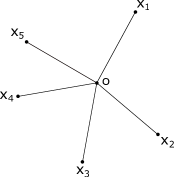
Figure 1. Illustration of $W$ when $X=\{x_{1},\dots,x_{5}\}$.

Clearly, $W$ is a complete $\operatorname{\mathbb{R}}$-tree with internal vertex $o$ and leaves which we identify with $X$. Every complete $\operatorname{\mathbb{R}}$-tree is injective and so, by Lemma 2.1, $\operatorname{\text{\ae}}(X)=\nu(X,W)$.

We set $Y\coloneqq X\cup\{o\}\subset W$. It is easy to check that if $f\colon Y\to E$ is a $1$-Lipschitz map, then the map $\bar{f}\colon W\to E$ which on every edge $[o,x]\subset W$ is given by $w\mapsto(1-t)f(o)+tf(x)$ with $t=d(o,w)/d(o,x)$ is a $1$-Lipschitz extension of $f$. Therefore, $\nu(Y,W)=1$ and we infer $\operatorname{\text{\ae}}(X)=\nu(X,Y)$.

By [5, Theorem 1.1], any $L$-Lipschitz map between complete metric spaces can always be extended to one additional point such that the resulting map is $2L$-Lipschitz. As a result, $\nu(X,Y)\leq 2$, which gives (4.1) when $X$ is infinite.

Suppose now that $X=\{x_{1},\dots,x_{n}\}$ with $n\geq 2$ and consider $x_{1}$ as basepoint. Let $f\colon Y\to\ell_{1}^{n}$ denote the map defined by $f(x_{1})=0$, $f(x_{i})=e_{1}-e_{i}$ for $i=2,\dots,n$ and $f(o)=e_{1}$. Due to Lemma 2.7 the map $\beta_{f}\colon\mathcal{F}(Y)\to\ell_{1}^{n}$ is a linear isometry. By construction, $\beta_{f}(\mathcal{F}(X))=H$, where

$$H\coloneqq\Big{\{}v\in\ell_{1}^{n}:\sum_{i=1}^{n}v_{i}=0\Big{\}},$$

It is a classical fact due to Bohnenblust (see [7, Section 5]) that $\lambda(H,\ell_{1}^{n})=2-2/n$ for all $n\geq 2$. As a result, we obtain $\lambda(\mathcal{F}(X),\mathcal{F}(Y))=2-2/n$. By Lemma 3.1, $\nu(X,Y)=\lambda(\mathcal{F}(X),\mathcal{F}(Y))$, and so, by the above,

$$\operatorname{\text{\ae}}(X)=\nu(X,Y)=\lambda(\mathcal{F}(X),\mathcal{F}(Y))=2-2/n,$$

as desired. ∎

Now we are in position to prove Proposition 1.7.

Proof of Proposition 1.7.

Suppose $\rho(X)\neq\infty$, where

$$\rho(X)\coloneqq\frac{\operatorname{diam}X}{\operatorname{sep}X}.$$

Let $\delta\colon X\times X\to\operatorname{\mathbb{R}}$ denote the metric given by $\delta(x,x^{\prime})\coloneqq\rho(X)$ for all distinct points $x$, $x^{\prime}\in X$. We put $X_{\delta}=(X,\delta)$. The identity map $\operatorname{id}\colon(X,d)\to(X,\delta)$ is $\rho(X)$-bilipschitz. Consequently, using Lemma 2.4, we find

$$\operatorname{\text{\ae}}(X)\leq\rho(X)\operatorname{\text{\ae}}(X_{\delta}).$$ (4.2)

As $\delta$ is a discrete metric, Lemma 4.1 tells us that $\operatorname{\text{\ae}}(X_{\delta})\leq 2-2/\lvert X\rvert$. By combining this inequality with (4.2), we conclude $\operatorname{\text{\ae}}(X)\leq\rho(X)(2-2/\lvert X\rvert)$, as desired. ∎

Next, we proceed with the proof of Proposition 1.5.

Proof of Proposition 1.5.

As pointed out in the introduction, $\operatorname{\text{\ae}}(n)\leq\lambda_{n-1}$. Thus, since $\lambda_{2}=\frac{4}{3}$, as established by Chalmers and Lewicki in [12], it follows that $\operatorname{\text{\ae}}(3)\leq\frac{4}{3}$. Now, Lemma 4.1 tells us that for a three-point metric space $X$ with $d(x,x^{\prime})=1$ for all distinct $x$, $x^{\prime}\in X$, one has $\operatorname{\text{\ae}}(X)=2-\frac{2}{3}=\frac{4}{3}$. This completes the proof. ∎

We are left to establish Proposition 1.6, whose proof is more involved than the previous ones. We follow the proof strategy outlined in Section 1.3. To obtain the upper bound, we need the following proposition:

Proposition 4.2.

For every four-point metric space $X$, there exists a metric space $Y\supset X$ with $\lvert Y\rvert\leq 8$ such that $\operatorname{\text{\ae}}(X)=\nu(X,Y)$.

Proof.

Let $X=\{x_{1},\dots,x_{4}\}$ be a metric space consisting of four points. By relabeling the points if necessary, we can assume that

$$d(x_{1},x_{3})+d(x_{2},x_{4}) \geq d(x_{1},x_{2})+d(x_{3},x_{4}),$$

$$d(x_{1},x_{3})+d(x_{2},x_{4}) \geq d(x_{1},x_{4})+d(x_{2},x_{3}).$$

By a result due to Dress (see [15, Paragraph 1.16]), it follows that the distance matrix of $X$ is of the following form:

$$\begin{pmatrix}0&a+\ell+b&a+\ell+w+c&a+w+d\\ a+\ell+b&0&b+w+c&b+\ell+w+d\\ a+\ell+w+c&b+w+c&0&c+\ell+d\\ a+w+d&b+\ell+w+d&c+\ell+d&0\end{pmatrix},$$ (4.3)

where $a$, $b$, $c$, $d\geq 0$ and $\ell\geq w\geq 0$. Here, the $(i,j)$-th entry of the above matrix is equal to $d(x_{i},x_{j})$. Dress (see [15, Paragraph 1.16]) showed that the injective hull $E(X)$ of $X$ is isometric to the metric space depicted in Figure 2 considered as a subset of $\ell_{1}^{2}=(\operatorname{\mathbb{R}}^{2},\lVert\cdot\rVert_{1})$.

Figure 2. The injective hull $E(X)\subset\ell_{1}^{2}$ of a four-point metric space $X=\{x_{1},\dots,x_{4}\}$ with distance matrix (4.3).

Let $y_{1}\in E(S)\subset\ell_{1}^{2}$ denote the unique point such that $d(x_{1},y_{1})=a$, and define the points $y_{2}$, $y_{3}$, $y_{4}\in E(X)$ analogously. We set $Y\coloneqq X\cup\{y_{1},\dots,y_{4}\}\subset E(X)$.

We claim that $\nu(X,Y)=\operatorname{\text{\ae}}(X)$. As $\operatorname{\text{\ae}}(X)=\nu(X,E(X))$, to establish the claim it suffices to show that $\nu(X,E(X))\leq\nu(X,Y)$. Let $f\colon X\to E$ be a $1$-Lipschitz function to a Banach space $E$ and denote by $\bar{f}\colon Y\to E$ a $K$-Lipschitz extension of $f$ to $Y$, where $K\coloneqq\nu(X,Y)$. We consider $E(X)$ as a subset of $\ell_{1}^{2}$ such that the sides of the rectangle with vertices $y_{i}$ are parallel to the coordinate axes. We define the map $\bar{f}\colon E(X)\to E$ as follows:

• If $y=(1-t)x_{i}+ty_{i}$ for some $t\in[0,1]$, then we set

  $$\bar{f}(y)\coloneqq(1-t)\bar{f}(x_{i})+t\bar{f}(y_{i}).$$

• If $y=\alpha_{1}y_{1}+\alpha_{2}y_{2}+\alpha_{3}y_{3}$ with $\alpha_{i}\geq 0$ and $\alpha_{1}+\alpha_{2}+\alpha_{3}=1$, then we set

  $$\bar{f}(y)\coloneqq\alpha_{1}\bar{f}(y_{1})+\alpha_{2}\bar{f}(y_{2})+\alpha_{3}\bar{f}(y_{3}).$$

• If $y=\beta_{1}y_{1}+\beta_{3}y_{3}+\beta_{4}y_{4}$ with $\beta_{i}\geq 0$ and $\beta_{1}+\beta_{3}+\beta_{4}=1$, then we set

  $$\bar{f}(y)\coloneqq\beta_{1}\bar{f}(y_{1})+\beta_{3}\bar{f}(y_{3})+\beta_{4}\bar{f}(y_{4}).$$

The map $\bar{f}$ is well-defined and an extension of $f$. In the following, we show that $f$ is $K$-Lipschitz. Notice that if $y=\beta_{1}y_{1}+\beta_{3}y_{3}+\beta_{4}y_{4}$ and $y^{\prime}=\beta_{1}^{\prime}y_{1}+\beta_{3}^{\prime}y_{3}+\beta_{4}^{\prime}y_{4}$, then

$$y-y^{\prime}=(\beta_{1}-\beta_{1}^{\prime})(y_{1}-y_{4})+(\beta_{3}-\beta_{3}^{\prime})(y_{3}-y_{4})$$

and therefore

$$d(y,y^{\prime})=\lVert y-y^{\prime}\rVert_{1}=\lvert\beta_{1}-\beta_{1}^{\prime}\rvert w+\lvert\beta_{3}-\beta_{3}^{\prime}\rvert\ell.$$ (4.4)

Clearly,

$$\lVert\bar{f}(y)-\bar{f}(y^{\prime})\rVert\leq\lvert\beta_{1}-\beta_{1}^{\prime}\rvert\,\,\lVert\bar{f}(y_{1})-\bar{f}(y_{4})\rVert+\lvert\beta_{3}-\beta_{3}^{\prime}\rvert\,\,\lVert\bar{f}(y_{3})-\bar{f}(y_{4})\rVert;$$

hence, by virtue of (4.4), we have $\lVert\bar{f}(y)-\bar{f}(y^{\prime})\rVert\leq Kd(y,y^{\prime})$ for all points $y$, $y^{\prime}$ contained in the convex hull of $y_{1},y_{3},y_{4}$.

Analogously, we find that $\bar{f}$ is $K$-Lipschitz on the convex hull of the points $y_{1},y_{2},y_{3}$. A straightforward computation shows that $\bar{f}$ is $K$-Lipschitz on $E(X)$, as desired. Since $f$ and $E$ were arbitrary, it follows that $\nu(X,E(X))\leq\nu(X,Y)$, as was to be shown. ∎

Finally, we give the proof of Proposition 1.6.

Proof of Proposition 1.6.

Let $X$ be any four-point metric space. By Proposition 4.2, there exists a metric space $Y\supset X$ such that $\lvert Y\rvert\leq 8$ and $\operatorname{\text{\ae}}(X)=\nu(X,Y)$. Lemma 3.1 tells us that $\nu(X,Y)=\lambda(\mathcal{F}(X),\mathcal{F}(Y))$. Consequently, as $\dim\mathcal{F}(X)=3$ and $\dim\mathcal{F}(Y)\leq 7$, we have $\operatorname{\text{\ae}}(X)\leq\bar{\lambda}(3,7)$, where $\bar{\lambda}(n,d)$ is defined as in (1.12). Using the upper bound (1.13), we arrive at

$$\operatorname{\text{\ae}}(4)\leq\frac{3+6\sqrt{2}}{7},$$

as desired. Next, we deal with the lower bound. We abbreviate

$$\alpha\coloneqq\frac{1}{\sqrt{2}}+\frac{1}{2}\quad\text{ and }\quad\beta\coloneqq\frac{1}{\sqrt{2}}-\frac{1}{2}.$$

We define the points $x_{1},x_{2},x_{3},x_{4},y_{1},y_{2}\in\ell^{2}_{\infty}$ as follows:

$$x_{1} \coloneqq(-\alpha,-1), x_{2} \coloneqq(-\alpha,1), x_{3} \coloneqq(\alpha,1), x_{4} \coloneqq(\alpha,-1),$$

$$y_{1} \coloneqq(-\beta,0), y_{2} \coloneqq(\beta,0).$$

The points $x_{1},\dots,x_{4}$ are the vertices of a rectangle with side lengths $2$ and $\sqrt{2}+1$. We set $X\coloneqq\{x_{1},\dots,x_{4}\}\subset\ell_{\infty}^{2}$ and $Y\coloneqq X\cup\{y_{1},y_{2}\}\subset\ell_{\infty}^{2}$. By Theorem 1.4,

$$\operatorname{\text{\ae}}(X)\geq\lambda(\mathcal{F}(X),\mathcal{F}(Y)).$$

In the following, we show that $\lambda(\mathcal{F}(X),\mathcal{F}(Y))\geq(5+4\sqrt{2})/7$. Let $T=(Y,E)$ denote the graph with vertex set $Y$ and edge set $E=\{f_{1},\dots,f_{5}\}$, where

$$f_{1} \coloneqq\{x_{1},y_{1}\}, f_{2} \coloneqq\{x_{2},y_{1}\}, f_{3} =\{y_{1},y_{2}\},$$

$$f_{4} \coloneqq\{y_{2},x_{3}\}, f_{5} \coloneqq\{y_{2},x_{4}\}.$$

By construction, $T$ is a tree, and every $x_{i}$ is a leaf of $T$ and $y_{1}$ and $y_{2}$ are internal vertices of degree 3. Let $d_{T}$ denote shortest-path metric on $T$ induced by the weight function $\omega\colon E\to(0,\infty)$ defined by $\omega(\{x,y\})\coloneqq d(x,y)$. The identity map $\operatorname{id}\colon(Y,d)\to(T,d_{T})$ is an isometry. Fix $x_{1}$ as a basepoint. Clearly, $B=\{b_{1},\dots,b_{5}\}$ with $b_{i}=\delta(x_{i+1})$, for $i=1,2,3$, and $b_{i}=\delta(y_{i-3})$, for $i=4,5$, is a basis of $\mathcal{F}(T)$. Using this basis, let $L\colon\mathcal{F}(T)\to\ell_{1}^{5}$ denote the linear map induced by the matrix

$$M\coloneqq\left[\begin{array}[]{ccccc}1&1&1&1&1\\ 1&0&0&0&0\\ 0&\gamma&\gamma&0&\gamma\\ 0&1&0&0&0\\ 0&0&1&0&0\\ \end{array}\right],$$

where $\gamma\coloneqq\sqrt{2}-1$. Notice that the map $f\colon T\to\ell_{1}^{5}$ defined by $f\coloneqq L\circ\delta$ satisfies the assumptions of Lemma 2.7. Consequently, as $L=\beta_{f}$, which is due to the uniqueness of $\beta_{f}$, it follows from Lemma 2.7 that $L$ is a linear isometry.

Let $v_{i}\in\ell_{1}^{5}$ denote the $i$th column of the matrix $M$. By definition of $L$, one has $L(\mathcal{F}(X))=E$, where $E\subset\ell_{1}^{5}$ is the linear span of the vectors $v_{1}$, $v_{2}$ and $v_{3}$. Hence, as $L$ is a linear isometry, $\lambda(\mathcal{F}(X),\mathcal{F}(Y))=\lambda(E,\ell_{1}^{5})$. We set

$$S\coloneqq\left[\begin{array}[]{ccccc}1&1&1&1&1\\ 1&1&-1&-1&-1\\ 1&-1&1&1&1\\ 1&-1&1&1&-1\\ 1&-1&1&-1&1\\ \end{array}\right]$$ (4.5)

and denote by $D\in\mathcal{M}_{5}(\operatorname{\mathbb{R}})$ the diagonal matrix with diagonal $(\nu,\nu,\mu,\nu,\nu)$, where $\mu\coloneqq(5-3\sqrt{2})/7$ and $\nu\coloneqq(1-\mu)/4$. Via a direct computation, one can show that $u_{1}\coloneqq v_{2}+v_{3}-v_{1}$ is an eigenvector of $DS$ with eigenvalue $\lambda_{1}\coloneqq(\sqrt{2}+3)/7$, and the independent vectors $u_{2}\coloneqq v_{3}-v_{2}$ and $u_{3}\coloneqq v_{1}$, are eigenvectors of $DS$ with eigenvalues $\lambda_{2}=\lambda_{3}\coloneqq(3\sqrt{2}+2)/14$.

Since $u_{1},u_{2},u_{3}$ is a basis of $E$, we find that $AP=PAP$, where $A\coloneqq DS$ and $P\colon\ell_{1}^{5}\to E$ denotes the transformation matrix of the orthogonal projection from $\operatorname{\mathbb{R}}^{5}$ onto $E\subset\operatorname{\mathbb{R}}^{5}$. Notice that $\operatorname{tr}(D)=1$ and thus, by (5.1), it follows that $\nu_{1}(A)=1$. By Proposition 5.2,

$$\lambda(E,\ell_{1}^{5})\geq\operatorname{tr}(AP)=\sum_{i=1}^{3}\frac{1}{\lVert u_{i}\rVert^{2}_{2}}\operatorname{tr}(Au_{i}u_{i}^{T})=\sum_{i=1}^{3}\lambda_{i}=\frac{5+4\sqrt{2}}{7},$$

where we have used that the vectors $u_{i}$ are orthogonal to each other. Using the identity $\lambda(\mathcal{F}(X),\mathcal{F}(Y))=\lambda(E,\ell_{1}^{5})$, we conclude that

$$\operatorname{\text{\ae}}(4)\geq\operatorname{\text{\ae}}(X)\geq\lambda(\mathcal{F}(X),\mathcal{F}(Y))\geq\frac{5+4\sqrt{2}}{7}.$$

This completes the proof. ∎

Remark 4.3.

Given a matrix $A$, the matrix $\textrm{Sgn}(A)=(b_{ij})$ defined by $b_{ij}\coloneqq\operatorname{sgn}(a_{ij})$ is called sign pattern matrix of $A$. The matrix $S$ appearing in the proof of Proposition 1.6 is the sign pattern matrix of the matrix $P$. In general, given a linear projection $P\colon\ell_{1}^{d}\to E$, good candidates for a matrix $A\in\mathcal{M}_{d}(\operatorname{\mathbb{R}})$ with $\operatorname{tr}(AP)=\lambda(E,\ell_{1}^{d})$ are matrices of the form $A=D\textrm{Sgn}(P)$, where $D$ is a diagonal matrix with positive entries.

5. Projection constants and linear programming

5.1. Banach space theory

In the following, we recall standard concepts from Banach space theory. For each integer $d\geq 1$ let $\mathcal{M}_{d}(\mathbb{R})$ denote the real vector space of all $d\times d$ matrices with real entries. For every linear map $f\colon\mathcal{M}_{d}(\mathbb{R})\to\operatorname{\mathbb{R}}$ there exists a unique matrix $A\in\mathcal{M}_{d}(\mathbb{R})$ such that

$$f(X)=\operatorname{tr}(AX)\quad\text{ for all }X\in\mathcal{M}_{d}(\mathbb{R}).$$

For every Banach space $E=(\operatorname{\mathbb{R}}^{d},\lVert\cdot\rVert_{{}_{E}})$ we let $\mathcal{L}(E)=(\mathcal{M}_{d}(\operatorname{\mathbb{R}}),\lVert\cdot\rVert_{\mathcal{L}(E)})$ denote Banach space of all linear operators from $E$ to $E$ equipped with the operator norm $\lVert\cdot\rVert_{\mathcal{L}(E)}$. The $1$-nuclear norm $\nu_{1}(A)$ of $A\in\mathcal{L}(E)$ is defined as follows

$$\nu_{1}(A)\coloneqq\inf\Big{\{}\sum_{i=1}^{m}\lVert f_{i}\rVert_{{}_{E^{\ast}}}\lVert x_{i}\rVert_{{}_{E}}:m\geq 1,A=\sum_{i=1}^{m}f_{i}\otimes x_{i}\Big{\}}.$$

It is well-known that the dual space of $\mathcal{L}(E)$ can be identified with $(\mathcal{M}_{d}(\operatorname{\mathbb{R}}),\nu_{1}(\cdot))$, and so

$$\nu_{1}(A)=\max\big{\{}\operatorname{tr}(AX)\,:\,X\in\mathcal{M}_{d}(\mathbb{R})\textrm{ with }\lVert X\rVert_{\mathcal{L}(E)}=1\big{\}}$$

for all $A\in\mathcal{M}_{d}(\operatorname{\mathbb{R}})$. If $E=\ell_{1}^{d}$, then

$$\nu_{1}(A)=\sum_{i=1}^{d}\max_{j}\,\lvert a_{ij}\rvert$$ (5.1)

for all $A\in\mathcal{M}_{d}(\operatorname{\mathbb{R}})$.

Given a Banach space $E$, we denote by $\operatorname{ext}B_{E}$ the set of extreme points of the closed unit ball $B_{E}$ of $E$. A finite-dimensional Banach space $E$ is said to be polyhedral, if $\operatorname{ext}B_{E^{\ast}}$ is finite. If $E$ is polyhedral and $S\coloneqq\{f_{1},\dots,f_{d}\}\subset\operatorname{ext}B_{E^{\ast}}$ is a subset such $S\cup-S=\operatorname{ext}B_{E^{\ast}}$ and $\lvert\operatorname{ext}B_{E^{\ast}}\rvert=2d$, then $\alpha\colon E\hookrightarrow\ell_{\infty}^{d}$ defined by $x\mapsto(f_{i}(x))$ is a linear isometric embedding. Conversely, every finite-dimensional linear subspace of $\ell_{\infty}^{d}$ is polyhedral. If $F=(\operatorname{\mathbb{R}}^{d},\lVert\cdot\rVert_{{}_{F}})$ is a polyhedral Banach space, then $\mathcal{L}(F)$ is polyhedral as well. In fact, $\operatorname{ext}B_{\mathcal{L}(F)^{\ast}}$ is equal to $\operatorname{ext}B_{F^{\ast}}\otimes\operatorname{ext}B_{F}$ (see [36]).

5.2. Computation of projection constants via linear programming

The aim of this section is to establish a characterization of $\lambda(E,F)$ as the optimal value of a certain linear programming problem (see Lemma 5.1).

Let $F=(\operatorname{\mathbb{R}}^{d},\lVert\cdot\rVert_{F})$ be a polyhedral Banach space and $E\subset F$ a nontrivial linear subspace that is not equal to $F$. Suppose that $u_{r}\in\operatorname{\mathbb{R}}^{d}$, $r=1,\dots,n$, is an orthonormal basis of $E\subset\operatorname{\mathbb{R}}^{d}$ and $v_{s}\in\operatorname{\mathbb{R}}^{d}$, $s=1,\dots,d-n$, an orthonormal basis of its orthogonal complement. Fix an enumeration $\{B_{1},\dots,B_{p}\}$ of

$$\big{\{}u_{r^{\phantom{1}}}u_{r^{\prime}}^{T}\big{\}}\cup\big{\{}v_{{s^{\phantom{1}}}}v_{s^{\prime}}^{T}\big{\}}\cup\big{\{}u_{r^{\phantom{1}}}v_{s}^{T}\big{\}}$$

such that $B_{i}=u_{i}u_{i}^{T}$ for all $i=1,\dots,n$ and fix an enumeration $\{E_{1},\dots,E_{q}\}$ of the extreme points of the closed unit ball of $\mathcal{L}(F)$.

Lemma 5.1.

We define the matrix $A\in\mathcal{M}_{p\times q}(\operatorname{\mathbb{R}})$ via $a_{ij}=\operatorname{tr}(B_{i}E_{j})$ and the vector $b\in\operatorname{\mathbb{R}}^{p}$ by setting $b_{i}=1$ for all $i=1,\dots,n$ and $b_{i}=0$ otherwise. Let $j\in\operatorname{\mathbb{R}}^{q}$ denote the all-ones vector. Then the linear programming problem

$$\text{minimize}\quad j^{T}x$$

$$\text{subject to}\quad Ax =b$$

$$x \geq 0$$

is solvable and its optimal value is equal to $\lambda(E,F)$.

We suggest the book [29] for an introduction to linear programming. A few remarks are in order.

• Lemma 5.1 is particularly useful when $F=\ell_{\infty}^{d}$. In this case $\lambda(E,F)=\lambda(E)$ for every subspace $E\subset F$. This is a direct consequence of the fact that $\ell_{\infty}^{d}$ is an injective Banach space for every $d\geq 1$.

• In the special case when $F=\ell_{\infty}^{d}$, the set of extreme points $\operatorname{ext}B_{\mathcal{L}(F)}$ can be characterized as follows: $M\in\mathcal{M}_{d}(\operatorname{\mathbb{R}})$ is contained in $\operatorname{ext}B_{\mathcal{L}(F)}$ if and only if for each $i\in\{1,\dots,d\}$ there exists a unique $j\in\{1,\dots,d\}$ such that $\lvert m_{ij}\rvert=1$ and $m_{ik}=0$ for all $k\neq j$. Hence, the set $\operatorname{ext}B_{\mathcal{L}(\ell_{\infty}^{d})}$ contains exactly $2^{d+1}d^{d}$ matrices.

• For an arbitrary polyhedral Banach space $F$, computing the extreme points of the closed unit ball of $\mathcal{L}(F)$ is not an easy task. Since $\operatorname{ext}B_{\mathcal{L}(F)^{\ast}}=\operatorname{ext}B_{F^{\ast}}\otimes\,\operatorname{ext}B_{F}$, the $V$-representation of the convex polytope

  $$\mathcal{P}\coloneqq B_{\mathcal{L}(F)^{\ast}}\subset\mathcal{M}_{d}(\operatorname{\mathbb{R}})$$

  is known, and a general strategy for determining $\operatorname{ext}B_{\mathcal{L}(F)}$ is to compute the $H$-representation of $\mathcal{P}$.

The following formula for $\lambda(E,F)$ is essentially known (see [24, Lemma 1]). For the convenience of the reader, we give an elementary and detailed proof of it at the end of the subsection.

Proposition 5.2.

Let $F=(\operatorname{\mathbb{R}}^{d},\lVert\cdot\rVert)$ be a polyhedral Banach space and $E\subset F$ a linear subspace. Then

$$\lambda(E,F)=\max\big{\{}\operatorname{tr}(AP):A\in\mathcal{M}_{d}(\mathbb{R}),\,\nu_{1}(A)=1\textrm{ and }AP=PAP\,\big{\}},$$ (5.2)

where $P\in\mathcal{M}_{d}(\operatorname{\mathbb{R}})$ is the transformation matrix of the orthogonal projection from $\operatorname{\mathbb{R}}^{d}$ onto $E\subset\operatorname{\mathbb{R}}^{d}$.

Now, Lemma 5.1 follows from the proposition above and the strong duality theorem of linear programming.

Proof of Lemma 5.1.

Notice that $B\in\mathcal{M}_{d}(\operatorname{\mathbb{R}})$ satisfies $BP=PBP$ if and only if

$$B=\sum_{i=1}^{p}x_{i}B_{i}$$

for some real numbers $x_{1},\dots,x_{p}\in\operatorname{\mathbb{R}}$. For any such matrix $B$ we have

$$\operatorname{tr}(BP)=\langle b,x\rangle_{\operatorname{\mathbb{R}}^{p}}=b^{T}x,$$

where $x\coloneqq(x_{1},\dots,x_{p})$. Further, notice that $\nu_{1}(B)\leq 1$ if and only if $A^{T}x\leq j$. Hence, using Proposition 5.2, we find that the optimal value of the linear programming problem

$$\text{maximize}\quad b^{T}x$$

$$\text{subject to}\quad A^{T}x \leq j$$

is equal to $\lambda(E,F)$. Now, the conclusion of the lemma follows directly from the strong duality theorem of linear programming (see, for example, [29, p. 85]). ∎

Proof of Proposition 5.2.

Let $A\in\mathcal{M}_{d}(\mathbb{R})$ be such that $AP=PAP$ and let $Q\in\mathcal{M}_{d}(\mathbb{R})$ be a projection matrix with range $E$. We compute

$$\begin{split}\operatorname{tr}(AP)&=\operatorname{tr}(AQP)=\operatorname{tr}(PAQ)\\ &=\operatorname{tr}(PAPQ)=\operatorname{tr}(APQ)=\operatorname{tr}(AQ)\leq\nu_{1}(A)\,\lVert Q\rVert_{\mathcal{L}(F)}.\end{split}$$

Hence, the left hand side of (5.2) is greater than or equal to the right hand side. In the following, we establish the other inequality.

Clearly, (5.2) is true if $E=\{0\}$ or $E=F$, therefore we may suppose that $\dim(E)\neq 0,d$. Let $u_{r}\in\operatorname{\mathbb{R}}^{d}$, $r=1,\dots,n$, be an orthonormal basis of $E\subset\operatorname{\mathbb{R}}^{d}$ and $v_{s}\in\operatorname{\mathbb{R}}^{d}$, $s=1,\dots,d-n$, an orthonormal basis of its orthogonal complement. Every matrix contained in the set $P+H$, where $H$ is the linear span of $\big{\{}u_{r^{\phantom{1}}}v_{s}^{T}\big{\}}$, is a projection matrix with range $E$. Let $\textrm{Proj}\subset\mathcal{M}_{d}(\mathbb{R})$ denote the linear span of $P+H$ and fix a decomposition $\mathcal{M}_{d}(\mathbb{R})=\textrm{Proj}\oplus\textrm{Aux}$, where $\textrm{Aux}\subset\mathcal{M}_{d}(\mathbb{R})$ is a linear subspace. We set

$$\textrm{Proj}^{\ast}\coloneqq\big{\{}A\in\mathcal{M}_{d}(\mathbb{R}):\operatorname{tr}(AX)=0\textrm{ for all }X\in\textrm{Aux}\big{\}}.$$

We claim that there exists $A\in\textrm{Proj}^{\ast}$, $A\neq 0$, such that $AP=PAP$.

The linear map $L\colon\mathcal{M}_{d}(\mathbb{R})\to\mathcal{M}_{d}(\mathbb{R})$ defined by $X\mapsto XP-PXP$ satisfies $L|_{W_{0}}=0$ and $L|_{W_{1}}=\textrm{id}|_{W_{1}}$, where $W_{0}\subset\mathcal{M}_{d}(\mathbb{R})$ is the linear span of the matrices $\big{\{}u_{r^{\phantom{1}}}u_{r^{\prime}}^{T}\big{\}},\big{\{}v_{{s^{\phantom{1}}}}v_{s^{\prime}}^{T}\big{\}}\textrm{ and }\big{\{}u_{r^{\phantom{1}}}v_{s}^{T}\big{\}}$ and $W_{1}\subset\mathcal{M}_{d}(\mathbb{R})$ the linear span of the matrices $\{v_{s^{\phantom{1}}}u_{r}^{T}\}$. Hence, the kernel of $L$ has dimension $d^{2}-n(d-n)$, and since the dimension of $\textrm{Proj}^{\ast}\subset\mathcal{M}_{d}(\mathbb{R})$ is equal to $n(d-n)+1$, the matrix $A$ with the desired properties exists.

Now, fix $A\in\textrm{Proj}^{\ast}\cap W_{0}$, $A\neq 0$, and define the linear map $f_{A}\colon\textrm{Proj}\to\operatorname{\mathbb{R}}$ via $X\mapsto\operatorname{tr}(AX)$. As $A\in\textrm{Proj}^{\ast}$ and $A\neq 0$, it follows that $f_{A}\neq 0$. In the following, we consider Proj as a linear subspace of $\mathcal{L}(F)$ equipped with the induced norm. Clearly, there exists a matrix $B\in\textrm{Proj}$ such that $\lVert B\rVert=1$ and $\lVert f_{A}\rVert=f_{A}(B)$. In particular, $f_{A}(B)\neq 0$.

As $AP=PAP$, it follows that $Ax\in E$ for all $x\in E$, which is in fact equivalent to $AP=PAP$. Consequently,

$$\operatorname{tr}(A\hskip 1.00006ptu_{r^{\phantom{1}}}v_{s}^{T})=\langle Au_{r},v_{s}\rangle_{\operatorname{\mathbb{R}}^{d}}=0$$ (5.3)

for all $r=1,\dots,n$ and all $s=1,\dots,d-n$. This implies that $\operatorname{tr}(AX)=0$ for all $X\in H$. Hence, as $f_{A}(B)\neq 0$, there is a projection matrix $Q\in P+H$ and a scalar $\alpha\neq 0$ such that $B=\alpha Q$. Notice that $\lVert f_{A}\rVert=\alpha\operatorname{tr}(AQ)$ and $1=\lVert B\rVert=\lvert\alpha\rvert\cdot\lVert Q\rVert$. Therefore,

$$\lVert Q\rVert=\operatorname{tr}\Bigl{(}\tfrac{\operatorname{sgn}(\alpha)}{\lVert f_{A}\rVert}\,AQ\Bigr{)},$$

where $\operatorname{sgn}(\alpha)$ denotes the sign of $\alpha$.

By the Hahn-Banach theorem there is a linear functional $\bar{f}_{A}\colon\mathcal{L}(F)\to\operatorname{\mathbb{R}}$ extending $f_{A}$ such that $\lVert\bar{f}_{A}\rVert=\lVert f_{A}\rVert$. Hence, by trace duality there exists $\bar{A}\in\mathcal{M}_{d}(\mathbb{R})$ such that $\bar{f}_{A}(X)=\operatorname{tr}(\bar{A}X)$ for all $X\in\mathcal{M}_{d}(\mathbb{R})$. Clearly, $\nu_{1}(\bar{A})=\lVert\bar{f}_{A}\rVert$ and $\operatorname{tr}(\bar{A}X)=\operatorname{tr}(AX)$ for all $X\in\textrm{Proj}$. Using (5.3), we find that $\langle\bar{A}u_{r},v_{s}\rangle_{\operatorname{\mathbb{R}}^{d}}=0$; this implies that $\bar{A}x\in E$ for all $x\in E$ and thus $\bar{A}P=P\bar{A}P$.

Letting $A_{0}\coloneqq\bigl{(}\operatorname{sgn}(\alpha)/\nu_{1}(\bar{A})\bigr{)}\,\bar{A}$, it follows by the above that $\lVert Q\rVert=\operatorname{tr}(A_{0}Q)$ and $A_{0}P=PA_{0}P$. Hence, using that $\operatorname{tr}(A_{0}P)=\operatorname{tr}(A_{0}Q)$ and $\lVert Q\rVert\geq\lambda(E,F)$, we conclude $\operatorname{tr}(A_{0}P)\geq\lambda(E,F)$, as desired. This completes the proof. ∎

References

- [1] Richard F. Arens and James Eells “On embedding uniform and topological spaces” In Pacific J. Math. 6, 1956, pp. 397–403 URL: http://projecteuclid.org/euclid.pjm/1103043959
- [2] Keith Ball “Markov chains, Riesz transforms and Lipschitz maps” In Geometric & Functional Analysis GAFA 2.2 Springer, 1992, pp. 137–172
- [3] Giuliano Basso “Computation of maximal projection constants” In J. Funct. Anal. 277.10, 2019, pp. 3560–3585 DOI: 10.1016/j.jfa.2019.05.011
- [4] Giuliano Basso “Fixed point and Lipschitz extension theorems for barycentric metric spaces” Zurich: ETH Zurich, 2019-12 DOI: 10.3929/ethz-b-000398970
- [5] Giuliano Basso “Lipschitz extensions to finitely many points” In Anal. Geom. Metr. Spaces 6.1, 2018, pp. 174–191 DOI: 10.1515/agms-2018-0010
- [6] Giuliano Basso and Hubert Sidler “Approximating spaces of Nagata dimension zero by weighted trees” In arXiv: 2104.13674, 2021
- [7] .F Bohnenblust “Convex regions and projections in Minkowski spaces” In Annals of Mathematics JSTOR, 1938, pp. 301–308
- [8] A. Brudnyi and Y. Brudnyi “Linear and nonlinear extensions of Lipschitz functions from subsets of metric spaces” In Algebra i Analiz 19.3, 2007, pp. 106–118 DOI: 10.1090/S1061-0022-08-01003-0
- [9] Alexander Brudnyi and Yuri Brudnyi “Methods of geometric analysis in extension and trace problems. Volume 1” 102, Monographs in Mathematics Birkhäuser/Springer Basel AG, Basel, 2012, pp. xxiv+560
- [10] Alexander Brudnyi and Yuri Brudnyi “Methods of geometric analysis in extension and trace problems. Volume 2” 103, Monographs in Mathematics Birkhäuser/Springer Basel AG, Basel, 2012, pp. xx+414
- [11] Alexander Brudnyi and Yuri Brudnyi “Metric spaces with linear extensions preserving Lipschitz condition” In Amer. J. Math. 129.1, 2007, pp. 217–314 DOI: 10.1353/ajm.2007.0000
- [12] Bruce L. Chalmers and Grzegorz Lewicki “A proof of the Grünbaum conjecture” In Studia Mathematica 200.2, 2010, pp. 103–129 URL: http://eudml.org/doc/285668
- [13] Bruce L. Chalmers and Grzegorz Lewicki “Three-dimensional subspace of with maximal projection constant” In Journal of Functional Analysis 257.2, 2009, pp. 553 –592 DOI: https://doi.org/10.1016/j.jfa.2009.01.005
- [14] Stefan Cobzaş, Radu Miculescu and Adriana Nicolae “Lipschitz functions” 2241, Lecture Notes in Mathematics Springer, Cham, 2019, pp. xiv+591 DOI: 10.1007/978-3-030-16489-8
- [15] Andreas W. M. Dress “Trees, tight extensions of metric spaces, and the cohomological dimension of certain groups: a note on combinatorial properties of metric spaces” In Adv. in Math. 53.3, 1984, pp. 321–402 DOI: 10.1016/0001-8708(84)90029-X
- [16] S. Foucart and L. Skrzypek “On maximal relative projection constants” In J. Math. Anal. Appl. 447.1, 2017, pp. 309–328 DOI: 10.1016/j.jmaa.2016.09.066
- [17] A. Godard “Tree metrics and their Lipschitz-free spaces” In Proc. Amer. Math. Soc. 138.12, 2010, pp. 4311–4320 DOI: 10.1090/S0002-9939-2010-10421-5
- [18] G. Godefroy and N. J. Kalton “Lipschitz-free Banach spaces” In Studia Math. 159.1, 2003, pp. 121–141 DOI: 10.4064/sm159-1-6
- [19] Branko Grünbaum “Projection constants” In Transactions of the American Mathematical Society 95.3 JSTOR, 1960, pp. 451–465
- [20] John R. Isbell “Six theorems about injective metric spaces.” In Commentarii mathematici Helvetici 39, 1964/65, pp. 65–76 URL: http://eudml.org/doc/139281
- [21] G. J. O. Jameson “Summing and nuclear norms in Banach space theory” 8, London Mathematical Society Student Texts Cambridge University Press, Cambridge, 1987, pp. xii+174 DOI: 10.1017/CBO9780511569166
- [22] William B. Johnson, Joram Lindenstrauss and Gideon Schechtman “Extensions of Lipschitz maps into Banach spaces” In Israel J. Math. 54.2, 1986, pp. 129–138 DOI: 10.1007/BF02764938
- [23] M. Ĭ. Kadets and M. G. Snobar “Certain functionals on the Minkowski compactum” In Mat. Zametki 10, 1971, pp. 453–457
- [24] H. König, D. Lewis and P.-K. Lin “Finite dimensional projection constants” In Studia Mathematica 3.75, 1983, pp. 341–358
- [25] Hermann König “Spaces with large projection constants” In Israel Journal of Mathematics 50.3, 1985, pp. 181–188 DOI: 10.1007/BF02761398
- [26] Urs Lang “Injective hulls of certain discrete metric spaces and groups” In Journal of Topology and Analysis 5.03 World Scientific, 2013, pp. 297–331
- [27] James R Lee and Assaf Naor “Extending Lipschitz functions via random metric partitions” In Inventiones mathematicae 160.1 Springer, 2005, pp. 59–95
- [28] Joram Lindenstrauss “On nonlinear projections in Banach spaces.” In Michigan Math. J. 11.3 University of Michigan, Department of Mathematics, 1964, pp. 263–287 DOI: 10.1307/mmj/1028999141
- [29] Jiri Matousek and Bernd Gärtner “Understanding and using linear programming” Springer Science & Business Media, 2007
- [30] Manor Mendel and Assaf Naor “Spectral calculus and Lipschitz extension for barycentric metric spaces” In Anal. Geom. Metr. Spaces 1, 2013, pp. 163–199 DOI: 10.2478/agms-2013-0003
- [31] Assaf Naor “Probabilistic clustering of high dimensional norms” In Proceedings of the Twenty-Eighth Annual ACM-SIAM Symposium on Discrete Algorithms SIAM, Philadelphia, PA, 2017, pp. 690–709 DOI: 10.1137/1.9781611974782.44
- [32] Assaf Naor and Yuval Rabani “On Lipschitz extension from finite subsets” In Israel Journal of Mathematics 219.1 Springer, 2017, pp. 115–161
- [33] Assaf Naor and Lior Silberman “Poincaré inequalities, embeddings, and wild groups” In Compos. Math. 147.5, 2011, pp. 1546–1572 DOI: 10.1112/S0010437X11005343
- [34] Mikhail I. Ostrovskii “Metric embeddings” Bilipschitz and coarse embeddings into Banach spaces 49, De Gruyter Studies in Mathematics De Gruyter, Berlin, 2013, pp. xii+372 DOI: 10.1515/9783110264012
- [35] Albrecht Pietsch “History of Banach spaces and linear operators” Birkhäuser Boston, 2007, pp. xxiv+855
- [36] Wolfgang M. Ruess and Charles P. Stegall “Extreme points in duals of operator spaces” In Math. Ann. 261.4, 1982, pp. 535–546 DOI: 10.1007/BF01457455
- [37] Nicole Tomczak-Jaegermann “Banach-Mazur distances and finite-dimensional operator ideals” 38, Pitman Monographs and Surveys in Pure and Applied Mathematics Longman Scientific & Technical, 1989, pp. xii+395
- [38] Nik Weaver “Lipschitz Algebras” WORLD SCIENTIFIC, 2018 DOI: 10.1142/9911
- [39] P. Wojtaszczyk “Banach spaces for analysts” 25, Cambridge Studies in Advanced Mathematics Cambridge University Press, Cambridge, 1991, pp. xiv+382 DOI: 10.1017/CBO9780511608735