Interferences in the Stochastic Gravitational Wave Background

Abstract

Although the expansion of the Universe explicitly breaks the time-translation symmetry, cosmological predictions for the stochastic gravitational wave background (SGWB) are usually derived under the so-called stationary hypothesis. By dropping this assumption and keeping track of the time dependence of gravitational waves at all length scales, we derive the expected unequal-time (and equal-time) waveform of the SGWB generated by scaling sources, such as cosmic defects. For extinct and smooth enough sources, we show that all observable quantities are uniquely and analytically determined by the holomorphic Fourier transform of the anisotropic stress correlator. Both the strain power spectrum and the energy density parameter are shown to have an oscillatory fine structure, they significantly differ on large scales while running in phase opposition at large wavenumbers $k$. We then discuss scaling sources that are never extinct nor smooth and which generate a singular Fourier transform of the anisotropic stress correlator. For these, we find the appearance of interferences on top of the above-mentioned fine-structure as well as atypical behaviour at small scales. For instance, we expect the rescaled strain power spectrum $k^{2}\mathcal{P}_{h}$ generated by long cosmic strings in the matter era to oscillate around a scale invariant plateau. These singular sources are also shown to produce orders of magnitude difference between the rescaled strain spectra and the energy density parameter suggesting that only the former should be used for making reliable observable predictions. Finally, we discuss how measuring such a fine structure in the SGWB could disambiguate the possible cosmological sources.

1 Introduction

The statistical homogeneity and isotropy of the Universe imply that all gravitational wave sources of natural origin must collectively contribute to the generation of a stochastic background. All types of merger discovered so far by the LIGO-Virgo-Kagra experiments guarantee the existence of a background of astrophysical origin, which is actively searched for [1, 2, 3, 4, 5]. The other possible mechanisms to generate a SGWB are of cosmological origin. Because all astrophysical sources fade away above some redshift, it is very well possible that the first detection of a SGWB could be of cosmological origin thereby providing unexpected discoveries (see, e.g., Refs. [6, 7, 8] for reviews).

In fact, this possibility has long been considered [9, 10, 11, 12, 13, 14, 15, 16, 17]. For instance, measuring the effective number of relativistic degrees of freedom in the cosmic plasma gives an upper limit to the amplitude of the (sub-Hubble) SGWB at the time of recombination [18], and also as early as during Big-Bang Nucleosynthesis (BBN) [19, 20]. These types of constraint are derived from the changes in the expansion rate of the Universe induced by the overall gravitating effect of gravitational waves. As such, they are sensitive to their integrated “energy” and the constraints are given in terms of the so-called energy density parameter $\Omega_{\mathrm{gw}}$. Other detection channels in cosmology exist as well. The $B$-mode polarisation of the Cosmic Microwave Background (CMB) anisotropies is sensitive to spin one and spin two metric fluctuations and it can be used to constrain gravitational waves [21, 22]. Observational bounds are given on the amplitude of the primordial (strain) power spectrum $\mathcal{P}_{h}(k)$, at a given wavenumber [23, 24]. Here $k$ is the wavenumber associated with a spatial Fourier transform. Interferometers, and pulsar arrays, are also sensitive to the strain of a passing GW, and the measurable quantity is the so-called strain power spectral density $S_{h}(\omega)$ [25]. Here $\omega$ is the angular frequency associated with a temporal Fourier transform. Both approaches are rooted in what is measurable within a given apparatus. Apart from the Earth’s and Solar System’s motion, direct detection experiments assume measurements to be done at a fixed location. The parameter against which measurements are made, and stochasticity can be inferred, is the time. In Cosmology the situation is similar. The proper motion of the comoving observer, which is along the time direction, is neglected and the parameters against which measurements are made, and stochasticity can be inferred, are the spatial coordinates. If we are in presence of free gravitational plane waves, propagating in the vacuum, and if we neglect the expansion of the Universe, General Relativity tells us that $\omega=\pm k$. This is certainly a very good assumption, today, but only if the sources are switched off, and/or become rapidly uncorrelated within the time/length scale of the measurements. Otherwise, at a given location, one could be measuring the correlated superimposition of all past emitted GW and the overall signal can be quite complex. There are known physical situations, even in Minkowski spacetime, for which the spatial versus temporal extension of the sources have been shown to drastically change the observed signal [26, 27, 28]. Moreover, the definition of stochasticity with respect to time, or space, is not necessarily the same. Indeed, the Friedmann-Lemaître-Roberton-Walker (FLRW) metric explicitly breaks the time translation invariance and cosmological quantities do not only depend on the time difference between two events. Even though the expansion of the Universe can certainly be neglected during short time intervals, cumulative effects could appear. For instance, the breaking of the time-reversal symmetry in FLRW spacetime allows for a cosmic strings network to generate non-Gaussianities in the CMB in the form of a non-vanishing bispectrum [29]. Would the network evolve in a Minkowski background, the induced CMB bispectrum would exactly vanish. It is however a common practice to not make a distinction between $k$ and $\omega$ in the cosmological predictions when comparison to direct detection bounds is needed. Also, simple scaling relations are also assumed to hold between energy and strain, such as $\Omega_{\mathrm{gw}}\simeq k^{2}/(12\mathcal{H}^{2})\mathcal{P}_{h}$, where $\mathcal{H}$ is the conformal Hubble parameter. In view of the previous discussion, one may wonder whether doing these replacements are always justified.

In this paper, we revisit the derivation of the SGWB generated by cosmological sources that are present for extended periods of time during the expansion of the Universe. As a physically motivated situation, we restrict our analysis to scaling defects. For those, the sources remain self-similar with the Hubble radius at all times and they can be of very small spatial extension in some directions while being infinite in the others, depending on their topology. Our approach assumes spatial stochasticity, which is compatible with the statistical spatial-translation symmetry of the FLRW metric. All the time-dependent terms, at all length scales, are kept and this allows us to derive the corresponding strain and energy two-point correlation functions at unequal times. Indeed, if the stochastic sources of GW are correlated in time, one could expect to have non-trivial unequal-time correlations as well. In this respect, our findings extend the work of Refs. [30, 31], in which the equal-time power spectrum of any scaling defects have been derived. Under some conditions that we discuss in section 3, taking the equal-time average of our results gives back the spectra presented in these works. However, when these conditions are not met, as it could be the case for cosmic strings in the matter era, we find that new effects can show up at all wavenumbers such as the appearance of interferences and violations of the relation $\Omega_{\mathrm{gw}}\simeq k^{2}/(12\mathcal{H}^{2})\mathcal{P}_{h}$.

The paper is organised as follows. In section 2 we recap the Green’s functions method to solve for the linearised tensor metric perturbations, and their time derivative, around a FLRW metric, in presence of sources. Compared to previous works, a special attention has been paid to not discard the Hubble expansion terms and to properly match the radiation and matter era solutions. In section 3, we formally solve the evolution equations in the case of interest, namely when the anisotropic stress is generated by scaling defects in both the radiation and matter era. We then prove in section 3.4 that when the Fourier transform of the anisotropic stress is holomorphic, a situation associated with extinct and smooth sources, it is possible to exactly evaluate the unequal-time waveform of the two-point correlation functions associated with the strain and the energy density. These expressions are derived in the main text and appendix B. For these well-behaved sources, averaging the fine structure of the correlators gives back the standard expectations. As motivated counter-examples, we discuss in section 3.6 the case of “constant” sources and in section 3.7 the case of “singular” sources, both inducing a non-holomorphic Fourier transform of their correlators. We find a very different fine structure than the one associated with extinct sources, the most pronounced effects being induced by singular sources in the matter era for which we consider a cosmic strings-like correlator. All along the paper, we are keeping the time-dependence of the observables, and this ensures that the waveform of the correlators contains both the full spatial and temporal information. A critical discussion and possible observable implications of our results are finally presented in the conclusion, in section 4.

2 Evolution equations

In this section, we introduce our notations and recap the basic equations governing the evolution of tensor mode fluctuations in a FLRW metric. From the Green’s function method, we then derive the formal solutions in presence of sources for both the matter and radiation era, at all length scales, and through the transition radiation to matter.

2.1 Linearised tensor modes

We consider $h_{ij}(\eta,{\boldsymbol{x}})$ to be the divergenceless and traceless gauge invariant tensor fluctuations around a FLRW metric, i.e., the line element reads

$$\mathrm{d}s^{2}=a^{2}(\eta)\left\{-\mathrm{d}\eta^{2}+\left[\delta_{ij}+h_{ij}(\eta,{\boldsymbol{x}})\right]\mathrm{d}x^{i}\mathrm{d}x^{j}\right\},$$ (2.1)

where all scalar and vector perturbations are assumed to vanish. Furthermore, we will be working in Fourier space and decompose

$$h_{ij}(\eta,{\boldsymbol{x}})=\dfrac{1}{(2\pi)^{3}}\int_{-\infty}^{\infty}h_{ij}(\eta,{\boldsymbol{k}})e^{\imath{\boldsymbol{k}}{\boldsymbol{x}}}\mathrm{d}^{3}{\boldsymbol{k}},$$ (2.2)

where $\imath^{2}=-1$. In the helicity basis [32, 33], the polarisation degrees of freedom of the gravitational waves become manifest and one has

$$h_{ij}(\eta,{\boldsymbol{k}})=\sum_{r=-2,+2}h_{r}(\eta,{\boldsymbol{k}})\epsilon_{ij}^{r}({\boldsymbol{e}}_{k}),$$ (2.3)

where the helicity basis tensor $\epsilon_{ij}^{r}({\boldsymbol{e}}_{k})$ depends only on the direction ${\boldsymbol{e}}_{k}\equiv{\boldsymbol{k}}/k$. In a spherical orthonormal basis $({\boldsymbol{e}}_{k},{\boldsymbol{e}}_{1},{\boldsymbol{e}}_{2})$, one can define the complex basis vectors ($\imath^{2}=-1$)

$${\boldsymbol{\epsilon}}^{+1}\equiv\dfrac{{\boldsymbol{e}}_{1}+\imath{\boldsymbol{e}}_{2}}{\sqrt{2}}\,,\qquad{\boldsymbol{\epsilon}}^{-1}\equiv\dfrac{{\boldsymbol{e}}_{1}-\imath{\boldsymbol{e}}_{2}}{\sqrt{2}}\,,$$ (2.4)

from which the helicity basis tensor can be defined as ${\boldsymbol{\epsilon}}^{\pm 2}={\boldsymbol{\epsilon}}^{\pm 1}\otimes{\boldsymbol{\epsilon}}^{\pm 1}$. Evaluated at the same $({\boldsymbol{e}}_{k},{\boldsymbol{e}}_{1},{\boldsymbol{e}}_{2})$, one has

$$\epsilon_{ij}^{r*}\epsilon^{ij}_{s}=\delta^{r}_{s},$$ (2.5)

and, since $h_{ij}(\eta,{\boldsymbol{x}})$ is a real number, one has $\epsilon_{ij}^{\pm 2}(-{\boldsymbol{e}}_{k})=\epsilon_{ij}^{\pm 2*}({\boldsymbol{e}}_{k})$. From equation (2.1), the linearised Einstein equations give, in the absence of spatial curvature,

$$h_{ij}^{\prime\prime}+2\mathcal{H}h_{ij}^{\prime}-\Delta h_{ij}=\dfrac{2}{M_{\mathrm{Pl}}^{2}}a^{2}\varPi_{ij},$$ (2.6)

where a prime denotes derivative with respect to the conformal time. The reduced Planck mass is defined as $M_{\mathrm{Pl}}^{2}=1/(8\pi G_{\mathrm{{\scriptscriptstyle{N}}}})$, $\mathcal{H}=a^{\prime}/a$ is the conformal Hubble parameter and the anisotropic stress $a^{2}\varPi_{ij}(\eta,{\boldsymbol{x}})=\delta T_{ij}^{\mathrm{{\scriptscriptstyle{TT}}}}(\eta,{\boldsymbol{x}})$ is the divergenceless and traceless part of the source stress tensor. After decomposing the anisotropic stress in the helicity basis and defining the mode function

$$\mu_{r}\equiv a(\eta)h_{r},$$ (2.7)

equation (2.6), in Fourier space, simplifies to the well-known equation of a sourced parametric oscillator [34]

$$\mu_{r}^{\prime\prime}(\eta,{\boldsymbol{k}})+\left(k^{2}-\dfrac{a^{\prime\prime}}{a}\right)\mu_{r}(\eta,{\boldsymbol{k}})=\dfrac{2}{M_{\mathrm{Pl}}^{2}}a^{3}\varPi_{r}(\eta,{\boldsymbol{k}}).$$ (2.8)

This equation shows that both helicy states propagate identically and, at linear order, in an isotropic way. Exact solutions to this equation can be derived assuming that the background expansion of the universe is driven by a gravitating fluid having a constant equation of state parameter.

2.2 Green’s functions

For a dominating background cosmological fluid having $P=w\rho$, with constant $w$, one has $\rho(\eta)\propto a^{-3(1+w)}$ and the first Friedmann-Lemaître equation implies $a(\eta)\propto\eta^{2/(1+3w)}$. The tensor modes verify

$$\mu_{r}^{\prime\prime}+\left[k^{2}-\dfrac{n(n+1)}{\eta^{2}}\right]\mu_{r}=\dfrac{2}{M_{\mathrm{Pl}}^{2}}a^{3}\varPi_{r},$$ (2.9)

where we have introduced the constant

$$n\equiv\dfrac{1-3w}{1+3w}\,.$$ (2.10)

In the radiation era $n=0$, in the matter era $n=1$ and for cosmological constant domination $n=-2$. Under this form, the homogeneous part of equation (2.9) is a Riccati-Bessel equation which admits analytical solutions for all positive and negative integer values of $n$. At fixed $k$, the two linearly independent solutions are Riccati-Bessel functions

$$u(\eta)=k\eta\,j_{n}(k\eta),\qquad v(\eta)=k\eta\,y_{n}(k\eta),$$ (2.11)

where $j_{n}(x)$ and $y_{n}(x)$ are the spherical Bessel functions of order $n$. From these homogeneous solutions, one can immediately construct the retarded Green’s function $G_{\xi}(\eta,{\boldsymbol{k}})$ associated with equation (2.9), in which the source term is replaced by the distribution $\delta(\eta-\xi)$. It reads

$$G_{\xi}(\eta,k) =\dfrac{u(\xi)v(\eta)-v(\xi)u(\eta)}{W(\xi)}\mathrm{\Theta}\!\left(\eta-\xi\right)$$ (2.12)

$$=\dfrac{(k\xi)(k\eta)}{k}\left[j_{n}(k\xi)y_{n}(k\eta)-y_{n}(k\xi)j_{n}(k\eta)\right]\mathrm{\Theta}\!\left(\eta-\xi\right),$$

where $\mathrm{\Theta}\!\left(x\right)$ is the Heaviside function and the Wronskian has been simplified as [35]

$$W(\xi)\equiv u(\xi)v^{\prime}(\xi)-u^{\prime}(\xi)v(\xi)=k.$$ (2.13)

Assuming that the source vanishes for $\eta<\eta_{\mathrm{ini}}$, the solution of equation (2.9) finally reads

$$\mu_{r}(\eta,{\boldsymbol{k}})=\dfrac{2}{M_{\mathrm{Pl}}^{2}k}\int_{\eta_{\mathrm{ini}}}^{\eta}kG_{\xi}(\eta,k)a^{3}(\xi)\varPi_{r}(\xi,{\boldsymbol{k}})\mathrm{d}\xi.$$ (2.14)

From the explicit expression (2.12), one can show that the solution for $\mu_{r}^{\prime}(\eta,{\boldsymbol{k}})$ takes the simple form

$$\mu_{r}^{\prime}(\eta,{\boldsymbol{k}})=\dfrac{2}{M_{\mathrm{Pl}}^{2}}\int_{\eta_{\mathrm{ini}}}^{\eta}G_{\xi}^{\prime}(\eta,k)a^{3}(\xi)\varPi_{r}(\xi,{\boldsymbol{k}})\mathrm{d}\xi,$$ (2.15)

where $G_{\xi}^{\prime}$ stands for $\partial G_{\xi}(\eta,k)/\partial\eta$. Equations (2.14) and (2.15) are valid as long as the expansion of the universe is associated with a constant $n$ value. Therefore, they can be used if $\eta$ and $\eta_{\mathrm{ini}}$, or the support of the anisotropic stress, are confined within the radiation era. In this case, one has

$$u_{\mathrm{rad}}(\eta)=\sin(k\eta),\qquad v_{\mathrm{rad}}(\eta)=-\cos(k\eta),\qquad kG^{\mathrm{rad}}_{\xi}(\eta,k)=\sin\left[k(\eta-\xi)\right]\mathrm{\Theta}\!\left(\eta-\xi\right).$$ (2.16)

Interestingly, the Green’s function only depends on time differences due to the conformal symmetry of the radiation era, and this ensures the validity of the stationary assumption for free gravitational waves at all length scales. However, this is not necessarily the case in presence of sources.

If $\eta$ and $\eta_{\mathrm{ini}}$ belong to the matter era, one can use again equations (2.14) and (2.15) with

$$u_{\mathrm{puremat}}(\eta) =-\cos(k\eta)+\dfrac{\sin(k\eta)}{k\eta}\,,\qquad v_{\mathrm{puremat}}(\eta)=-\sin(k\eta)-\dfrac{\cos(k\eta)}{k\eta}\,,$$ (2.17)

$$kG^{\mathrm{puremat}}_{\xi}(\eta,k) =\left\{\sin\left[k(\eta-\xi)\right]-\dfrac{k(\eta-\xi)}{k\eta\,k\xi}\cos\left[k(\eta-\xi)\right]+\dfrac{1}{k\eta\,k\xi}\sin\left[k(\eta-\xi)\right]\right\}\mathrm{\Theta}\!\left(\eta-\xi\right).$$

For $\eta_{\mathrm{ini}}$ in the radiation era and $\eta$ in the matter era, it is still possible to find a solution provided one assumes an instantaneous transition between the two eras. In that case, one can split the time support of the anisotropic stress into radiation and matter era, and consider that all gravitational waves sourced in the radiation era freely propagate into the matter era on top of the ones sourced during the matter era (the equations are linear). Notice that there is no analytical solution of equation (2.8) for a mixture of matter and radiation. In the following, the perturbation modes will be approximated as evolving through an instantaneous transition.

2.3 Transition radiation-matter

In order to implement the transition radiation to matter for the perturbation modes, one has to determine how radiation generated gravitational waves propagate into the matter era. The usual approach to this problem is to ignore the transition and extend the solution of $\mu_{r}$ into the matter era. Although this is justified on small scales, because both Green’s functions asymptote to the same functional form [see Eqs. (2.16) and (2.17)], they do significantly differ on large scales and the matching requires to properly patch the radiation and matter era manifolds together, up to order one in the metric perturbations. The matching conditions for cosmological perturbations, and thus gravitational waves, require continuity of both the background metric, namely $a(\eta)$ and $a^{\prime}(\eta)$, as well as the continuity of $h_{ij}$ and $h^{\prime}_{ij}$ [36, 37, 38]. Therefore, $\mu_{r}$ and $\mu_{r}^{\prime}$ are also continuous at the transition radiation to matter.

Let us first ensure continuity of the background metric. Solving the matter era Friemann-Lemaître equations and ensuring continuity of the scale factor and the Hubble parameter gives the unique solution

$$a(\eta\geq\eta_{\mathrm{eq}})=\dfrac{\mathcal{H}^{2}(\eta_{0})}{4}\Omega_{\mathrm{mat}}\left(\eta+\eta_{\mathrm{eq}}\right)^{2},$$ (2.18)

with $a(\eta_{0})=1$,

$$\eta_{\mathrm{eq}}\equiv\dfrac{\sqrt{\Omega_{\mathrm{rad}}}}{\mathcal{H}(\eta_{0})\Omega_{\mathrm{mat}}}\,,$$ (2.19)

and where $\Omega_{\mathrm{rad}}$ and $\Omega_{\mathrm{mat}}$ are the density parameters of radiation and matter, today. Equation (2.18) shows that, in a matter era preceded by a radiation era, one does not have $a\propto\eta^{2}$ but $a\propto(\eta+\eta_{\mathrm{eq}})^{2}$. The modifications induced on the mode functions, and on the Green’s function, are however trivial and obtained by shifting the time variable accordingly. One gets

$$u_{\mathrm{mat}}(\eta) =u_{\mathrm{puremat}}(\eta+\eta_{\mathrm{eq}})=-\cos\left[k(\eta+\eta_{\mathrm{eq}})\right]+\dfrac{\sin\left[k(\eta+\eta_{\mathrm{eq}})\right]}{k\left(\eta+\eta_{\mathrm{eq}}\right)}\,,$$ (2.20)

$$v_{\mathrm{mat}}(\eta) =v_{\mathrm{puremat}}(\eta+\eta_{\mathrm{eq}})=-\sin\left[k(\eta+\eta_{\mathrm{eq}})\right]-\dfrac{\cos\left[k(\eta+\eta_{\mathrm{eq}})\right]}{k(\eta+\eta_{\mathrm{eq}})}\,,$$

and

$$kG^{\mathrm{mat}}_{\xi}(\eta,k) =\left\{\sin\left[k(\eta-\xi)\right]-\dfrac{k(\eta-\xi)}{k(\eta+\eta_{\mathrm{eq}})\,k(\xi+\eta_{\mathrm{eq}})}\cos\left[k(\eta-\xi)\right]\right.$$ (2.21)

$$\left.+\dfrac{1}{k(\eta+\eta_{\mathrm{eq}})\,k(\xi+\eta_{\mathrm{eq}})}\sin\left[k(\eta-\xi)\right]\right\}\mathrm{\Theta}\!\left(\eta-\xi\right).$$

Let us now consider the matching of the tensor perturbation modes. Dropping the explicit dependence in the helicity state and assuming the radiation-era solution of the mode function $\mu_{\mathrm{rad}}(\eta,k)$ to be known, it propagates during the matter era as

$$\mu(\eta\geq\eta_{\mathrm{eq}},k)=c_{1}(k)u_{\mathrm{mat}}(\eta,k)+c_{2}(k)v_{\mathrm{mat}}(\eta,k),$$ (2.22)

where the continuity conditions at $\eta=\eta_{\mathrm{eq}}$ read

$$\mu_{\mathrm{rad}}(\eta_{\mathrm{eq}},k) =c_{1}(k)u_{\mathrm{mat}}(\eta_{\mathrm{eq}},k)+c_{2}(k)v_{\mathrm{mat}}(\eta_{\mathrm{eq}},k),$$ (2.23)

$$\mu_{\mathrm{rad}}^{\prime}(\eta_{\mathrm{eq}},k) =c_{1}(k)u_{\mathrm{mat}}^{\prime}(\eta_{\mathrm{eq}},k)+c_{2}(k)v_{\mathrm{mat}}^{\prime}(\eta_{\mathrm{eq}},k).$$

The matter-era mode functions entering these equations are given by equation (2.20) and not by equation (2.17). These equations uniquely determine the functions $c_{1}(k)$ and $c_{2}(k)$, and, after some algebra, one gets for both helicity states

$$\mu(\eta\geq\eta_{\mathrm{eq}},k)=A(x,x_{\mathrm{eq}})\mu_{\mathrm{rad}}(\eta_{\mathrm{eq}},k)+\dfrac{B(x,x_{\mathrm{eq}})}{k}\mu_{\mathrm{rad}}^{\prime}(\eta_{\mathrm{eq}},k),$$ (2.24)

where we have defined

$$x\equiv k\eta$$ (2.25)

and

$$A(x,x_{\mathrm{eq}}) \equiv\dfrac{x_{\mathrm{eq}}-x+4xx_{\mathrm{eq}}^{2}+4x_{\mathrm{eq}}^{3}}{4x_{\mathrm{eq}}^{2}(x+x_{\mathrm{eq}})}\cos(x-x_{\mathrm{eq}})+\dfrac{1+2xx_{\mathrm{eq}}-2x_{\mathrm{eq}}^{2}}{4x_{\mathrm{eq}}^{2}(x+x_{\mathrm{eq}})}\sin(x-x_{\mathrm{eq}}),$$ (2.26)

$$B(x,x_{\mathrm{eq}}) \equiv\dfrac{1+2xx_{\mathrm{eq}}+2x_{\mathrm{eq}}^{2}}{2x_{\mathrm{eq}}(x+x_{\mathrm{eq}})}\sin(x-x_{\mathrm{eq}})+\dfrac{x_{\mathrm{eq}}-x}{2x_{\mathrm{eq}}(x+x_{\mathrm{eq}})}\cos(x-x_{\mathrm{eq}}).$$

The evolution of $\mu^{\prime}(\eta\geq\eta_{\mathrm{eq}},k)$ is also uniquely determined from equation (2.24) and reads

$$\mu^{\prime}(\eta\geq\eta_{\mathrm{eq}},k)=k\dot{A}(x,x_{\mathrm{eq}})\mu_{\mathrm{rad}}(\eta_{\mathrm{eq}},k)+\dot{B}(x,x_{\mathrm{eq}})\mu_{\mathrm{rad}}^{\prime}(\eta_{\mathrm{eq}},k),$$ (2.27)

with $\dot{A}\equiv\partial A/\partial x$ and $\dot{B}\equiv\partial B/\partial x$, or explicitly

$$\dot{A}(x,x_{\mathrm{eq}}) =\dfrac{x-x_{\mathrm{eq}}+2x^{2}x_{\mathrm{eq}}-2x_{\mathrm{eq}}^{3}}{4x_{\mathrm{eq}}^{2}(x+x_{\mathrm{eq}})^{2}}\cos(x-x_{\mathrm{eq}})$$ (2.28)

$$+\dfrac{-1+x^{2}+3x_{\mathrm{eq}}^{3}-8xx_{\mathrm{eq}}^{3}-4x^{2}x_{\mathrm{eq}}^{2}-4x_{\mathrm{eq}}^{4}}{4x_{\mathrm{eq}}^{2}(x+x_{\mathrm{eq}})^{2}}\sin(x-x_{\mathrm{eq}}),$$

$$\dot{B}(x,x_{\mathrm{eq}}) =\dfrac{x-x_{\mathrm{eq}}+4xx_{\mathrm{eq}}^{2}+2x^{2}x_{\mathrm{eq}}+2x_{\mathrm{eq}}^{3}}{2x_{\mathrm{eq}}(x+x_{\mathrm{eq}})^{2}}\cos(x-x_{\mathrm{eq}})+\dfrac{-1+x^{2}-x_{\mathrm{eq}}^{2}}{2x_{\mathrm{eq}}(x+x_{\mathrm{eq}})^{2}}\sin(x-x_{\mathrm{eq}}).$$

2.4 Unequal-time power spectra

Among the simplest statistical properties that one can measure over a gravitational wave background is the unpolarised spatial two-point correlation function of the strain, i.e.,

$$\left\langle h_{ij}(\eta_{1},{\boldsymbol{x}})h^{ij}(\eta_{2},{\boldsymbol{x}}+{\boldsymbol{y}})\right\rangle_{V}\equiv\dfrac{1}{V}\int h_{ij}(\eta_{1},{\boldsymbol{x}})h^{ij}(\eta_{2},{\boldsymbol{x}}+{\boldsymbol{y}})\mathrm{d}^{3}{\boldsymbol{x}},$$ (2.29)

where $V$ is the (infinite) volume over which the averaging is performed. By construction, this function depends on ${\boldsymbol{y}}$ only. Using the Fourier and helicity state decomposition of equations (2.2) and (2.3), over $V$, one gets

$$\left\langle h_{ij}(\eta_{1},{\boldsymbol{x}})h^{ij}(\eta_{2},{\boldsymbol{x}}+{\boldsymbol{y}})\right\rangle_{V} =\dfrac{V}{(2\pi)^{3}}\int\sum_{r,s}\epsilon_{ij}^{r}({\boldsymbol{e}}_{k})\epsilon^{ij}_{s}({\boldsymbol{e}}_{q})h_{r}(\eta_{1},{\boldsymbol{k}})h^{s}(\eta_{2},{\boldsymbol{q}})e^{\imath{\boldsymbol{q}}{\boldsymbol{y}}}\delta\negthinspace\left({\boldsymbol{k}}+{\boldsymbol{q}}\right)\mathrm{d}^{3}{\boldsymbol{k}}\mathrm{d}^{3}{\boldsymbol{q}}$$ (2.30)

$$=\dfrac{V}{(2\pi)^{3}}\int\mathrm{d}^{3}{\boldsymbol{q}}\left[\sum_{r}h_{r}^{*}(\eta_{1},{\boldsymbol{q}})h_{r}(\eta_{2},{\boldsymbol{q}})\right]e^{\imath{\boldsymbol{q}}{\boldsymbol{y}}},$$

which is the inverse Fourier transform (over the volume $V$) of the total strain power spectrum $P_{h}=\sum_{r}P_{h_{r}}$ with

$$P_{h_{r}}(\eta_{1},\eta_{2},{\boldsymbol{k}})\equiv h_{r}^{*}(\eta_{1},{\boldsymbol{k}})h_{r}(\eta_{2},{\boldsymbol{k}}).$$ (2.31)

Without any additional assumption, the spatial averaging could, in principle, depends on the volume location. However, in a FLRW space-time, statistical invariance by translation ensures that this is not the case and that the result cannot depend on ${\boldsymbol{x}}$ nor its domain $V$. For this reason, it is equally possible to define an ensemble average by immediately enforcing statistical invariance by translation. This amounts to define the ensemble average by

$$\left\langle h_{r}^{*}(\eta_{1},{\boldsymbol{k}})h_{r}(\eta_{2},{\boldsymbol{q}})\right\rangle\equiv\dfrac{(2\pi)^{3}}{V}\delta\negthinspace\left({\boldsymbol{k}}-{\boldsymbol{q}}\right)P_{h_{r}}(\eta_{1},\eta_{2},{\boldsymbol{k}}),$$ (2.32)

which ensures the absence of correlations between different wave vectors. As this derivation shows, there is no reason, a priori, to have correlations depending only on the time difference $\eta_{2}-\eta_{1}$.

Further simplifications can however be made using the expected statistical isotropy of the cosmological sources. This symmetry of the FLRW metric implies that $P_{h_{r}}(\eta_{1},\eta_{2},{\boldsymbol{k}})$ depends on $k$ only, and not on ${\boldsymbol{e}}_{k}$, such that equation (2.30) becomes also isotropic and reads

$$\left\langle h_{ij}(\eta_{1},{\boldsymbol{x}})h^{ij}(\eta_{2},{\boldsymbol{x}}+{\boldsymbol{y}})\right\rangle=\int_{0}^{\infty}\dfrac{\mathrm{d}q}{q}\mathcal{P}_{h}(\eta_{1},\eta_{2},q)\operatorname{sinc}(qy).$$ (2.33)

Here $\operatorname{sinc}(x)\equiv\sin(x)/x$ is the sine cardinal function and we have introduced the (spherical) strain power spectrum $\mathcal{P}_{h}=\sum_{r}\mathcal{P}_{h_{r}}$ with

$$\mathcal{P}_{h_{r}}(\eta_{1},\eta_{2},k)\equiv\dfrac{k^{3}V}{2\pi^{2}}P_{h_{r}}(\eta_{1},\eta_{2},k).$$ (2.34)

This is the quantity constrained by CMB measurements [39]. In the following we also consider the power spectra constructed on $h_{r}^{\prime}$, $\mu_{r}$ and $\mu_{r}^{\prime}$.

2.5 Generalised energy density parameter

As mentioned in the introduction, a few cosmological constraints are associated with the overall gravitating effects of gravitational waves. For this reason, one can also define the following two-point correlation function

$$\rho_{\mathrm{gw}}(\eta_{1},\eta_{2},{\boldsymbol{y}})\equiv\dfrac{M_{\mathrm{Pl}}^{2}}{4a(\eta_{1})a(\eta_{2})}\left\langle h_{ij}^{\prime}(\eta_{1},{\boldsymbol{x}}){h^{ij}}^{\prime}(\eta_{2},{\boldsymbol{x}}+{\boldsymbol{y}})\right\rangle.$$ (2.35)

At equal times, and vanishing spatial separation $y=0$, this expression gives back the energy density of gravitational waves given by the leading term of Landau-Lifchitz pseudo stress tensor [40]. Let us notice that the ensemble average is on space, which is precisely accounting for the cumulative gravitational effects of all gravitational waves at a given time. At unequal times and non-vanishing spatial separation, equation (2.35) gives how the derivatives of $h_{ij}(\eta,{\boldsymbol{x}})$ are correlated in space. Exactly as detailed in section 2.4, in FLRW, one can decompose $\rho_{\mathrm{gw}}$ in Fourier space as

$$\rho_{\mathrm{gw}}(\eta_{1},\eta_{2},y) =\dfrac{VM_{\mathrm{Pl}}^{2}}{4a(\eta_{1})a(\eta_{2})}\int_{0}^{\infty}\dfrac{\mathrm{d}k}{k}\sum_{r}\dfrac{k^{3}}{2\pi^{2}}P_{h^{\prime}_{r}}(\eta_{1},\eta_{2},k)\operatorname{sinc}(ky)$$ (2.36)

$$\equiv\int_{0}^{\infty}\dfrac{\mathrm{d}k}{k}\dfrac{\mathrm{d}\rho_{\mathrm{gw}}}{\mathrm{d}\ln k}(\eta_{1},\eta_{2},k)\operatorname{sinc}(ky),$$

where the last line defines the energy density per logarithmic wavenumber. The density parameter in real space is defined as $\Omega_{\mathrm{gw}}=\rho_{\mathrm{gw}}(\eta,\eta,0)/\rho_{\mathrm{c}}$, where $\rho_{\mathrm{c}}(\eta)\equiv 3M_{\mathrm{Pl}}^{2}H^{2}(\eta)$ is the critical density, $H$ being the Hubble parameter. From equation (2.36), we can generalise this definition to unequal times and distinct spatial locations, the Fourier transform of which being

$$\Omega_{\mathrm{gw}}(\eta_{1},\eta_{2},k)\equiv\dfrac{1}{\sqrt{\rho_{\mathrm{c}}(\eta_{1})}\sqrt{\rho_{\mathrm{c}}(\eta_{2})}}\dfrac{\mathrm{d}\rho_{\mathrm{gw}}(\eta_{1},\eta_{2},k)}{\mathrm{d}\ln k}=\dfrac{\sum_{r}\mathcal{P}_{h_{r}^{\prime}}(\eta_{1},\eta_{2},k)}{12\mathcal{H}(\eta_{1})\mathcal{H}(\eta_{2})}\,,$$ (2.37)

where the last equality comes from equation (2.34). It is a dimensionless quantity whose expression gives back the usual definition when considered at equal times [8]. In the next section, we use the Green’s functions method to determine the actual values of these correlators in presence of sources.

2.6 Matching power spectra

The observable quantities we are interested in are $\mathcal{P}_{h}(\eta_{1},\eta_{2},k)$ and $\Omega_{\mathrm{gw}}(\eta_{1},\eta_{2},k)$, or, equivalently, the unequal times power spectra $P_{h_{r}}$ and $P_{h_{r}^{\prime}}$. From the definition (2.7) one has

$$P_{h_{r}}(\eta_{1},\eta_{2},k) =\dfrac{P_{\mu_{r}}(\eta_{1},\eta_{2},k)}{a(\eta_{1})a(\eta_{2})}\,,$$ (2.38)

$$P_{h_{r}^{\prime}}(\eta_{1},\eta_{2},k) =H(\eta_{1})H(\eta_{2})\left[\dfrac{P_{\mu_{r}^{\prime}}(\eta_{1},\eta_{2},k)}{\mathcal{H}(\eta_{1})\mathcal{H}(\eta_{2})}+P_{\mu_{r}}(\eta_{1},\eta_{2},k)-\dfrac{P_{\kappa_{r}}(\eta_{1},\eta_{2},k)}{\mathcal{H}(\eta_{1})}\right.$$

$$\left.-\dfrac{P_{\bar{\kappa}_{r}}(\eta_{1},\eta_{2},k)}{\mathcal{H}(\eta_{2})}\right],$$

where $P_{\kappa_{r}}$ and $P_{\bar{\kappa}_{r}}$ are the cross power spectra

$$P_{\kappa_{r}}(\eta_{1},\eta_{2},k)={\mu_{r}^{\prime}}^{*}(\eta_{1},k)\mu_{r}(\eta_{2},k),\qquad P_{\bar{\kappa}_{r}}(\eta_{1},\eta_{2},k)=\mu_{r}^{*}(\eta_{1},k)\mu_{r}^{\prime}(\eta_{2},k).$$ (2.39)

They are not independent as one has $P_{\bar{\kappa}_{r}}(\eta_{1},\eta_{2},k)=P_{\kappa_{r}}^{*}(\eta_{2},\eta_{1},k)$. In presence of sources, using the mode evolution equations (2.14) and (2.15), these power spectra are given by

$$P_{\mu_{r}}(\eta_{1},\eta_{2},{\boldsymbol{k}}) =\dfrac{4}{k^{2}M_{\mathrm{Pl}}^{4}}\int_{\eta_{\mathrm{ini}}}^{\eta_{1}}\mathrm{d}\xi\int_{\eta_{\mathrm{ini}}}^{\eta_{2}}\mathrm{d}\xi^{\prime}kG_{\xi}^{*}(\eta_{1},k)\,kG_{\xi^{\prime}}(\eta_{2},k)a^{3}(\xi)a^{3}(\xi^{\prime})\varPi_{r}^{*}(\xi,{\boldsymbol{k}})\varPi_{r}(\xi^{\prime},{\boldsymbol{k}}),$$ (2.40)

$$P_{\mu_{r}^{\prime}}(\eta_{1},\eta_{2},{\boldsymbol{k}}) =\dfrac{4}{M_{\mathrm{Pl}}^{4}}\int_{\eta_{\mathrm{ini}}}^{\eta_{1}}\mathrm{d}\xi\int_{\eta_{\mathrm{ini}}}^{\eta_{2}}\mathrm{d}\xi^{\prime}{G_{\xi}^{\prime}}^{*}(\eta_{1},k)G_{\xi^{\prime}}^{\prime}(\eta_{2},k)a^{3}(\xi)a^{3}(\xi^{\prime})\varPi_{r}^{*}(\xi,{\boldsymbol{k}})\varPi_{r}(\xi^{\prime},{\boldsymbol{k}}),$$

$$P_{\kappa_{r}}(\eta_{1},\eta_{2},{\boldsymbol{k}}) =\dfrac{4}{kM_{\mathrm{Pl}}^{4}}\int_{\eta_{\mathrm{ini}}}^{\eta_{1}}\mathrm{d}\xi\int_{\eta_{\mathrm{ini}}}^{\eta_{2}}\mathrm{d}\xi^{\prime}{G_{\xi}^{\prime}}^{*}(\eta_{1},k)\,kG_{\xi^{\prime}}(\eta_{2},k)a^{3}(\xi)a^{3}(\xi^{\prime})\varPi_{r}^{*}(\xi,{\boldsymbol{k}})\varPi_{r}(\xi^{\prime},{\boldsymbol{k}}).$$

It is important to recall that these expressions are valid only for $\eta_{\mathrm{ini}}$, $\eta_{1}$ and $\eta_{2}$ belonging to the same expansion era within each of the integration domain. However, using the matching condition of section 2.3, it is possible to freely propagate the radiation-era modes into the matter era. In that situation, and assuming for the time being that $\varPi_{r}(\eta\geq\eta_{\mathrm{eq}},{\boldsymbol{k}})=\varPi_{r}^{\mathrm{rad}}(\eta,{\boldsymbol{k}})\mathrm{\Theta}\!\left(\eta_{\mathrm{eq}}-\eta\right)$, one has the following relation

$$P_{\mu_{r}}^{\mathrm{rad}}(\eta_{1}>\eta_{\mathrm{eq}},\eta_{2}>\eta_{\mathrm{eq}},{\boldsymbol{k}}) =A_{1}A_{2}P_{\mu_{r}}^{\mathrm{rad}}(\eta_{\mathrm{eq}},\eta_{\mathrm{eq}},{\boldsymbol{k}})+\dfrac{B_{1}B_{2}}{k^{2}}P_{\mu_{r}^{\prime}}^{\mathrm{rad}}(\eta_{\mathrm{eq}},\eta_{\mathrm{eq}},{\boldsymbol{k}})$$ (2.41)

$$+\dfrac{A_{1}B_{2}+B_{1}A_{2}}{k}P_{\kappa_{r}}^{\mathrm{rad}}(\eta_{\mathrm{eq}},\eta_{\mathrm{eq}},{\boldsymbol{k}}).$$

In this expression, we have used the shortcut notations $A_{i}=A(k\eta_{i},k\eta_{\mathrm{eq}})$ and $B_{i}=B(k\eta_{i},k\eta_{\mathrm{eq}})$, these functions being given in section 2.3. Similarly, the other unequal times spectra are given by

$$P_{\mu_{r}^{\prime}}^{\mathrm{rad}}(\eta_{1}>\eta_{\mathrm{eq}},\eta_{2}>\eta_{\mathrm{eq}},{\boldsymbol{k}}) =\dot{B}_{1}\dot{B}_{2}P_{\mu_{r}^{\prime}}^{\mathrm{rad}}(\eta_{\mathrm{eq}},\eta_{\mathrm{eq}},{\boldsymbol{k}})+k^{2}\dot{A}_{1}\dot{A}_{2}P_{\mu_{r}}^{\mathrm{rad}}(\eta_{\mathrm{eq}},\eta_{\mathrm{eq}},{\boldsymbol{k}})$$ (2.42)

$$+k\left(\dot{A}_{1}\dot{B}_{2}+\dot{A}_{2}\dot{B}_{1}\right)P_{\kappa_{r}}^{\mathrm{rad}}(\eta_{\mathrm{eq}},\eta_{\mathrm{eq}},{\boldsymbol{k}}),$$

and

$$P_{\kappa_{r}}^{\mathrm{rad}}(\eta_{1}>\eta_{\mathrm{eq}},\eta_{2}>\eta_{\mathrm{eq}},{\boldsymbol{k}}) =\left(\dot{A}_{1}B_{2}+\dot{B}_{1}A_{2}\right)P_{\kappa_{r}}^{\mathrm{rad}}(\eta_{\mathrm{eq}},\eta_{\mathrm{eq}},{\boldsymbol{k}})+k\dot{A}_{1}A_{2}P_{\mu_{r}}^{\mathrm{rad}}(\eta_{\mathrm{eq}},\eta_{\mathrm{eq}},{\boldsymbol{k}})$$ (2.43)

$$+\dfrac{\dot{B}_{1}B_{2}}{k}P_{\mu_{r}^{\prime}}^{\mathrm{rad}}(\eta_{\mathrm{eq}},\eta_{\mathrm{eq}},{\boldsymbol{k}}),$$

again with $\dot{A}_{i}=\dot{A}(k\eta_{i},k\eta_{\mathrm{eq}})$ and $\dot{B}_{i}=\dot{B}(k\eta_{i},k\eta_{\mathrm{eq}})$. Equations (2.41) to (2.43) contain all the correlations induced by sources confined within the radiation era and measured in the matter era. One should add to these terms the contribution of sources confined in the matter era and the total anisotropic stress is of the form

$$\varPi_{r}(\eta,{\boldsymbol{k}})=\varPi_{r}^{\mathrm{rad}}(\eta,{\boldsymbol{k}})\mathrm{\Theta}\!\left(\eta_{\mathrm{eq}}-\eta\right)+\varPi_{r}^{\mathrm{mat}}(\eta,{\boldsymbol{k}})\mathrm{\Theta}\!\left(\eta-\eta_{\mathrm{eq}}\right).$$ (2.44)

Plugging this expression into equation (2.40) gives three contributions

$$P_{\mu_{r}}(\eta_{1}>\eta_{\mathrm{eq}},\eta_{2}>\eta_{\mathrm{eq}},{\boldsymbol{k}})=P_{\mu_{r}}^{\mathrm{rad}}(\eta_{1},\eta_{2},{\boldsymbol{k}})+P_{\mu_{r}}^{\mathrm{mat}}(\eta_{1},\eta_{2},{\boldsymbol{k}})$$ (2.45)

$$+\left[A_{1}P_{\mu_{r}}^{\mathrm{mix}}(\eta_{\mathrm{eq}},\eta_{2},{\boldsymbol{k}})+\dfrac{B_{1}}{k}P_{\kappa_{r}}^{\mathrm{mix}}(\eta_{\mathrm{eq}},\eta_{2},{\boldsymbol{k}})+A_{2}P_{\mu_{r}}^{\mathrm{mix}}(\eta_{1},\eta_{\mathrm{eq}},{\boldsymbol{k}})+\dfrac{B_{2}}{k}P_{\bar{\kappa}_{r}}^{\mathrm{mix}}(\eta_{1},\eta_{\mathrm{eq}},{\boldsymbol{k}})\right],$$

where the radiation contribution, first term, is given by equation (2.42). The second term is the matter era part given by equation (2.40) with the replacement $\eta_{\mathrm{ini}}\rightarrow\eta_{\mathrm{eq}}$ and $\varPi_{r}\rightarrow\varPi_{r}^{\mathrm{mat}}$. The last term, in brackets, encodes the possible cross-correlations between modes generated in the radiation era, propagated into the matter era, and the modes generated in the matter era. Explicitly, one has

$$P_{\mu_{r}}^{\mathrm{mix}}(\eta_{\mathrm{eq}},\eta_{2}>\eta_{\mathrm{eq}},{\boldsymbol{k}}) =\dfrac{4}{k^{2}M_{\mathrm{Pl}}^{4}}\int_{\eta_{\mathrm{ini}}}^{\eta_{\mathrm{eq}}}\mathrm{d}\xi\int_{\eta_{\mathrm{eq}}}^{\eta_{2}}\mathrm{d}\xi^{\prime}k{G_{\xi}^{\mathrm{rad}}}^{*}(\eta_{\mathrm{eq}},k)\,kG_{\xi^{\prime}}^{\mathrm{mat}}(\eta_{2},k)a^{3}(\xi)a^{3}(\xi^{\prime})$$ (2.46)

$$\times{\varPi_{r}^{\mathrm{rad}}}^{*}(\xi,{\boldsymbol{k}})\varPi_{r}^{\mathrm{mat}}(\xi^{\prime},{\boldsymbol{k}}),$$

and equivalent expressions for $P_{\mu_{r}^{\prime}}^{\mathrm{mix}}$ and $P_{\kappa_{r}}^{\mathrm{mix}}$, see equation (2.40). The other power spectra can be derived in the same way and they read

$$P_{\mu_{r}^{\prime}}(\eta_{1}>\eta_{\mathrm{eq}},\eta_{2}>\eta_{\mathrm{eq}},{\boldsymbol{k}})=P_{\mu_{r}^{\prime}}^{\mathrm{rad}}(\eta_{1},\eta_{2},{\boldsymbol{k}})+P_{\mu_{r}^{\prime}}^{\mathrm{mat}}(\eta_{1},\eta_{2},{\boldsymbol{k}})$$ (2.47)

$$+\left[k\dot{A}_{1}P_{\bar{\kappa}_{r}}^{\mathrm{mix}}(\eta_{\mathrm{eq}},\eta_{2},{\boldsymbol{k}})+\dot{B}_{1}P_{\mu_{r}^{\prime}}^{\mathrm{mix}}(\eta_{\mathrm{eq}},\eta_{2},{\boldsymbol{k}})+k\dot{A}_{1}P_{\kappa_{r}}^{\mathrm{mix}}(\eta_{1},\eta_{\mathrm{eq}},{\boldsymbol{k}})+\dot{B}_{2}P_{\mu_{r}^{\prime}}^{\mathrm{mix}}(\eta_{1},\eta_{\mathrm{eq}},{\boldsymbol{k}})\right],$$

and

$$P_{\kappa_{r}}(\eta_{1}>\eta_{\mathrm{eq}},\eta_{2}>\eta_{\mathrm{eq}},{\boldsymbol{k}})=P_{\kappa_{r}}^{\mathrm{rad}}(\eta_{1},\eta_{2},{\boldsymbol{k}})+P_{\kappa_{r}}^{\mathrm{mat}}(\eta_{1},\eta_{2},{\boldsymbol{k}})$$ (2.48)

$$+\left[A_{2}P_{\kappa_{r}}^{\mathrm{mix}}(\eta_{1},\eta_{\mathrm{eq}},{\boldsymbol{k}})+\dfrac{B_{2}}{k}P_{\mu_{r}^{\prime}}^{\mathrm{mix}}(\eta_{1},\eta_{\mathrm{eq}},{\boldsymbol{k}})+k\dot{A}_{1}P_{\mu_{r}}^{\mathrm{mix}}(\eta_{\mathrm{eq}},\eta_{2},{\boldsymbol{k}})+\dot{B}_{1}P_{\kappa_{r}}^{\mathrm{mix}}(\eta_{\mathrm{eq}},\eta_{2},{\boldsymbol{k}})\right].$$

As can be seen in equation (2.46), the domains of the integrals associated with $\xi$ and $\xi^{\prime}$ do not overlap, and, because physical sources decorrelate at large unequal times, these terms are expected to be small. Moreover, our assumption of an instantaneous transition between radiation and matter would not allow us to estimate accurately their (small) value. Indeed, most of the contribution to $P_{\mu_{r}}^{\mathrm{mix}}$ comes from $\xi\lesssim\eta_{\mathrm{eq}}$ and $\xi^{\prime}\gtrsim\eta_{\mathrm{eq}}$, i.e., close to equality between radiation and matter, precisely when the exact Green’s function of equation (2.8) could be significantly different than the ones associated with pure radiation and matter eras. As a result, a numerical integration of the Green’s function during the transition radiation to matter would be required to accurately determine these terms [41]. For these reasons, the cross-correlations between radiation and matter era will be neglected in the following.

In order to get some insight into the behaviour of these solutions, we now focus our discussion to the case of scaling sources.

3 Cosmological solutions for scaling sources

3.1 Isotropic scaling sources

We define as isotropic scaling sources any cosmological objects having an unequal-time correlator for the anisotropic stress verifying

$$\left\langle\varPi_{r}^{*}(\xi,{\boldsymbol{k}})\varPi_{r}(\xi^{\prime},{\boldsymbol{q}})\right\rangle=\dfrac{(2\pi)^{3}}{V}\delta\negthinspace\left({\boldsymbol{k}}-{\boldsymbol{q}}\right)\dfrac{M^{4}\mathcal{U}_{r}(k\xi,k\xi^{\prime})}{a^{2}(\xi)\sqrt{\xi}\,a^{2}(\xi^{\prime})\sqrt{\xi^{\prime}}}\,.$$ (3.1)

Such an expression is motivated by the universal attractor reached by the stress-tensor of cosmic defects in an expanding universe [42, 43, 44, 45]. The dimensionless function $\mathcal{U}(x,x^{\prime})$ is peculiar to each type of defects, but causality requires that it should be analytic at small $x$ [46]. Also, it is expected to vanish for large values of $x$ and $x^{\prime}$, but the precise asymptotic behaviour is very much dependent on the defect topology [47]. Equation (3.1) is expected to be violated only during the transition radiation to matter as the scaling solutions in both era usually differ. In the following, this effect is ignored as we deal with an instantaneous transition and we introduce the corresponding scaling functions $\mathcal{U}_{r}^{\mathrm{rad}}(x,x^{\prime})$ and $\mathcal{U}_{r}^{\mathrm{mat}}(x,x^{\prime})$. This assumption also implies that the correlations between radiation and matter eras are also neglected, which consists in ignoring all “mix” terms appearing in equations (2.45), (2.47) and (2.48).

The interest in focusing on scaling sources is that equation (3.1) greatly simplifies the integrals appearing in the power spectra (2.40) and allows us to derive a closed form expression.

3.2 Strain spectrum today

The gravitational wave power spectrum at unequal times that is an observable for direct detection is $\mathcal{P}_{h}(\eta_{1},\eta_{2},k)$, where it is understood that both times are within the matter era (probably close to the current conformal time $\eta_{0}$). From the previous discussion, it can be split into two contributions

$$\mathcal{P}_{h}(\eta_{1},\eta_{2},k)=\mathcal{P}_{h}^{\mathrm{mat}}(\eta_{1},\eta_{2},k)+\mathcal{P}_{h}^{\mathrm{rad}}(\eta_{1},\eta_{2},k).$$ (3.2)

From equations (2.34), (2.38), (2.40) and (3.1), the first term can be expressed as

$$\mathcal{P}_{h}^{\mathrm{mat}}(\eta_{1},\eta_{2},k)=128\left(G_{\mathrm{{\scriptscriptstyle{N}}}}M^{2}\right)^{2}I_{\mu}^{\mathrm{mat}}(x_{1},x_{2},k),$$ (3.3)

with

$$I_{\mu}^{\mathrm{mat}}(x_{1},x_{2},k)=\dfrac{1}{a(\eta_{1})a(\eta_{2})}\int_{x_{\mathrm{eq}}}^{x_{1}}\mathrm{d}x\int_{x_{\mathrm{eq}}}^{x_{2}}\mathrm{d}x^{\prime}K_{\mathrm{s}}^{\mathrm{m}}(x_{1},x)K_{\mathrm{s}}^{\mathrm{m}}(x_{2},x^{\prime})\dfrac{a\left(\frac{x}{k}\right)a\left(\frac{x^{\prime}}{k}\right)}{\sqrt{xx^{\prime}}}\mathcal{U}^{\mathrm{mat}}(x,x^{\prime}),$$ (3.4)

where $x_{1}=k\eta_{1}$ and $x_{2}=k\eta_{2}$. The correlator stands for $\mathcal{U}^{\mathrm{mat}}\equiv\sum_{r}\mathcal{U}_{r}^{\mathrm{mat}}$ and we have defined the convolutional kernel of the strain in the matter era as

$$K_{\mathrm{s}}^{\mathrm{m}}(x_{i},x) \equiv kG_{\frac{x}{k}}^{\mathrm{mat}}\left(\frac{x_{i}}{k}\right)=\left[1+\dfrac{1}{(x_{i}+x_{\mathrm{eq}})(x+x_{\mathrm{eq}})}\right]\sin(x_{i}-x)$$ (3.5)

$$+\left(\dfrac{1}{x_{i}+x_{\mathrm{eq}}}-\dfrac{1}{x+x_{\mathrm{eq}}}\right)\cos(x_{i}-x).$$

The second term of equation (3.2) requires more attention. If $\eta_{1}$ and $\eta_{2}$ were in the radiation era, one would get

$$\mathcal{P}_{h}^{\mathrm{rad}}(\eta_{1}<\eta_{\mathrm{eq}},\eta_{2}<\eta_{\mathrm{eq}},k)=128\left(G_{\mathrm{{\scriptscriptstyle{N}}}}M^{2}\right)^{2}I_{\mu}^{\mathrm{rad}}(x_{1},x_{2},k),$$ (3.6)

with

$$I_{\mu}^{\mathrm{rad}}(x_{1},x_{2},k)=\dfrac{1}{a(\eta_{1})a(\eta_{2})}\int_{x_{\mathrm{ini}}}^{x_{1}}\mathrm{d}x\int_{x_{\mathrm{ini}}}^{x_{2}}\mathrm{d}x^{\prime}K_{\mathrm{s}}^{\mathrm{r}}(x_{1},x)K_{\mathrm{s}}^{\mathrm{r}}(x_{2},x^{\prime})\dfrac{a\left(\frac{x}{k}\right)a\left(\frac{x^{\prime}}{k}\right)}{\sqrt{xx^{\prime}}}\mathcal{U}^{\mathrm{rad}}(x,x^{\prime}).$$ (3.7)

For the case where it needs to be evaluated in the matter era, this solution is maximally extended to $\eta_{1}=\eta_{\mathrm{eq}}$ and $\eta_{2}=\eta_{\mathrm{eq}}$, matched and freely propagated into the matter era. From equations (2.34), (2.40), (2.41) and (3.7) one gets

$$\mathcal{P}_{h}^{\mathrm{rad}}(\eta_{1}>\eta_{\mathrm{eq}},\eta_{2}>\eta_{\mathrm{eq}},k) =128\left(G_{\mathrm{{\scriptscriptstyle{N}}}}M^{2}\right)^{2}\dfrac{a^{2}(\eta_{\mathrm{eq}})}{a(\eta_{1})a(\eta_{2})}\left[A_{1}A_{2}I_{\mu}^{\mathrm{rad}}(x_{\mathrm{eq}},x_{\mathrm{eq}},k)\right.$$ (3.8)

$$\left.+B_{1}B_{2}I_{\mu^{\prime}}^{\mathrm{rad}}(x_{\mathrm{eq}},x_{\mathrm{eq}},k)+\left(A_{1}B_{2}+A_{2}B_{1}\right)I_{\kappa}^{\mathrm{rad}}(x_{\mathrm{eq}},x_{\mathrm{eq}},k)\right],$$

with $x_{\mathrm{eq}}=k\eta_{\mathrm{eq}}$ and

$$I_{\mu^{\prime}}^{\mathrm{rad}}(x_{1},x_{2},k) =\dfrac{1}{a(\eta_{1})a(\eta_{2})}\int_{x_{\mathrm{ini}}}^{x_{1}}\mathrm{d}x\int_{x_{\mathrm{ini}}}^{x_{2}}\mathrm{d}x^{\prime}K_{\mathrm{e}}^{\mathrm{r}}(x_{1},x)K_{\mathrm{e}}^{\mathrm{r}}(x_{2},x^{\prime})\dfrac{a\left(\frac{x}{k}\right)a\left(\frac{x^{\prime}}{k}\right)}{\sqrt{xx^{\prime}}}\mathcal{U}^{\mathrm{rad}}(x,x^{\prime}),$$ (3.9)

$$I_{\kappa}^{\mathrm{rad}}(x_{1},x_{2},k) =\dfrac{1}{a(\eta_{1})a(\eta_{2})}\int_{x_{\mathrm{ini}}}^{x_{1}}\mathrm{d}x\int_{x_{\mathrm{ini}}}^{x_{2}}\mathrm{d}x^{\prime}K_{\mathrm{e}}^{\mathrm{r}}(x_{1},x)K_{\mathrm{s}}^{\mathrm{r}}(x_{2},x^{\prime})\dfrac{a\left(\frac{x}{k}\right)a\left(\frac{x^{\prime}}{k}\right)}{\sqrt{xx^{\prime}}}\mathcal{U}^{\mathrm{rad}}(x,x^{\prime}).$$

In equations (3.7) and (3.9), $\mathcal{U}^{\mathrm{rad}}=\sum_{r}\mathcal{U}_{r}^{\mathrm{rad}}$ and two other convolution kernels have been defined in the radiation era, one for the strain and one for the energy:

$$K_{\mathrm{s}}^{\mathrm{r}}(x_{i},x)\equiv kG_{\frac{x}{k}}^{\mathrm{rad}}\left(\dfrac{x_{i}}{k}\right)=\sin(x_{i}-x),\qquad K_{\mathrm{e}}^{\mathrm{r}}(x_{i},x)\equiv{G_{\frac{x}{k}}^{\mathrm{rad}}}^{\prime}\left(\dfrac{x_{i}}{k}\right)=\cos(x_{i}-x).$$ (3.10)

Let us first notice that the time dependence of $\mathcal{P}_{h}^{\mathrm{rad}}$ in $\eta_{1}$ and $\eta_{2}$ is explicit and completely given by the functions $A_{i}$ and $B_{j}$ appearing in equation (3.8). All the integrals are evaluated at equal times $\eta_{\mathrm{eq}}$, and do not depend on $\eta_{1}$ and $\eta_{2}$. The wavenumber dependence is not so simple. An explicit part is coming from the functions $A_{i}$ and $B_{j}$, another quasi-explicit part is coming from the scale factor, which is evaluated at $a(x/k)$, and, the boundaries of the integrals are $k$-dependent. As a result, depending on where $\mathcal{U}^{\mathrm{rad}}(x,x^{\prime})$ is non-vanishing, one should expect different $k$-behaviour.

3.3 Energy density parameter today

Up to some Hubble terms, this is the power spectrum $\mathcal{P}_{h^{\prime}}$ evaluated at unequal times $\eta_{1}$ and $\eta_{2}$ in the matter era. Exactly as for the strain power spectrum, we can split it in two contributions

$$\Omega_{\mathrm{gw}}(\eta_{1},\eta_{2},k)=\Omega_{\mathrm{gw}}^{\mathrm{mat}}(\eta_{1},\eta_{2},k)+\Omega_{\mathrm{gw}}^{\mathrm{rad}}(\eta_{1},\eta_{2},k).$$ (3.11)

From equations (2.34), (2.37), (2.38) and (2.40), the first term reads

$$\Omega_{\mathrm{gw}}^{\mathrm{mat}}(\eta_{1},\eta_{2},k) =\dfrac{32}{3}\left(G_{\mathrm{{\scriptscriptstyle{N}}}}M^{2}\right)^{2}\left[\dfrac{k^{2}}{\mathcal{H}(\eta_{1})\mathcal{H}(\eta_{2})}I_{\mu^{\prime}}^{\mathrm{mat}}(x_{1},x_{2},k)+I_{\mu}^{\mathrm{mat}}(x_{1},x_{2},k)\right.$$ (3.12)

$$\left.-\dfrac{k}{\mathcal{H}(\eta_{1})}I_{\kappa}^{\mathrm{mat}}(x_{1},x_{2},k)-\dfrac{k}{\mathcal{H}(\eta_{2})}I_{\bar{\kappa}}^{\mathrm{mat}}(x_{1},x_{2},k)\right].$$

The integral $I_{\mu}^{\mathrm{mat}}$ is given in equation (3.4) while $I_{\mu^{\prime}}^{\mathrm{mat}}$ and $I_{\kappa}^{\mathrm{mat}}$ are the analogues, for the matter era, of those appearing in equation (3.9). They read

$$I_{\mu^{\prime}}^{\mathrm{mat}}(x_{1},x_{2},k) =\dfrac{1}{a(\eta_{1})a(\eta_{2})}\int_{x_{\mathrm{eq}}}^{x_{1}}\mathrm{d}x\int_{x_{\mathrm{eq}}}^{x_{2}}\mathrm{d}x^{\prime}K_{\mathrm{e}}^{\mathrm{m}}(x_{1},x)K_{\mathrm{e}}^{\mathrm{m}}(x_{2},x^{\prime})\dfrac{a\left(\frac{x}{k}\right)a\left(\frac{x^{\prime}}{k}\right)}{\sqrt{xx^{\prime}}}\mathcal{U}^{\mathrm{mat}}(x,x^{\prime}),$$ (3.13)

$$I_{\kappa}^{\mathrm{mat}}(x_{1},x_{2},k) =\dfrac{1}{a(\eta_{1})a(\eta_{2})}\int_{x_{\mathrm{eq}}}^{x_{1}}\mathrm{d}x\int_{x_{\mathrm{eq}}}^{x_{2}}\mathrm{d}x^{\prime}K_{\mathrm{e}}^{\mathrm{m}}(x_{1},x)K_{\mathrm{s}}^{\mathrm{m}}(x_{2},x^{\prime})\dfrac{a\left(\frac{x}{k}\right)a\left(\frac{x^{\prime}}{k}\right)}{\sqrt{xx^{\prime}}}\mathcal{U}^{\mathrm{mat}}(x,x^{\prime}),$$

where we have introduced the energy convolution kernel in the matter era

$$K_{\mathrm{e}}^{\mathrm{m}}(x_{i},x) \equiv{G_{\frac{x}{k}}^{\mathrm{mat}}}^{\prime}\left(\dfrac{x_{i}}{k}\right)=\left[1+\dfrac{1}{(x_{i}+x_{\mathrm{eq}})(x+x_{\mathrm{eq}})}-\dfrac{1}{(x_{i}+x_{\mathrm{eq}})^{2}}\right]\cos(x_{i}-x)$$ (3.14)

$$+\left[\dfrac{1}{x+x_{\mathrm{eq}}}-\dfrac{1}{x_{i}+x_{\mathrm{eq}}}-\dfrac{1}{(x_{i}+x_{\mathrm{eq}})^{2}(x+x_{\mathrm{eq}})}\right]\sin(x_{i}-x).$$

Another integral

$$I_{\bar{\kappa}}(x_{1},x_{2},k)\equiv I_{\kappa}^{*}(x_{2},x_{1},k),$$ (3.15)

has been defined, but it is exactly equal to $I_{\kappa}(\eta_{1},\eta_{2},k)$ for real symmetric correlators $\mathcal{U}$. Comparing equation (3.3) and (3.12) immediately shows that the relation $\Omega_{\mathrm{gw}}\simeq k^{2}/(12\mathcal{H}^{2})\mathcal{P}_{h}$ does not hold at large scales. At small scales, provided the term in $k^{2}/\mathcal{H}^{2}$ dominates, one still has to verify that $I_{\mu^{\prime}}^{\mathrm{mat}}\simeq I_{\mu}^{\mathrm{mat}}$, which requires some assumptions on the function $\mathcal{U}^{\mathrm{mat}}$.

The second term in equation (3.11) is first integrated in the radiation era. For $\eta_{1}<\eta_{\mathrm{eq}}$ and $\eta_{2}<\eta_{\mathrm{eq}}$, it takes a functional form identical to equation (3.12), namely

$$\Omega_{\mathrm{gw}}^{\mathrm{rad}}(\eta_{1}<\eta_{\mathrm{eq}},\eta_{2}<\eta_{\mathrm{eq}},k) =\dfrac{32}{3}\left(G_{\mathrm{{\scriptscriptstyle{N}}}}M^{2}\right)^{2}\left[\dfrac{k^{2}}{\mathcal{H}(\eta_{1})\mathcal{H}(\eta_{2})}I_{\mu^{\prime}}^{\mathrm{rad}}(x_{1},x_{2},k)+I_{\mu}^{\mathrm{rad}}(x_{1},x_{2},k)\right.$$ (3.16)

$$\left.-\dfrac{k}{\mathcal{H}(\eta_{1})}I_{\kappa}^{\mathrm{rad}}(x_{1},x_{2},k)-\dfrac{k}{\mathcal{H}(\eta_{2})}I_{\bar{\kappa}}^{\mathrm{rad}}(x_{1},x_{2},k)\right].$$

In order to determine its value in the matter era, we first evaluate it at $\eta_{1}=\eta_{2}=\eta_{\mathrm{eq}}$, match and freely propagate the solution into the matter era. After some algebra, one gets the expression

$$\Omega_{\mathrm{gw}}^{\mathrm{rad}}(\eta_{1}>\eta_{\mathrm{eq}} ,\eta_{2}>\eta_{\mathrm{eq}},k)=\dfrac{32}{3}\left(G_{\mathrm{{\scriptscriptstyle{N}}}}M^{2}\right)^{2}\dfrac{a^{2}(\eta_{\mathrm{eq}})}{a(\eta_{1})a(\eta_{2})}\times$$ (3.17)

$$\Bigg{\{} \left[\dfrac{k^{2}}{\mathcal{H}(\eta_{1})\mathcal{H}(\eta_{2})}\dot{B}_{1}\dot{B}_{2}+B_{1}B_{2}-\dfrac{k}{\mathcal{H}(\eta_{1})}\dot{B}_{1}B_{2}-\dfrac{k}{\mathcal{H}(\eta_{2})}B_{1}\dot{B}_{2}\right]I_{\mu^{\prime}}^{\mathrm{rad}}(x_{\mathrm{eq}},x_{\mathrm{eq}},k)$$

$$+ \left[\dfrac{k^{2}}{\mathcal{H}(\eta_{1})\mathcal{H}(\eta_{2})}\dot{A}_{1}\dot{A}_{2}+A_{1}A_{2}-\dfrac{k}{\mathcal{H}(\eta_{1})}\dot{A}_{1}A_{2}-\dfrac{k}{\mathcal{H}(\eta_{2})}A_{1}\dot{A}_{2}\right]I_{\mu}^{\mathrm{rad}}(x_{\mathrm{eq}},x_{\mathrm{eq}},k)$$

$$+ \left[\dfrac{k^{2}}{\mathcal{H}(\eta_{1})\mathcal{H}(\eta_{2})}\left(\dot{A}_{1}\dot{B}_{2}+\dot{B}_{1}\dot{A}_{2}\right)+A_{1}B_{2}+B_{1}A_{2}-\dfrac{k}{\mathcal{H}(\eta_{1})}\left(\dot{A}_{1}B_{2}+\dot{B}_{1}A_{2}\right)\right.$$

$$\left.-\dfrac{k}{\mathcal{H}(\eta_{2})}\left(A_{1}\dot{B}_{2}+B_{1}\dot{A}_{2}\right)\right]I_{\kappa}^{\mathrm{rad}}(x_{\mathrm{eq}},x_{\mathrm{eq}},k)\Bigg{\}}.$$ (3.18)

Equations (3.3), (3.6), (3.8), (3.12), (3.16) and (3.18) are new. They give the unequal-time correlators of the strain, and energy density, of gravitational waves in the matter and radiation era, at all length scales. However, in order to determine their complete time and wavenumber dependence it is necessary to evaluate all the convolution integrals appearing in these formulas, which is the subject of the next section.

3.4 Convolution integrals for extinct sources

The integrals $I_{\mu}$, $I_{\mu^{\prime}}$ and $I_{\kappa}$ are not independent. From the definition of the convolution kernels, one can check that

$$K_{\mathrm{e}}(x_{i},x)=\dfrac{\partial K_{\mathrm{s}}(x_{i},x)}{\partial x_{i}}\,,$$ (3.19)

in both the radiation and matter era. Moreover, these kernels being proportional to the Green’s functions, this implies some relations between the integrals. One has

$$I_{\mu^{\prime}}(x_{1},x_{2},k)=\dfrac{\partial^{2}I_{\mu}(x_{1},x_{2},k)}{\partial x_{1}\partial x_{2}}\,,\qquad I_{\kappa}(x_{1},x_{2},k)=\dfrac{\partial I_{\mu}(x_{1},x_{2},k)}{\partial x_{1}}\,,$$ (3.20)

where, in equations (3.4) and (3.7), one should pay attention that the factor $1/[a(\eta_{1})a(\eta_{2})]$ must be out of the derivation. As a result, only $I_{\mu}(x_{1},x_{2},k)$, with its dependence in $x_{1}$ and $x_{2}$ has to be known.

3.4.1 Radiation era

For presenting the method, let us first focus on the simplest of all these integrals, which is $I_{\mu}^{\mathrm{rad}}$. Using the radiation strain kernel of equation (3.10), it reads

$$I_{\mu}^{\mathrm{rad}}(x_{1},x_{2},k) =\int_{x_{\mathrm{ini}}}^{x_{1}}\mathrm{d}x\int_{x_{\mathrm{ini}}}^{x_{2}}\mathrm{d}x^{\prime}\sin(x_{1}-x)\sin(x_{2}-x^{\prime})\,\dfrac{\hat{a}_{1}(x,k)\hat{a}_{2}(x^{\prime},k)}{\sqrt{xx^{\prime}}}\mathcal{U}^{\mathrm{rad}}(x,x^{\prime}),$$ (3.21)

where we have defined the functions

$$\hat{a}_{i}(x,k)\equiv\dfrac{a\left(\frac{x}{k}\right)}{a(\eta_{i})}\,.$$ (3.22)

This convolution integral is quite close to a sine Fourier transform, but the domain of integration is not infinite and we would like to keep track of $x_{1}$ and $x_{2}$ in both the boundaries and the sine arguments, they are precisely the terms we are interested in. We can pursue this route by defining the new variables

$$y\equiv x-x_{\mathrm{ini}},\qquad y^{\prime}\equiv x^{\prime}-x_{\mathrm{ini}},$$ (3.23)

from which one has

$$I_{\mu}^{\mathrm{rad}}(y_{1},y_{2},k)=\sin(y_{1})\sin(y_{2})I_{\mathrm{cc}}-\sin(y_{1})\cos(y_{2})I_{\mathrm{cs}}-\cos(y_{1})\sin(y_{2})I_{\mathrm{sc}}+\cos(y_{1})\cos(y_{2})I_{\mathrm{ss}}.$$ (3.24)

Four new simpler integrals have been defined

$$I_{\mathrm{cc}}(y_{1},y_{2},k) \equiv\int_{0}^{y_{1}}\mathrm{d}y\int_{0}^{y_{2}}\mathrm{d}y^{\prime}\cos(y)\cos(y^{\prime})\mathcal{C}_{k}(y,y^{\prime}),$$ (3.25)

$$I_{\mathrm{ss}}(y_{1},y_{2},k) \equiv\int_{0}^{y_{1}}\mathrm{d}y\int_{0}^{y_{2}}\mathrm{d}y^{\prime}\sin(y)\sin(y^{\prime})\mathcal{C}_{k}(y,y^{\prime}),$$

$$I_{\mathrm{cs}}(y_{1},y_{2},k) \equiv\int_{0}^{y_{1}}\mathrm{d}y\int_{0}^{y_{2}}\mathrm{d}y^{\prime}\cos(y)\sin(y^{\prime})\mathcal{C}_{k}(y,y^{\prime}),$$

$$I_{\mathrm{sc}}(y_{1},y_{2},k) \equiv\int_{0}^{y_{1}}\mathrm{d}y\int_{0}^{y_{2}}\mathrm{d}y^{\prime}\sin(y)\cos(y^{\prime})\mathcal{C}_{k}(y,y^{\prime}),$$

where the function $\mathcal{C}_{k}$ stands for

$$\mathcal{C}_{k}(y,y^{\prime})\equiv\dfrac{\hat{a}_{1}(x_{\mathrm{ini}}+|y|,k)\hat{a}_{2}(x_{\mathrm{ini}}+|y^{\prime}|,k)}{\sqrt{x_{\mathrm{ini}}+|y|}\sqrt{x_{\mathrm{ini}}+|y^{\prime}|}}\mathcal{U}(x_{\mathrm{ini}}+|y|,x_{\mathrm{ini}}+|y^{\prime}|).$$ (3.26)

The index $k$ is a reminder that this function is an explicit function of the wavenumber $k$ due to its dependence in $x_{\mathrm{ini}}$ and in the function $\hat{a}_{i}$. The reason of having introduced $|y|$ and $|y^{\prime}|$ is that we can now extend its domain to the whole $\mathbb{R}^{2}$. Doing so, one can rewrite all integrals of equation (3.25) in terms of complex exponentials.

Once more, for simplicity, let us focus first on the $I_{\mathrm{cc}}$ integral. It can be rewritten as

$$I_{\mathrm{cc}}(y_{1},y_{2},k)=\dfrac{1}{4}\iint_{-\infty}^{+\infty}\mathrm{d}y\mathrm{d}y^{\prime}e^{-\imath y}e^{-\imath y^{\prime}}\operatorname{rect}\left(\dfrac{y}{2y_{1}}\right)\operatorname{rect}\left(\dfrac{y^{\prime}}{2y_{2}}\right)\mathcal{C}_{k}(y,y^{\prime}),$$ (3.27)

where the $\operatorname{rect}(x)$ function is unity for $-0.5<x<0.5$ and vanishes elsewhere. Written under this form, we have made explicit that all these integrals are Fourier transforms of $\mathcal{C}_{k}$ multiplied by some sharp window functions, and evaluated at unit frequencies. Equally, we can use the convolution theorem and re-expressed $I_{\mathrm{cc}}$ in another form. Defining the Fourier transform

$$\hat{\mathcal{C}}_{k}(\gamma,\gamma^{\prime})\equiv\iint_{-\infty}^{+\infty}\mathrm{d}y\mathrm{d}y^{\prime}e^{-\imath(\gamma y+\gamma^{\prime}y^{\prime})}\mathcal{C}_{k}(y,y^{\prime}),$$ (3.28)

one gets

$$I_{\mathrm{cc}}(y_{1},y_{2},k)=\dfrac{y_{1}y_{2}}{4\pi^{2}}\iint_{-\infty}^{\infty}\mathrm{d}\gamma\mathrm{d}\gamma^{\prime}\operatorname{sinc}\left[(1-\gamma)y_{1}\right]\operatorname{sinc}\left[(1-\gamma^{\prime})y_{2}\right]\hat{\mathcal{C}}_{k}(\gamma,\gamma^{\prime}),$$ (3.29)

where the sine cardinal functions arise from the Fourier transform of the rectangular window functions. One can rapidly check what is going on for $y_{1}$ and $y_{2}$ becoming large. The functions

$$y\operatorname{sinc}[y(1-\gamma)]\underset{\infty}{\to}\pi\delta(1-\gamma),$$ (3.30)

and, if $\hat{\mathcal{C}}_{k}(\gamma,\gamma^{\prime})$ is a smooth function, the integral approaches the ($k$-dependent) value

$$I_{\mathrm{cc}}(y_{1}\gg 1,y_{2}\gg 1,k)=\dfrac{1}{4}\hat{\mathcal{C}}_{k}(1,1).$$ (3.31)

In fact, as we show in the appendix A, if $\hat{\mathcal{C}}_{k}(\gamma,\gamma^{\prime})$ is a holomorphic function, this limit is actually the exact value of the integral and does not depend on $y_{1}$ and $y_{2}$! This could appear surprising when considering how $y_{1}$ and $y_{2}$ enter equation (3.25), but the Paley-Weiner theorem states that if $\mathcal{C}_{k}(y,y^{\prime})$ is at compact support within the domain of integration (and square integrable), then its Fourier transform is holomorphic. Therefore, $\hat{\mathcal{C}}_{k}(\gamma,\gamma^{\prime})$ is holomorphic when the source is actually “switched off” at the times $y_{1}$ and $y_{2}$ of the measurements. When this is the case, equation (3.25) shows that the integral can not depend on $y_{1}$ and $y_{2}$. These scaling sources will be referred to as “extinct” in the following.

The other integrals of equation (3.25) can be dealt in a similar manner. We get

$$I_{\mathrm{ss}}(y_{1},y_{2},k)=-\dfrac{1}{4}\iint_{-\infty}^{+\infty}\mathrm{d}y\mathrm{d}y^{\prime}e^{-\imath y}e^{-\imath y^{\prime}}\operatorname{\overline{rect}}\left(\dfrac{y}{2y_{1}}\right)\operatorname{\overline{rect}}\left(\dfrac{y^{\prime}}{2y_{2}}\right)\mathcal{C}_{k}(y,y^{\prime}),$$ (3.32)

where $\operatorname{\overline{rect}}(0<x<0.5)=1$, $\operatorname{\overline{rect}}(-0.5<x<0)=-1$ and it vanishes elsewhere. From this expression, one obtains

$$I_{\mathrm{ss}}(y_{1},y_{2},k)=\dfrac{y_{1}^{2}y_{2}^{2}}{16\pi^{2}}\iint_{-\infty}^{+\infty}\mathrm{d}\gamma\mathrm{d}\gamma^{\prime}(1-\gamma)(1-\gamma^{\prime})\operatorname{sinc}^{2}\left(\dfrac{1-\gamma}{2}y_{1}\right)\operatorname{sinc}^{2}\left(\dfrac{1-\gamma^{\prime}}{2}y_{2}\right)\hat{\mathcal{C}}_{k}(\gamma,\gamma^{\prime}).$$ (3.33)

If $\hat{\mathcal{C}}_{k}$ is smooth, the limit of large $y_{1}$ and $y_{2}$ can be determined. Using

$$\dfrac{y}{2}\operatorname{sinc}^{2}\left(\dfrac{1-\gamma}{2}y\right)\underset{\infty}{\to}\pi\delta(1-\gamma),$$ (3.34)

one gets

$$I_{\mathrm{ss}}(y_{1}\gg 1,y_{2}\gg 1,k)=\dfrac{y_{1}y_{2}}{4}\lim_{\gamma,\gamma^{\prime}\to 1}(1-\gamma)(1-\gamma^{\prime})\hat{\mathcal{C}}_{k}(\gamma,\gamma^{\prime})=0.$$ (3.35)

Notice that this limit is non trivial as we have used $y_{1}\gg 1$ and $y_{2}\gg 1$ to replace the sine cardinal functions by Dirac distributions. The correct derivation, again for holomorphic functions $\hat{\mathcal{C}}_{k}(\gamma,\gamma^{\prime})$, can be found in the appendix A and, for them, this result holds for all $y_{1}$ and $y_{2}$.

The cross integrals $I_{\mathrm{sc}}$ and $I_{\mathrm{cs}}$ can be expressed in a similar way as equations (3.27) and (3.32), but with a product of $\operatorname{rect}(x)$ and $\operatorname{\overline{rect}}(x)$. Following the same method, we get

$$I_{\mathrm{cs}}(y_{1},y_{2},k) =\dfrac{y_{1}y_{2}^{2}}{8\pi^{2}}\iint_{-\infty}^{+\infty}\mathrm{d}\gamma\mathrm{d}\gamma^{\prime}(1-\gamma^{\prime})\operatorname{sinc}[(1-\gamma)y_{1}]\operatorname{sinc}^{2}\left(\dfrac{1-\gamma^{\prime}}{2}y_{2}\right)\hat{\mathcal{C}}_{k}(\gamma,\gamma^{\prime}),$$ (3.36)

$$I_{\mathrm{sc}}(y_{1},y_{2},k) =\dfrac{y_{1}^{2}y_{2}}{8\pi^{2}}\iint_{-\infty}^{+\infty}\mathrm{d}\gamma\mathrm{d}\gamma^{\prime}(1-\gamma)\operatorname{sinc}^{2}\left(\dfrac{1-\gamma}{2}y_{1}\right)\operatorname{sinc}[(1-\gamma^{\prime})y_{2}]\,\hat{\mathcal{C}}_{k}(\gamma,\gamma^{\prime}).$$

The large $(y_{1},y_{2})$ limits for smooth $\hat{\mathcal{C}}_{k}(\gamma,\gamma^{\prime})$ are

$$I_{\mathrm{cs}}(y_{1}\gg 1,y_{2}\gg 1,k) =\dfrac{y_{2}}{4}\lim_{\gamma^{\prime}\to 1}(1-\gamma^{\prime})\hat{\mathcal{C}}_{k}(1,\gamma^{\prime})=0,$$ (3.37)

$$I_{\mathrm{sc}}(y_{1}\gg 1,y_{2}\gg 1,k) =\dfrac{y_{1}}{4}\lim_{\gamma\to 1}(1-\gamma)\hat{\mathcal{C}}_{k}(\gamma,1)=0,$$

again exact for holomorphic Fourier transforms $\mathcal{C}_{k}(y,y^{\prime})$.

All in all, for the case of extinct sources, we have the very simple and quite elegant result

$$I_{\mu}^{\mathrm{rad}}(x_{1},x_{2},k) =\dfrac{\hat{\mathcal{C}}_{k}^{\mathrm{rad}}(1,1)}{4}\sin(x_{1}-x_{\mathrm{ini}})\sin(x_{2}-x_{\mathrm{ini}})$$ (3.38)

$$=\dfrac{\hat{\mathcal{C}}_{k}^{\mathrm{rad}}(1,1)}{8}\left[\cos(x_{1}-x_{2})-\cos(x_{1}+x_{2}-2x_{\mathrm{ini}})\right],$$

from which we immediately get $I_{\mu^{\prime}}^{\mathrm{rad}}$ and $I_{\kappa}^{\mathrm{rad}}$ by equation (3.20),

$$I_{\mu^{\prime}}^{\mathrm{rad}}(x_{1},x_{2},k) =\dfrac{\hat{\mathcal{C}}_{k}^{\mathrm{rad}}(1,1)}{4}\cos(x_{1}-x_{\mathrm{ini}})\cos(x_{2}-x_{\mathrm{ini}})$$ (3.39)

$$=\dfrac{\hat{\mathcal{C}}_{k}^{\mathrm{rad}}(1,1)}{8}\left[\cos(x_{1}-x_{2})+\cos(x_{1}+x_{2}-2x_{\mathrm{ini}})\right],$$

$$I_{\kappa}^{\mathrm{rad}}(x_{1},x_{2},k) =\dfrac{\hat{\mathcal{C}}_{k}^{\mathrm{rad}}(1,1)}{4}\cos(x_{1}-x_{\mathrm{ini}})\sin(x_{2}-x_{\mathrm{ini}})$$

$$=\dfrac{\hat{\mathcal{C}}_{k}^{\mathrm{rad}}(1,1)}{8}\left[-\sin(x_{1}-x_{2})+\sin(x_{1}+x_{2}-2x_{\mathrm{ini}})\right].$$

They determine completely $\mathcal{P}_{h}^{\mathrm{rad}}$ and $\Omega_{\mathrm{gw}}^{\mathrm{rad}}$. Confined in the radiation era, one gets

$$\mathcal{P}_{h}^{\mathrm{rad}}(\eta_{1}<\eta_{\mathrm{eq}},\eta_{2}<\eta_{\mathrm{eq}},k)=16\left(G_{\mathrm{{\scriptscriptstyle{N}}}}M^{2}\right)^{2}\hat{\mathcal{C}}_{k}^{\mathrm{rad}}(1,1)\left[\cos(x_{1}-x_{2})-\cos(x_{1}+x_{2}-2x_{\mathrm{ini}})\right],$$ (3.40)

and

$$\Omega_{\mathrm{gw}}^{\mathrm{rad}}(\eta_{1}<\eta_{\mathrm{eq}},\eta_{2}<\eta_{\mathrm{eq}},k) =\dfrac{4}{3}\left(G_{\mathrm{{\scriptscriptstyle{N}}}}M^{2}\right)^{2}\hat{\mathcal{C}}_{k}^{\mathrm{rad}}(1,1)\left[\left(1+\dfrac{k^{2}}{\mathcal{H}_{1}\mathcal{H}_{2}}\right)\cos(x_{1}-x_{2})\right.$$ (3.41)

$$\left.+\left(\dfrac{k}{\mathcal{H}_{1}}-\dfrac{k}{\mathcal{H}_{2}}\right)\sin(x_{1}-x_{2})-\left(1-\dfrac{k^{2}}{\mathcal{H}_{1}\mathcal{H}_{2}}\right)\cos(x_{1}+x_{2}-2x_{\mathrm{ini}})\right.$$

$$\left.-\left(\dfrac{k}{\mathcal{H}_{1}}+\dfrac{k}{\mathcal{H}_{2}}\right)\sin(x_{1}+x_{2}-2x_{\mathrm{ini}})\right].$$

These two expressions generally differ. At equal times, for $x_{1}=x_{2}$, they oscillate, but not in phase, with an angular frequency given by $\omega=2k$. The standard approximation $\Omega_{\mathrm{gw}}^{\mathrm{rad}}\simeq k^{2}/(12\mathcal{H}^{2})\mathcal{P}_{h}$ is recovered by not only considering the large wavenumber limit $k\gg\mathcal{H}$ but also by postulating a zero average of these oscillations. Let us notice that the amplitude of these oscillations is maximal for $k\gg\mathcal{H}$, which implies that, at a given time $\eta_{1}=\eta_{2}$, and scale $k$, if $\mathcal{P}_{h}^{\mathrm{rad}}$ is maximal, $\Omega_{\mathrm{gw}}^{\mathrm{rad}}$ vanishes.

3.4.2 Radiation era solutions propagated into the matter era

From the previous section, we can evaluate all the convolution integrals at $x_{1}=x_{2}=x_{\mathrm{eq}}$ and they simplify to

$$I_{\mu}^{\mathrm{rad}}(x_{\mathrm{eq}},x_{\mathrm{eq}},k)=\dfrac{\hat{\mathcal{C}}_{k}(1,1)}{8}\left[1-\cos\left(2x_{\mathrm{eq}}-2x_{\mathrm{ini}}\right)\right],$$ (3.42)

while

$$I_{\mu^{\prime}}^{\mathrm{rad}}(x_{\mathrm{eq}},x_{\mathrm{eq}},k)=\dfrac{\hat{\mathcal{C}}_{k}(1,1)}{8}\left[1+\cos\left(2x_{\mathrm{eq}}-2x_{\mathrm{ini}}\right)\right],$$ (3.43)

and

$$I_{\kappa}^{\mathrm{rad}}(x_{\mathrm{eq}},x_{\mathrm{eq}},k)=\dfrac{\hat{\mathcal{C}}_{k}(1,1)}{8}\sin\left(2x_{\mathrm{eq}}-2x_{\mathrm{ini}}\right).$$ (3.44)

Plugging these expressions into equations (3.8) gives the full time dependence of $\mathcal{P}_{h}^{\mathrm{rad}}(\eta_{1},\eta_{2},k)$ at any times in the matter era. One gets

$$\mathcal{P}_{h}^{\mathrm{rad}}(\eta_{1}>\eta_{\mathrm{eq}},\eta_{2}>\eta_{\mathrm{eq}},k)=\dfrac{\left(G_{\mathrm{{\scriptscriptstyle{N}}}}M^{2}\right)^{2}}{2}\hat{\mathcal{C}}_{k}^{\mathrm{rad}}(1,1)\dfrac{a^{2}(\eta_{\mathrm{eq}})}{a(\eta_{1})a(\eta_{2})}$$ (3.45)

$$\times\bigg{[}\dfrac{-1+4x_{\mathrm{eq}}(x_{\mathrm{eq}}-x_{1})}{x_{\mathrm{eq}}^{2}(x_{1}+x_{\mathrm{eq}})}\cos(x_{1}-x_{\mathrm{ini}})+\dfrac{-x_{1}+3x_{\mathrm{eq}}+8x_{1}x_{\mathrm{eq}}^{2}+8x_{\mathrm{eq}}^{3}}{x_{\mathrm{eq}}^{2}(x_{1}+x_{\mathrm{eq}})}\sin(x_{1}-x_{\mathrm{ini}})$$

$$+\dfrac{\cos(x_{1}-2x_{\mathrm{eq}}+x_{\mathrm{ini}})}{(x_{1}+x_{\mathrm{eq}})x_{\mathrm{eq}}^{2}}+\dfrac{\sin(x_{1}-2x_{\mathrm{eq}}+x_{\mathrm{ini}})}{x_{\mathrm{eq}}^{2}}\bigg{]}$$

$$\times\bigg{[}\dfrac{-1+4x_{\mathrm{eq}}(x_{\mathrm{eq}}-x_{2})}{x_{\mathrm{eq}}^{2}(x_{2}+x_{\mathrm{eq}})}\cos(x_{2}-x_{\mathrm{ini}})+\dfrac{-x_{2}+3x_{\mathrm{eq}}+8x_{2}x_{\mathrm{eq}}^{2}+8x_{\mathrm{eq}}^{3}}{x_{\mathrm{eq}}^{2}(x_{2}+x_{\mathrm{eq}})}\sin(x_{2}-x_{\mathrm{ini}})$$

$$+\dfrac{\cos(x_{2}-2x_{\mathrm{eq}}+x_{\mathrm{ini}})}{(x_{2}+x_{\mathrm{eq}})x_{\mathrm{eq}}^{2}}+\dfrac{\sin(x_{2}-2x_{\mathrm{eq}}+x_{\mathrm{ini}})}{x_{\mathrm{eq}}^{2}}\bigg{]}.$$

This expression is factorized into two symmetric terms, in $x_{1}$ and $x_{2}$, but expanding all sine and cosine functions would give four time-dependent terms in $\cos(x_{1}-x_{2})$, $\sin(x_{1}-x_{2})$, $\cos(x_{1}+x_{2}-2x_{\mathrm{eq}})$ and $\sin(x_{1}+x_{2}-2x_{\mathrm{eq}})$, modulated by oscillatory functions depending only on the wavenumbers, such as $\cos(2x_{\mathrm{eq}}-2x_{\mathrm{ini}})$. Such an expansion being quite long, it is not reported here.

In the same manner, plugging equations (3.42) to (3.44) into the general expression of the energy density parameter given in equation (3.18), one gets

$$\Omega_{\mathrm{gw}}^{\mathrm{rad}}(\eta_{1}>\eta_{\mathrm{eq}},\eta_{2}>\eta_{\mathrm{eq}},k)=\dfrac{\left(G_{\mathrm{{\scriptscriptstyle{N}}}}M^{2}\right)^{2}}{24}\hat{\mathcal{C}}_{k}^{\mathrm{rad}}(1,1)\dfrac{a^{2}(\eta_{\mathrm{eq}})}{a(\eta_{1})a(\eta_{2})}$$

$$\times\Bigg{\{}\left[\dfrac{1+4x_{1}x_{\mathrm{eq}}-4x_{\mathrm{eq}}^{2}}{x_{\mathrm{eq}}^{2}(x_{1}+x_{\mathrm{eq}})}+\dfrac{k}{\mathcal{H}_{1}}\dfrac{1-5x_{\mathrm{eq}}^{2}+8x_{\mathrm{eq}}^{4}+2x_{1}x_{\mathrm{eq}}(1+8x_{\mathrm{eq}}^{2})+x_{1}^{2}(-1+8x_{\mathrm{eq}}^{2})}{x_{\mathrm{eq}}^{2}(x_{1}+x_{\mathrm{eq}})^{2}}\right]$$

$$\times\cos(x_{1}-x_{\mathrm{ini}})+\left[\dfrac{x_{1}-3x_{\mathrm{eq}}-8x_{1}x_{\mathrm{eq}}^{2}-8x_{\mathrm{eq}}^{3}}{x_{\mathrm{eq}}^{2}(x_{1}+x_{\mathrm{eq}})}+\dfrac{k}{\mathcal{H}_{1}}\dfrac{x_{1}-3x_{\mathrm{eq}}+4x_{1}^{2}x_{\mathrm{eq}}-4x_{\mathrm{eq}}^{3}}{x_{\mathrm{eq}}^{2}(x_{1}+x_{\mathrm{eq}})^{2}}\right]$$

$$\times\sin(x_{1}-x_{\mathrm{ini}})-\left[\dfrac{1}{x_{\mathrm{eq}}^{2}(x_{1}+x_{\mathrm{eq}})}+\dfrac{k}{\mathcal{H}_{1}}\dfrac{1-x_{1}^{2}-2x_{1}x_{\mathrm{eq}}-x_{\mathrm{eq}}^{2}}{x_{\mathrm{eq}}^{2}(x_{1}+x_{\mathrm{eq}})^{2}}\right]\cos(x_{1}-2x_{\mathrm{eq}}+x_{\mathrm{ini}})$$

$$-\left[\dfrac{1}{x_{\mathrm{eq}}^{2}}+\dfrac{k}{\mathcal{H}_{1}}\dfrac{1}{x_{\mathrm{eq}}^{2}(x_{1}+x_{\mathrm{eq}})}\right]\sin(x_{1}-2x_{\mathrm{eq}}+x_{\mathrm{ini}})\Bigg{\}}$$

$$\times\Bigg{\{}\left[\dfrac{1+4x_{2}x_{\mathrm{eq}}-4x_{\mathrm{eq}}^{2}}{x_{\mathrm{eq}}^{2}(x_{2}+x_{\mathrm{eq}})}+\dfrac{k}{\mathcal{H}_{1}}\dfrac{1-5x_{\mathrm{eq}}^{2}+8x_{\mathrm{eq}}^{4}+2x_{2}x_{\mathrm{eq}}(1+8x_{\mathrm{eq}}^{2})+x_{2}^{2}(-1+8x_{\mathrm{eq}}^{2})}{x_{\mathrm{eq}}^{2}(x_{2}+x_{\mathrm{eq}})^{2}}\right]$$

$$\times\cos(x_{2}-x_{\mathrm{ini}})+\left[\dfrac{x_{2}-3x_{\mathrm{eq}}-8x_{2}x_{\mathrm{eq}}^{2}-8x_{\mathrm{eq}}^{3}}{x_{\mathrm{eq}}^{2}(x_{2}+x_{\mathrm{eq}})}+\dfrac{k}{\mathcal{H}_{1}}\dfrac{x_{2}-3x_{\mathrm{eq}}+4x_{2}^{2}x_{\mathrm{eq}}-4x_{\mathrm{eq}}^{3}}{x_{\mathrm{eq}}^{2}(x_{2}+x_{\mathrm{eq}})^{2}}\right]$$

$$\times\sin(x_{2}-x_{\mathrm{ini}})-\left[\dfrac{1}{x_{\mathrm{eq}}^{2}(x_{2}+x_{\mathrm{eq}})}+\dfrac{k}{\mathcal{H}_{1}}\dfrac{1-x_{2}^{2}-2x_{2}x_{\mathrm{eq}}-x_{\mathrm{eq}}^{2}}{x_{\mathrm{eq}}^{2}(x_{2}+x_{\mathrm{eq}})^{2}}\right]\cos(x_{2}-2x_{\mathrm{eq}}+x_{\mathrm{ini}})$$

$$-\left[\dfrac{1}{x_{\mathrm{eq}}^{2}}+\dfrac{k}{\mathcal{H}_{1}}\dfrac{1}{x_{\mathrm{eq}}^{2}(x_{2}+x_{\mathrm{eq}})}\right]\sin(x_{2}-2x_{\mathrm{eq}}+x_{\mathrm{ini}})\Bigg{\}}.$$ (3.46)

For readability, this equation is again given under a factorized form. As for the strain spectrum, isolating the time dependence by expanding all sine and cosine functions would give back the four oscillatory terms in $\cos(x_{1}-x_{2})$, $\sin(x_{1}-x_{2})$, $\cos(x_{1}+x_{2}-2x_{\mathrm{eq}})$ and $\sin(x_{1}+x_{2}-2x_{\mathrm{eq}})$.

3.4.3 Matter era

For calculating $I_{\mu}^{\mathrm{mat}}$ in the case of extinct sources, the only difference with respect to the previous section comes from the more complicated strain convolution kernel which is written in equation (3.5). Plugging its expression into equation (3.4) gives an integral over various products of sine and cosine functions mixed with terms in $1/(x+x_{\mathrm{eq}})$, $1/(x^{\prime}+x_{\mathrm{eq}})$ and their product. As we have shown in the previous section, after defining $y=x-x_{\mathrm{eq}}$ and $y^{\prime}=x^{\prime}-x_{\mathrm{eq}}$, one ends up having a complicated combination of integrals of the forms given in equation (3.25). For extinct sources, we have just proven that only $I_{\mathrm{cc}}$ is non-zero and most of these integrals are vanishing. The calculation is straightforward, but lengthy, and the expression of the integrals $I_{\mu}^{\mathrm{mat}}$, $I_{\mu^{\prime}}^{\mathrm{mat}}$ and $I_{\kappa}^{\mathrm{mat}}$ can be found in the appendix B. Here, we simply quote the result. Defining the new functions

$$\mathcal{C}_{k}^{\mathrm{mat}}(y,y^{\prime})\equiv\dfrac{\hat{a}_{1}(x_{\mathrm{eq}}+|y|,k)\hat{a}_{2}(x_{\mathrm{eq}}+|y^{\prime}|,k)}{\sqrt{x_{\mathrm{eq}}+|y|}\sqrt{x_{\mathrm{eq}}+|y^{\prime}|}}\mathcal{U}^{\mathrm{mat}}(x_{\mathrm{eq}}+|y|,x_{\mathrm{eq}}+|y^{\prime}|).$$ (3.47)

and

$$\mathcal{D}_{k}^{\mathrm{mat}}(y,y^{\prime})\equiv\dfrac{\mathcal{C}_{k}^{\mathrm{mat}}(y,y^{\prime})}{2x_{\mathrm{eq}}+|y|}\,,\qquad\mathcal{E}_{k}^{\mathrm{mat}}(y,y^{\prime})\equiv\dfrac{\mathcal{C}_{k}^{\mathrm{mat}}(y,y^{\prime})}{\left(2x_{\mathrm{eq}}+|y|\right)\left(2x_{\mathrm{eq}}+|y^{\prime}|\right)}\,,$$ (3.48)

the waveform of the unequal-time strain power spectrum for extinct sources in the matter era reads

$$\mathcal{P}_{h}^{\mathrm{mat}}(\eta_{1},\eta_{2},k) =\dfrac{16\left(G_{\mathrm{{\scriptscriptstyle{N}}}}M^{2}\right)^{2}}{(x_{1}+x_{\mathrm{eq}})(x_{2}+x_{\mathrm{eq}})}\bigg{\{}(\hat{\mathcal{C}}_{k}^{\mathrm{mat}}+\hat{\mathcal{E}}_{k}^{\mathrm{mat}})\left[1+(x_{1}+x_{\mathrm{eq}})(x_{2}+x_{\mathrm{eq}})\right]\cos(x_{1}-x_{2})$$ (3.49)

$$+(\hat{\mathcal{C}}_{k}^{\mathrm{mat}}+\hat{\mathcal{E}}_{k}^{\mathrm{mat}})(x_{1}-x_{2})\sin(x_{1}-x_{2})+\big{\{}-2\hat{\mathcal{D}}_{k}^{\mathrm{mat}}(x_{1}+x_{2}+2x_{\mathrm{eq}})$$

$$+(\hat{\mathcal{C}}_{k}^{\mathrm{mat}}-\hat{\mathcal{E}}_{k}^{\mathrm{mat}})\left[1-(x_{1}+x_{\mathrm{eq}})(x_{2}+x_{\mathrm{eq}})\right]\big{\}}\cos(x_{1}+x_{2}-2x_{\mathrm{eq}})$$

$$+\big{\{}2\hat{\mathcal{D}}_{k}^{\mathrm{mat}}\left[1-(x_{1}+x_{\mathrm{eq}})(x_{2}+x_{\mathrm{eq}})\right]+(\hat{\mathcal{C}}_{k}^{\mathrm{mat}}-\hat{\mathcal{E}}_{k}^{\mathrm{mat}})(x_{1}+x_{2}+2x_{\mathrm{eq}})\big{\}}$$

$$\times\sin(x_{1}+x_{2}-2x_{\mathrm{eq}})\bigg{\}},$$

where we have used the shortcut notation $\hat{\mathcal{C}}_{k}=\hat{\mathcal{C}}_{k}(1,1)$, $\hat{\mathcal{D}}_{k}=\hat{\mathcal{D}}_{k}(1,1)$ and $\hat{\mathcal{E}}_{k}=\hat{\mathcal{E}}_{k}(1,1)$. Similarly, using equations (B.1), (B.2) and (B.3) into equation (3.12) gives the unequal-time energy density parameter $\Omega_{\mathrm{gw}}^{\mathrm{mat}}(\eta_{1},\eta_{2},k)$. As for the strain power spectrum above, its expression is made of four oscillatory terms, two encoding the coherence of the signal, varying as $\cos(x_{1}-x_{2})$ and $\sin(x_{1}-x_{2})$, and two others describing oscillations as $\cos(x_{1}+x_{2}-2x_{\mathrm{eq}})$ and $\sin(x_{1}+x_{2}-2x_{\mathrm{eq}})$. The prefactors of these terms are functions of the wavenumbers and the Fourier transform of the correlators. Their expression being quite long, they have been reported in the appendix B, see equation (B.4).

3.5 Equal-time spectra for extinct sources

In order to understand the behaviour of the spectra derived in the previous section, let us discuss their shape at equal times by setting $\eta_{1}=\eta_{2}=\eta_{0}$, with $\eta_{0}$ either in the radiation era or matter era.

The contribution to the strain coming from the radiation era is given in equations (3.40) and (3.45) and one needs to evaluate $\hat{\mathcal{C}}_{k}^{\mathrm{rad}}(1,1)$ which is a function of $k$. Taking the scale factor as for a pure radiation era, one has

$$\hat{a}_{i}(x,k)=\dfrac{x}{k\eta_{i}}\,,$$ (3.50)

and

$$\hat{\mathcal{C}}_{k}^{\mathrm{rad}}(1,1)=\dfrac{1}{k^{2}\eta_{1}\eta_{2}}\hat{C}_{\mathrm{ini}}^{\mathrm{rad}}(1,1),$$ (3.51)

where $\eta_{i}\leq\eta_{\mathrm{eq}}$ and $\hat{C}_{\mathrm{ini}}^{\mathrm{rad}}(\gamma,\gamma^{\prime})$ stands for the two-dimensional Fourier transform of the function

$$C_{\mathrm{ini}}^{\mathrm{rad}}(y,y^{\prime})=\sqrt{x_{\mathrm{ini}}+|y|}\sqrt{x_{\mathrm{ini}}+|y^{\prime}|}\,\mathcal{U}^{\mathrm{rad}}(x_{\mathrm{ini}}+|y|,x_{\mathrm{ini}}+|y^{\prime}|).$$ (3.52)

The index “ini” is a reminder that we cannot pull out the complete $k$-dependence of this function. However, if the scaling sources have appeared very early in the history of the Universe, one has $\eta_{\mathrm{ini}}\to 0$ and for all wavenumbers $k\ll 1/\eta_{\mathrm{ini}}$, the functional shape of $C_{\mathrm{ini}}^{\mathrm{rad}}(y,y^{\prime})$ is essentially independent of $x_{\mathrm{ini}}$. Therefore, $\hat{C}_{\mathrm{ini}}^{\mathrm{rad}}(1,1)$ is just a number and does not depend on $k$. Obviously, the conclusion is reversed if one considers modes $k>1/\eta_{\mathrm{ini}}$ for which one has $x_{\mathrm{ini}}>1$. For these modes, the function $C_{\mathrm{ini}}(y,y^{\prime})$ becomes strongly dependent on the shift $x_{\mathrm{ini}}$ in the correlator $\mathcal{U}^{\mathrm{rad}}(x_{\mathrm{ini}}+|y|,x_{\mathrm{ini}}+|y^{\prime}|)$ and so does $\hat{C}_{\mathrm{ini}}^{\mathrm{rad}}(1,1)$. In particular, if $\mathcal{U}^{\mathrm{rad}}(x,x^{\prime})$ decays at large $(x,x^{\prime})$, as it should, the Fourier transform will only pick the tail of the correlator and this ensures that $\hat{C}_{\mathrm{ini}}^{\mathrm{rad}}(1,1)\to 0$ for $k\gg 1/\eta_{\mathrm{ini}}$.

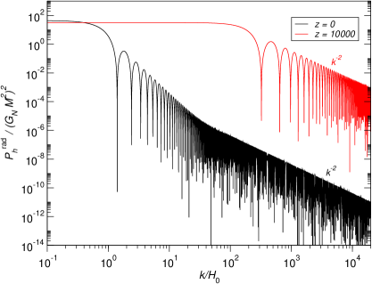
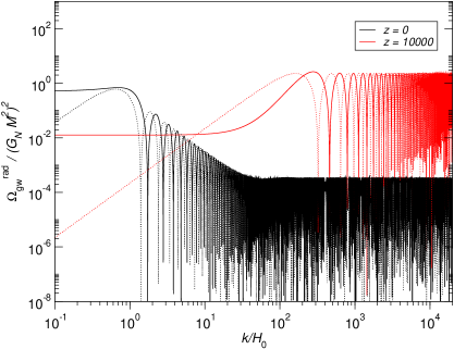
Figure 1: The normalised strain power spectrum $\mathcal{P}_{h}^{\mathrm{rad}}/(G_{\mathrm{{\scriptscriptstyle{N}}}}M^{2})^{2}$ (left panel) and energy density parameter $\Omega_{\mathrm{gw}}^{\mathrm{rad}}/(G_{\mathrm{{\scriptscriptstyle{N}}}}M^{2})^{2}$ (right panel) coming from extinct sources in the radiation era, measured either at $z=10^{4}$ (red curve) or in the matter era, today, at $z=0$ (black curve). For illustration purposes, the Fourier transform of the source correlator is set to $\hat{C}_{\mathrm{ini}}^{\mathrm{rad}}(1,1)=1$. Notice the change of slope for $k>1/\eta_{\mathrm{eq}}$ for $z=0$. The dotted curves on the right panel shows $k^{2}/(12\mathcal{H}_{0})^{2}\mathcal{P}_{h}^{\mathrm{rad}}$ which deviates from $\Omega_{\mathrm{gw}}^{\mathrm{rad}}$ on large scales and oscillates in phase opposition at small scales.

In figure 1 we have represented the normalised strain power spectrum (left panel) and the energy density parameter (right panel), at equal times, as a function of $k/\mathcal{H}_{0}$. Two measurement redshifts have been represented, one in the radiation era at $z=10^{4}$, and one today at $z=0$. For the latter, we see that the spectrum dependence with respect to the wavenumbers changes at scales matching equality $k=1/\eta_{\mathrm{eq}}$. In the right panel of this figure, we have compared the usual approximation $k^{2}/(12\mathcal{H}_{0}^{2})\mathcal{P}_{h}^{\mathrm{rad}}$, plotted as dotted curves, to the actual value of $\Omega_{\mathrm{gw}}^{\mathrm{rad}}$. The envelope of both matches well inside the Hubble radius, but they do oscillate in phase opposition at large wavenumbers. In fact, a better approximation can be obtained from equation (3.6), (3.16) and (3.20), assuming the integral to have all the same typical amplitude, one has

$$\Omega_{\mathrm{gw}}^{\mathrm{rad}}(\eta_{1},\eta_{2},k\gg\mathcal{H})\simeq\dfrac{k^{2}}{12\mathcal{H}(\eta_{1})\mathcal{H}(\eta_{2})}\dfrac{\partial^{2}\mathcal{P}_{h}^{\mathrm{rad}}}{\partial x_{1}\partial x_{2}}\,.$$ (3.53)

Notice that the envelope of the oscillations plotted in figure 1 matches the typical behaviour derived in Refs. [30, 31], within the level of their approximation. On the very large scales, both $\mathcal{P}_{h}^{\mathrm{rad}}$ and $\Omega_{\mathrm{gw}}^{\mathrm{rad}}$ are scale invariant for extinct sources and the approximation of equation (3.53) is also violated. Let us mention that, as discussed in more details in section 3.6, requiring the source to be extinct for $k\to 0$ is very contriving as the lifetime, or spatial extension, of the sources should be irrealistically small.

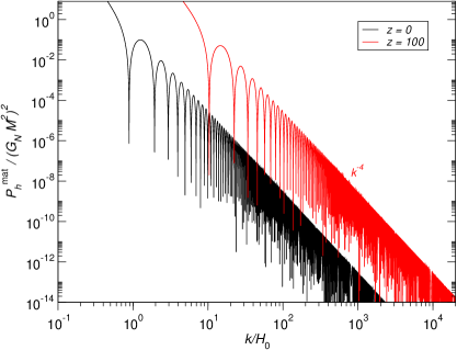
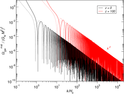
Figure 2: The normalized strain power spectrum $\mathcal{P}_{h}^{\mathrm{mat}}/(G_{\mathrm{{\scriptscriptstyle{N}}}}M^{2})^{2}$ (left panel) and energy density parameter $\Omega_{\mathrm{gw}}^{\mathrm{mat}}/(G_{\mathrm{{\scriptscriptstyle{N}}}}M^{2})^{2}$ (right panel) coming from extinct sources in the matter era, measured either at $z=10^{2}$ (red curve) or today at $z=0$ (black curve). For illustration purposes, the Fourier transform of the source correlators is set to $\hat{C}_{\mathrm{eq}}^{\mathrm{mat}}(1,1)=1$, $\hat{D}_{\mathrm{eq}}^{\mathrm{mat}}(1,1)=0$ and $\hat{E}_{\mathrm{eq}}^{\mathrm{mat}}(1,1)=0$, which is the dominant term at wavenumbers $1/\eta_{0}\ll k\ll 1/\eta_{\mathrm{eq}}$. The dotted curves on the right panel shows $k^{2}/(12\mathcal{H}_{0})^{2}\mathcal{P}_{h}^{\mathrm{mat}}$ which oscillates in phase opposition of $\Omega_{\mathrm{gw}}^{\mathrm{mat}}$ at small scales. The envelope of both curves decays as expected in $1/k^{2}$.

The derivation of the equal-time contribution coming from the matter era extinct sources can be performed in a similar way, paying attention that the functions $\hat{a}(x,k)$ are different. In the matter era, one has

$$\hat{a}_{i}(x,k)=\dfrac{(x+x_{\mathrm{eq}})^{2}}{\left[k\left(\eta_{i}+\eta_{\mathrm{eq}}\right)\right]^{2}}\,,$$ (3.54)

and

$$\hat{\mathcal{C}}_{k}^{\mathrm{mat}}(1,1)=\dfrac{1}{k^{4}(\eta_{1}+\eta_{\mathrm{eq}})^{2}(\eta_{2}+\eta_{\mathrm{eq}})^{2}}\hat{C}_{\mathrm{eq}}^{\mathrm{mat}}(1,1),$$ (3.55)

with $\hat{C}_{\mathrm{eq}}^{\mathrm{mat}}(\gamma,\gamma^{\prime})$ the Fourier transform of

$$C_{\mathrm{eq}}^{\mathrm{mat}}(y,y^{\prime})=\dfrac{\left(2x_{\mathrm{eq}}+|y|\right)^{2}\left(2x_{\mathrm{eq}}+|y^{\prime}|\right)^{2}}{\sqrt{x_{\mathrm{eq}}+|y|}\,\sqrt{x_{\mathrm{eq}}+|y^{\prime}|}}\mathcal{U}^{\mathrm{mat}}(x_{\mathrm{eq}}+|y|,x_{\mathrm{eq}}+|y^{\prime}|).$$ (3.56)

The other correlators are $D_{\mathrm{eq}}^{\mathrm{mat}}=C_{\mathrm{eq}}^{\mathrm{mat}}/(2x_{\mathrm{eq}}+|y|)$ and $E_{\mathrm{eq}}^{\mathrm{mat}}=C_{\mathrm{eq}}^{\mathrm{mat}}/[(2x_{\mathrm{eq}}+|y|)(2x_{\mathrm{eq}}+|y^{\prime}|)]$ and one has to perform three Fourier transforms to determine the matter era power spectrum. However, $D_{\mathrm{eq}}^{\mathrm{mat}}$ and $E_{\mathrm{eq}}^{\mathrm{mat}}$ are smaller than $C_{\mathrm{eq}}^{\mathrm{mat}}(y,y^{\prime})$ when $2x_{\mathrm{eq}}+|y|>1$ but could dominate otherwise. The index “eq” here is a reminder that there is an implicit dependence in $k$ through the parameter $x_{\mathrm{eq}}=k\eta_{\mathrm{eq}}$. For $k\ll 1/\eta_{\mathrm{eq}}$, this dependence is negligible and $\hat{C}_{\mathrm{eq}}^{\mathrm{mat}}(1,1)$ should be roughly constant. In figure 2, we have represented the resulting $\mathcal{P}_{h}^{\mathrm{mat}}$ as a function of $k/\mathcal{H}_{0}$ by setting $\hat{C}_{\mathrm{eq}}^{\mathrm{mat}}(1,1)=1$ with $\hat{D}_{\mathrm{eq}}^{\mathrm{mat}}(1,1)=0$ and $\hat{E}_{\mathrm{eq}}^{\mathrm{mat}}(1,1)=0$. These plots should be typical of matter era extinct sources but only in the intermediate range $1/\eta_{0}\ll k\ll 1/\eta_{\mathrm{eq}}$. Indeed, as soon as $k>1/\eta_{\mathrm{eq}}$, one does not expect $\hat{C}_{\mathrm{eq}}^{\mathrm{mat}}(1,1)$ to be constant any more and only a precise knowledge of the function $\mathcal{U}^{\mathrm{mat}}(x,x^{\prime})$ would allow us to determine how it varies with $k$. For instance, if $\mathcal{U}^{\mathrm{mat}}(x,x^{\prime})$ rapidly decays for $x>x_{\mathrm{eq}}$ (and $x^{\prime}>x_{\mathrm{eq}}$), faster than $(xx^{\prime})^{-3/2}$, equation (3.56) shows that $\hat{C}_{\mathrm{eq}}^{\mathrm{mat}}(1,1)\to 0$ and the spectra represented in figure 2 could decay faster than the represented $\mathcal{P}_{h}^{\mathrm{mat}}\propto k^{-4}$ at $k\gg 1/\eta_{\mathrm{eq}}$. Nonetheless, in the regime represented, the small scale approximation

$$\Omega_{\mathrm{gw}}^{\mathrm{mat}}(\eta_{1},\eta_{2},k\gg\mathcal{H})\simeq\dfrac{k^{2}}{12\mathcal{H}(\eta_{1})\mathcal{H}(\eta_{2})}\dfrac{\partial^{2}\mathcal{P}_{h}^{\mathrm{mat}}}{\partial x_{1}\partial x_{2}}\,,$$ (3.57)

also holds. On the large scales, for $k<1$, one cannot neglect any more the other Fourier transforms $\hat{D}_{\mathrm{eq}}^{\mathrm{mat}}(1,1)$ and $\hat{E}_{\mathrm{eq}}^{\mathrm{mat}}(1,1)$. Moreover, as already mentioned, the assumption of extinct sources on the largest scales is very contriving.

3.6 Large scales and constant sources

The waveforms obtained in equations (3.40), (3.41), (3.45), (3.46), (3.49) and (B.4) are exact provided the function $\mathcal{C}_{k}(y,y^{\prime})$ is compactly supported in addition to be square integrable. This ensures that its Fourier transform is holomorphic (see appendix A). From the definition of $\mathcal{C}_{k}(y,y^{\prime})$ given in equation (3.26), this will be the case if $\mathcal{U}(x,x^{\prime})$ has compact support, i.e., there should exist a domain in the plane $(x,x^{\prime})$ outside of which the correlator is vanishing. As an example, let us assume that we require $\mathcal{U}_{r}(x>x_{0},x^{\prime}>x_{0})=0$ with $x_{0}<x_{1}$ and $x_{0}<x_{2}$. From the definition of the scaling correlator in equation (3.1), this implies that the anisotropic stress $\varPi_{r}(\xi,k)$ can only be non-vanishing in a domain of the plane $(\xi,k)$ verifying $\xi<x_{0}/k$, which is very restrictive if $x_{0}$ is small. Conversely, if the anisotropic stress $\varPi(\xi,k)$ vanishes for $\xi>\xi_{0}$, $\mathcal{U}(x,x^{\prime})$ will only be compactly supported if there exists a wavenumber $k_{0}$ above which $\varPi(\xi,k>k_{0})=0$ and one gets $x_{0}=k_{0}\xi_{0}$. Here again, we see that small values of $x_{0}$ would be very contriving, either on the time during which the source can be active, or on its spatial structure which should not excite high wavenumbers. It may be possible to relax somehow these constraints by requiring the correlators to belong the Schwartz space but the physical requirements for smoothness and time-limited sources will certainly remain.

Even though the formulas obtained for extinct sources are not approximation, we thus expect the regime for which they have been derived to break down at large scale for any realistic anisotropic stresses. This is illustrated by the infrared divergence of $\mathcal{P}_{h}^{\mathrm{mat}}$ in figure 2. Interestingly, for scaling sources such as cosmic defects, the correlators $\mathcal{U}(x,x^{\prime})$ are usually trivial at small $x$ and $x^{\prime}$ as they become constant.

Let us assume that $\mathcal{U}(x,x^{\prime})=\mathcal{U}_{0}$, a constant, for all $x\leq x_{1}$ and $x^{\prime}\leq x_{2}$. This condition implies that it is not compactly supported within the domain of integration and the expression obtained from extinct sources are no longer applicable. However, the integral $I_{\mu}$ can again be derived exactly. In the radiation era, using equations (3.7), (3.10) and (3.50), one finds

$$I_{\mu}^{\mathrm{rad}}(x_{1},x_{2},k) =\dfrac{\mathcal{U}_{0}^{\mathrm{rad}}}{k^{2}\eta_{1}\eta_{2}}\bigg{\{}\sqrt{x_{1}}-\cos(x_{1}-x_{\mathrm{ini}})\sqrt{x_{\mathrm{ini}}}-\sin(x_{1})\left[\operatorname{\bar{S}_{2}}(x_{1})-\operatorname{\bar{S}_{2}}(x_{\mathrm{ini}})\right]$$ (3.58)

$$-\cos(x_{1})\left[\operatorname{\bar{C}_{2}}(x_{1})-\operatorname{\bar{C}_{2}}(x_{\mathrm{ini}})\right]\bigg{\}}\times\bigg{\{}\sqrt{x_{2}}-\cos(x_{2}-x_{\mathrm{ini}})\sqrt{x_{\mathrm{ini}}}$$

$$-\sin(x_{2})\left[\operatorname{\bar{S}_{2}}(x_{2})-\operatorname{\bar{S}_{2}}(x_{\mathrm{ini}})\right]-\cos(x_{2})\left[\operatorname{\bar{C}_{2}}(x_{2})-\operatorname{\bar{C}_{2}}(x_{\mathrm{ini}})\right]\bigg{\}},$$

where we have introduced the unnormalised Fresnel integrals [35]

$$\operatorname{\bar{C}_{2}}(x)=\dfrac{1}{2}\int_{0}^{x}\dfrac{\cos(t)}{\sqrt{t}}\mathrm{d}t,\qquad\operatorname{\bar{S}_{2}}(x)=\dfrac{1}{2}\int_{0}^{x}\dfrac{\sin(t)}{\sqrt{t}}\mathrm{d}t.$$ (3.59)

In the large scale limit $x_{1}\to 0$ and $x_{2}\to 0$, still assuming $x_{\mathrm{ini}}\ll x_{1}$ and $x_{\mathrm{ini}}\ll x_{2}$, one gets

$$I_{\mu}^{\mathrm{rad}}(x_{1},x_{2},k)\simeq\dfrac{16}{225}\mathcal{U}_{0}^{\mathrm{rad}}\left(x_{1}x_{2}\right)^{3/2},$$ (3.60)

which shows that the strain power spectrum varies as $\mathcal{P}_{h}^{\mathrm{rad}}\propto k^{3}$, at large scales. The $I_{\mu}^{\mathrm{mat}}$ integral stemming from a constant correlator $\mathcal{U}(x,x^{\prime})=\mathcal{U}_{0}^{\mathrm{mat}}$ in the matter era can also be analytically derived. From equations (3.4), (3.5) and (3.54), one obtains

$$I_{\mu}^{\mathrm{mat}}(x_{1},x_{2},k)=\dfrac{\mathcal{U}_{0}^{\mathrm{mat}}}{4k^{4}(\eta_{1}+\eta_{\mathrm{eq}})^{2}(\eta_{2}+\eta_{\mathrm{eq}})^{2}(x_{1}+x_{\mathrm{eq}})(x_{2}+x_{\mathrm{eq}})}$$

$$\times\bigg{\{}\sqrt{x_{1}}\left[5+2(x_{1}+x_{\mathrm{eq}})(x_{1}+2x_{\mathrm{eq}})\right]$$

$$-\sqrt{x_{\mathrm{eq}}}\left[5+6x_{\mathrm{eq}}(x_{1}+x_{\mathrm{eq}})\right]\cos(x_{1}-x_{\mathrm{eq}})+\sqrt{x_{\mathrm{eq}}}\left(x_{\mathrm{eq}}-5x_{1}\right)\sin(x_{1}-x_{\mathrm{eq}})$$

$$+\left[\left(5+8x_{\mathrm{eq}}x_{1}+4x_{\mathrm{eq}}^{2}\right)\cos(x_{1})+\left(5x_{1}-3x_{\mathrm{eq}}-4x_{1}x_{\mathrm{eq}}^{2}-4x_{\mathrm{eq}}^{3}\right)\sin(x_{1})\right]\left[\operatorname{\bar{C}_{2}}(x_{\mathrm{eq}})-\operatorname{\bar{C}_{2}}(x_{1})\right]$$

$$+\left[\left(5+8x_{\mathrm{eq}}x_{1}+4x_{\mathrm{eq}}^{2}\right)\sin(x_{1})-\left(5x_{1}-3x_{\mathrm{eq}}-4x_{1}x_{\mathrm{eq}}^{2}-4x_{\mathrm{eq}}^{3}\right)\cos(x_{1})\right]\left[\operatorname{\bar{S}_{2}}(x_{\mathrm{eq}})-\operatorname{\bar{S}_{2}}(x_{1})\right]\bigg{\}}$$

$$\times\bigg{\{}\sqrt{x_{2}}\left[5+2(x_{2}+x_{\mathrm{eq}})(x_{2}+2x_{\mathrm{eq}})\right]$$

$$-\sqrt{x_{\mathrm{eq}}}\left[5+6x_{\mathrm{eq}}(x_{2}+x_{\mathrm{eq}})\right]\cos(x_{2}-x_{\mathrm{eq}})+\sqrt{x_{\mathrm{eq}}}\left(x_{\mathrm{eq}}-5x_{2}\right)\sin(x_{2}-x_{\mathrm{eq}})$$

$$+\left[\left(5+8x_{\mathrm{eq}}x_{2}+4x_{\mathrm{eq}}^{2}\right)\cos(x_{2})+\left(5x_{2}-3x_{\mathrm{eq}}-4x_{2}x_{\mathrm{eq}}^{2}-4x_{\mathrm{eq}}^{3}\right)\sin(x_{2})\right]\left[\operatorname{\bar{C}_{2}}(x_{\mathrm{eq}})-\operatorname{\bar{C}_{2}}(x_{2})\right]$$

$$+\left[\left(5+8x_{\mathrm{eq}}x_{2}+4x_{\mathrm{eq}}^{2}\right)\sin(x_{2})-\left(5x_{2}-3x_{\mathrm{eq}}-4x_{2}x_{\mathrm{eq}}^{2}-4x_{\mathrm{eq}}^{3}\right)\cos(x_{2})\right]\left[\operatorname{\bar{S}_{2}}(x_{\mathrm{eq}})-\operatorname{\bar{S}_{2}}(x_{2})\right]\bigg{\}}.$$ (3.61)

In the large scale limits $x_{1}\to 0$ and $x_{2}\to 0$ with $x_{\mathrm{eq}}\ll x_{1}$ and $x_{\mathrm{eq}}\ll x_{2}$, it simplifies to

$$I_{\mu}^{\mathrm{mat}}(x_{1},x_{2},k)\simeq\dfrac{16}{729}\mathcal{U}_{0}^{\mathrm{mat}}\left(x_{1}x_{2}\right)^{3/2},$$ (3.62)

which again implies that $\mathcal{P}_{h}^{\mathrm{mat}}\propto k^{3}$ on the largest scales.

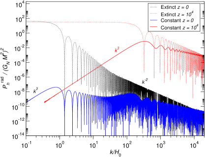
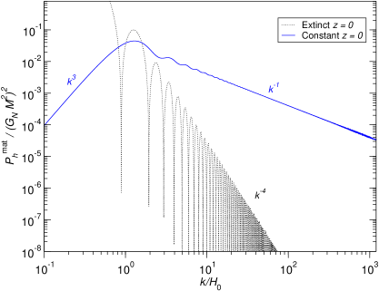
Figure 3: The normalised strain power spectrum $\mathcal{P}_{h}^{\mathrm{rad}}/(G_{\mathrm{{\scriptscriptstyle{N}}}}M^{2})^{2}$ (left panel) and $\mathcal{P}_{h}^{\mathrm{mat}}/(G_{\mathrm{{\scriptscriptstyle{N}}}}M^{2})^{2}$ (right panel) generated by constant sources, i.e., having a strictly constant correlator $\mathcal{U}(x,x^{\prime})=\mathcal{U}_{0}$ over the whole integration domain. The power spectrum generated during the radiation era is represented at $z=10^{4}$, but also propagated down to the matter era at $z=0$. The dotted curves are the strain spectra associated with extinct sources (see figures 1 and 2). For illustration purposes, we have arbitrarily set $\mathcal{U}_{0}^{\mathrm{mat}}=\mathcal{U}_{0}^{\mathrm{rad}}=10^{-3}$. We expect realistic, but non-singular, scaling sources to be “constant” at small wavenumbers (as depicted in this figure) while behaving as “extinct” above some given wavenumber.

From equations (3.58) and (3.61), one could derive exact analytical formulas for the waveforms of all the observable quantities, $\mathcal{P}_{h}^{\mathrm{rad}}$, $\mathcal{P}_{h}^{\mathrm{mat}}$, $\Omega_{\mathrm{gw}}^{\mathrm{mat}}$ and $\Omega_{\mathrm{gw}}^{\mathrm{rad}}$. Obviously, these expressions would only be valid in the $(x_{1},x_{2})$ domains for which $\mathcal{U}(x,x^{\prime})$ remains strictly constant. We do not report these calculations here, but, as an illustration, we have plotted in figure 3, the shape of the radiation and matter era strain power spectrum stemming from equations (3.58) and (3.61), respectively. For comparison, we have reported the spectra associated with the extinct sources of figures 1 and 2. Firstly, one can notice that, for constant correlators, the oscillations are not maximal and only induce small modulations with respect to the overall amplitude. This can be understood from equations (3.58) and (3.61). Oscillatory terms have a prefactor scaling as a positive power of $x_{\mathrm{eq}}$ in the matter era (and $x_{\mathrm{ini}}$ in the radiation era), which is always smaller than $x_{1}$ and $x_{2}$. Moreover, all the Fresnel integrals appear as differences, as in $\operatorname{\bar{C}_{2}}(x_{\mathrm{eq}})-\operatorname{\bar{C}_{2}}(x_{1})$, and they vanish asymptotically. As such, they can never drive the overall shape of the spectra. This contrasts with the spectra associated with extinct scaling sources. Because we do not expect $\mathcal{U}(x,x^{\prime})$ to remain constant for $x_{1}$ and $x_{2}$ large, the strain power spectra associated with realistic scaling sources should be matching the constant correlator behaviour at small wavenumbers, up to some wavenumber at which it turns into an extinct sources spectra. Let us notice that, focusing only on the spectra envelope, and omitting the differences between $\Omega_{\mathrm{gw}}$ and $\mathcal{P}_{h}$, such a behaviour is the one discussed in Refs. [30, 31]. As such, it could be considered as the standard lore for scaling sources and we have now added its complete time and wavenumber dependence.

However, as we discuss in the next section, it is possible for certain scaling sources to produce a singular Fourier transform $\hat{\mathcal{C}}(\gamma,\gamma^{\prime})$ from a non-square integrable function $\mathcal{C}(y,y^{\prime})$ while having a regular correlator $\mathcal{U}(x,x^{\prime})$.

3.7 Small scales and singular sources

In view of the previous discussion, it is instructive to discuss scaling sources that could possibly break the assumption of being “extinct” on all length scales. A sufficient condition for this to happen is that the Fourier transform $\hat{\mathcal{C}}(\gamma,\gamma^{\prime})$ should be singular for some value of $\gamma$ and $\gamma^{\prime}$.

As an example, let us consider a perfectly coherent correlator that behaves at large $x$ and $x^{\prime}$ as

$$\mathcal{U}(x\gg 1,x^{\prime}\gg 1)=\dfrac{\mathcal{U}_{\infty}}{\sqrt{xx^{\prime}}}\,,$$ (3.63)

where $\mathcal{U}_{\infty}$ is a constant. For $x=x^{\prime}$, the correlator slowly decays with the wavenumber as $1/k$ and such a behaviour is reminiscent with the small scales behaviour of the two-point correlation functions associated with a random distribution of line-like objects such as long cosmic strings [48, 47, 49, 50].

In the radiation era, at large enough $y$ and $y^{\prime}$, from equations (3.52), one gets

$$C_{\mathrm{ini}}^{\mathrm{rad}}(y,y^{\prime})=\mathcal{U}_{\infty}^{\mathrm{rad}}\implies\hat{C}_{\mathrm{ini}}^{\mathrm{rad}}(\gamma,\gamma^{\prime})=(2\pi)^{2}\mathcal{U}_{\infty}^{\mathrm{rad}}\delta(\gamma)\delta(\gamma^{\prime}),$$ (3.64)

and the Fourier transform $\hat{\mathcal{C}}_{k}^{\mathrm{rad}}$ is a distribution, singular at the origin of the plane $(\gamma,\gamma^{\prime})$. It reads

$$\hat{\mathcal{C}}_{k}^{\mathrm{rad}}(\gamma,\gamma^{\prime})=(2\pi)^{2}\dfrac{\mathcal{U}_{\infty}^{\mathrm{rad}}}{k^{2}\eta_{1}\eta_{2}}\,\delta(\gamma)\delta(\gamma^{\prime}).$$ (3.65)

Plugging this expression into the integrals $I_{\mathrm{cc}}$, $I_{\mathrm{cs}}$, $I_{\mathrm{sc}}$ and $I_{\mathrm{ss}}$ given by equations (3.29), (3.33), (3.36) and (3.37) gives a completely different result than the extinct case. In particular, $I_{\mathrm{ss}}$, $I_{\mathrm{cs}}$ and $I_{\mathrm{sc}}$ are now non-vanishing and read

$$I_{\mathrm{cc}}(y_{1},y_{2},k) =\dfrac{\mathcal{U}_{\infty}^{\mathrm{rad}}}{k^{2}\eta_{1}\eta_{2}}\sin(y_{1})\sin(y_{2}),\qquad I_{\mathrm{ss}}(y_{1},y_{2},k) =\dfrac{4\mathcal{U}_{\infty}^{\mathrm{rad}}}{k^{2}\eta_{1}\eta_{2}}\sin^{2}\left(\dfrac{y_{1}}{2}\right)\sin^{2}\left(\dfrac{y_{2}}{2}\right),$$ (3.66)

$$I_{\mathrm{cs}}(y_{1},y_{2},k) =\dfrac{2\mathcal{U}_{\infty}^{\mathrm{rad}}}{k^{2}\eta_{1}\eta_{2}}\sin(y_{1})\sin^{2}\left(\dfrac{y_{2}}{2}\right),\qquad I_{\mathrm{sc}}(y_{1},y_{2},k) =\dfrac{2\mathcal{U}_{\infty}^{\mathrm{rad}}}{k^{2}\eta_{1}\eta_{2}}\sin^{2}\left(\dfrac{y_{1}}{2}\right)\sin(y_{2}).$$

From equation (3.24), one obtains

$$I_{\mu}^{\mathrm{rad}}(x_{1},x_{2},k)=\dfrac{4\mathcal{U}_{\infty}^{\mathrm{rad}}}{k^{2}\eta_{1}\eta_{2}}\sin^{2}\left(\dfrac{x_{1}-x_{\mathrm{ini}}}{2}\right)\sin^{2}\left(\dfrac{x_{2}-x_{\mathrm{ini}}}{2}\right),$$ (3.67)

from which the strain power spectrum reads

$$\mathcal{P}_{h}^{\mathrm{rad}}(\eta_{1}<\eta_{\mathrm{eq}},\eta_{2}<\eta_{\mathrm{eq}},k) =128\left(G_{\mathrm{{\scriptscriptstyle{N}}}}M^{2}\right)^{2}\dfrac{\mathcal{U}_{\infty}^{\mathrm{rad}}}{k^{2}\eta_{1}\eta_{2}}\bigg{\{}1-\cos(x_{1}-x_{\mathrm{ini}})-\cos(x_{2}-x_{\mathrm{ini}})$$ (3.68)

$$+\dfrac{1}{2}\cos(x_{1}-x_{2})+\dfrac{1}{2}\cos(x_{1}+x_{2}-2x_{\mathrm{ini}})\bigg{\}}.$$

This expression has to be compared to the one for extinct sources in equation (3.40), together with equation (3.51) (see also figure 1). The amplitude in front of each oscillatory function is different and so are their associated waveform. For instance, focusing on the equal-time spectra with $x_{1}=x_{2}=x_{0}$, we see that the strain spectrum for extinct sources varies as $[\sin(x_{0}-x_{\mathrm{ini}})]^{2}/k^{2}$ whereas the singular one goes as $\{\sin[(x_{0}-x_{\mathrm{ini}})/2]\}^{4}/k^{2}$. Some oscillations have disappeared as if interferences were appearing. Notice that focusing only on their envelope, both spectra decay as $1/k^{2}$ and would be undistinguishable without looking at their fine structure. Deriving equation (3.67) with respect to $x_{1}$ and $x_{2}$ gives the other integrals

$$I_{\mu^{\prime}}^{\mathrm{rad}}(x_{1},x_{2},k)=\dfrac{\mathcal{U}_{\infty}^{\mathrm{rad}}}{k^{2}\eta_{1}\eta_{2}}\sin(x_{1}-x_{\mathrm{ini}})\sin(x_{1}-x_{\mathrm{ini}}),$$ (3.69)

and

$$I_{\kappa}^{\mathrm{rad}}(x_{1},x_{2},k)=\dfrac{2\mathcal{U}_{\infty}^{\mathrm{rad}}}{k^{2}\eta_{1}\eta_{2}}\sin(x_{1}-x_{\mathrm{ini}})\sin^{2}\left(\dfrac{x_{2}-x_{\mathrm{ini}}}{2}\right).$$ (3.70)

These integrals evaluated at $x_{1}=x_{2}=x_{\mathrm{eq}}$ allow us to derive the radiation strain spectrum for the singular source propagated in the matter era by using equations (3.8) and (3.18). They inherit the $1/k^{2}$ behaviour in their envelope while the waveform measured at any $\eta_{i}>\eta_{\mathrm{eq}}$ is driven by the $A_{i}$ and $B_{i}$ functions. However, there is also an additional modulation which is induced by the functions $I_{\mu}^{\mathrm{rad}}(x_{\mathrm{eq}},x_{\mathrm{eq}},k)$, $I_{\mu^{\prime}}^{\mathrm{rad}}(x_{\mathrm{eq}},x_{\mathrm{eq}},k)$ and $I_{\kappa}^{\mathrm{rad}}(x_{\mathrm{eq}},x_{\mathrm{eq}},k)$. This modulation is visible, and compared to the extinct spectrum, in the right panel of figure 4. Here as well, only the presence of these interferences would signal a singular source at large wavenumbers. Let us also notice that these modulations involve terms in $x_{\mathrm{eq}}-x_{\mathrm{ini}}\simeq k\eta_{\mathrm{eq}}$ for $\eta_{\mathrm{ini}}\ll\eta_{\mathrm{eq}}$. Therefore, in real space, the typical length associated with these interferences is about the Hubble radius at equality, i.e., of the order of $100\,\mathrm{Mpc}$. There are also differences at smaller wavenumbers but, as mentioned before, the correlator should behave as constant on these scales and equation (3.63) may not be applicable (see section 3.6).

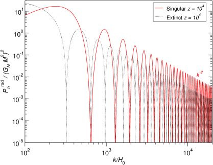
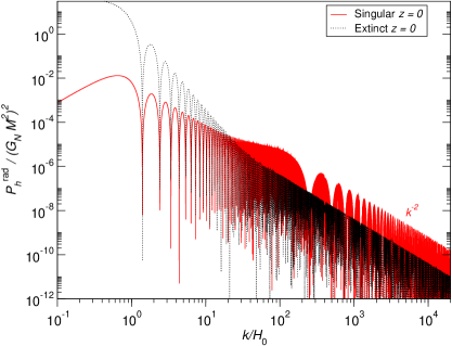
Figure 4: The normalised strain power spectrum $\mathcal{P}_{h}^{\mathrm{rad}}/(G_{\mathrm{{\scriptscriptstyle{N}}}}M^{2})^{2}$ generated in the radiation era by a singular source having a correlator $\mathcal{U}(x,x^{\prime})=\mathcal{U}_{\infty}/\sqrt{xx^{\prime}}$. The left panel shows the strain spectrum generated and evaluated in the radiation era ($z=10^{4}$) whereas the right panel shows the same spectrum propagated and evaluated in the matter era ($z=0$). The strain spectrum from extinct sources is represented as dotted curves. Both have an envelope decreasing as $k^{-2}$ at large wavenumbers but exhibit completely different oscillatory patterns, as if the singular sources were generating interferences. For illustration purposes, we have set $\mathcal{U}_{\infty}=1$.

We can also derive the energy density spectrum within the radiation era, as given by equation (3.16). Since all integrals are of the same typical amplitude, at small scales, one has

$$\Omega_{\mathrm{gw}}^{\mathrm{rad}}(\eta_{1}<\eta_{\mathrm{eq}},\eta_{2}<\eta_{\mathrm{eq}},k\gg\mathcal{H})\simeq\dfrac{32}{3}\left(G_{\mathrm{{\scriptscriptstyle{N}}}}M^{2}\right)^{2}\dfrac{\mathcal{U}_{\infty}^{\mathrm{rad}}}{\eta_{1}\mathcal{H}_{1}\eta_{2}\mathcal{H}_{2}}\sin(x_{1}-x_{\mathrm{ini}})\sin(x_{2}-x_{\mathrm{ini}}),$$ (3.71)

which is, as expected, proportional to the double derivative of $\partial^{2}\mathcal{P}_{h}^{\mathrm{rad}}/\partial x_{1}\partial x_{2}$. Interestingly, the “interferences” are no longer present for $\Omega_{\mathrm{gw}}^{\mathrm{rad}}$ and it behaves almost exactly as the one associated with extinct sources, see equations (3.39) and (3.41). It oscillates with a product of sine functions instead of a product of cosine functions and both end-up only differing by a phase shift of $\pi/2$ at large wavenumbers.

The singular source of equation (3.63) induces more pronounced effects in the matter era. From equation (3.56) one gets

$$C_{\mathrm{eq}}^{\mathrm{mat}}(y,y^{\prime})=\dfrac{(2x_{\mathrm{eq}}+|y|)^{2}(2x_{\mathrm{eq}}+|y^{\prime}|)^{2}}{(x_{\mathrm{eq}}+|y|)(x_{\mathrm{eq}}+|y^{\prime}|)}\mathcal{U}_{\infty}^{\mathrm{mat}},$$ (3.72)

which is a growing function of $(y,y^{\prime})$. It can be separated into three terms according to their behaviour at large $(y,y^{\prime})$

$$C_{\mathrm{eq}}^{\mathrm{mat}}(y,y^{\prime}) =\mathcal{U}_{\infty}^{\mathrm{mat}}(x_{\mathrm{eq}}+|y|)(x_{\mathrm{eq}}+|y^{\prime}|)$$ (3.73)

$$+\mathcal{U}_{\infty}^{\mathrm{mat}}x_{\mathrm{eq}}\left[\dfrac{(3x_{\mathrm{eq}}+2|y|)(x_{\mathrm{eq}}+|y^{\prime}|)}{x_{\mathrm{eq}}+|y|}+\dfrac{(3x_{\mathrm{eq}}+2|y^{\prime}|)(x_{\mathrm{eq}}+|y|)}{x_{\mathrm{eq}}+|y^{\prime}|}\right]$$

$$+\mathcal{U}_{\infty}^{\mathrm{mat}}x_{\mathrm{eq}}^{2}\dfrac{(3x_{\mathrm{eq}}+2|y|)(3x_{\mathrm{eq}}+2|y^{\prime}|)}{(x_{\mathrm{eq}}+|y|)(x_{\mathrm{eq}}+|y^{\prime}|)}\,.$$

The first term is the one that dominates asymptotically and, to simplify the discussion, we focus only on this one. Moreover, doing so is consistent with neglecting the other functions $D_{\mathrm{eq}}^{\mathrm{mat}}(y,y^{\prime})$ and $E_{\mathrm{eq}}^{\mathrm{mat}}(y,y^{\prime})$ at large wavenumbers. We have for the Fourier transform

$$\hat{\mathcal{C}}_{k}^{\mathrm{mat}}(\gamma,\gamma^{\prime})\simeq\dfrac{\mathcal{U}_{\infty}^{\mathrm{mat}}}{k^{4}(\eta_{1}+\eta_{\mathrm{eq}})^{2}(\eta_{2}+\eta_{\mathrm{eq}})^{2}}\left[2\pi x_{\mathrm{eq}}\delta(\gamma)-\dfrac{2}{\gamma^{2}}\right]\left[2\pi x_{\mathrm{eq}}\delta(\gamma^{\prime})-\dfrac{2}{\gamma^{\prime 2}}\right].$$ (3.74)

Clearly not holomorphic as it contains Dirac distributions as well as power law terms in $1/\gamma^{2}$ and $1/\gamma^{\prime 2}$, all singular at the origin $\gamma=\gamma^{\prime}=0$. These terms explicitly break the extinct sources calculations. Ignoring the other functions $\hat{\mathcal{D}}_{\mathrm{eq}}^{\mathrm{mat}}$ and $\hat{\mathcal{E}}_{\mathrm{eq}}^{\mathrm{mat}}$, and considering only the asymptotic form of the matter era Green’s functions, one obtains, for the four basic integrals, the following approximations

$$I_{\mathrm{cc}}(y_{1},y_{2},k\gg\mathcal{H}) \simeq\dfrac{\mathcal{U}_{\infty}^{\mathrm{mat}}}{k^{4}(\eta_{1}+\eta_{\mathrm{eq}})^{2}(\eta_{2}+\eta_{\mathrm{eq}})^{2}}\left[(x_{\mathrm{eq}}+y_{1})\sin(y_{1})+\cos(y_{1})-1\right]$$ (3.75)

$$\times\left[(x_{\mathrm{eq}}+y_{2})\sin(y_{2})+\cos(y_{2})-1\right],$$

$$I_{\mathrm{ss}}(y_{1},y_{2},k\gg\mathcal{H}) \simeq\dfrac{\mathcal{U}_{\infty}^{\mathrm{mat}}}{k^{4}(\eta_{1}+\eta_{\mathrm{eq}})^{2}(\eta_{2}+\eta_{\mathrm{eq}})^{2}}\left\{x_{\mathrm{eq}}[1-\cos(y_{1})]-y_{1}\cos(y_{1})+\sin(y_{1})\right\}$$

$$\times\left\{x_{\mathrm{eq}}[1-\cos(y_{2})]-y_{2}\cos(y_{2})+\sin(y_{2})\right\},$$

and

$$I_{\mathrm{cs}}(y_{1},y_{2},k\gg\mathcal{H}) =\dfrac{\mathcal{U}_{\infty}^{\mathrm{mat}}}{k^{4}(\eta_{1}+\eta_{\mathrm{eq}})^{2}(\eta_{2}+\eta_{\mathrm{eq}})^{2}}\left[(x_{\mathrm{eq}}+y_{1})\sin(y_{1})+\cos(y_{1})-1\right]$$ (3.76)

$$\times\left\{x_{\mathrm{eq}}[1-\cos(y_{2})]-y_{2}\cos(y_{2})+\sin(y_{2})\right\},$$

with $I_{\mathrm{sc}}(y_{1},y_{2},k)=I_{\mathrm{cs}}(y_{2},y_{1},k)$. Finally, one gets

$$I_{\mu}^{\mathrm{mat}}(x_{1},x_{2},k\gg\mathcal{H}) \simeq\dfrac{\mathcal{U}_{\infty}^{\mathrm{mat}}}{k^{4}(\eta_{1}+\eta_{\mathrm{eq}})^{2}(\eta_{2}+\eta_{\mathrm{eq}})^{2}}\left[x_{1}-x_{\mathrm{eq}}\cos(x_{1}-x_{\mathrm{eq}})-\sin(x_{1}-x_{\mathrm{eq}})\right]$$ (3.77)

$$\times\left[x_{2}-x_{\mathrm{eq}}\cos(x_{2}-x_{\mathrm{eq}})-\sin(x_{2}-x_{\mathrm{eq}})\right],$$

and, with $\eta_{i}\gg\eta_{\mathrm{eq}}$, keeping only the leading terms, this implies

$$\mathcal{P}_{h}^{\mathrm{mat}}(\eta_{1},\eta_{2},k\gg\mathcal{H}) \simeq\dfrac{128\left(G_{\mathrm{{\scriptscriptstyle{N}}}}M^{2}\right)\mathcal{U}_{\infty}^{\mathrm{mat}}}{k^{2}\eta_{1}\eta_{2}}\left[1-\dfrac{\eta_{\mathrm{eq}}}{\eta_{1}}\cos(x_{1}-x_{\mathrm{eq}})\right]\left[1-\dfrac{\eta_{\mathrm{eq}}}{\eta_{2}}\cos(x_{2}-x_{\mathrm{eq}})\right].$$ (3.78)

At large wavenumbers this spectrum behaves as $1/k^{2}$, modulated by small oscillations, a very different result than the expected decay in $1/k^{4}$. The integrals $I_{\mu^{\prime}}^{\mathrm{mat}}$ and $I_{\kappa}^{\mathrm{mat}}$ are obtained by deriving equation (3.77) with respect to $x_{1}$ and $x_{2}$. From equations (3.20) and (3.77), they read

$$I_{\mu^{\prime}}^{\mathrm{mat}}(x_{1},x_{2},k\gg\mathcal{H}) \simeq\dfrac{\mathcal{U}_{\infty}^{\mathrm{mat}}}{k^{4}(\eta_{1}+\eta_{\mathrm{eq}})^{2}(\eta_{2}+\eta_{\mathrm{eq}})^{2}}\left[1+x_{\mathrm{eq}}\sin(x_{1}-x_{\mathrm{eq}})-\cos(x_{1}-x_{\mathrm{eq}})\right]$$ (3.79)

$$\times\left[1+x_{\mathrm{eq}}\sin(x_{2}-x_{\mathrm{eq}})-\cos(x_{2}-x_{\mathrm{eq}})\right],$$

and

$$I_{\kappa}^{\mathrm{mat}}(x_{1},x_{2},k\gg\mathcal{H}) \simeq\dfrac{\mathcal{U}_{\infty}^{\mathrm{mat}}}{k^{4}(\eta_{1}+\eta_{\mathrm{eq}})^{2}(\eta_{2}+\eta_{\mathrm{eq}})^{2}}\left[1+x_{\mathrm{eq}}\sin(x_{1}-x_{\mathrm{eq}})-\cos(x_{1}-x_{\mathrm{eq}})\right]$$ (3.80)

$$\times\left[x_{2}-x_{\mathrm{eq}}\cos(x_{2}-x_{\mathrm{eq}})-\sin(x_{2}-x_{\mathrm{eq}})\right].$$

They allow us to determine $\Omega_{\mathrm{gw}}^{\mathrm{mat}}$ from equation (3.12) and one gets

$$\Omega_{\mathrm{gw}}^{\mathrm{mat}}(\eta_{1},\eta_{2},k\gg\mathcal{H}) \simeq\dfrac{32}{3}\left(G_{\mathrm{{\scriptscriptstyle{N}}}}M^{2}\right)^{2}\dfrac{\mathcal{U}_{\infty}^{\mathrm{mat}}}{k^{4}\left(\eta_{1}+\eta_{\mathrm{eq}}\right)^{2}\left(\eta_{2}+\eta_{\mathrm{eq}}\right)^{2}}$$ (3.81)

$$\times\left[\dfrac{k}{\mathcal{H}_{1}}-x_{1}+\left(\dfrac{kx_{\mathrm{eq}}}{\mathcal{H}_{1}}+1\right)\sin(x_{1}-x_{\mathrm{eq}})-\left(\dfrac{k}{\mathcal{H}_{1}}-x_{\mathrm{eq}}\right)\cos(x_{1}-x_{\mathrm{eq}})\right]$$

$$\times\left[\dfrac{k}{\mathcal{H}_{2}}-x_{2}+\left(\dfrac{kx_{\mathrm{eq}}}{\mathcal{H}_{2}}+1\right)\sin(x_{2}-x_{\mathrm{eq}})-\left(\dfrac{k}{\mathcal{H}_{2}}-x_{\mathrm{eq}}\right)\cos(x_{2}-x_{\mathrm{eq}})\right].$$

It decreases as $1/k^{2}$ when the terms in $k/\mathcal{H}$ dominate and until the terms in $kx_{\mathrm{eq}}/\mathcal{H}$ take over. When they do, the leading terms read

$$\Omega_{\mathrm{gw}}^{\mathrm{mat}}(\eta_{1},\eta_{2},k\gg\mathcal{H})\simeq\dfrac{32}{3}\left(G_{\mathrm{{\scriptscriptstyle{N}}}}M^{2}\right)^{2}\mathcal{U}_{\infty}^{\mathrm{mat}}\dfrac{\eta_{\mathrm{eq}}^{2}}{\eta_{1}\eta_{2}(\eta_{1}\mathcal{H}_{1})(\eta_{2}\mathcal{H}_{2})}\sin(x_{1}-x_{\mathrm{eq}})\sin(x_{2}-x_{\mathrm{eq}}),$$ (3.82)

and $\Omega_{\mathrm{gw}}^{\mathrm{mat}}$ maximally oscillates with a scale-invariant envelope. Compared to equation (3.78), we see that its amplitude strongly violates the relation $\Omega_{\mathrm{gw}}\simeq k^{2}/(12\mathcal{H}^{2})\mathcal{P}_{h}$. Instead we have

$$\max\left(\Omega_{\mathrm{gw}}^{\mathrm{mat}}\right)\simeq\dfrac{\eta_{\mathrm{eq}}^{2}}{\eta_{1}\eta_{2}}\max\left(\dfrac{k^{2}}{12\mathcal{H}_{1}\mathcal{H}_{2}}\mathcal{P}_{h}\right),$$ (3.83)

and the maximal amplitude reached by the energy density is typically four orders of magnitude smaller than the typical strain power spectrum amplitude.

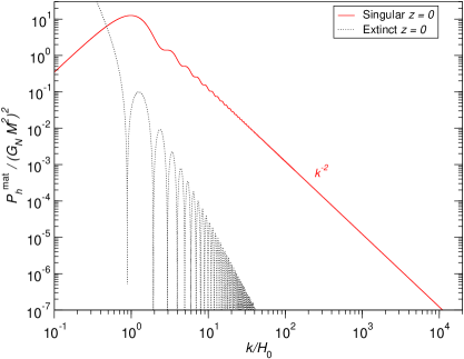
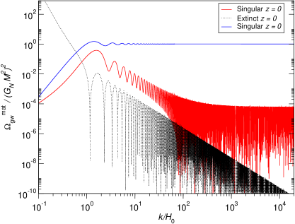
Figure 5: The left panel shows the normalised strain power spectrum $\mathcal{P}_{h}^{\mathrm{mat}}/(G_{\mathrm{{\scriptscriptstyle{N}}}}M^{2})^{2}$ generated in the matter era by a singular source having a correlator $\mathcal{U}(x,x^{\prime})=\mathcal{U}_{\infty}/\sqrt{xx^{\prime}}$ (red curve). It is compared to the one associated with extinct sources (black dotted curve). Notice the unusual behaviour of $k^{2}\mathcal{P}_{h}^{\mathrm{mat}}$ becoming scale invariant at large wavenumbers. The right panel shows the corresponding energy density parameter $\Omega_{\mathrm{gw}}^{\mathrm{mat}}/(G_{\mathrm{{\scriptscriptstyle{N}}}}M^{2})^{2}$, coming from the singular source in red, associated with extinct sources in black (dotted curve) and compared to the singular $k^{2}/(12\mathcal{H}_{0}^{2})\mathcal{P}_{h}^{\mathrm{mat}}$ (blue horizontal curve). The usual relation $\Omega_{\mathrm{gw}}^{\mathrm{mat}}\simeq k^{2}/(12\mathcal{H}_{0}^{2})\mathcal{P}_{h}$ is violated on all length scales. For illustration purposes, we have set $\mathcal{U}_{\infty}=1$.

We have represented in figure 5 the shape of the equal-time matter era spectra coming from the singular correlator and compared them to the ones associated with the extinct sources. In the right panel of this figure, both $\Omega_{\mathrm{gw}}^{\mathrm{mat}}$ and $k^{2}/(12\mathcal{H}_{0}^{2})\mathcal{P}_{h}^{\mathrm{mat}}$ are represented. They strongly differ at all wavenumbers. The perfectly coherent correlator of equation (3.63) exhibits a high degree of symmetry and decreases very slowly as $1/\sqrt{x}$ at fixed $x^{\prime}$. But the main reason for the appearance of the singular behaviour described above lies in the fact that the function $\mathcal{C}_{k}(y,y^{\prime})$ is not square integrable, and this statement depends not only on how the correlator $\mathcal{U}(x,x^{\prime})$ behaves at large $(x,x^{\prime})$ but also on how fast the scale factor $a(\eta)$ grows. That is why the singular spectra associated with equation (3.63) exhibit more pronounced differences with respect to the extinct sources case in the matter era than in the radiation era. Concerning the choice of a coherent correlator, one could easily check that a perfectly incoherent correlator, varying as $\mathcal{U}(x,x^{\prime})=\mathcal{U}_{\infty}\delta(x-x^{\prime})/x$ would induce an even more pronounced effect in the matter era, the strain power spectrum decreasing only as $1/k$ at large wavenumbers (the Dirac distribution makes it more singular). One can also check that smoothing the transverse structure of the correlator with some Gaussian function does not change the result. In figure 6, we have represented the matter era strain power spectrum numerically computed from a smoothed correlator varying as

$$\mathcal{U}^{\mathrm{mat}}(x,x^{\prime})=\dfrac{\mathcal{U}_{\infty}^{\mathrm{mat}}}{\sqrt{xx^{\prime}}}\exp\left[-\dfrac{\left(\frac{x}{x^{\prime}}-1\right)^{2}}{2\sigma^{2}}\right],$$ (3.84)

and for various values of $\sigma$. The effect of having a strong smoothing $\sigma\ll 1$ is to damp the oscillations visible in figure 5, add a new correlation scale in the spectrum around $k\simeq 1/\sigma$, but the slow decay of $\mathcal{P}_{h}^{\mathrm{mat}}\propto 1/k^{2}$ at large wavenumbers remains. In conclusion, the simplest way to determine if any singular behaviour is present is to search for singularities in the Fourier transform $\hat{\mathcal{C}}_{k}(\gamma,\gamma^{\prime})$. When $\mathcal{C}_{k}(x,x^{\prime})$ is non-square integrable, poles are expected to show up at null “frequencies” $(\gamma,\gamma^{\prime})$, but any other singularities elsewhere would equally trigger new features in the spectrum and deviations from the extinct sources case.

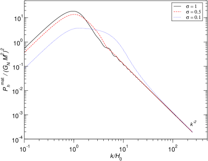
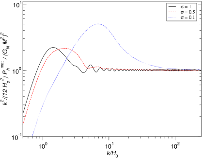
Figure 6: Direct numerical evaluation of the normalised strain power spectrum $\mathcal{P}_{h}^{\mathrm{mat}}/(G_{\mathrm{{\scriptscriptstyle{N}}}}M^{2})^{2}$ (left panel) generated in the matter era by the smoothed singular source of equation (3.84) (with $\mathcal{U}_{\infty}^{\mathrm{mat}}=1$), for different values of the smoothing width $\sigma$. The right panel shows the rescaled spectrum $k^{2}/(12\mathcal{H}_{0}^{2})\mathcal{P}_{h}^{\mathrm{mat}}/(G_{\mathrm{{\scriptscriptstyle{N}}}}M^{2})^{2}$. The smoothing does not affect the behaviour at large wavenumbers $\mathcal{P}_{h}^{\mathrm{mat}}\propto 1/k^{2}$ (see also figure 5).

A note of caution is however in order. All along the paper we have considered an instantaneous transition from the radiation to the matter era and we have assumed that the anisotropic stress could take a scaling form instantaneously at the transition. All realistic scaling sources are expected to not being in “scaling” during the transition and various distortions on the spectra should be expected around the length scales associated $k=1/\eta_{\mathrm{eq}}$. For instance, it is perfectly possible that the matter era power spectrum associated with cosmic strings exhibit the $1/k^{2}$ decrease (see figure 5) only over an intermediate range of wavenumbers above which it could be sensitive to the non-scaling anisotropic stress at $k>1/\eta_{\mathrm{eq}}$. Only a full numerical simulation of cosmic strings would allow us to determine its precise shape [41].

4 Conclusion

Let us briefly recap our main results. We have derived the explicit unequal-time and wavenumber dependence of the strain power spectrum $\mathcal{P}_{h}(\eta_{1},\eta_{2},k)$ as well as the energy density parameter $\Omega_{\mathrm{gw}}(\eta_{1},\eta_{2},k)$ for scaling sources. For a wide class of sources, extinct and smooth, having a holomorphic Fourier transform $\hat{\mathcal{C}}_{k}(\gamma,\gamma^{\prime})$, we have derived their complete analytical forms given in equations (3.40), (3.41), (3.45), (3.46), (3.49) and (B.4). However, realistic scaling sources are expected to be “constant” on large scales before turning “extinct” on smaller scales. The spectra for constant sources have been derived in section 3.6 and exhibit only small modulations. As such, realistic sources may only be strongly oscillating at small scales, in a regime which is notoriously difficult to compute, but on immediate reach by GW direct detection experiments. Let us notice that other cosmological sources, not necessarily scaling, have been shown to produce oscillations [51, 52, 53] or time variation [54]. The precise determination of the SGWB fine structure is therefore of immediate interest for their disambiguation. In section 3.7, we have discussed a counter-example of extinct sources that we refer to as a singular source. It mimics the behaviour of long cosmic strings at small scales and the function $\hat{\mathcal{C}}_{k}(\gamma,\gamma^{\prime})$ is no longer holomorphic. This results in various drastic changes in the oscillatory structure of both the strain and energy density spectra that would allow its disambiguation from extinct sources. Interestingly such a case provides an example for which only the presence of interferences on top of the fine structure would allow for a clear disambiguation between the radiation-era generated spectra. In the matter era, we have found strong changes, such as a very slow decay of $\mathcal{P}_{h}^{\mathrm{mat}}\propto 1/k^{2}$ (instead of the expected $1/k^{4}$) and a violation of the relation $\Omega_{\mathrm{gw}}\simeq k^{2}/(12\mathcal{H}^{2})\mathcal{P}_{h}$ for all wavenumbers.

These results have various implications. One is that there is no reason for cosmological predictions to use $\Omega_{\mathrm{gw}}(\eta_{1},\eta_{2},k)$ as a proxy, being the two-point correlation function of $h_{ij}^{\prime}$ it is not the quantity of interest for direct measurements which are sensitive to correlations in the strain. As we have shown, both quantities can be significantly different for the singular sources and this could be a source of errors in the predictions. The only usage of $\Omega_{\mathrm{gw}}$ should be in measuring the overall gravitating effect of gravitational waves, as it is done during BBN for instance. Another implication concerns the waveform measurable by direct detection experiments. Our results are given in spatial Fourier space, with time-dependent terms. Taking the inverse spatial Fourier transform of our formulas as well as the forward Fourier transform with respect to the time $\eta$ would give a function of spatial separation ${\boldsymbol{x}}$ and angular frequency $\omega$. The fine structure in $k$ implies that the correlators have also some fine structure in ${\boldsymbol{x}}$ and it would be interesting to determine how the signal changes with respect to the separation between the interferometers. Concerning the angular frequencies, at fixed wavenumber $k$, only four are excited $\omega=\pm k$ and $\omega=\pm 2k$. This is expected, we consider correlators which are the square of the strain, this one being a superimposition of free waves having $\omega=k$ and $\omega=-k$. However, the amplitude of each of these four oscillatory terms is peculiar to each type of source and its experimental determination would be interesting. Concerning cosmic strings, let us recap that most of the overall GW emission is expected to come from cosmic string loops and not from long strings, at least for Nambu-Goto strings. Moreover, even if the matter era spectrum $\mathcal{P}_{h}\propto 1/k^{2}$ instead of $1/k^{4}$, it is perfectly possible that this effect remain completely negligible because the long strings contribution from the radiation era is also varying as $1/k^{2}$, and, it could be the dominating part. However, this is of clear interest for models in which cosmic strings are formed during inflation and would enter scaling only in the matter era [55, 56, 57]. In view of our results, these models could be constrained by GW direct detection experiments.

Finally, it would be interesting to search for a generalisation of the case of extinct sources, out of the scaling hypothesis. For instance, it should be possible to extend the results derived for holomorphic anisotropic stresses to explicit time-dependent sources provided they can be factorized with some “scaling terms”. We let however these investigations for a future work.

Appendix A Holomorphic correlators in Fourier space

In this appendix, we rigorously derive the value of the integrals $I_{\mathrm{cc}}$, $I_{\mathrm{ss}}$, $I_{\mathrm{cs}}$ and $I_{\mathrm{sc}}$ presented in the section 3.4 when the Fourier transform of the correlator $\hat{\mathcal{C}}_{k}(\gamma,\gamma^{\prime})$ is a holomorphic function.

Let us explain the method with equation (3.29). Expanding the sine cardinal functions into complex exponentials, we can rewrite $I_{\mathrm{cc}}$ as

$$I_{\mathrm{cc}}=-\dfrac{1}{16\pi^{2}}\iint_{-\infty}^{+\infty}\mathrm{d}\gamma\mathrm{d}\gamma^{\prime}\left[e^{\imath(1-\gamma)y_{1}}-e^{-\imath(1-\gamma)y_{1}}\right]\left[e^{\imath(1-\gamma^{\prime})y_{2}}-e^{-\imath(1-\gamma^{\prime})y_{2}}\right]\dfrac{\hat{\mathcal{C}}_{k}(\gamma,\gamma^{\prime})}{(1-\gamma)(1-\gamma^{\prime})}\,,$$ (A.1)

where the “natural” poles in $\gamma=1$ and $\gamma^{\prime}=1$ coming from GW propagation are now made explicit. Expanding all terms give

$$I_{\mathrm{cc}} =-\dfrac{1}{4}\Bigg{\{}e^{\imath(y_{1}+y_{2})}\mathcal{F}^{-1}\!\left[\dfrac{\hat{\mathcal{C}}_{k}(-\gamma,-\gamma^{\prime})}{(1+\gamma)(1+\gamma^{\prime})}\right]-e^{\imath(y_{1}-y_{2})}\mathcal{F}^{-1}\!\left[\dfrac{\hat{\mathcal{C}}_{k}(-\gamma,\gamma^{\prime})}{(1+\gamma)(1-\gamma^{\prime})}\right]$$ (A.2)

$$-e^{-i(y_{1}-y_{2})}\mathcal{F}^{-1}\!\left[\dfrac{\hat{\mathcal{C}}_{k}(\gamma,-\gamma^{\prime})}{(1-\gamma)(1+\gamma^{\prime})}\right]+e^{-i(y_{1}+y_{2})}\mathcal{F}^{-1}\!\left[\dfrac{\hat{\mathcal{C}}_{k}(\gamma,\gamma^{\prime})}{(1-\gamma)(1-\gamma^{\prime})}\right]\Bigg{\}},$$

where $\mathcal{F}^{-1}\!\left(\right)$ denotes the inverse Fourier transform, going from $(\gamma,\gamma^{\prime})$ to $(y_{1},y_{2})$. The expression of $I_{\mathrm{cc}}$ is known if one can evaluate these inverse Fourier transforms, and they are trivial provided the function $\hat{\mathcal{C}}_{k}(\gamma,\gamma^{\prime})$ is holomorphic. Let us focus on

$$\mathcal{F}^{-1}\!\left[\dfrac{\hat{\mathcal{C}}_{k}(-\gamma,-\gamma^{\prime})}{(1+\gamma)(1+\gamma^{\prime})}\right]=\dfrac{1}{4\pi^{2}}\int_{-\infty}^{+\infty}\mathrm{d}\gamma^{\prime}\dfrac{e^{\imath\gamma^{\prime}y_{2}}}{1+\gamma^{\prime}}\int_{-\infty}^{+\infty}\mathrm{d}\gamma\dfrac{\hat{\mathcal{C}}_{k}(-\gamma,-\gamma^{\prime})}{1+\gamma}e^{\imath\gamma y_{1}}.$$ (A.3)

The simple pole at $\gamma=-1$ in the last integral requires an integration contour to be chosen in the complex plane to determine its Cauchy principal value. This one is depicted in figure 7. After pushing the upper contour to complex infinity and the smaller one towards the pole, one finds

$$\int_{-\infty}^{+\infty}\mathrm{d}\gamma\dfrac{\hat{\mathcal{C}}_{k}(-\gamma,-\gamma^{\prime})}{1+\gamma}e^{\imath\gamma y_{1}}=\imath\pi e^{-\imath y_{1}}\hat{\mathcal{C}}_{k}(1,-\gamma^{\prime}).$$ (A.4)

Figure 7: Integration contour used to evaluate the inverse Fourier transform of equation (A.3).

Repeating the same procedure for the remaining integral in equation (A.3), in the complex plane $[\Re(\gamma^{\prime}),\Im(\gamma^{\prime})]$, we get

$$\mathcal{F}^{-1}\!\left[\dfrac{\hat{\mathcal{C}}_{k}(-\gamma,-\gamma^{\prime})}{(1+\gamma)(1+\gamma^{\prime})}\right]=-\dfrac{1}{4}e^{-\imath(y_{1}+y_{2})}\hat{\mathcal{C}}_{k}(1,1).$$ (A.5)

The other inverse Fourier transforms appearing in equation (A.2) can be dealt in the same way. Notice however that the poles are not at the exact same location, they are in $\gamma=\pm 1$ and $\gamma^{\prime}=\pm 1$. We obtain

$$\mathcal{F}^{-1}\!\left[\dfrac{\hat{\mathcal{C}}_{k}(-\gamma,\gamma^{\prime})}{(1+\gamma)(1-\gamma^{\prime})}\right] =+\dfrac{1}{4}e^{-\imath(y_{1}-y_{2})}\hat{\mathcal{C}}_{k}(1,1),$$ (A.6)

$$\mathcal{F}^{-1}\!\left[\dfrac{\hat{\mathcal{C}}_{k}(\gamma,-\gamma^{\prime})}{(1-\gamma)(1+\gamma^{\prime})}\right] =+\dfrac{1}{4}e^{\imath(y_{1}-y_{2})}\hat{\mathcal{C}}_{k}(1,1),$$

$$\mathcal{F}^{-1}\!\left[\dfrac{\hat{\mathcal{C}}_{k}(\gamma,\gamma^{\prime})}{(1-\gamma)(1-\gamma^{\prime})}\right] =-\dfrac{1}{4}e^{\imath(y_{1}+y_{2})}\hat{\mathcal{C}}_{k}(1,1),$$

from which equation (A.2) gives

$$I_{\mathrm{cc}}=\dfrac{1}{4}\hat{\mathcal{C}}_{k}(1,1).$$ (A.7)

The other integrals $I_{\mathrm{ss}}$, $I_{\mathrm{cs}}$ and $I_{\mathrm{sc}}$ can be explicitly calculated with the same method. However, because they involve functions of the form $\operatorname{sinc}^{2}[(1-\gamma)y_{1}/2]$, when doing an expansion in terms of complex exponentials, constant terms appear and one has to evaluate three new integrals. Two of them are one-dimensional inverse Fourier transforms

$$I_{1}=\dfrac{1}{2}\mathcal{F}^{-1}\!\left[\dfrac{\hat{\mathcal{C}}(\gamma,1)}{1-\gamma}\right]_{y_{1}=0},\qquad I_{1}^{\prime}=\dfrac{1}{2}\mathcal{F}^{-1}\!\left[\dfrac{\hat{\mathcal{C}}(1,\gamma^{\prime})}{1-\gamma^{\prime}}\right]_{y_{2}=0},$$ (A.8)

and the last one is the two-dimensional inverse Fourier transform

$$I_{2}=\mathcal{F}^{-1}\!\left[\dfrac{\hat{\mathcal{C}}(\gamma,\gamma^{\prime})}{(1-\gamma)(1-\gamma^{\prime})}\right]_{(y_{1},y_{2})=(0,0)},$$ (A.9)

all evaluated at the origin. To calculate their value one can make use of the Dirichlet’s theorem and evaluate the integrals at $y_{1}=0^{\pm}$ and $y_{2}=0^{\pm}$. Each sign requiring a different integration contour. Taking the mean finally gives $I_{1}=I_{1}^{\prime}=I_{2}=0$ which propagates to $I_{\mathrm{ss}}=I_{\mathrm{cs}}=I_{\mathrm{sc}}=0$ as stated in section 3.4.

Appendix B Spectra from extinct sources

As described in section 3.4.3, the calculation of the integral $I_{\mu}^{\mathrm{mat}}$ proceeds exactly as the one detailed for the radiation era but starting from the matter era convolution kernels given in equation (3.5). From equation (3.4), using the definitions (3.47) and (3.48), one gets, for extinct sources in the matter era,

$$I_{\mu}^{\mathrm{mat}}(x_{1},x_{2},k)=\dfrac{\hat{\mathcal{C}}_{k}^{\mathrm{mat}}+\hat{\mathcal{E}}_{k}^{\mathrm{mat}}}{8}\dfrac{1+(x_{1}+x_{\mathrm{eq}})(x_{2}+x_{\mathrm{eq}})}{(x_{1}+x_{\mathrm{eq}})(x_{2}+x_{\mathrm{eq}})}\cos(x_{1}-x_{2})$$

$$+\dfrac{\hat{\mathcal{C}}_{k}^{\mathrm{mat}}+\hat{\mathcal{E}}_{k}^{\mathrm{mat}}}{8}\dfrac{x_{1}-x_{2}}{(x_{1}+x_{\mathrm{eq}})(x_{2}+x_{\mathrm{eq}})}\sin(x_{1}-x_{2})$$

$$+\dfrac{(\hat{\mathcal{C}}_{k}^{\mathrm{mat}}-\hat{\mathcal{E}}_{k}^{\mathrm{mat}})\left[1-(x_{1}+x_{\mathrm{eq}})(x_{2}+x_{\mathrm{eq}})\right]-2\hat{\mathcal{D}}_{k}^{\mathrm{mat}}(x_{1}+x_{2}+2x_{\mathrm{eq}})}{8(x_{1}+x_{\mathrm{eq}})(x_{2}+x_{\mathrm{eq}})}\cos(x_{1}+x_{2}-2x_{\mathrm{eq}})$$

$$+\dfrac{(\hat{\mathcal{C}}_{k}^{\mathrm{mat}}-\hat{\mathcal{E}}_{k}^{\mathrm{mat}})(x_{1}+x_{2}+2x_{\mathrm{eq}})+2\hat{\mathcal{D}}_{k}^{\mathrm{mat}}\left[1-(x_{1}+x_{\mathrm{eq}})(x_{2}+x_{\mathrm{eq}})\right]}{8(x_{1}+x_{\mathrm{eq}})(x_{2}+x_{\mathrm{eq}})}\sin(x_{1}+x_{2}-2x_{\mathrm{eq}}).$$ (B.1)

where we have used the abridged notation $\hat{\mathcal{C}}_{k}=\hat{\mathcal{C}}_{k}(1,1)$, $\hat{\mathcal{D}}_{k}=\hat{\mathcal{D}}_{k}(1,1)$ and $\hat{\mathcal{E}}_{k}=\hat{\mathcal{E}}_{k}(1,1)$. Plugging this expression into equation (3.3) gives the exact waveform of the unequal time strain power spectrum given in equation (3.49). The other integrals, $I_{\mu^{\prime}}^{\mathrm{mat}}$ and $I_{\kappa}^{\mathrm{mat}}$, entering the expression of $\Omega_{\mathrm{gw}}^{\mathrm{mat}}$, can be immediately obtained by using equation (3.20), i.e., by deriving the above expression with respect to $x_{1}$ and $x_{2}$. After lengthy algebra, one obtains

$$I_{\mu^{\prime}}^{\mathrm{mat}}(x_{1},x_{2},k)=\dfrac{\hat{\mathcal{C}}_{k}^{\mathrm{mat}}+\hat{\mathcal{E}}_{k}^{\mathrm{mat}}}{8(x_{1}+x_{\mathrm{eq}})^{2}(x_{2}+x_{\mathrm{eq}})^{2}}\left[1-x_{1}^{2}-x_{2}^{2}+x_{1}x_{2}(1+x_{1}x_{2})\right.$$

$$\left.+(x_{1}+x_{2})(2x_{1}x_{2}-1)x_{\mathrm{eq}}+(x_{1}^{2}-1+4x_{1}x_{2}+x_{2}^{2})x_{\mathrm{eq}}^{2}+2(x_{1}+x_{2})x_{\mathrm{eq}}^{3}+x_{\mathrm{eq}}^{4}\right]\cos(x_{1}-x_{2})$$

$$+\dfrac{\hat{\mathcal{C}}_{k}^{\mathrm{mat}}+\hat{\mathcal{E}}_{k}^{\mathrm{mat}}}{8(x_{1}+x_{\mathrm{eq}})^{2}(x_{2}+x_{\mathrm{eq}})^{2}}(x_{1}-x_{2})\left[1+(x_{1}+x_{\mathrm{eq}})(x_{2}+x_{\mathrm{eq}})\right]\sin(x_{1}-x_{2})$$

$$+\bigg{\{}\dfrac{\hat{\mathcal{C}}_{k}^{\mathrm{mat}}-\hat{\mathcal{E}}_{k}^{\mathrm{mat}}}{8(x_{1}+x_{\mathrm{eq}})^{2}(x_{2}+x_{\mathrm{eq}})^{2}}\left[1-(x_{1}+x_{\mathrm{eq}})^{2}-(x_{2}+x_{\mathrm{eq}})^{2}-(x_{1}+x_{\mathrm{eq}})(x_{2}+x_{\mathrm{eq}})\right.$$

$$\left.+(x_{1}+x_{\mathrm{eq}})^{2}(x_{2}+x_{\mathrm{eq}})^{2}\right]-\dfrac{\hat{\mathcal{D}}_{k}^{\mathrm{mat}}}{4}\dfrac{(x_{1}+x_{2}+2x_{\mathrm{eq}})\left[1-(x_{1}+x_{\mathrm{eq}})(x_{2}+x_{\mathrm{eq}})\right]}{(x_{1}+x_{\mathrm{eq}})^{2}(x_{2}+x_{\mathrm{eq}})^{2}}\bigg{\}}$$

$$\times\cos(x_{1}+x_{2}-2x_{\mathrm{eq}})$$

$$+\bigg{\{}\dfrac{\hat{\mathcal{C}}_{k}^{\mathrm{mat}}-\hat{\mathcal{E}}_{k}^{\mathrm{mat}}}{8}\dfrac{(x_{1}+x_{2}+2x_{\mathrm{eq}})\left[1-(x_{1}+x_{\mathrm{eq}})(x_{2}+x_{\mathrm{eq}})\right]}{(x_{1}+x_{\mathrm{eq}})^{2}(x_{2}+x_{\mathrm{eq}})^{2}}+\dfrac{\hat{\mathcal{D}}_{k}^{\mathrm{mat}}}{4(x_{1}+x_{\mathrm{eq}})^{2}(x_{2}+x_{\mathrm{eq}})^{2}}$$

$$\times\left[1-x_{1}^{2}-x_{2}^{2}-x_{1}x_{2}(1-x_{1}x_{2})+(x_{1}+x_{2})(2x_{1}x_{2}-3)x_{\mathrm{eq}}-(3-x_{1}^{2}-x_{2}^{2}-4x_{1}x_{2})x_{\mathrm{eq}}^{2}\right.$$

$$\left.+2(x_{1}+x_{2})x_{\mathrm{eq}}^{3}+x_{\mathrm{eq}}^{4}\right]\bigg{\}}\sin(x_{1}+x_{2}-2x_{\mathrm{eq}}),$$ (B.2)

and

$$I_{\kappa}^{\mathrm{mat}}(x_{1},x_{2},k)=\dfrac{\hat{\mathcal{C}}_{k}^{\mathrm{mat}}+\hat{\mathcal{E}}_{k}^{\mathrm{mat}}}{8}\dfrac{(x_{1}-x_{2})(x_{1}+x_{\mathrm{eq}})-1}{(x_{1}+x_{\mathrm{eq}})^{2}(x_{2}+x_{\mathrm{eq}})}\cos(x_{1}-x_{2})$$

$$-\dfrac{\hat{\mathcal{C}}_{k}^{\mathrm{mat}}+\hat{\mathcal{E}}_{k}^{\mathrm{mat}}}{8}\dfrac{x_{\mathrm{eq}}^{3}+x_{1}^{2}(x_{2}+x_{\mathrm{eq}})+x_{2}(x_{\mathrm{eq}}^{2}-1)+x_{1}(1+2x_{2}x_{\mathrm{eq}}+2x_{\mathrm{eq}}^{2})}{(x_{1}+x_{\mathrm{eq}})^{2}(x_{2}+x_{\mathrm{eq}})}\sin(x_{1}-x_{2})$$

$$+\bigg{\{}\dfrac{\hat{\mathcal{C}}_{k}^{\mathrm{mat}}-\hat{\mathcal{E}}_{k}^{\mathrm{mat}}}{8}\dfrac{x_{1}^{2}-1+x_{2}x_{\mathrm{eq}}+2x_{\mathrm{eq}}^{2}+x_{1}(x_{2}+3x_{\mathrm{eq}})}{(x_{1}+x_{\mathrm{eq}})^{2}(x_{2}+x_{\mathrm{eq}})}+\dfrac{\hat{\mathcal{D}}_{k}^{\mathrm{mat}}}{4(x_{1}+x_{\mathrm{eq}})^{2}(x_{2}+x_{\mathrm{eq}})}\left[x_{1}+x_{2}\right.$$

$$\left.+2x_{\mathrm{eq}}-x_{2}x_{\mathrm{eq}}^{2}-x_{\mathrm{eq}}^{3}-x_{1}^{2}(x_{2}+x_{\mathrm{eq}})-2x_{1}x_{\mathrm{eq}}(x_{2}+x_{\mathrm{eq}})\right]\bigg{\}}\cos(x_{1}+x_{2}-2x_{\mathrm{eq}})$$

$$+\bigg{\{}-\dfrac{\hat{\mathcal{C}}_{k}^{\mathrm{mat}}-\hat{\mathcal{E}}_{k}^{\mathrm{mat}}}{8(x_{1}+x_{\mathrm{eq}})^{2}(x_{2}+x_{\mathrm{eq}})}\left[x_{1}+x_{2}+2x_{\mathrm{eq}}-x_{2}x_{\mathrm{eq}}^{2}-x_{\mathrm{eq}}^{3}-x_{1}^{2}(x_{2}+x_{\mathrm{eq}})\right.$$

$$\left.-2x_{1}x_{\mathrm{eq}}(x_{2}+x_{\mathrm{eq}})\right]+\dfrac{\hat{\mathcal{D}}_{k}^{\mathrm{mat}}}{4}\dfrac{x_{1}^{2}-1+x_{2}x_{\mathrm{eq}}+2x_{\mathrm{eq}}^{2}+x_{1}(x_{2}+3x_{\mathrm{eq}})}{(x_{1}+x_{\mathrm{eq}})^{2}(x_{2}+x_{\mathrm{eq}})}\bigg{\}}\sin(x_{1}+x_{2}-2x_{\mathrm{eq}}).$$ (B.3)

The last integral, $I_{\bar{\kappa}}(x_{1},x_{2},k)$, defined by equation (3.15), is obtained by complex conjugating the Fourier transformed correlators while swapping $x_{1}$ and $x_{2}$. For $\mathcal{U}(x,x^{\prime})$ symmetric, the $\mathcal{C}(y,y^{\prime})$, $\mathcal{D}(y,y^{\prime})$ and $\mathcal{E}(y,y^{\prime})$ functions are even, and real, such that their Fourier transform are also even and real. Therefore, it is enough to simply swap $x_{1}$ and $x_{2}$ in the previous expression to obtains $I_{\bar{\kappa}}$. Plugging equations (B.1) to (B.3) into the expression (3.12) one gets for the energy density parameter

$$\dfrac{\Omega_{\mathrm{gw}}^{\mathrm{mat}}(\eta_{1},\eta_{2},k)}{\dfrac{4}{3}\left(G_{\mathrm{{\scriptscriptstyle{N}}}}M^{2}\right)^{2}}=\left(\hat{\mathcal{C}}_{k}^{\mathrm{mat}}+\hat{\mathcal{E}}_{k}^{\mathrm{mat}}\right)\left[\dfrac{1+(x_{1}+x_{\mathrm{eq}})(x_{2}+x_{\mathrm{eq}})}{(x_{1}+x_{\mathrm{eq}})(x_{2}+x_{\mathrm{eq}})}\right.$$

$$\left.+\dfrac{k}{\mathcal{H}_{1}}\dfrac{1-(x_{1}+x_{\mathrm{eq}})^{2}+(x_{1}+x_{\mathrm{eq}})(x_{2}+x_{\mathrm{eq}})}{(x_{1}+x_{\mathrm{eq}})^{2}(x_{2}+x_{\mathrm{eq}})}+\dfrac{k}{\mathcal{H}_{2}}\dfrac{1+(x_{1}+x_{\mathrm{eq}})(x_{2}+x_{\mathrm{eq}})-(x_{2}+x_{\mathrm{eq}})^{2}}{(x_{1}+x_{\mathrm{eq}})(x_{2}+x_{\mathrm{eq}})^{2}}\right.$$

$$\left.+\dfrac{k^{2}}{\mathcal{H}_{1}\mathcal{H}_{2}}\dfrac{1+(x_{1}+x_{\mathrm{eq}})(x_{2}+x_{\mathrm{eq}})-(x_{2}+x_{\mathrm{eq}})^{2}-(x_{1}+x_{\mathrm{eq}})^{2}+(x_{1}+x_{\mathrm{eq}})^{2}(x_{2}+x_{\mathrm{eq}})^{2}}{(x_{1}+x_{\mathrm{eq}})^{2}(x_{2}+x_{\mathrm{eq}})^{2}}\right]$$

$$\times\cos(x_{1}-x_{2})$$

$$+\left(\hat{\mathcal{C}}_{k}^{\mathrm{mat}}+\hat{\mathcal{E}}_{k}^{\mathrm{mat}}\right)\left[\dfrac{x_{1}-x_{2}}{(x_{1}+x_{\mathrm{eq}})(x_{2}+x_{\mathrm{eq}})}+\dfrac{k}{\mathcal{H}_{1}}\dfrac{x_{1}-x_{2}+(x_{1}+x_{\mathrm{eq}})^{2}(x_{2}+x_{\mathrm{eq}})}{(x_{1}+x_{\mathrm{eq}})^{2}(x_{2}+x_{\mathrm{eq}})}\right.$$

$$\left.+\dfrac{k}{\mathcal{H}_{2}}\dfrac{x_{1}-x_{2}-(x_{1}+x_{\mathrm{eq}})(x_{2}+x_{\mathrm{eq}})^{2}}{(x_{1}+x_{\mathrm{eq}})(x_{2}+x_{\mathrm{eq}})^{2}}\right.$$

$$\left.+\dfrac{k^{2}}{\mathcal{H}_{1}\mathcal{H}_{2}}\dfrac{x_{1}-x_{2}+(x_{1}+x_{\mathrm{eq}})^{2}(x_{2}+x_{\mathrm{eq}})-(x_{1}+x_{\mathrm{eq}})(x_{2}+x_{\mathrm{eq}})^{2}}{(x_{1}+x_{\mathrm{eq}})^{2}(x_{2}+x_{\mathrm{eq}})^{2}}\right]\sin(x_{1}-x_{2})$$

$$+\bigg{\{}\left(\hat{\mathcal{C}}_{k}^{\mathrm{mat}}-\hat{\mathcal{E}}_{k}^{\mathrm{mat}}\right)\left[-1+\dfrac{1}{(x_{1}+x_{\mathrm{eq}})(x_{2}+x_{\mathrm{eq}})}\right]-2\hat{\mathcal{D}}_{k}^{\mathrm{mat}}\dfrac{x_{1}+x_{2}+2x_{\mathrm{eq}}}{(x_{1}+x_{\mathrm{eq}})(x_{2}+x_{\mathrm{eq}})}$$

$$+\dfrac{k}{\mathcal{H}_{1}}\left[\left(\hat{\mathcal{C}}_{k}^{\mathrm{mat}}-\hat{\mathcal{E}}_{k}^{\mathrm{mat}}\right)\dfrac{1-(x_{1}+x_{\mathrm{eq}})^{2}-(x_{1}+x_{\mathrm{eq}})(x_{2}+x_{\mathrm{eq}})}{(x_{1}+x_{\mathrm{eq}})^{2}(x_{2}+x_{\mathrm{eq}})}\right.$$

$$\left.-2\hat{\mathcal{D}}_{k}^{\mathrm{mat}}\dfrac{x_{1}+x_{2}+2x_{\mathrm{eq}}-(x_{1}+x_{\mathrm{eq}})^{2}(x_{2}+x_{\mathrm{eq}})}{(x_{1}+x_{\mathrm{eq}})^{2}(x_{2}+x_{\mathrm{eq}})}\right]$$

$$+\dfrac{k}{\mathcal{H}_{2}}\left[\left(\hat{\mathcal{C}}_{k}^{\mathrm{mat}}-\hat{\mathcal{E}}_{k}^{\mathrm{mat}}\right)\dfrac{1-(x_{2}+x_{\mathrm{eq}})^{2}-(x_{1}+x_{\mathrm{eq}})(x_{2}+x_{\mathrm{eq}})}{(x_{1}+x_{\mathrm{eq}})(x_{2}+x_{\mathrm{eq}})^{2}}\right.$$

$$\left.-2\hat{\mathcal{D}}_{k}^{\mathrm{mat}}\dfrac{x_{1}+x_{2}+2x_{\mathrm{eq}}-(x_{1}+x_{\mathrm{eq}})(x_{2}+x_{\mathrm{eq}})^{2}}{(x_{1}+x_{\mathrm{eq}})(x_{2}+x_{\mathrm{eq}})^{2}}\right]$$

$$+\dfrac{k^{2}}{\mathcal{H}_{1}\mathcal{H}_{2}}\left[-2\hat{\mathcal{D}}_{k}^{\mathrm{mat}}\dfrac{x_{1}+x_{2}+2x_{\mathrm{eq}}-(x_{1}+x_{\mathrm{eq}})^{2}(x_{2}+x_{\mathrm{eq}})-(x_{1}+x_{\mathrm{eq}})(x_{2}+x_{\mathrm{eq}})^{2}}{(x_{1}+x_{\mathrm{eq}})^{2}(x_{2}+x_{\mathrm{eq}})^{2}}\right.$$

$$\left.+\dfrac{1-(x_{1}+x_{\mathrm{eq}})(x_{2}+x_{\mathrm{eq}})-(x_{1}+x_{\mathrm{eq}})^{2}-(x_{2}+x_{\mathrm{eq}})^{2}+(x_{1}+x_{\mathrm{eq}})^{2}(x_{2}+x_{\mathrm{eq}})^{2}}{(x_{1}+x_{\mathrm{eq}})^{2}(x_{2}+x_{\mathrm{eq}})^{2}}\right.$$

$$\left.\times\left(\hat{\mathcal{C}}_{k}^{\mathrm{mat}}-\hat{\mathcal{E}}_{k}^{\mathrm{mat}}\right)\right]\bigg{\}}\cos\left(x_{1}+x_{2}-2x_{\mathrm{eq}}\right)$$

$$+\bigg{\{}\left(\hat{\mathcal{C}}_{k}^{\mathrm{mat}}-\hat{\mathcal{E}}_{k}^{\mathrm{mat}}\right)\dfrac{x_{1}+x_{2}+2x_{\mathrm{eq}}}{(x_{1}+x_{\mathrm{eq}})(x_{2}+x_{\mathrm{eq}})}+2\hat{\mathcal{D}}_{k}^{\mathrm{mat}}\dfrac{1-(x_{1}+x_{\mathrm{eq}})(x_{2}+x_{\mathrm{eq}})}{(x_{1}+x_{\mathrm{eq}})(x_{2}+x_{\mathrm{eq}})}$$

$$+\dfrac{k}{\mathcal{H}_{1}}\left[\left(\hat{\mathcal{C}}_{k}^{\mathrm{mat}}-\hat{\mathcal{E}}_{k}^{\mathrm{mat}}\right)\dfrac{x_{1}+x_{2}+2x_{\mathrm{eq}}-(x_{1}+x_{\mathrm{eq}})^{2}(x_{2}+x_{\mathrm{eq}})}{(x_{1}+x_{\mathrm{eq}})^{2}(x_{2}+x_{\mathrm{eq}})}\right.$$

$$\left.+2\hat{\mathcal{D}}_{k}^{\mathrm{mat}}\dfrac{1-(x_{1}+x_{\mathrm{eq}})^{2}-(x_{1}+x_{\mathrm{eq}})(x_{2}+x_{\mathrm{eq}})}{(x_{1}+x_{\mathrm{eq}})^{2}(x_{2}+x_{\mathrm{eq}})}\right]$$

$$+\dfrac{k}{\mathcal{H}_{2}}\left[\left(\hat{\mathcal{C}}_{k}^{\mathrm{mat}}-\hat{\mathcal{E}}_{k}^{\mathrm{mat}}\right)\dfrac{x_{1}+x_{2}+2x_{\mathrm{eq}}-(x_{1}+x_{\mathrm{eq}})(x_{2}+x_{\mathrm{eq}})^{2}}{(x_{1}+x_{\mathrm{eq}})(x_{2}+x_{\mathrm{eq}})^{2}}\right.$$

$$\left.+2\hat{\mathcal{D}}_{k}^{\mathrm{mat}}\dfrac{1-(x_{1}+x_{\mathrm{eq}})(x_{2}+x_{\mathrm{eq}})-(x_{2}+x_{\mathrm{eq}})^{2}}{(x_{1}+x_{\mathrm{eq}})(x_{2}+x_{\mathrm{eq}})^{2}}\right]$$

$$+\dfrac{k^{2}}{\mathcal{H}_{1}\mathcal{H}_{2}}\left[\left(\hat{\mathcal{C}}_{k}^{\mathrm{mat}}-\hat{\mathcal{E}}_{k}^{\mathrm{mat}}\right)\dfrac{x_{1}+x_{2}+2x_{\mathrm{eq}}-(x_{1}+x_{\mathrm{eq}})^{2}(x_{2}+x_{\mathrm{eq}})-(x_{1}+x_{\mathrm{eq}})(x_{2}+x_{\mathrm{eq}})^{2}}{(x_{1}+x_{\mathrm{eq}})^{2}(x_{2}+x_{\mathrm{eq}})^{2}}\right.$$

$$\left.+2\hat{\mathcal{D}}_{k}^{\mathrm{mat}}\dfrac{1-(x_{1}+x_{\mathrm{eq}})(x_{2}+x_{\mathrm{eq}})-(x_{1}+x_{\mathrm{eq}})^{2}-(x_{2}+x_{\mathrm{eq}})^{2}+(x_{1}+x_{\mathrm{eq}})^{2}(x_{2}+x_{\mathrm{eq}})^{2}}{(x_{1}+x_{\mathrm{eq}})^{2}(x_{2}+x_{\mathrm{eq}})^{2}}\right]\bigg{\}}$$

$$\times\sin\left(x_{1}+x_{2}-2x_{\mathrm{eq}}\right).$$ (B.4)

References

- [1] G. Desvignes et al., High-precision timing of 42 millisecond pulsars with the European Pulsar Timing Array, Mon. Not. Roy. Astron. Soc. 458 (2016) 3341 [1602.08511].
- [2] B.B.P. Perera et al., The International Pulsar Timing Array: Second data release, Mon. Not. Roy. Astron. Soc. 490 (2019) 4666 [1909.04534].
- [3] NANOGrav collaboration, The NANOGrav 12.5 yr Data Set: Search for an Isotropic Stochastic Gravitational-wave Background, Astrophys. J. Lett. 905 (2020) L34 [2009.04496].
- [4] M. Kerr et al., The Parkes Pulsar Timing Array project: second data release, Publ. Astron. Soc. Austral. 37 (2020) e020 [2003.09780].
- [5] LIGO Scientific, Virgo, KAGRA collaboration, Upper Limits on the Isotropic Gravitational-Wave Background from Advanced LIGO’s and Advanced Virgo’s Third Observing Run, 2101.12130.
- [6] B. Allen, The Stochastic gravity wave background: Sources and detection, in Les Houches School of Physics: Astrophysical Sources of Gravitational Radiation, pp. 373–417, 4, 1996 [gr-qc/9604033].
- [7] N. Christensen, Stochastic Gravitational Wave Backgrounds, Rept. Prog. Phys. 82 (2019) 016903 [1811.08797].
- [8] C. Caprini and D.G. Figueroa, Cosmological Backgrounds of Gravitational Waves, Class. Quant. Grav. 35 (2018) 163001 [1801.04268].
- [9] S. Detweiler, Pulsar timing measurements and the search for gravitational waves, Astrophys. J. 234 (1979) 1100.
- [10] B.J. Carr, Cosmological gravitational waves - Their origin and consequences, Astron. Astrophys. 89 (1980) 6.
- [11] A. Vilenkin, Gravitation radiation from cosmic strings., Phys. Lett. B 107 (1981) 47.
- [12] B. Bertotti, B.J. Carr and M.J. Rees, Limits from the timing of pulsars on the cosmic gravitational wave background., Mon. Not. R. Astron. Soc. 203 (1983) 945.
- [13] C.J. Hogan and M.J. Rees, Gravitational interactions of cosmic strings, Nature 311 (1984) 109.
- [14] T. Vachaspati and A. Vilenkin, Gravitational Radiation from Cosmic Strings, Phys. Rev. D31 (1985) 3052.
- [15] F.S. Accetta and L.M. Krauss, The stochastic gravitational wave spectrum resulting from cosmic string evolution, Nucl. Phys. B319 (1989) 747.
- [16] D.P. Bennett and F.R. Bouchet, Constraints on the gravity wave background generated by cosmic strings, Phys. Rev. D43 (1991) 2733.
- [17] R.R. Caldwell and B. Allen, Cosmological constraints on cosmic string gravitational radiation, Phys. Rev. D45 (1992) 3447.
- [18] Planck collaboration, Planck 2018 results. VI. Cosmological parameters, Astron. Astrophys. 641 (2020) A6 [1807.06209].
- [19] B.D. Fields, K.A. Olive, T.-H. Yeh and C. Young, Big-Bang Nucleosynthesis after Planck, JCAP 03 (2020) 010 [1912.01132].
- [20] C. Pitrou, A. Coc, J.-P. Uzan and E. Vangioni, A new tension in the cosmological model from primordial deuterium?, Mon. Not. Roy. Astron. Soc. 502 (2021) 2474 [2011.11320].
- [21] M. Kamionkowski, A. Kosowsky and A. Stebbins, A Probe of primordial gravity waves and vorticity, Phys. Rev. Lett. 78 (1997) 2058 [astro-ph/9609132].
- [22] W. Hu, U. Seljak, M.J. White and M. Zaldarriaga, A complete treatment of CMB anisotropies in a FRW universe, Phys. Rev. D 57 (1998) 3290 [astro-ph/9709066].
- [23] Planck collaboration, Planck 2018 results. X. Constraints on inflation, Astron. Astrophys. 641 (2020) A10 [1807.06211].
- [24] SPTpol, BICEP, Keck collaboration, A demonstration of improved constraints on primordial gravitational waves with delensing, Phys. Rev. D 103 (2021) 022004 [2011.08163].
- [25] J.D. Romano and N.J. Cornish, Detection methods for stochastic gravitational-wave backgrounds: a unified treatment, Living Rev. Rel. 20 (2017) 2 [1608.06889].
- [26] C. Caprini, R. Durrer and R. Sturani, On the frequency of gravitational waves, Phys. Rev. D 74 (2006) 127501 [astro-ph/0607651].
- [27] C. Caprini, R. Durrer, T. Konstandin and G. Servant, General Properties of the Gravitational Wave Spectrum from Phase Transitions, Phys. Rev. D 79 (2009) 083519 [0901.1661].
- [28] C. Caprini, R. Durrer and G. Servant, The stochastic gravitational wave background from turbulence and magnetic fields generated by a first-order phase transition, JCAP 12 (2009) 024 [0909.0622].
- [29] M. Hindmarsh, C. Ringeval and T. Suyama, The CMB temperature bispectrum induced by cosmic strings, Phys. Rev. D80 (2009) 083501 [0908.0432].
- [30] D.G. Figueroa, M. Hindmarsh and J. Urrestilla, Exact Scale-Invariant Background of Gravitational Waves from Cosmic Defects, Phys. Rev. Lett. 110 (2013) 101302 [1212.5458].
- [31] D.G. Figueroa, M. Hindmarsh, J. Lizarraga and J. Urrestilla, Irreducible background of gravitational waves from a cosmic defect network: update and comparison of numerical techniques, Phys. Rev. D 102 (2020) 103516 [2007.03337].
- [32] M. Zaldarriaga and U. Seljak, An all sky analysis of polarization in the microwave background, Phys. Rev. D 55 (1997) 1830 [astro-ph/9609170].
- [33] S. Alexander and J. Martin, Birefringent gravitational waves and the consistency check of inflation, Phys. Rev. D 71 (2005) 063526 [hep-th/0410230].
- [34] V.F. Mukhanov, H.A. Feldman and R.H. Brandenberger, Theory of cosmological perturbations. part 1. classical perturbations. part 2. quantum theory of perturbations. part 3. extensions, Phys. Rept. 215 (1992) 203.
- [35] M. Abramowitz and I.A. Stegun, Handbook of mathematical functions with formulas, graphs, and mathematical tables, National Bureau of Standards, Washington, US, ninth ed. (1970).
- [36] N. Deruelle and V.F. Mukhanov, On matching conditions for cosmological perturbations, Phys. Rev. D 52 (1995) 5549 [gr-qc/9503050].
- [37] J. Martin and D.J. Schwarz, The Influence of cosmological transitions on the evolution of density perturbations, Phys. Rev. D 57 (1998) 3302 [gr-qc/9704049].
- [38] Y. Watanabe and E. Komatsu, Improved Calculation of the Primordial Gravitational Wave Spectrum in the Standard Model, Phys. Rev. D73 (2006) 123515 [astro-ph/0604176].
- [39] S. Kuroyanagi, C. Ringeval and T. Takahashi, Early universe tomography with CMB and gravitational waves, Phys. Rev. D87 (2013) 083502 [1301.1778].
- [40] L.D. Landau and E.M. Lifschits, Théorie des Champs, vol. 2, Mir Editions, Moscow (1989).
- [41] D. Camargo Neves da Cunha and C. Ringeval, In preparation (2021).
- [42] R. Durrer and M. Kunz, Cosmic microwave background anisotropies from scaling seeds: Generic properties of the correlation functions, Phys. Rev. D57 (1998) R3199 [astro-ph/9711133].
- [43] R. Durrer, M. Kunz and A. Melchiorri, Cosmic structure formation with topological defects, Phys. Rep. 364 (2002) 1 [astro-ph/0110348].
- [44] N. Bevis, M. Hindmarsh, M. Kunz and J. Urrestilla, Cmb power spectrum contribution from cosmic strings using field-evolution simulations of the abelian higgs model, Phys. Rev. D75 (2007) 065015 [astro-ph/0605018].
- [45] A. Lazanu, E. Shellard and M. Landriau, CMB power spectrum of Nambu-Goto cosmic strings, Phys. Rev. D91 (2015) 083519 [1410.4860].
- [46] N. Turok, Causality and the Doppler Peaks, Phys. Rev. D54 (1996) 3686 [astro-ph/9604172].
- [47] J.-H.P. Wu, P.P. Avelino, E.P.S. Shellard and B. Allen, Cosmic Strings, Loops, and Linear Growth of Matter Perturbations, Int. J. Mod. Phys. D 11 (2002) 61 [astro-ph/9812156].
- [48] B. Allen and E.P.S. Shellard, Gravitational radiation from cosmic strings, Phys. Rev. D 45 (1992) 1898.
- [49] A.A. Fraisse, C. Ringeval, D.N. Spergel and F.R. Bouchet, Small-Angle CMB Temperature Anisotropies Induced by Cosmic Strings, Phys. Rev. D78 (2008) 043535 [0708.1162].
- [50] C. Ringeval and F.R. Bouchet, All Sky CMB Map from Cosmic Strings Integrated Sachs-Wolfe Effect, Phys.Rev. D86 (2012) 023513 [1204.5041].
- [51] M. Kawasaki and K. Saikawa, Study of gravitational radiation from cosmic domain walls, JCAP 09 (2011) 008 [1102.5628].
- [52] S. Jung and T. Kim, Probing Cosmic Strings with Gravitational-Wave Fringe, JCAP 07 (2020) 068 [1810.04172].
- [53] J. Fumagalli, S. Renaux-Petel and L.T. Witkowski, Oscillations in the stochastic gravitational wave background from sharp features and particle production during inflation, 2012.02761.
- [54] S. Mukherjee and J. Silk, Time-dependence of the astrophysical stochastic gravitational wave background, Mon. Not. Roy. Astron. Soc. 491 (2020) 4690 [1912.07657].
- [55] J. Yokoyama, Natural Way Out of the Conflict Between Cosmic Strings and Inflation, Phys.Lett. B212 (1988) 273.
- [56] K. Kamada, Y. Miyamoto, D. Yamauchi and J. Yokoyama, Effects of cosmic strings with delayed scaling on CMB anisotropy, Phys.Rev. D90 (2014) 083502 [1407.2951].
- [57] C. Ringeval, D. Yamauchi, J. Yokoyama and F.R. Bouchet, Large scale CMB anomalies from thawing cosmic strings, JCAP 02 (2016) 033 [1510.01916].