The observer-dependent shadow of the Kerr black hole

Abstract

Motivated by inclination of the Earth’s orbit that is not located at galactic plane for observing the shadow of Sgr A*, we consider the black hole shadow for arbitrary inclinations and different velocities of observers. A surprising finding of the study is that rotation axis of a black hole might not be extracted from its shadow, since the ways of the shadow getting distorted depend not only on the spin of the black hole, but also velocities of observers. Namely, appearance of the shadow could be rotated by an angle in observers’ celestial sphere due to the observer in motion. In order to further confirm this result, a formalism is presented for calculating the shadow in terms of the velocity perturbations. Besides, we also consider the Earth’s orbit for the shadow of Sgr A* by making use of this formalism.

1 introduction

Since the first image of the black hole taken by Event Horizon Telescopes (EHT) in 2019 [1, 2], the observation on the shadow of black hole is promising to be a direct way to test general relativity in the strong field regime [3, 4, 5, 6, 7, 8, 9, 10, 11, 12, 13, 14, 15, 16, 17, 18]. Based on the seed studies of Synge [19] and Bardeen [20], the shadow can be a probe of a black hole in the present of electromagnetism [21, 22, 23, 24, 25], accretion [26, 27, 28, 29, 30, 31, 32, 33, 34], dark matter [35, 36, 37, 38, 39], exotic matter [40, 41, 42, 43, 44, 45, 46, 47] , or even quantum effect [48, 49, 50, 51, 52].

In order to extract information of a black hole via its shadow, one should notice that the appearance of the shadow is not determined by the black hole alone. There are also influences on the shadow from inclination angle between the observer’s line-of-sight and the spin axis of the black hole [53, 54, 48, 55, 56, 57, 10, 58, 59, 60, 47, 16, 61, 62], or observers’ comoving with the expansion of the Universe [63, 64, 65, 66, 67, 68, 69]. Namely, the appearance of black hole shadow is observer-dependent in principle. It is non-trivial study on black hole shadow in the view of observers located at curved space-time [68, 70, 71, 72]. For example, the comoving observers would view a finite size of the shadow even when they go through the cosmological horizon and approach the infinity [68, 73]. For an observer orbiting a Kerr black hole at its rotation plane, the shape of the shadow could tend to be circular [72].

In recent studies on black hole shadow, a new approach for calculating the shadow was proposed [71, 72] and used in recent study [74]. This formalism is suited for studying the shadow with respect to observers in motion. In this paper, we will investigate influence of Earth’s orbit on the shadow of Sagittarius A* (Sgr A*) based on this approach. At the first step, we extend the previous studies [71, 72] to arbitrary inclination, and observers at different velocities. It is partly motivated by the motion of the Earth with respect to the Sgr A*, where the inclination of the Earth’s orbit are not located at galactic plane. It seems to be common sense that distorted shape of the shadow indicates rotation axis of a black hole [20]. However, in this study, it is found that the appearance of the shadow would be rotated by a certain angle in celestial sphere in the view of observers moving towards direction of changing inclination $\theta$. Second, in order to handle local orbits of observers with respect to a black hole, we present a formalism for calculating the shadow in terms of local velocity expansion. It shows that influence of the orbital velocity of the Earth on the shadows of Sgr A* is much larger than that of the displacement in Earth’s orbit.

It is worth mentioning that the numerical studies on appearance of the black hole shadow from a virtual reality journey also investigated the influence from observers in motion [75, 76]. In the previous references, orthonormal tetrads have been used as a local frame of observers. Alternatively, in this paper, we use the approach developed recently [71, 72], which can extract information of observers without using the orthonormal tetrads. More theoretical comparisons of these two approaches were also presented in these Refs [71, 72]. In principle, the latter approach is compatible with the studies on numerical or parameterized black hole from its shadow [77, 78, 79, 76, 80],

The rest of the paper is organized as follows. In section 2, we brief review the astrometric observable approach for calculating the black hole shadow. The formula of distortion parameter is updated for observers in arbitrary motion. In section 3, we present the results of the shadow influenced by observers at different velocities. The shadows with respect to an observer moving towards direction of changing inclination $\theta$ is showed to be very interesting. In section 4, we introduce a formalism of black hole shadow in the present of local velocity perturbations. And we will present the order of magnitude estimation of the shadow affected the Earth’s orbit. Finally, conclusions and discussions are given in Section 5.

2 Brief review of astrometric observable approach for the shadow of rotating black hole

For a general rotating black hole, it can be parametrized as

$${\rm{d}}s^{2}=-N^{2}({\rm{d}}t+A{\rm{d}}\phi)^{2}+G_{r}^{2}{\rm{d}}r^{2}+G_{\theta}^{2}{\rm{d}}\theta^{2}+G_{\phi}^{2}{\rm{d}}\phi^{2}~{}.$$ (2.1)

In order to utilize analytic formulae for evaluating the shadows, we consider an asymmetric and stationary space-time equipped with the Carter’s constant. For Kerr black hole in the Boyer-Lindquist coordinate, we have

$$N^{2} = -g_{tt}=1-\frac{2Mr}{\Sigma}~{},$$ (2.2a)

$$A = \frac{g_{t\phi}}{g_{tt}}=\frac{2ar\sin^{2}\theta}{\Sigma+2Mr}~{},$$ (2.2b)

$$G_{r}^{2} = g_{rr}=\frac{\Sigma}{\Delta}~{},$$ (2.2c)

$$G_{\theta}^{2} = g_{\theta\theta}=\Sigma~{},$$ (2.2d)

$$G_{\phi}^{3} = g_{\phi\phi}-\frac{(g_{t\phi})^{2}}{g_{tt}}=\left(r^{2}+a^{2}+\frac{2Mra^{2}\sin^{2}\theta}{\Sigma-2Mr}\right)\sin^{2}\theta~{},$$ (2.2e)

where $a$ is the spin parameter of Kerr black hole and $\Sigma=r^{2}+a^{2}\cos^{2}\theta$.

2.1 Hamilton-Jacobi method for geodesics and Photon sphere

By making use of Hamilton-Jacobi equation for geodesic in the space-time of rotating black hole, we have

$$\epsilon = -\frac{1}{N^{2}}\left(\frac{\partial\mathcal{S}}{\partial t}\right)^{2}+\frac{1}{G_{r}^{2}}\left(\frac{\partial\mathcal{S}}{\partial r}\right)^{2}+\frac{1}{G_{\theta}^{2}}\left(\frac{\partial\mathcal{S}}{\partial\theta}\right)^{2}+\frac{1}{G_{\phi}^{2}}\left(A\frac{\partial\mathcal{S}}{\partial t}-\frac{\partial\mathcal{S}}{\partial\phi}\right)^{2}~{},$$ (2.3)

where $p_{\mu}=\frac{\partial\mathcal{S}}{\partial x^{\mu}}$. Since the space-time is assumed to be asymmetric and stationary, there are two integral constants $E$ and $L$ along directions of increasing $t$ and $\phi$, namely

$$p_{t} = -E~{},$$ (2.4a)

$$p_{\phi} = L~{}.$$ (2.4b)

Therefore, based on Eqs. (2.3) and (2.4), we have a solution of $\mathcal{S}$ from complete integral, namely

$$\mathcal{S} = -Et+S(r)+S(\theta)+L\phi~{}.$$ (2.5)

The Eq. (2.3) can also be rewritten as

$$\epsilon = -\left(\frac{E}{N}\right)^{2}+\left(\frac{p_{r}}{G_{r}}\right)^{2}+\left(\frac{p_{\theta}}{G_{\theta}}\right)^{2}+\left(\frac{AE+L}{G_{\phi}}\right)^{2}~{}.$$ (2.6)

We consider space-time of rotating black hole in the present of Carter’s constant $K$. This indicates that we can separate variations $r,\theta$ by multiplying a function $B(r,\theta)$ in the Eq. (2.6),

$$\left(\frac{B}{G_{r}}p_{r}\right)^{2}+\left(\frac{B}{G_{\theta}}p_{\theta}\right)^{2} = \epsilon B^{2}+E^{2}\left(\frac{B}{N}\right)^{2}-E^{2}\left(\frac{B}{G_{\phi}}\right)^{2}(A+\lambda)^{2}+K-K~{},$$ (2.7)

where we have defined $\lambda\equiv\frac{L}{E}$. Thus, the above equations can be rearranged as

$$\Delta_{r}(r)p_{r}^{2} = E^{2}(f_{1}(r;\lambda)-\kappa)+\epsilon B^{2}_{r}~{},$$ (2.8a)

$$\Delta_{\theta}(\theta)p_{\theta}^{2} = E^{2}(\kappa+f_{2}(\theta;\lambda))+\epsilon B_{\theta}^{2}~{},$$ (2.8b)

where we have used the notations,

$$\kappa \equiv \frac{K}{E^{2}}~{},$$ (2.9)

$$\Delta_{r}(r) \equiv \left(\frac{B}{G_{r}}\right)^{2}~{},$$ (2.10)

$$\Delta_{\theta}(\theta) \equiv \left(\frac{B}{G_{\theta}}\right)^{2}~{},$$ (2.11)

and

$$B_{r}^{2}(r)+B^{2}_{\theta}(\theta) \equiv B^{2}(r,\theta)~{},$$ (2.12)

$$f_{1}(r;\lambda)+f_{2}(\theta;\lambda) \equiv \left(\frac{B}{N}\right)^{2}-\left(\frac{B}{G_{\phi}}\right)^{2}(A+\lambda)^{2}~{}.$$ (2.13)

Based on Eqs. (2.4),(2.7) and (2.8), 4-velocities of geodesic can be summaries as

$$p^{t} = E\left(\frac{1}{N^{2}}-\frac{A}{G_{\phi}^{2}}(A+\lambda)\right)~{},$$ (2.14a)

$$p^{r} = \sigma_{r}E\frac{\sqrt{\Delta_{r}}}{B^{2}}\sqrt{f_{1}(r;\lambda)-\kappa+\epsilon\left(\frac{B_{r}}{E}\right)^{2}}~{},$$ (2.14b)

$$p^{\theta} = \sigma_{\theta}E\frac{\sqrt{\Delta_{\theta}}}{B^{2}}\sqrt{\kappa+f_{2}(\theta;\lambda)+\epsilon\left(\frac{B_{\theta}}{E}\right)^{2}}~{},$$ (2.14c)

$$p^{\phi} = \frac{E}{G_{\phi}^{2}}(A+\lambda)~{},$$ (2.14d)

where $\sigma_{r},\sigma_{\theta}=\pm$, since $p^{r}$ and $p^{\theta}$ could be positive or negative. For time-like test particles, we have $\epsilon=-1$. And for null test particles, we have $\epsilon=0$.

For studies on the black hole shadow, we consider out-going light rays, namely $\sigma_{r}=1$ and $\epsilon=0$. For the light rays described in Eqs. (2.14), the photon sphere determines which types of the light rays from outside of black hole could approach the black hole and then escape again. This critical condition is the same as unstable circular orbits of light rays, namely

$$\left(\frac{{\rm{d}}r}{{\rm{d}}\lambda}\right)_{r_{c}} = 0~{},$$ (2.15a)

$$\left(\frac{{\rm{d}}^{2}r}{{\rm{d}}\lambda^{2}}\right)_{r_{c}} = 0~{}.$$ (2.15b)

It leads to

$$f_{1}(r_{c};\lambda)-\kappa = 0~{},$$ (2.16a)

$$\frac{{\rm{d}}}{{\rm{d}}r}f_{1}(r_{c};\lambda) = 0~{}.$$ (2.16b)

Therefore, we can express $\lambda,\kappa$ in terms of $r_{c}$ by solving Eqs. (2.16). Due to $(p^{\theta})^{2}\geqslant 0$ and the expression of $\kappa(r_{c})$, we can obtain the range of $r_{c}$ via

$$f_{1}(r_{c};\lambda(r_{c}))+f_{2}(\theta;\lambda(r_{c})) \geqslant 0~{}.$$ (2.17)

It indicates that the values of $r_{c}$ are different for observers at different inclinations $\theta$. In left panel of Figure 1, the $\kappa,\lambda$ as function of $r_{c}$ are shown for Kerr black hole in detail. A light ray with integral constants $\lambda=1.5M$ and $\kappa^{-1}>0.09M^{2}$ must fall into the black hole, which is shown in straight line $E\rightarrow F$ in the plots. Light rays with the same integral constants $\kappa^{-1}$ but different values of $\lambda$ could have different endings. For a light ray with $\kappa=0.06M^{2}$ and $\lambda=1.5M$, it propagates along straight line in schematic diagram $C\rightarrow D\rightarrow C\rightarrow\infty$. For a light ray with $\kappa=0.06M^{2}$ and $\lambda=0.5M$, it would fall into the black hole, namely the straight line  $C\rightarrow D\rightarrow D^{\prime}$. In the same way, we can read integral constants of the light rays denoted by straight line $A\rightarrow B\rightarrow A\rightarrow\infty$. It is a light rays with $\kappa=0.05M^{2}$ and $\lambda=0.5M$. Whether a light ray can escape from the black hole is determined by both the integral constants $\kappa$ and $\lambda$. In right panel of Figure 1, we present the $\kappa,\lambda$ as functions of $r_{c}$ for different spin parameters $a$. It is not surprising that the range of $r_{c}$ tend to be around $3M$ as $a\rightarrow 0$.

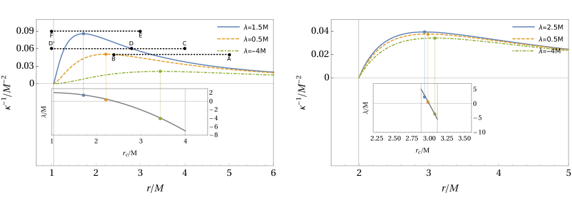
Figure 1: The $\kappa,\lambda$ as functions of $r_{c}$ in the space-time of Kerr black hole. We select spin parameter $a=0.999M$ and $a=0.1M$ in left panel and right panel, respectively.

2.2 Measurement and quantification of the shadow of black holes

The boundary of the shadow in observers’ celestial sphere are determined by the light rays from unstable circular orbits. To be specific, we can consider light rays $k,w$ and $l$ from the unstable circular orbits [71]. The $k$ and $w$ denote the light rays from the photon sphere at $r_{c,\min}$ and $r_{c,\max}$, namely

$$k = p|_{r_{c}=r_{c,\min}}~{},$$ (2.18a)

$$w = p|_{r_{c}=r_{c,\max}}~{},$$ (2.18b)

where 4-velocity $p$ is shown in Eqs. (2.14). And the expression of light ray $l$ is simply

$$l = p|_{r_{c}}~{}.$$ (2.19)

For observers located at rotation plane of a rotating black hole, the light rays $k$ and $w$ propagate within the rotation plane, since $\theta$-components of the 4-velocities $k$ and $w$ remain vanished. The appearance of the shadow can be obtained via accident angles between $l$ and $w$, $l$ and $k$, and $k$ and $w$. These angles are formulated as

$$\cos\gamma = \frac{k\cdot w}{(u\cdot k)(u\cdot w)}+1~{},$$ (2.20a)

$$\cos\alpha = \frac{k\cdot l}{(u\cdot k)(u\cdot l)}+1~{},$$ (2.20b)

$$\cos\beta = \frac{l\cdot w}{(u\cdot l)(u\cdot w)}+1~{}.$$ (2.20c)

The $\alpha$, $\beta$ and $\gamma$ depend on the light rays from photon sphere and 4-velocity of an observer $u$.

By making use of spherical trigonometric, we can express celestial coordinate $\Psi$ and $\Phi$ in terms of the $\alpha,\beta$ and $\gamma$ , i.e.

$$\Psi = \arccos\left(\sigma_{\theta}\sin\beta\sqrt{1-\left(\frac{\cos\alpha-\cos\beta\cos\gamma}{\sin\beta\sin\gamma}\right)^{2}}\right)~{},$$ (2.21a)

$$\Phi = \gamma-\arccos\left(\frac{\cos\beta}{\sin\Psi}\right)~{}.$$ (2.21b)

Therefore, one can sketch the appearance of the shadow via the curve $(\Phi(r_{c}),\Psi(r_{c}))$ in observers’ celestial sphere.

However,  merely the sketch of the shadow is not enough. In order to quantify the shape of the shadow, different distortion parameters have been introduced [81, 56, 82, 83, 58]. Here, by making use of the angles in Eqs. (2.20), we can define a distortion parameter $\cos\Xi$ in the form of [72],

$$\cos\Xi \equiv \frac{1+\cos\gamma-\cos\alpha-\cos\beta}{2\sigma_{\theta}\sqrt{(1-\cos\alpha)(1-\cos\beta)}}~{},$$ (2.22)

For $\cos\Xi\equiv 0$, the shape of the shadow is circular. And the previous study [72] suggests that the $\cos\Xi\neq 0$ indicates the distortion of the shape of the shadow from circularity. The schematic diagram is shown in Figure 2. The angle $\Xi$ is defined as

$$\Xi\equiv\angle\rm{ACB}=\angle B\bar{C}D~{}.$$ (2.23)

However, we will show in section 3.2.2 that it is not true in a general case. We can further find that $\cos\Xi=\rm{const.}$ also indicates shape of the shadow being circular.

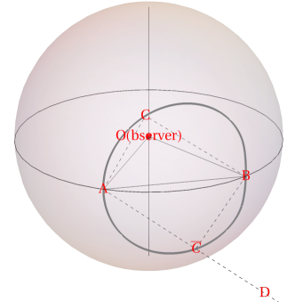
Figure 2: Schematic diagram of the distortion parameter $\cos\Xi$ in observers celestial sphere.

Rearranging Eqs. (2.21) and (2.22), we obtain equation in celestial coordinate $(\Phi,\Psi)$ for the boundary of the black hole shadow, namely,

$$0 = (1+\cos\gamma-\sin\Psi\cos\Phi-\sin\Psi\cos(\gamma-\Phi))^{2}$$ (2.24)

$$-4\cos^{2}\Xi(1-\sin\Psi\cos\Phi)(1-\sin\Psi\cos(\gamma-\Phi))~{}.$$

Here the $\gamma$ has no relevance with $\Phi$ and $\Psi$, while the $\Xi$ depends on the $\Phi$ or $\Psi$. The information about the appearance of black hole shadow is included in the $\gamma$ and distortion parameter $\cos\Xi$. The $\gamma$ describes characteristic size of the shadow, and the angle $\Xi$ describes the shape of the shadow. Therefore, in the following, we would focus on the quantities $\Xi$ and $\gamma$ influenced by inclination and motion of observers.

Besides, for the sake of intuitive, the shadow can be also sketched in a 2D-projection plane. Namely, one can transform the celestial spherical coordinates into [71],

$$Y \equiv \frac{2\sin\Phi\sin\Psi}{1+\cos\Phi\sin\Psi}~{},$$ (2.25a)

$$Z \equiv \frac{2\cos\Psi}{1+\cos\Phi\sin\Psi}~{}.$$ (2.25b)

3 Influence of inclination and motion of observers on black hole shadow

It might be the most interesting case that the black hole shadow are in the view of the observers located at rotation plane of a rotating black hole. And in this case, the shape of the shadow get the most distorted. However, it is usually not a realistic situation. The influence of inclination of black hole on the shadow also deserves to be studied [9, 53, 54, 48, 55, 56, 57, 10, 58, 59, 60, 47, 16, 61, 62]. We will further show that it is non-trivial, especially for the shadow in the view of observers at finite distance. For illustration, we consider Kerr black hole for example.

First, we consider black hole shadow in the view of static observers for different inclination of rotating black hole. Next, we will turn to the situation of geodesic observers with different velocities. For observers moving along the direction of changing $\theta$, the appearance of the shadow shows to be very interesting.

3.1 Static observers

The 4-velocities of static observers take the form of

$$u_{\rm{stc}} \equiv \frac{1}{N}\partial_{t}~{}.$$ (3.1)

In Figure 3, we present the angular diameter $\gamma$ as function of inclination $\theta$. As shown in the right panel of Figure 3, the characteristic size of the shadow $\gamma$ decreases with the inclination $\theta$ for distant observers. In contrast, in the case that observers are close to the black hole, the $\gamma$ tends to increase with the inclination, which is shown in the left panel of Figure 3. For the latter case, it is partly because the shape of the shadow is less distorted for observers at $r\rightarrow r_{c,+}$ [71].

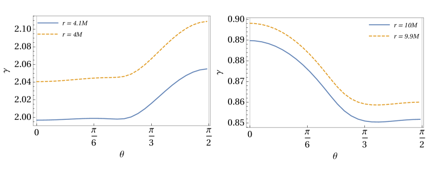
Figure 3: Characteristic size of the shadow $\gamma$ as function of inclination $\theta$ for selected distance $r$. Here, the spin parameter $a$ is set to be $0.999M$.

In Figure 4, we show how to find the transition distance ($r_{\rm t}$) between the increase trend and decrease trend presented in Figure 3. Namely, the transition distance $r_{\rm t}$ is defined with a distance that the maximums of increase trend curves and maximums of decrease trend curves are close in value. In right panel of Figure 4, we present the transition distance $r_{\rm t}$ as function of spin of black hole. It shows that the transition distance decreases with spin of black holes. For spherical black holes, the $r_{\rm t}$ tends to spatial infinity, while for extreme rotating Kerr black hole, the $r_{\rm t}$ tends to the photon sphere.

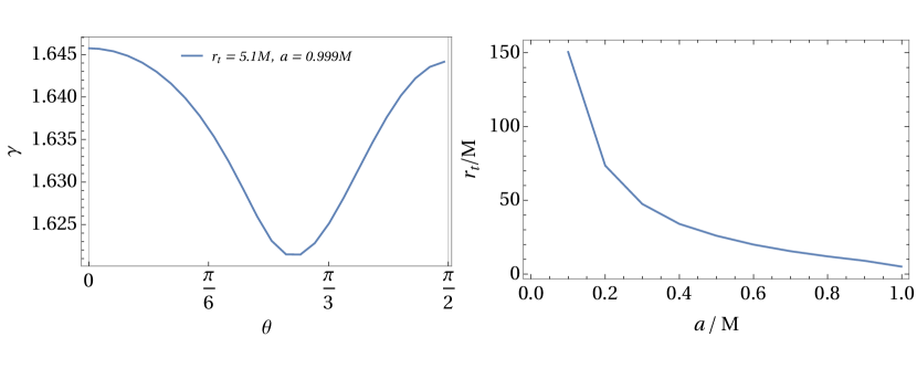
Figure 4: Left panel: Characteristic size of the shadow $\gamma$ as function of inclination $\theta$ for the transition distance $r_{\rm{t}}$. Right panel: Transition distance $r_{\rm{t}}$ as function of spin parameter $a$.

This conclusion also is showed in Figure 5 and 6, where we present the distortion parameter $\cos\Xi$ and appearance of the shadow for selected inclination $\theta$. Besides, it is nothing surprising that the shape of the shadow tends to be circular for the observers approaching the rotation axis of the black hole.

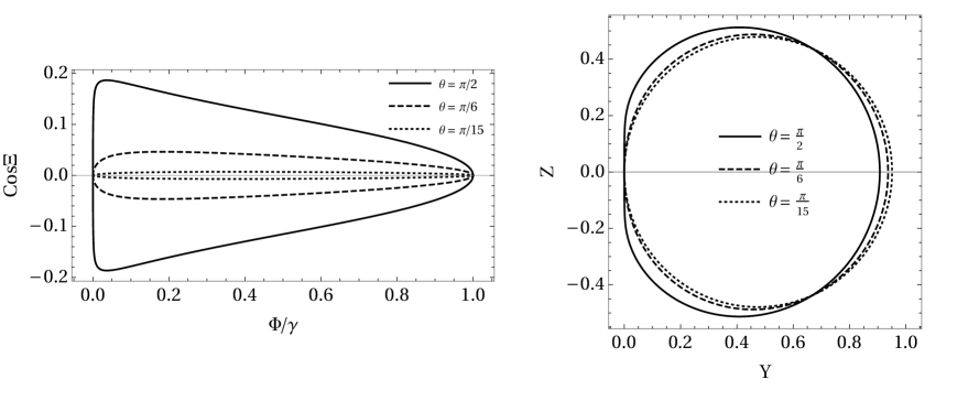
Figure 5: Left panel: distortion parameter $\cos\Xi$ as function of $\Phi/\gamma$ for different inclination $\theta$. Right panel: the appearance of the shadow in projection plane for different inclination. Here, we let observers’ position $r=10M$.

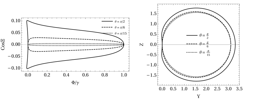
Figure 6: Left panel: distortion parameter $\cos\Xi$ as function of $\Phi/\gamma$ for different inclination $\theta$. Right panel: the appearance of the shadow in projection plane for different inclination. Here, we set observers’ position $r=4.1M$.

In Figure 7, it shows the maximum value of the distortion parameters as function of inclination for selected distance $r$. It is consistent with the previous studies [71, 72] that the distortion of the shadow get larger with the distance of the observers from the black hole. The distortion parameter is sensitive to the cases that observers are close to the black hole, namely $r\rightarrow r_{c,+}$.

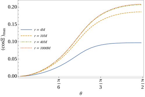
Figure 7: Maximum value of distortion parameter $\cos\Xi$ as function of inclination $\theta$.

3.2 Moving observers

In this part, we consider the cases that observers move along three representative directions. Namely, they undergo geodesic motion along the direction of changing $r$, ${\phi}$ and ${\theta}$ in Boyer-Lindquist coordinate. The schematic diagram is shown in Figure 8. For illustration, we would call these moving observers as $r$-observers, $\theta$-observers and $\phi$-observers in the following.

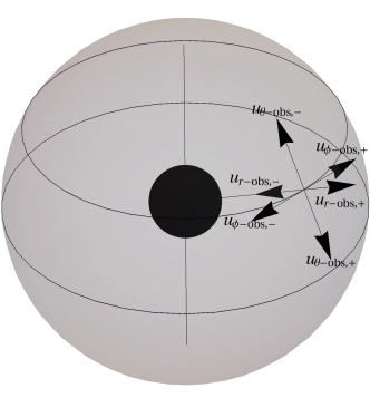
Figure 8: Schematic diagram for geodesic observers along the direction of increasing or decreasing $r$, ${\phi}$ and ${\theta}$ Boyer-Lindquist coordinate. For illustration, the 4-velocities are labelled with $r$-obs, $\theta$-obs and $\phi$-obs.

The geodesic observers are the most natural observers in the present of gravity. From Eq. (2.14) with $\epsilon=-1$, we have 4-velocities of the observers in the form of

$$u^{t} = \mathcal{E}\left(\frac{1}{N^{2}}-\frac{A}{G_{\phi}^{2}}(A+\mathcal{L})\right)~{},$$ (3.2a)

$$u^{r} = \pm\mathcal{E}\frac{\sqrt{\Delta_{r}}}{B^{2}}\sqrt{f_{1}(r;\mathcal{L})-\mathcal{K}-\left(\frac{B_{r}}{E}\right)^{2}}~{},$$ (3.2b)

$$u^{\theta} = \pm\mathcal{E}\frac{\sqrt{\Delta_{\theta}}}{B^{2}}\sqrt{\kappa+f_{2}(\theta;\mathcal{L})-\left(\frac{B_{\theta}}{E}\right)^{2}}~{},$$ (3.2c)

$$u^{\phi} = \frac{\mathcal{E}}{G_{\phi}^{2}}(A+\mathcal{L})~{}.$$ (3.2d)

In order to distinguish above 4-velocities with that of light rays, we have substituted the integral constant $E,\lambda$ and $\kappa$ in Eqs. (2.14) into $\mathcal{E},\mathcal{L}$ and $\mathcal{K}$ in Eqs. (3.2), respectively. The trajectories of the geodesic observers are not limited to circular orbits. It should be distinguished with the geodesic observers in previous studies of black hole shadow [72].

For $r$-observers, they are instantaneously along the direction of $r$, i.e. $u^{\theta}=u^{\phi}=0$. Thus, we can rewrite the velocities by fixing the constant constant $\mathcal{L}$ and $\mathcal{K}$,

$$u_{r\text{-}\rm{obs,\pm}} = \frac{\mathcal{E}}{N^{2}}\partial_{t}\pm\frac{1}{B}\sqrt{\Delta_{r}\left(\left(\frac{\mathcal{E}}{N}\right)^{2}-1\right)}\partial_{r}~{}.$$ (3.3)

Similar, for $\theta$-observers, we have

$$u_{\theta\text{-obs},\pm} = \frac{\mathcal{E}}{N^{2}}\partial_{t}\pm\frac{\sqrt{\Delta_{\theta}}}{B}\sqrt{\left(\frac{\mathcal{E}}{N}\right)^{2}-1}\partial_{\theta}~{}.$$ (3.4)

And the 4-velocities of $\phi$-observers are

$$u_{\phi\text{-}\rm{obs,\pm}} = \left(\frac{\mathcal{E}}{N^{2}}\mp\frac{A}{G_{\phi}}\sqrt{\left(\frac{\mathcal{E}}{N}\right)^{2}-1}\right)\partial_{t}\pm\left(\frac{1}{G_{\phi}}\sqrt{\left(\frac{\mathcal{E}}{N}\right)^{2}-1}\right)\partial_{\phi}~{}.$$ (3.5)

The integral constant $\mathcal{E}$ is the only one left in Eq. (3.3)–(3.5). In the case of $\mathcal{E}=N$, above velocities describe static observers. In order to compare the shadow influenced by observers moving in different directions, we have to introduce speed of these velocities. To be specific, we consider the relative speed with respect to static observers [84],

$$\upsilon=\frac{|\gamma^{*}u|}{\sqrt{u_{\rm{stc}}\cdot u}}=\sqrt{1-\left(\frac{N}{\mathcal{E}}\right)^{2}}~{},$$ (3.6)

where the $\gamma^{*}$ is the projection operator with respect to the static observers, i.e., $\gamma^{\mu}_{\nu}=u_{\rm{stc}}^{\mu}u_{\rm{stc},\nu}+\delta^{\mu}_{\nu}$. The second equal sign shows that the 3-velocities are determined by the integral constant $\mathcal{E}$ and the location of observers. The definition of the 3-speed might not be physical, because the coordinate speed might not be measured directly in principle. Here, we simply wish to make sense of different choice of $\mathcal{E}$. We are not tended to present a well-defined 3-speed in curved space-time.

3.2.1 r-observers and $\phi$-observers

In Figure 9, we present the distortion parameter and appearance of the shadow for selected inclinations $\theta$ in the view of $r$-observers. And in Figure 10, we present the distortion parameter and appearance of the shadow for selected inclination $\theta$ in the view of $\phi$-observers. The shape of the shadow tends to be circular with $\theta\rightarrow 0$. In Figure 11, we compare the distortion parameters $\cos\Xi$ and appearance of the shadows among $r$-observers and $\phi$-observes. Without the distortion parameter, it seems difficult to tell the difference of the shape of the shadow by eyes. As shown in the right panel of Figure 11, the size of the shadow increases with $r$-components of the 4-velocities of $r$-observers, while it decreases with $\phi$-components of the 4-velocities of $\phi$-observers.

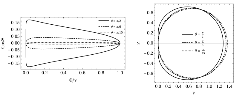
Figure 9: Left panel: distortion parameter $\cos\Xi$ as function of $\Phi/\gamma$ for different inclination $\theta$. Right panel: the appearance of the shadow in projection plane for different inclination. Here, we set $r$-observers $u_{r\text{-}\rm{obs},+}$ at $r=10M$ and $\upsilon=0.3$.

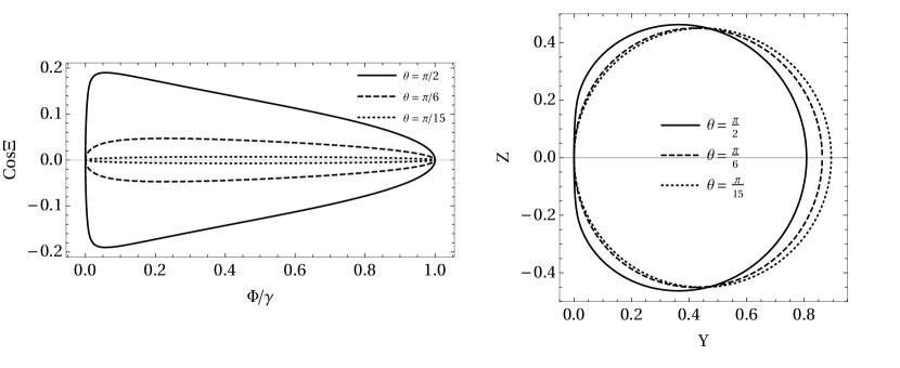
Figure 10: Left panel: distortion parameter $\cos\Xi$ as function of $\Phi/\gamma$ for different inclination $\theta$. Right panel: the appearance of the shadow in projection plane for different inclination. Here, we set $\phi$-observers $u_{\phi\text{-}\rm{obs},+}$ at $r=10M$ and $\upsilon=0.3$.

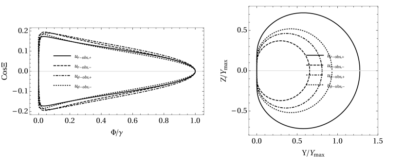
Figure 11: Left panel: distortion parameter $\cos\Xi$ as function of $\Phi/\gamma$ for different observes. Right panel: the appearance of the shadow in projection plane for different inclination. Here, we set observers at $r=10M$, $\theta=\frac{\pi}{2}$ and $\upsilon=0.3$.

In Figure 12, we show the characteristic size $\gamma$ as function of inclination $\theta$ for selected observers at a fixing distance. It is similar to that of static observers. For observers at different distance, there is contrast tendency of characteristic size $\gamma$ changing with inclination $\theta$.

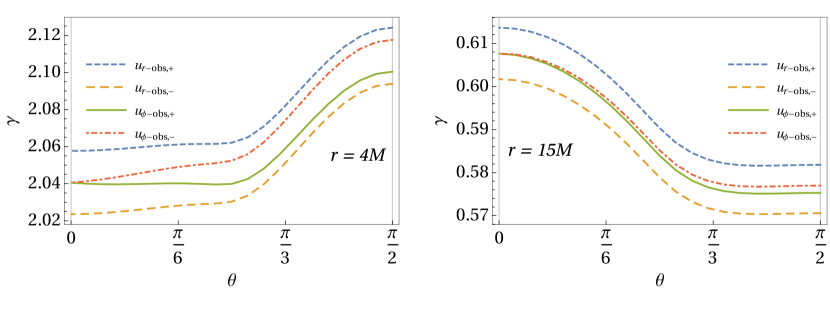
Figure 12: characteristic size $\gamma$ as function of inclination $\theta$ for different observers at the same speed $\upsilon=0.01$. The observes shown in the left panel are close to the black hole at $r=4M$, while the right panel describe the $\gamma$ with respect to more distant observers $r=15M$.

3.2.2 $\theta$-observers

For $r$-observers and $\phi$-observers, the influences of inclination is little different from that of the static observers. However, there would be something new on the shadow in the view of the $\theta$-observers. In left panel of Figure 13, we present the distortion parameter $\cos\Xi$ as function of $\Phi/\gamma$. It was expected that the shape of the shadow tends to be circular for the observers at inclination $\theta=0^{\circ}$. However, the distortion parameters $\Xi$ does not tends to $\pi/2$ as inclination $\theta\rightarrow 0^{\circ}$. In order to make it more clear, we present the appearance of the shadow in the projection plane in right panel Figure 13. We also present the plots in Figure 14 for a smaller spin parameter. The shapes of the shadow are similar to those in the view of static observers. However, apparent difference is that the shadow seems to be rotated by a specific angle in the projection plane.

Here, we should clarify whether it is caused by the way that we calculate black hole shadow. In the case of observers located at rotation plane of a rotating black hole, we have known it clearly that the light rays $k$ and $w$ exactly propagates within the rotation plane [71]. These reference light rays $k$ and $w$ should mark the fundamental plane in observers’ celestial sphere. One can confirm that the point A and B in fundamental plane shown in Figure 2 always corresponds to the rotation plane of the black hole. Therefore, the rotated image of the shadow shown in the right panel of Figure 13 must be a physical result caused by the motion of observers. The ways of the shadow getting distorted depend not only on the spin of the black hole, but also the velocities of observers.

We quantify the rotation angle via the distortion parameter $\Xi$, which is

$$\Sigma\equiv\frac{\pi}{2}-\Xi|_{\theta=0}~{}.$$ (3.7)

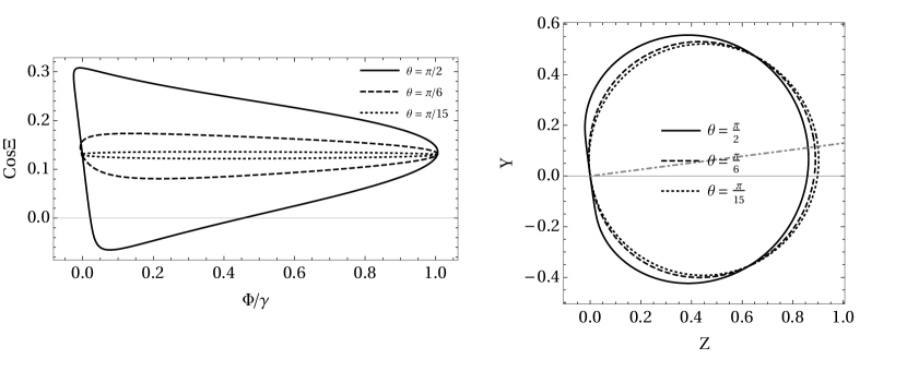
Figure 13: Left panel: distortion parameter $\cos\Xi$ as function of $\Phi/\gamma$ for different inclination $\theta$. Right panel: the appearance of the shadow in projection plane for different inclination. Here, we set $\theta$-observers’ $u_{\theta\text{-}\rm{obs},+}$ at $r=10M$, $\upsilon=0.3$ and spin parameter $a=0.999M$. The angle $\Sigma$ is shown in dot-dashed line.

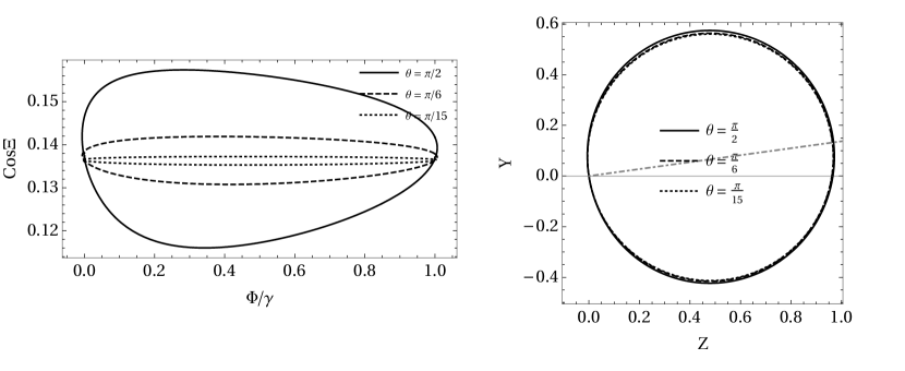
Figure 14: Left panel: distortion parameter $\cos\Xi$ as function of $\Phi/\gamma$ for different inclination $\theta$. Right panel: the appearance of the shadow in projection plane for different inclination. Here, we set $\theta$-observers’ $u_{\theta\text{-}\rm{obs},+}$ at $r=10M$, $\upsilon=0.3$, and spin parameter $a=0.6M$. The angle $\Sigma$ is shown in dot-dashed line.

In the right panel of Figure 13, we also plot the angle $\Sigma$ in dotted-dashed line. It is basically derived from the geometric property of angle $\Xi$. In Figure 15. we present the rotation angle $\Sigma$ of image as function of the distance. The angle $\Sigma$ decreases with distance of observers from the black hole. It indicates that the effect get more apparent for observers at finite distance. It could be understood that the observation for an observer in curved space-time is tended to be more non-trivial. Besides, it is also interesting to consider whether the $\Sigma$ depends on the spin of a black hole. As shown in Figure 15, the spin might have not considerable influence on the $\Sigma$. Here, we also could not excluded the possibility that the deviations for different spin (etc. $\Sigma|_{a_{1}}-\Sigma|_{a_{2}}$) are originated from the trail definition of $\Sigma$ in Eq. (3.7), and is thus un-physical.

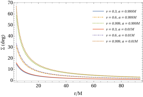
Figure 15: Rotation angle $\Sigma$ as function of coordinate $r$ of $\theta$-observers for selected speed $\upsilon$ and spin parameter $a$.

4 A formalism for velocity perturbation of distant observers

As shown in Section 3, motion of observers has influence on the appearance of black hole shadow. Besides the geodesic motion around the centre black hole, there are also influence from local orbital motions in a local gravitational potential, such as the EHT on the Earth orbits the Sun in its local gravity potential. In this section, we will turn to this local orbital motion. As these parts of velocities of observers are usually very small ($\frac{\upsilon}{c}\simeq 10^{-5}$ for the Earth’s orbit), we consider the influence of local gravitational potential via introducing expansion of velocities of observers, i.e.,

$$u^{\mu}\rightarrow u^{(0),\mu}+\delta u^{\mu}~{}.$$ (4.1)

The $t$-component of the 4-velocity is determined by normalization condition $u^{\mu}u_{\mu}=-1$ and $u^{(0),\mu}u_{\mu}^{(0)}=-1+\mathcal{O}(\delta u)$. For illustration, we would call the changes of velocity $\delta u$ in Eq. (4.1) as local velocity.

By making use of the expansion of the velocities Eq. (4.1), we can re-express the angular distances $(\alpha,\beta,\gamma)$ in Eqs. (2.20),

$$1-\cos\alpha = (1-\cos\alpha^{(0)})(1+2\delta_{\alpha})~{},$$ (4.2a)

$$1-\cos\beta = (1-\cos\beta^{(0)})(1+2\delta_{\beta})~{},$$ (4.2b)

$$1-\cos\gamma = (1-\cos\gamma^{(0)})(1+2\delta_{\gamma})~{},$$ (4.2c)

where the $\alpha^{(0)},\beta^{(0)}$ and $\gamma^{(0)}$ are the angular distances with respect to the 4-velocity $u^{(0),\mu}$, and the relative deviations of the angular distances $\delta_{\alpha}$, $\delta_{\beta}$ and $\delta_{\gamma}$ are obtained to be

$$\delta_{\alpha} = -\frac{1}{2}\left(\frac{\delta u\cdot k}{u^{(0)}\cdot k}+\frac{\delta u\cdot l}{u^{(0)}\cdot l}\right)~{},$$ (4.3a)

$$\delta_{\beta} = -\frac{1}{2}\left(\frac{\delta u\cdot l}{u^{(0)}\cdot l}+\frac{\delta u\cdot w}{u^{(0)}\cdot w}\right)~{},$$ (4.3b)

$$\delta_{\gamma} = -\frac{1}{2}\left(\frac{\delta u\cdot k}{u^{(0)}\cdot k}+\frac{\delta u\cdot w}{u^{(0)}\cdot w}\right)~{}.$$ (4.3c)

For simplicity, above equations are expressed without indices. Here, the dot product is defined as $u\cdot k\equiv g_{\mu\nu}u^{\mu}k^{\nu}$ ($\mu=0,1,2,3$). As shown in Eqs. (4.3), at the leading order, the changes of the angular distances are proportional to local velocity $\delta u^{\mu}$.

Using Eqs. (2.22) and (4.3), we can obtain the relative deviation of distortion parameter in terms of local velocity, namely,

$$1-\cos\Xi = (1-\cos\Xi^{(0)})(1+\delta_{\Xi})~{},$$ (4.4)

where

$$\delta_{\Xi} = \frac{\cos\Xi^{(0)}}{\cos\Xi^{(0)}-1}\left(\frac{2(\cos\gamma-1)\delta_{\gamma}-2(\cos\alpha-1)\delta_{\alpha}-2(\cos\beta-1)\delta_{\beta}}{1+\cos\gamma-\cos\alpha-\cos\beta}-\delta_{\alpha}-\delta_{\beta}\right)~{},$$ (4.5)

and the $\cos\Xi^{(0)}$ is distortion parameter with respect to 4-velocity $u^{(0),\mu}$. From Eq. (4.5), one might find that the relative deviation of the distortion parameter $\delta_{\Xi}$ is also proportional to local velocity of an observer.

The formulae in Eqs. (4.3) and (4.5) are not limited to the cases of distant observers. In principle, local metric perturbations should be introduced, in order to evaluate the local velocity $\delta u$ in a curved space-time background. For the first step, here we consider the local velocities of distant observers in an asymptotic flatness space-time. In this case, the $\delta u$ can be easily obtained via a local gravity potential in flat space-time background.

Besides, the appearance of the shadow can be also influenced by slightly changes of local displacement in orbits. If considering this part of contributions, one can obtain the formulae via expansion of $x^{\mu}\rightarrow x^{\mu}+\delta x^{\mu}$. We would also discuss this contribution in the end of the section.

4.1 Orbital observers

For a more specific study based on the formalism introduced above, we turn to consider observers orbiting around axes of $r$, $\theta$ and $\phi$. Namely, besides the background speed $u^{(0)}$, there are additional velocities $\delta\bm{u}$ from local orbits. For illustration, we will call them $r$-rotation-observers, $\theta$-rotation-observers and $\phi$-rotation-observers, respectively.

For an asymptotic flatness space-time and in the case of $r\gg M$, the metric is tended to be Minkowski space-time. We derive the $\delta\bm{u}$ for distant observers based on the Minkowski background. In this case, there is no ambiguous that $\delta\bm{u}$ can describe physical velocities of the observers.

First, if considering rotation axis $\bm{w}=w\hat{\bm{r}}$, the spatial part of local velocity $\delta\bm{u}$ takes the form of

$$\delta\bm{u}_{r\text{-rot-obs}} = -\frac{w\sin\varphi\sin(wt)\sin\theta}{\sqrt{1-(\cos\theta\cos\varphi-\cos(wt)\sin\theta\sin\varphi)^{2}}}\partial_{\theta}$$ (4.6)

$$+\frac{w\sin\varphi(\cos(wt)\cos\varphi\sin\theta+\cos\theta\sin\varphi)}{1-(\cos\theta\cos\varphi-\cos(wt)\sin\theta\sin\varphi)^{2}}\partial_{\phi}~{},$$

where the angle $\varphi$ is shown in left panel Figure 16. In this case, the amplitude of velocity $\delta\bm{u}$ can be expressed as

$$\upsilon\equiv\sqrt{\delta\bm{u}_{r\text{-rot-obs}}\cdot\delta\bm{u}_{r\text{-rot-obs}}}=wr\sin\varphi~{}.$$ (4.7)

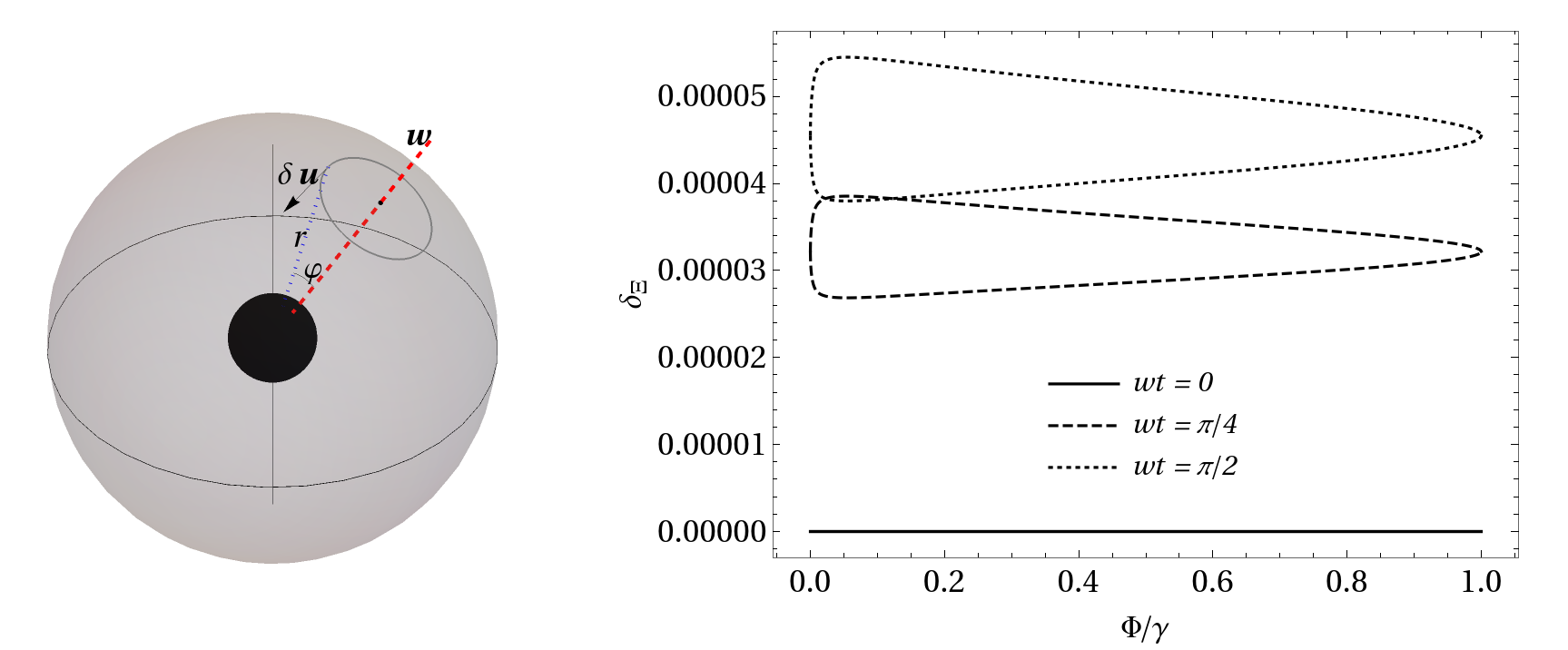
Figure 16: Left panel: schematic diagram of the orbit of the $r$-rotation-observers. Right panel: relative deviation of distortion parameter $\delta_{\Xi}$ as function of $\Phi/\gamma$. Here, we set $r=10^{3}M$ and $\theta=\frac{\pi}{3}$. And in order to present the influence of the $\delta\bm{u}$ on the shadow, we set a quite large amplitude of the speed $\upsilon=10^{-2}c$ for $r$-rotation-observers.

In right panel Figure 16, we present the relative deviation of distortion parameter $\delta_{\cos\Xi}$ as function of $\Phi/\gamma$. For a fixing orbital radius $d$ of detectors, i.e. $d\equiv r\sin\varphi$ (const.), the $\varphi$ tends to vanish as $r/M\rightarrow\infty$. In the case of $wt=0$, we have $\delta\bm{u}_{r\text{-rot-obs}}\propto\partial_{\phi}$, namely, there is no $\theta$-component of the local velocities. In contract, in the case of $wt\neq 0$, there exists $\theta$-component of local velocities. It is consistent with results shown in Section 3 that the parameter $\delta_{\Xi}$ deviated from zero is caused by observers’ motion along the direction of changing $\theta$.

Second, for rotation axis $\bm{w}=w\left(\hat{\bm{z}}\times\bm{r}\right)$ shown in Figure 17, we have spatial part of local velocity $\delta\bm{u}$ in the form of

$$\delta\bm{u}_{\phi\text{-rot-obs}} = \frac{\upsilon\sin(wt)}{\sqrt{1+\left(\frac{d}{r}\right)^{2}+\frac{2d}{r}\cos(wt)}}\partial_{r}+\frac{\upsilon}{r}\left(\frac{\frac{d}{r}+\cos(wt)}{1+\left(\frac{d}{r}\right)^{2}+\frac{2d}{r}\cos(wt)}\right)\partial_{\theta}~{},$$ (4.8)

where $d$ is orbital radius of a detector, and

$$\upsilon \equiv \sqrt{\delta\bm{u}_{\phi\text{-rot-obs}}\cdot\delta\bm{u}_{\phi\text{-rot-obs}}}=wd~{}.$$ (4.9)

In Figure 17, we present the relative deviation of distortion parameter $\delta_{\cos\Xi}$ as function of $\Phi/\gamma$ for given $wt$. The tendency of the $\delta_{\Xi}$ for $\phi$-rotation-observers is similar to that of $r$-rotation-observers. And in the case of of $wt=\pi/2$, we have $\delta\bm{u}_{\phi\text{-rot-obs}}\propto\partial_{r}$, and then the $\delta_{\Xi}$ tends to be zero.

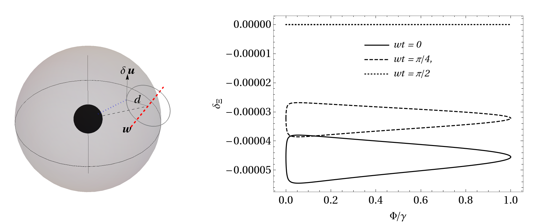
Figure 17: Left panel: schematic diagram of the orbit of the $\phi$-rotation-observers. Right panel: relative deviation of distortion parameter $\delta_{\Xi}$ as function of $\Phi/\gamma$. Here, we set $r=10^{3}M$, $\theta=\frac{\pi}{3}$ and $\upsilon=10^{-2}c$ for $\phi$-rotation-observers.

Third, for rotation axis $\bm{w}=w\left(\left(\hat{\bm{z}}\times\hat{\bm{r}}\right)\times\hat{\bm{r}}\right)$ shown in Figure 18, spatial part of local velocity $\delta\bm{u}$ is

$$\delta\bm{u}_{\theta\text{-rot-obs}} = \frac{drw\sin(wt)}{\sqrt{d^{2}+r^{2}+2dr\cos(wt)}}\partial_{r}$$ (4.10)

$$+\frac{d^{2}w\cos\theta\sin(wt)(d+{r}\cos(wt))}{(d^{2}+r^{2}+2d{r}\cos(wt))\sqrt{2dr\cos(wt)\sin\theta+r^{2}\sin^{2}\theta+d^{2}(1-\cos^{2}(wt)\cos^{2}\theta)}}\partial_{\theta}$$

$$+\frac{dw\sin\theta(d+{r}\cos(wt))}{r^{2}\sin^{2}\theta+2dr\cos(wt)\sin^{2}\theta+d^{2}(1-\cos^{2}(wt)\cos^{2}\theta)}\partial_{\phi}~{}.$$

In Figure 18, we present the relative deviation of distortion parameter $\delta_{\cos\Xi}$ as function of $\Phi/\gamma$ for given $wt$ of $\delta\bm{u}_{\theta\text{-rot-obs}}$. In this case, one can find the parameter $\delta_{\Xi}$ are much less than those of $\delta\bm{u}_{\phi\text{-rot-obs}}$ and $\delta\bm{u}_{r\text{-rot-obs}}$.

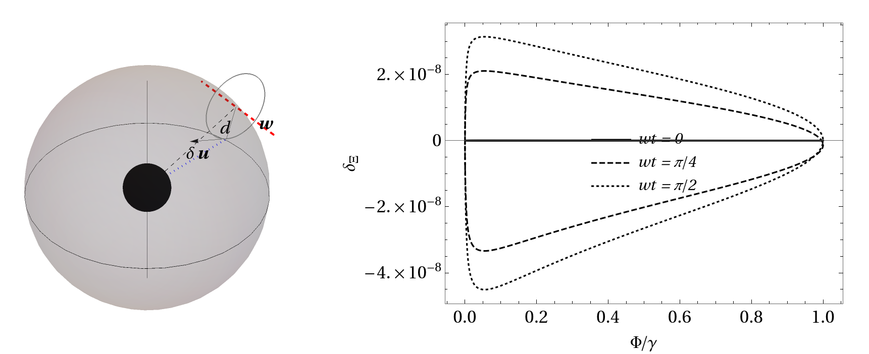
Figure 18: Left panel: schematic diagram of the orbit of the $\theta$-rotation-observers. Right panel: relative deviation of distortion parameter $\delta_{\Xi}$ as function of $\Phi/\gamma$. Here, we set $r=10^{3}M$, $\theta=\frac{\pi}{3}$ and $\upsilon=10^{-2}c$ for $\theta$-rotation-observers.

Through the $\delta_{\Xi}$ for the three representative observers, it is found that the $\theta$-component of the local velocities dominate the $\delta_{\Xi}$. As shown in Figure 13, one can no longer determine the rotation axis via the appearance of the shadow in practice. Fortunately, we might have alternative approach by making use of the quantity $\delta_{\Xi}$. Adjusting orbit of a satellite for a minimum $\delta_{\Xi}$, then one can learn that the rotation axis of black hole and the rotation axis of the orbit would turn to be coplanar in this adjusted orbit.

4.2 Earth’s orbit and Sun’s Galactic orbit

The EHT project has already aimed at the shadow of Sgr A* in the centre of Milky way [2]. In the future, lots of information about the centre black hole would be collected. Therefore, it is necessary to consider influence on the black hole shadow from physical point of view. As known that the EHT are a set of telescopes located at the Earth. The Earth orbits the Sun. And the Sun orbits the centre of the Milky way. There is local velocity of the Earth with respect to the centre of Milky way around the order of magnitude $10^{-5}c$. It seems not unpractical to consider the influence of motion of detectors or telescopes on the shadow of Sgr A*.

In section 18, we have shown that the characteristic size $\gamma$ and the distortion parameter $\cos\Xi$ are affected by the local velocities in Eqs. (4.2c) and (4.5). Besides, the Earth’s orbit also present a local displacement at the order of the orbital diameter. Thus, in this part, we will study leading order effect of both the local displacements and local velocities of detectors. In order to make these orbits more realistic, we utilize the data of Sgr A* and solar system as shown in Table 1. For illustration, we simply assume Kerr black hole with spin parameter $a\simeq 1$ as a description of Sgr A*. In principle, it is not difficult to extend the study on a more realistic black hole.

Table 1: Data of Sgr A* and solar system [85, 86]

Mass of Sgr A* ($M$)	$4\times 10^{6}M_{\odot}$	$M$
Sun’s distance to galactic centre ($R_{\odot}$)	$8\rm{kpc}$	$4.18\times 10^{10}\frac{GM}{c^{2}}$
Galactic years ($T_{\odot}$)	$225\rm{Myr}$	$3.60\times 10^{14}\frac{GM}{c^{3}}$
Earth’s distance to sun ($d_{\oplus}$)	$1\rm{au}$	$25.3\frac{GM}{c^{2}}$
Earth’s orbital angular velocities to sun $(w_{\oplus})$	$w_{0}=\frac{2\pi}{1\rm{yr}}$, $l=94.6^{\circ}$, $b=29.8^{\circ}$	$w_{0}=3.93\times 10^{-6}\frac{c^{3}}{GM}$

For two light rays from the photon sphere, angle $\psi$ between two incident light rays in of observer’s celestial sphere is

$$\cos\psi = \frac{p_{1}\cdot p_{2}}{(u\cdot p_{1})(u\cdot p_{2})}+1~{},$$ (4.11)

where $p_{i}\equiv p|_{r_{c}=r_{c,i}}$ and $u$ is 4-velocity of the Sun with respect to the central of the Milky way. The angular distance $\psi$ could be $\alpha$, $\beta$ or $\gamma$. We expand the angle $\psi$ at $r/M\rightarrow\infty$, namely

$$\cos\psi = 1-\frac{\mathcal{C}_{\psi}^{(1)}}{r^{2}}-\frac{\mathcal{C}^{(2)}_{\psi}}{r^{3}}-\frac{\mathcal{C}_{\psi}^{(3)}}{r^{4}}+\mathcal{O}\left(\left(\frac{M}{r}\right)^{4}\right)~{},$$ (4.12)

where

$$\mathcal{C}_{\psi}^{(1)} \equiv \frac{\frac{\kappa_{1}+\kappa_{2}}{2}-(\lambda_{1}-a)(\lambda_{2}-a)-\sqrt{\kappa_{1}-(a-\lambda_{1})^{2}}\sqrt{\kappa_{2}-(a-\lambda_{2})^{2}}}{\mathcal{E}^{2}}~{},$$ (4.13a)

$$\mathcal{C}_{\psi}^{(2)} \equiv \left((\lambda_{1}+\lambda_{2})\sqrt{1-\frac{1}{\mathcal{E}^{2}}}-4M\right)\mathcal{C}_{\psi}~{},$$ (4.13b)

$$\mathcal{C}_{\psi}^{(3)} \equiv \frac{1}{\mathcal{E}^{2}}\left(\frac{1}{8}(\kappa_{1}-\kappa_{2})(\kappa_{1}-\kappa_{2}+4a(\lambda_{1}-\lambda_{2}))\right)$$ (4.13c)

$$+\frac{\mathcal{C}_{\alpha}}{\sqrt{\mathcal{E}^{2}-1}}\Big{(}4\mathcal{E}M\left(a(\mathcal{E}^{2}-1)+M\mathcal{E}\sqrt{\mathcal{E}^{2}-1}\right)$$

$$+(\mathcal{E}^{2}-1)^{\frac{3}{2}}(\lambda_{1}^{2}+\lambda_{2}^{2}+\lambda_{1}\lambda_{2})+\mathcal{E}(6-5\mathcal{E}^{2})M(\lambda_{1}+\lambda_{2})\Big{)}~{}.$$

In above expressions, we have let $\lambda_{i}\equiv\lambda|_{r_{c}=r_{c,i}}$, and $\kappa_{i}\equiv\kappa|_{r_{c}=r_{c,i}}$. The $\lambda$ and $\kappa$ are functions of $r_{c}$  shown in Eqs. (2.16). By making use of Eq. (4.12), we obtain the leading order of relative deviation of the $\psi$ caused by local displacement $\Delta r$, i.e.

$$\delta_{\psi,\rm{disp}}\equiv\frac{\Delta\psi}{\psi} = -\frac{\Delta r}{r}+\mathcal{O}\left(\left(\frac{M}{r}\right)^{2}\right)~{},$$ (4.14)

This quantity have no relevance with coefficient $\mathcal{C}^{(i)}_{\psi}$. Considering the shadow of Sgr A* observed by the EHT, we can let $\Delta r\simeq 2d_{\oplus}$ and $r\simeq r_{\odot}$.

Therefore, we can re-express the $\psi$ in the expansion both including the contributions from local velocity and displacement,

$$\psi = \psi^{(0)}(1+\delta_{\psi,\rm{velo}}+\delta_{\psi,\rm{disp}})~{},$$ (4.15)

where the expression of $\delta_{\psi,\rm{velo}}$ is similar to that of $\delta_{\alpha}$, $\delta_{\beta}$ and $\delta_{\gamma}$, i.e.

$$\delta_{\psi,\rm{velo}}=-\frac{1}{2}\left(\frac{\delta u\cdot p_{1}}{u^{(0)}\cdot p_{2}}+\frac{\delta u\cdot p_{2}}{u^{(0)}\cdot p_{2}}\right)~{},$$ (4.16)

In order to compare the relative deviation of local velocities $\delta_{\psi,\rm{velo}}$ with the $\delta_{\psi,\rm{disp}}$, we expand the $\delta_{\psi,\rm{velo}}$ in Eq. (4.16) in terms of $r/M\rightarrow\infty$,

$$\delta_{\psi,\rm{velo}} = \delta_{\psi,\rm{velo}}^{(0)}+\frac{1}{r}\delta^{(1)}_{\psi,\rm{velo}}+\mathcal{O}\left(\left(\frac{M}{r}\right)^{2}\right)~{},$$ (4.17)

where

$$\delta^{(0)}_{\psi,\rm{velo}} \equiv \frac{1}{\mathcal{E}}(\delta u^{r}-\delta u^{0})~{},$$ (4.18)

$$\delta^{(1)}_{\psi,\rm{velo}} \equiv \frac{1}{2\mathcal{E}}\Bigg{(}4M\delta u^{0}+\upsilon_{\theta}\left(\sqrt{\kappa_{1}-(\lambda_{1}-a)^{2}}+\sqrt{\kappa_{2}-(\lambda_{2}-a)^{2}}\right)$$ (4.19)

$$+(\lambda_{1}+\lambda_{2})\left(\sqrt{1-\frac{1}{\mathcal{E}^{2}}}(\delta u^{r}-\delta u^{0})+\upsilon_{\phi}\right)\Bigg{)}~{}.$$

As shown in Section 3, it is found that $\delta u^{t},\delta u^{r}\simeq\mathcal{O}(1)$ and $\delta u^{\theta}$, $\delta u^{\phi}\simeq\mathcal{O}\left(\frac{1}{r}\right)$ for distant observers. Therefore, in Eq. (4.17), we have parametrized the local velocity as

$$\delta u^{\mu} = \left(\delta u^{t},\delta u^{r},\frac{\upsilon_{\theta}}{r},\frac{\upsilon_{\phi}}{\rm{rsin}\theta}\right)~{}.$$ (4.20)

And the Eq. (4.17) can be re-expressed as

$$\psi = \psi^{(0)}\left(1+\frac{\delta u^{r}-\delta u^{0}}{\mathcal{E}}+\frac{\delta^{(1)}_{\psi,\rm{velo}}-\Delta r}{r}+\mathcal{O}\left(\left(\frac{M}{r}\right)^{2},\delta u\right)\right)~{}.$$ (4.21)

The leading order term of deviation of $\psi$ is dominated by the local velocities $\delta u^{\mu}$ and $\Delta r/r$. It has no relevance with information of the black hole. Using the data in Table 1, we compare different contributions of the deviation of $\psi$ in order of magnitude, which is shown in Table 2.

For the shape of the black hole shadow, we also expand the deviation of distortion parameter $\cos\Xi$ in terms of $r/M\rightarrow\infty$ and $\delta u$, namely,

$$1-\cos\Xi = (1-\cos\Xi^{(0)})(1+\delta_{\Xi}+\delta_{\Xi,\rm{disp}})~{},$$ (4.22)

where

$$\delta_{\Xi,\rm{disp}} \equiv -\frac{2\Delta r}{r^{3}}\frac{1}{\mathcal{C}_{\alpha}^{(1)}+\mathcal{C}_{\beta}^{(1)}-\mathcal{C}_{\gamma}^{(1)}-2\sigma\sqrt{\mathcal{C}_{\alpha}^{(1)}\mathcal{C}_{\beta}^{(1)}}}\Bigg{(}\mathcal{C}_{\alpha}^{(3)}+\mathcal{C}_{\beta}^{(3)}-\mathcal{C}_{\gamma}^{(3)}$$ (4.23)

$$-(\mathcal{C}_{\alpha}^{(2)}+\mathcal{C}_{\beta}^{(2)}-\mathcal{C}_{\gamma}^{(2)})\left(\frac{\mathcal{C}_{\alpha}^{(2)}}{2\mathcal{C}_{\alpha}^{(1)}}+\frac{\mathcal{C}_{\beta}^{(2)}}{2\mathcal{C}_{\beta}^{(1)}}\right)$$

$$+\left(\mathcal{C}_{\alpha}^{(1)}+\mathcal{C}_{\beta}^{(1)}-\mathcal{C}_{\gamma}^{(1)}\right)\left(\frac{3}{4}\left(\frac{\mathcal{C}_{\alpha}^{(2)}}{\mathcal{C}_{\alpha}^{(1)}}\right)^{2}+\frac{3}{4}\left(\frac{\mathcal{C}_{\beta}^{(2)}}{\mathcal{C}_{\beta}^{(1)}}\right)^{2}+\frac{\mathcal{C}_{\alpha}^{(2)}\mathcal{C}_{\beta}^{(2)}}{2\mathcal{C}_{\alpha}^{(1)}\mathcal{C}_{\beta}^{(1)}}-\frac{\mathcal{C}_{\alpha}^{(3)}}{\mathcal{C}_{\alpha}^{(1)}}-\frac{\mathcal{C}_{\beta}^{(3)}}{\mathcal{C}_{\beta}^{(1)}}\right)\Biggl{)}$$

$$+\mathcal{O}\left(\left(\frac{M}{r}\right)^{4}\right)~{},$$

and we also expand expression of $\delta_{\Xi}$ in Eq. (4.5) at $r/M\rightarrow\infty$

$$\delta_{\Xi} = \frac{1}{r}\left(\frac{-2\mathcal{C}_{\gamma}^{(1)}\delta_{\gamma,\rm{velo}}^{(1)}+(\mathcal{C}_{\alpha}^{(1)}-\mathcal{C}_{\beta}^{(1)}+\mathcal{C}_{\gamma}^{(1)})\delta_{\alpha,\rm{velo}}^{(1)}+(\mathcal{C}_{\beta}^{(1)}-\mathcal{C}_{\alpha}^{(1)}+\mathcal{C}_{\gamma}^{(1)})\delta_{\beta,\rm{velo}}^{(1)}}{2\sqrt{\mathcal{C}_{\alpha}^{(1)}\mathcal{C}_{\beta}^{(1)}}}\right)$$ (4.24)

$$+\mathcal{O}\left(\left(\frac{M}{r}\right)^{2}\right)~{}.$$

The $\delta_{\gamma,\rm{velo}}^{(1)}$, $\delta_{\alpha,\rm{velo}}^{(1)}$ and $\delta_{\beta,\rm{velo}}^{(1)}$ are relative deviations of angular distances defined in Eqs. (4.3). For distant observers, we have $\delta_{\Xi}\simeq\delta u/r$ and $\delta_{\Xi,\rm{disp}}\simeq\Delta r/r^{3}$. It suggests that the deviation of distortion parameter $\delta_{\Xi}\gg\delta_{\Xi,\rm{disp}}$. Namely, local velocity $\delta u$ has more significant influence on the shape of the shadow than the local displacement $\Delta r$. In Table 2, we present order of magnitude estimation for the shape of the shadow of Sgr A*.

Table 2: Order of magnitude of relative deviation of $\delta_{\gamma}$ and $\delta_{\Xi}$ for the shadow of Sgr A*

Relative deviation		Estimators	Order of magnitude
$\delta_{\gamma}$	$|\delta_{\gamma,\rm{velo}}|_{\max}$	$\delta u/c$	$10^{-4}$
	$\delta_{\gamma,\rm{disp}}$	$\frac{2d_{\oplus}}{r}$	$10^{-10}$
$\delta_{\Xi}$	$|\delta_{\Xi}|_{\max}$	$\frac{\delta u}{r}/\frac{GM}{c^{3}}$	$10^{-14}$
	$|\delta_{\Xi,\rm{disp}}|_{\max}$	$\frac{2d_{\oplus}}{r^{3}_{\odot}}/\left(\frac{c^{2}}{GM}\right)^{2}$	$10^{-30}$

For the supermassive black hole Sgr A*, it is found that the local velocities of observers dominate the effect on the size and shape of the black hole shadow. Besides, we also present $\delta_{\Xi}$ and $\delta_{\Xi,\rm{disp}}$ as functions of $r_{c}$ in Figure 19. It shows that the local velocities and the local displacements have influence on the distortion parameter $\Xi$ in a different way.

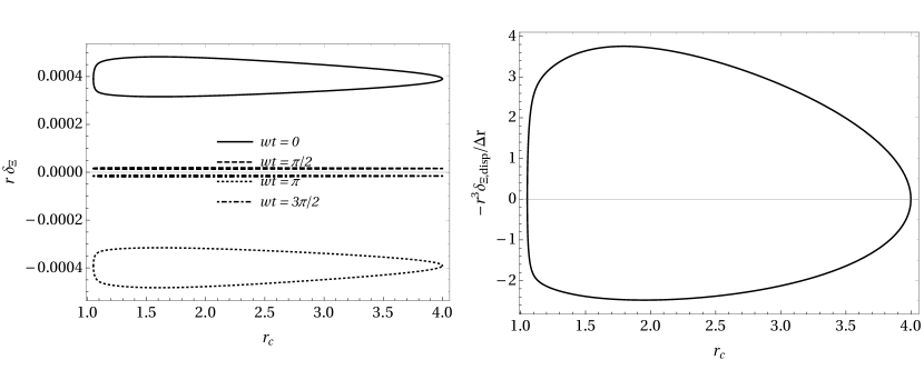
Figure 19: Left panel: deviation of distortion parameter of Earth’s orbit $\delta_{\Xi}$ as function of $r_{c}$. Right panel: deviation of distortion parameter $\delta_{\Xi,\rm{disp}}$ of Earth’s orbit as function of $r_{c}$. The 4-velocity describing the motion of the Earth is obtained by making use of the data of Sgr A* and solar system in Table 1

5 Conclusions and discussions

In this paper, we investigated influence of Earth’s orbit on the shadow of Sgr A*. We extended the previous studies [71, 72] to arbitrary inclination, and observers at different velocities. It was partly motivated by the inclination of the Earth’s orbit are not located at galactic plane [86]. In this study, it was found that the appearance of the shadow would be rotated by a certain angle for an observer moving towards direction of changes of inclination $\theta$. It is beyond pioneer’s study [20] that distorted shape of the shadow suggests spin direction of a rotating black hole. In order to handle local orbits of observers with respect to the black hole Sgr A*, we presented a formalism for calculating the shadow in terms of the local velocity expansion. It showed that the influence of the orbital velocity of the Earth on the shadows is much larger than that of displacement in Earth’s orbit. For the shadow of the Sgr A*, we obtained the deviation of characteristic size $\delta_{\gamma}$ of the shadow around $10^{-4}$. And the deviation of the distortion parameter $\delta_{\Xi}$ of the shadow is around $10^{-14}$.

It is found that rotation axis of a rotating black hole might not be extracted from its shadow. The ways of the shadow getting distorted depend not only on the spin of the black hole, but also the velocities of observers. This effect is shown to be less important for an observer at spatial infinity in an asymptotic flatness space-time. Perhaps, it might suggest that the observation for an observer in curved space-time is tended to be more non-trivial.

In the present approach for calculating the black hole shadow, the reference light rays $k$ and $w$ are chosen to be the 4-velocities with vanished $\theta$-components for observers with $\theta=\pi/2$. It is still possible to define reference light rays based on appearance of the shadow. Namely, one can let the reference rays locate the minimum diameter of the shadow in observers’ celestial sphere. This scheme might be more practical for extracting information of a black hole from its shadow, although it could be rather artificial in formulae.

Besides, as it shown in right panel of Figure 13, the shape of the shadow is seems to be unchanged. It might indicate that shape of the shadow from magnitude of spin is intrinsic prosperity of a rotating black hole. In succeeding studies, a more rigid study on this issue should be given.

References

- [1] Event Horizon Telescope collaboration, First M87 Event Horizon Telescope Results. I. The Shadow of the Supermassive Black Hole, The Astrophysical Journal Letters 875 (2019) L1 [1906.11238].
- [2] Event Horizon Telescope collaboration, First M87 Event Horizon Telescope Results. IV. Imaging the Central Supermassive Black Hole, The Astrophysical Journal Letters 875 (2019) L4 [1906.11241].
- [3] J. W. Moffat, Black holes in modified gravity (MOG), European Physical Journal C 75 (2015) 175.
- [4] J. W. Moffat, Modified gravity black holes and their observable shadows, European Physical Journal C 75 (2015) 130.
- [5] J. W. Moffat and V. T. Toth, The masses and shadows of the black holes Sagittarius A* and M87* in modified gravity (MOG), Physical Review D 101 (2020) 024014.
- [6] R. Kumar and S. G. Ghosh, Black Hole Parameter Estimation from Its Shadow, The Astrophysical Journal 892 (2020) 78.
- [7] K. Jusufi, M. Jamil, H. Chakrabarty, Q. Wu, C. Bambi and A. Wang, Rotating regular black holes in conformal massive gravity, Physical Review D 101 (2020) 044035.
- [8] T. Zhu, Q. Wu, M. Jamil and K. Jusufi, Shadows and deflection angle of charged and slowly rotating black holes in Einstein-AEther theory, Physical Review D 100 (2019) 044055.
- [9] S. X. Tian and Z.-H. Zhu, Testing the Schwarzschild metric in a strong field region with the Event Horizon Telescope, Physical Review D 100 (2019) 064011.
- [10] A. Övgün, İ. Sakallı and J. Saavedra, Shadow cast and Deflection angle of Kerr-Newman-Kasuya spacetime, Journal of Cosmology and Astroparticle Physics 2018 (2018) 041.
- [11] R. A. Hennigar, M. B. J. Poshteh and R. B. Mann, Shadows, signals, and stability in Einsteinian cubic gravity, Physical Review D 97 (2018) 064041.
- [12] D. Ayzenberg and N. Yunes, Black hole shadow as a test of general relativity: quadratic gravity, Classical and Quantum Gravity 35 (2018) 235002.
- [13] R. Konoplya, L. Rezzolla and A. Zhidenko, General parametrization of axisymmetric black holes in metric theories of gravity, Physical Review D 93 (2016) 064015.
- [14] Z. Li and C. Bambi, Measuring the Kerr spin parameter of regular black holes from their shadow, Journal of Cosmology and Astroparticle Physics 2014 (2014) 041.
- [15] S.-W. Wei and Y.-X. Liu, Observing the shadow of Einstein-Maxwell-Dilaton-Axion black hole, Journal of Cosmology and Astroparticle Physics 2013 (2013) 063.
- [16] T. Johannsen, Photon Rings around Kerr and Kerr-like Black Holes, The Astrophysical Journal 777 (2013) 170.
- [17] F. Atamurotov, A. Abdujabbarov and B. Ahmedov, Shadow of rotating non-Kerr black hole, Physical Review D 88 (2013) 064004.
- [18] L. Amarilla, E. F. Eiroa and G. Giribet, Null geodesics and shadow of a rotating black hole in extended Chern-Simons modified gravity, Physical Review D 81 (2010) 124045.
- [19] J. L. Synge, The Escape of Photons from Gravitationally Intense Stars, Monthly Notices of the Royal Astronomical Society 131 (1966) 463.
- [20] J. M. Bardeen, Timelike and null geodesics in the Kerr metric., in Black Holes, (New York), pp. 215–239, Gordon and Breach, (1973).
- [21] A. Allahyari, M. Khodadi, S. Vagnozzi and D. F. Mota, Magnetically charged black holes from non-linear electrodynamics and the Event Horizon Telescope, Journal of Cosmology and Astroparticle Physics 2020 (2020) 003.
- [22] R. Kumar, S. G. Ghosh and A. Wang, Shadow cast and deflection of light by charged rotating regular black holes, Physical Review D 100 (2019) 124024.
- [23] M. Wang, S. Chen and J. Jing, Shadows of Bonnor black dihole by chaotic lensing, Physical Review D 97 (2018) 064029.
- [24] A. Chael, M. Rowan, R. Narayan, M. Johnson and L. Sironi, The role of electron heating physics in images and variability of the Galactic Centre black hole Sagittarius A*, Monthly Notices of the Royal Astronomical Society 478 (2018) 5209.
- [25] R. Gold, J. C. McKinney, M. D. Johnson and S. S. Doeleman, Probing the Magnetic Field Structure in Sgr A* on Black Hole Horizon Scales with Polarized Radiative Transfer Simulations, Astrophysical Journal 837 (2017) 180.
- [26] H. M. Reji and M. Patil, Gravitational lensing signature of matter distribution around Schwarzschild black hole, Physical Review D 101 (2020) 064051.
- [27] S. Haroon, K. Jusufi and M. Jamil, Shadow Images of a Rotating Dyonic Black Hole with a Global Monopole Surrounded by Perfect Fluid, Universe 6 (2020) 23.
- [28] R. Shaikh, P. Kocherlakota, R. Narayan and P. S. Joshi, Shadows of spherically symmetric black holes and naked singularities, Monthly Notices of the Royal Astronomical Society 482 (2019) 52.
- [29] C. Bambi, K. Freese, S. Vagnozzi and L. Visinelli, Testing the rotational nature of the supermassive object M87*from the circularity and size of its first image, Physical Review D 100 (2019) 044057.
- [30] C. Taylor and C. S. Reynolds, Exploring the Effects of Disk Thickness on the Black Hole Reflection Spectrum, Astrophysical Journal 855 (2018) 120.
- [31] V. Perlick and O. Y. Tsupko, Light propagation in a plasma on Kerr spacetime: Separation of the Hamilton-Jacobi equation and calculation of the shadow, Physical Review D 95 (2017) 104003.
- [32] K. Akiyama, K. Kuramochi, S. Ikeda, V. L. Fish, F. Tazaki, M. Honma et al., Imaging the Schwarzschild-radius-scale Structure of M87 with the Event Horizon Telescope Using Sparse Modeling, Astrophysical Journal 838 (2017) 1.
- [33] V. Perlick, O. Y. Tsupko and G. S. Bisnovatyi-Kogan, Influence of a plasma on the shadow of a spherically symmetric black hole, Physical Review D 92 (2015) 104031.
- [34] F. Atamurotov, B. Ahmedov and A. Abdujabbarov, Optical properties of black holes in the presence of a plasma: The shadow, Physical Review D 92 (2015) 084005.
- [35] K. Jusufi, M. Jamil, P. Salucci, T. Zhu and S. Haroon, Black hole surrounded by a dark matter halo in the M87 galactic center and its identification with shadow images, Physical Review D 100 (2019) 044012.
- [36] K. Jusufi, M. Jamil and T. Zhu, Shadows of Sgr A$^*$ Black Hole Surrounded by Superfluid Dark Matter Halo, The European Physical Journal C 80 (2020) 354.
- [37] R. A. Konoplya, Shadow of a black hole surrounded by dark matter, Physics Letters B 795 (2019) 1.
- [38] S. Haroon, M. Jamil, K. Jusufi, K. Lin and R. B. Mann, Shadow and deflection angle of rotating black holes in perfect fluid dark matter with a cosmological constant, Physical Review D 99 (2019) 044015.
- [39] P. V. P. Cunha, C. A. R. Herdeiro, E. Radu and H. F. Runarsson, Shadows of Kerr black holes with and without scalar hair, International Journal of Modern Physics D 25 (2016) 1641021.
- [40] R. Roy and U. A. Yajnik, Evolution of black hole shadow in the presence of ultralight bosons, Physics Letters B 803 (2020) 135284.
- [41] H. Davoudiasl and P. B. Denton, Ultralight Boson Dark Matter and Event Horizon Telescope Observations of $\mathrm{M}{87}^{*}$, Physical Review Letters 123 (2019) 021102.
- [42] P. V. P. Cunha, J. A. Font, C. Herdeiro, E. Radu, N. Sanchis-Gual and M. Zilhao, Lensing and dynamics of ultracompact bosonic stars, Physical Review D 96 (2017) 104040.
- [43] A. Abdujabbarov, B. Toshmatov, Z. Stuchlik and B. Ahmedov, Shadow of the rotating black hole with quintessential energy in the presence of plasma, International Journal of Modern Physics D 26 (2017) 1750051.
- [44] F. H. Vincent, Z. Meliani, P. Grandclement, E. Gourgoulhon and O. Straub, Imaging a boson star at the Galactic center, Classical and Quantum Gravity 33 (2016) 105015.
- [45] F. H. Vincent, E. Gourgoulhon, C. Herdeiro and E. Radu, Astrophysical imaging of Kerr black holes with scalar hair, Physical Review D 94 (2016) 084045.
- [46] T. Ohgami and N. Sakai, Wormhole shadows, Physical Review D 91 (2015) 124020.
- [47] P. G. Nedkova, V. K. Tinchev and S. S. Yazadjiev, Shadow of a rotating traversable wormhole, Physical Review D 88 (2013) 124019.
- [48] C. Liu, T. Zhu, Q. Wu, K. Jusufi, M. Jamil, M. Azreg-Aïnou et al., Shadow and Quasinormal Modes of a Rotating Loop Quantum Black Hole, Physical Review D 101 (2020) 084001.
- [49] Z. Hu, Z. Zhong, P.-C. Li, M. Guo and B. Chen, QED Effect on Black Hole Shadow, arXiv:2012.07022 [gr-qc, physics:hep-th] (2020) .
- [50] S. B. Giddings and D. Psaltis, Event Horizon Telescope observations as probes for quantum structure of astrophysical black holes, Physical Review D 97 (2018) 084035.
- [51] M. Wang, S. Chen and J. Jing, Shadow casted by a Konoplya-Zhidenko rotating non-Kerr black hole, Journal of Cosmology and Astroparticle Physics (2017) 051.
- [52] L. Amarilla and E. F. Eiroa, Shadow of a rotating braneworld black hole, Physical Review D 85 (2012) 064019.
- [53] M. Wang, S. Chen, J. Wang and J. Jing, Shadow of a Schwarzschild black hole surrounded by a Bach-Weyl ring, The European Physical Journal C 80 (2020) 110.
- [54] P.-C. Li, M. Guo and B. Chen, Shadow of a Spinning Black Hole in an Expanding Universe, Physical Review D 101 (2020) 084041.
- [55] I. Banerjee, S. Chakraborty and S. SenGupta, Silhouette of M87*: A new window to peek into the world of hidden dimensions, Physical Review D 101 (2020) 041301.
- [56] S.-W. Wei, Y.-C. Zou, Y.-X. Liu and R. B. Mann, Curvature radius and Kerr black hole shadow, Journal of Cosmology and Astroparticle Physics 2019 (2019) 030.
- [57] N. Tsukamoto, Black hole shadow in an asymptotically flat, stationary, and axisymmetric spacetime: The Kerr-Newman and rotating regular black holes, Physical Review D 97 (2018) 064021.
- [58] O. Y. Tsupko, Analytical calculation of black hole spin using deformation of the shadow, Physical Review D 95 (2017) 104058.
- [59] M. Amir and S. G. Ghosh, Shapes of rotating nonsingular black hole shadows, Physical Review D 94 (2016) 024054.
- [60] U. Papnoi, F. Atamurotov, S. G. Ghosh and B. Ahmedov, Shadow of five-dimensional rotating Myers-Perry black hole, Physical Review D 90 (2014) 024073.
- [61] T. Johannsen and D. Psaltis, Testing the No-hair Theorem with Observations in the Electromagnetic Spectrum. II. Black Hole Images, The Astrophysical Journal 718 (2010) 446.
- [62] R. Takahashi, Shapes and positions of black hole shadows in accretion disks and spin parameters of black holes, Astrophysical Journal 611 (2004) 996.
- [63] S. Vagnozzi, C. Bambi and L. Visinelli, Concerns regarding the use of black hole shadows as standard rulers, Classical and Quantum Gravity 37 (2020) 087001.
- [64] O. Y. Tsupko, Z. Fan and G. S. Bisnovatyi-Kogan, Black hole shadow as a standard ruler in cosmology, Classical and Quantum Gravity 37 (2020) 065016.
- [65] O. Y. Tsupko and G. S. Bisnovatyi-Kogan, First analytical calculation of black hole shadow in McVittie metric, arXiv:1912.07495 [gr-qc] (2019) .
- [66] J. T. Firouzjaee and A. Allahyari, Black hole shadow with a cosmological constant for cosmological observers, The European Physical Journal C 79 (2019) .
- [67] Z. Stuchlík, D. Charbulák and J. Schee, Light escape cones in local reference frames of Kerr–de Sitter black hole spacetimes and related black hole shadows, The European Physical Journal C 78 (2018) 180.
- [68] V. Perlick, O. Y. Tsupko and G. S. Bisnovatyi-Kogan, Black hole shadow in an expanding universe with a cosmological constant, Physical Review D 97 (2018) 104062.
- [69] E. F. Eiroa and C. M. Sendra, Shadow cast by rotating braneworld black holes with a cosmological constant, The European Physical Journal C 78 (2018) .
- [70] A. Grenzebach, V. Perlick and C. Lämmerzahl, Photon regions and shadows of Kerr-Newman-NUT black holes with a cosmological constant, Physical Review D 89 (2014) 124004.
- [71] Z. Chang and Q.-H. Zhu, Revisiting a rotating black hole shadow with astrometric observables, Physical Review D 101 (2020) 084029.
- [72] Z. Chang and Q.-H. Zhu, Does the shape of the shadow of a black hole depend on motional status of an observer?, Physical Review D 102 (2020) 044012.
- [73] Z. Chang and Q.-H. Zhu, Black hole shadow in the view of freely falling observers, Journal of Cosmology and Astroparticle Physics 2020 (2020) 055.
- [74] P.-Z. He, Q.-Q. Fan, H.-R. Zhang and J.-B. Deng, Shadows of rotating Hayward–de Sitter black holes with astrometric observables, Eur. Phys. J. C 80 (2020) 1195 [2009.06705].
- [75] O. James, E. v. Tunzelmann, P. Franklin and K. S. Thorne, Gravitational lensing by spinning black holes in astrophysics, and in the movieInterstellar, Classical and Quantum Gravity 32 (2015) 065001.
- [76] J. Davelaar, T. Bronzwaer, D. Kok, Z. Younsi, M. Mościbrodzka and H. Falcke, Observing supermassive black holes in virtual reality, Computational Astrophysics and Cosmology 5 (2018) 1.
- [77] M. Mościbrodzka, H. Falcke, H. Shiokawa and C. F. Gammie, Observational appearance of inefficient accretion flows and jets in 3D GRMHD simulations: Application to Sagittarius A*, Astronomy & Astrophysics 570 (2014) A7.
- [78] C.-k. Chan, D. Psaltis, F. Ozel, L. Medeiros, D. Marrone, A. Sadowski et al., Fast Variability and mm/IR flares in GRMHD Models of Sgr A* from Strong-Field Gravitational Lensing, The Astrophysical Journal 812 (2015) 103.
- [79] Y. Mizuno, Z. Younsi, C. M. Fromm, O. Porth, M. De Laurentis, H. Olivares et al., The Current Ability to Test Theories of Gravity with Black Hole Shadows, Nature Astronomy 2 (2018) 585.
- [80] Z. Younsi, A. Zhidenko, L. Rezzolla, R. Konoplya and Y. Mizuno, New method for shadow calculations: Application to parametrized axisymmetric black holes, Physical Review D 94 (2016) 084025.
- [81] K. Hioki and K.-i. Maeda, Measurement of the Kerr spin parameter by observation of a compact object’s shadow, Physical Review D 80 (2009) 024042.
- [82] S.-W. Wei, Y.-X. Liu and R. B. Mann, Intrinsic curvature and topology of shadows in Kerr spacetime, Physical Review D 99 (2019) 041303.
- [83] A. A. Abdujabbarov, L. Rezzolla and B. J. Ahmedov, A coordinate-independent characterization of a black hole shadow, Monthly Notices of the Royal Astronomical Society 454 (2015) 2423.
- [84] F. d. Felice and D. Bini, Classical Measurements in Curved Space-Times. Cambridge University Press, July, 2010.
- [85] M. J. Reid, The Distance to the Center of the Galaxy, Annual Review of Astronomy and Astrophysics 31 (1993) 345.
- [86] M. J. Reid and A. Brunthaler, The Proper Motion of Sgr A*: II. The Mass of Sgr A*, The Astrophysical Journal 616 (2004) 872.