Efficient Spectral Methods for Quasi-Equilibrium Closure Approximations of Symmetric Problems on Unit Circle and Sphere

Abstract

Quasi-equilibrium approximation is a widely used closure approximation approach for model reduction with applications in complex fluids, materials science, etc. It is based on the maximum entropy principle and leads to thermodynamically consistent coarse-grain models. However, its high computational cost is a known barrier for fast and accurate applications. Despite its good mathematical properties, there are very few works on the fast and efficient implementations of quasi-equilibrium approximations. In this paper, we give efficient implementations of quasi-equilibrium approximations for antipodally symmetric problems on unit circle and unit sphere using polynomial and piecewise polynomial approximations. Comparing to the existing methods using linear or cubic interpolations, our approach achieves high accuracy (double precision) with much less storage cost. The methods proposed in this paper can be directly extended to handle other moment closure approximation problems.

1 Introduction

Model reduction is a classical method to obtain computable low-dimensional mathematical models for complex systems. Famous examples include the reduction from the Schrödinger equationschrodinger_undulatory_1926 to density function theorykohn_selfconsistent_1965 , Grad’s thirteen moment model for the Boltzmann equationgrad_kinetic_1949a , etc. Model reduction also plays a key role in the development of polymeric material science doi_theory_1986 , where physically sound dynamical models are built, which are high dimensional Fokker–Planck equations describe the evolution of $d+n$ dimensional configuration distribution functions (CDF) of polymeric molecules. Here $d\leq 3$ is the number of spatial dimensions, $n$ is the number of molecular configurational dimensions. It is usually impossible to solve the full $d+n$ dimensional equations for complex systems. A common computable approach is to derive the evolution eequations for some lower-order moments of the high-dimensional CDF from the Fokker-Planck equation. However, except for some simple cases (e.g. Hookean spring molecules), one usually obtain non-closed equations, since the equations for low-order moments may involve higher-order moments. To close these equations, one must express these higher-order moments in terms of the lower-order moments, which is known as moment closure problem.

The moment closure problem has been under investigation for many years. Let’s take the dynamics of liquid crystal polymer (LCP) as an example, whose high-dimensional Fokker-Planck equation is the Doi-Smoluchowski modeldoi_theory_1986 ; yu_nonhomogeneous_2010a . Various closure approximations for this model have been proposed, such as the Doi’s quadratic closure doi_theory_1986 , the Hinch-Leal closure hinch_constitutive_1976 , orthotropic closure cintrajr_orthotropic_1995 and the Bingham closure chaubal_closure_1998 . Feng et al. feng_closure_1998 examined the performances of five commonly used closures by numerical simulations and found that the Bingham closure gives best results. In fact, the Bingham closure is a particular case of quasi-equilibrium approximation (QEA) for antipodally symmetric CDF on $n$-sphere (e.g. CDF for rod-like polymers), which is an application of the maximum entropy principle (MEP) to dynamical systems that is widely used in statistical physics. The earliest application of the MEP can date back to Gibbs’s classic work gibbs_elementary_1902 . Modern applications of MEP starts from Jaynesjaynes_information_1957 . A systemic depiction of QEA for model reduction is given by Gorban et al. gorban_corrections_2001 ; gorban_constructive_2004 ; gorban_invariant_2005 . In the polymeric dynamics field, Chaubal and Leal first applied quasi-equilibrium closure approximation to rod-like polymer systems by using Bingham distributionchaubal_closure_1998 , which is the maximum entropy antipodally symmetric distribution on unit sphere given second order momentsbingham_antipodally_1974 . Ilg et al. gave a system analysis of QEA with applications to flexible polymers in homogeneous systemilg_canonical_2002 and rod-like polymersilg_canonical_2003 , and proved validity of energy dissipation for homogeneous systems. Yu et al. yu_nonhomogeneous_2010a applied the Bingham closure to nonhomogeneous LCP systems and developed a relatively simple but general nonhomogeneous kinetic model for LCPs as well as efficient reduced moment models that maintain energy dissipation.

Despite its good mathematical and physical properties, efficient numerical implementation of QEA is not an easy task. Chaubal and Leal used a global cubic polynomial approximation fitted by the method of least square to implement Bingham closurechaubal_closure_1998 , which has relatively large numerical error. Grosso et al. grosso_closure_2000 gave an efficient implementation of Bingham closure by using Cayley-Hamilton theorem with symmetric properties of the moments, where a global quadratic approximation is used, which also results in large numerical error. Yu et al. yu_nonhomogeneous_2010a designed an efficient implementation of Bingham closure for $2$-dimensional problem, where polynomial approximation of degree 4 was used with an approximation error about $5\times 10^{-4}$. Wang et al. Wang.etal2008 proposed a fast implementation based on piecewise linear approximation for the QEA of finite-elongation-nonlinear-elastic (FENE) model of flexible polymer. Recently, a fast evaluation algorithm for the Bingham moments with numerical error less than $5\times 10^{-8}$ was given by Luo et al. Luo.etal2017 , where series expansions are used for large Bingham parameter values and a piecewise cubic (Hermite) interpolation is used for inner region of Bingham parameters.

Only lower order polynomial approximations are used in the above mentioned numerical methods. When high accuracy is needed, there methods have to use a huge number of grid points in the parameter space, which leads to large memory cost. Otherwise, the large numerical error make it hard to prove the energy dissipation property of the reduced model rigorously, one has to seek some particular coarse-grain free energy to prove its dissipation, we refer to hu_new_2007 xu_quasientropy_2020 for this approach. In this paper, we design efficient high order methods for Bingham closure approximation on unit circle and unit sphere using global polynomial approximations and piecewise polynomial approximations, which can reduce the implementation error to $10^{-15}$ with much smaller memory cost. We hope that with the new efficient and accurate implementation, the Bingham distribution and related QEA can be applied to wider applications including by not confined to the closure approximations of polymer dynamics.

The rest of this paper is organized as follows. In Section 2, we give a brief introduction to quasi-equilibrium closure approximation with focus on antipodally symmetric functions on $n$-sphere. We then consider the closure approximation on unit circle in Section 3 and consider the closure approximation on unit sphere in Section 4. A summary with a short discussion on the extension to higher dimensional cases is given in Section 5.

2 Preliminaries on Quasi-equilibrium closure approximation

2.1 The moment closure problem

We take the Doi-Smoluchowski equation that describes the dynamics of rod-like polymers as an example to introduce the moment closure problem. For rod-like polymers whose molecules can be described by an orientation (unit) vector ${\bf m}\in\mathbb{R}^{3},|{\bf m}|=1$. We use configuration distribution function $f({\bf x},{\bf m},t)$ to denote the number density of polymer molecules located at spatial position ${\bf x}$ with orientation ${\bf m}$ at time $t$. The corresponding dynamics is described by following Doi-Smoluchowski equation doi_theory_1986 :

$$\frac{{\rm{d}}f}{{\rm{d}}t}=\frac{1}{De}\mathcal{R}\cdot(\mathcal{R}f+f\mathcal{R}U)-\mathcal{R}\cdot({\bf m}\times\mathcal{\kappa}\cdot{\bf m}f),$$ (2.1)

where $\mathcal{R}={\bf m}\times\frac{\partial}{\partial{\bf m}}$ is the gradient operator on spherical surface, $De$ is the Deborah number, and $\kappa$ is the (fluid) velocity gradient tensor. $U$ is the molecular interaction potential, usually taken as Maire-Saupe potential maier_einfache_1958 :

$$U({\bf m},t)=U_{0}\int|{\bf m}\times{\bf m}^{\prime}|^{2}f({\bf m}^{\prime},t){\rm{d}}{\bf m}^{\prime}=U_{0}(1-M):{\bf m}{\bf m}.$$ (2.2)

Here $M=\langle{\bf m}{\bf m}\rangle$ is the second order moment tensor, $U_{0}$ is a constant. We use shorthand notations ‘$\cdot$’ and ‘$:$’ for tensor contractions, with the former is an extension of inner product of two vectors. More precisely, suppose $A=(A_{i_{1},\ldots,i_{m}})$, $B=(B_{i_{1},\ldots,i_{n}})$, then $A\cdot B=\big{(}\sum_{k}A_{i_{1},\ldots,i_{m-1},k}B_{k,j_{2},\ldots,j_{n}}\big{)}$ and $A:B=\big{(}\sum_{k_{1},k_{2}}A_{i_{1},\ldots,i_{m-2},k_{1},k_{2}}B_{k_{1},k_{2},j_{3},\ldots,j_{n}}\big{)}$. Putting multiple ${\bf m}$ next to each other means tensor product, e.g. ${\bf m}{\bf m}=(m_{i}m_{j})$, where ${\bf m}=(m_{i})$. Note that for simplicity, the spatial variation terms are ignored in Eq. (2.1). We refer to yu_kinetic_2007 and yu_nonhomogeneous_2010a for a detailed description of the nonhomogeneous model and the effects of anisotropic spatial diffusion.

Multiplying Eq.(2.1) by ${\bf m}{\bf m}$ and then integrating both sides of the resulting equation with respect to ${\bf m}$ on unit sphere, we obtain the evolution equation for second-order moment tensor $M$, which involves fourth-order moment tensor $Q=\langle{\bf m}{\bf m}{\bf m}{\bf m}\rangle$:

$$\begin{split}\frac{{\rm{d}}M}{{\rm{d}}t}&=\frac{1}{De}\int_{|{\bf m}|=1}{\bf m}{\bf m}\mathcal{R}\cdot(\mathcal{R}f+f\mathcal{R}U){\rm{d}}{\bf m}-\int_{|{\bf m}|=1}{\bf m}{\bf m}\mathcal{R}\cdot({\bf m}\times\mathcal{\kappa}\cdot{\bf m}f){\rm{d}}{\bf m}\\ &=\frac{1}{De}[\langle\mathcal{R}\cdot\mathcal{R}({\bf m}{\bf m})\rangle+U_{0}\langle\mathcal{R}({\bf m}{\bf m})\cdot\mathcal{R}({\bf m}{\bf m})\rangle:M]-\mathcal{\kappa}:\langle{\bf m}{\bf m}\times\mathcal{R}({\bf m}{\bf m})\rangle\\ &=\frac{1}{De}\big{[}-6(M-\frac{I}{3})+4U_{0}(M\cdot M-M:Q)\big{]}+\mathcal{\kappa}\cdot M+M\cdot\mathcal{\kappa}^{T}-\mathcal{\kappa}:Q.\end{split}$$ (2.3)

The system (2.3) is not closed due to the existence of higher order moments $Q$, which are also unknown. To close the system, we must approximate $Q$ using the seconder-order moments $M$. This process is known as closure approximation.

2.2 The Quasi-equilibrium approximation

The QEA uses a distribution that maximizes entropy with observed information as constraints to close the dynamical system. Given some lower order moments, the maximum entropy approximation of a distribution is formulated as (see e.g. mead_maximum_1984 ):

$$\max_{f}S[f],\quad S[f]:=-\int_{{\bf m}\in\Omega}\big{(}f({\bf m})\ln f({\bf m})-f({\bf m})\big{)}\mathrm{d}{\bf m},$$ (2.4)

subject to

$$\int_{{\bf m}\in\Omega}p_{j}({\bf m})f({\bf m}){\rm{d}}{\bf m}=P_{j},\quad\text{for}\ j=0,1,\cdots,k,$$ (2.5)

where ${\bf m}$ is the microscopic configuration variable defined in $\Omega\in\mathbb{R}^{n}$. $f({\bf m})$ denotes a configurational density function on $\Omega$. Note that in mead_maximum_1984 , $p_{j}({\bf m})$ are assumed to be monomials, here $\{p_{j}({\bf m})\}$ are linearly independent polynomials of ${\bf m}$, which allows the use of orthogonal polynomials to get better numerical stability for $k>1$. $P_{j}$ is the moment of $f$ corresponding to $p_{j}$ for every $j$. Here we take $p_{0}({\bf m})=1$, $P_{0}=1$ due to the normalization condition of the CDF. The system (2.4)-(2.5), which is a well-posed concave maximization problem, can be solved by the Lagrange multiplier method. Define the Lagrangian as

$$L[f;\lambda]=S[f]+\sum_{j=0}^{k}\lambda_{j}\big{(}\int p_{j}({\bf m})f({\bf m}){\rm{d}}{\bf m}-P_{j}\big{)},$$ (2.6)

where $\{\lambda_{j}\}_{j=0}^{k}$ are the Lagrange multipliers. Then the solution to the problem (2.4)-(2.5) satisfies

$$\frac{\delta L}{\delta f}=\ln f+\sum_{j=0}^{k}\lambda_{j}p_{j}({\bf m})=0,$$ (2.7)

from which we obtain

$$f({\bf m})=f_{\lambda}({\bf m}):=\exp\bigg{(}-\sum_{j=0}^{k}\lambda_{j}p_{j}({\bf m})\bigg{)}=\frac{1}{z}\exp\bigg{(}-\sum_{j=1}^{k}\lambda_{j}p_{j}({\bf m})\bigg{)}.$$ (2.8)

Here the normalization constant $z$ is a function of $\{\lambda_{j}\}_{j=1}^{k}$ defined by

$$z=z(\lambda_{1},\cdots,\lambda_{k}):=\int_{\Omega}\exp\Big{(}-\sum_{j=1}^{k}\lambda_{j}p_{j}({\bf m})\Big{)}\mathrm{d}{\bf m}.$$ (2.9)

The PDF given in form (2.8) is known as a maximum entropy distribution(MED) or quasi-equilibrium distribution(QED). One crucial property of such a QEA is that it keeps the free energy dissipation law of the original dynamical system, see e.g. ilg_canonical_2002 yu_nonhomogeneous_2010a .

The Lagrange multipliers $\{\lambda_{j}\}_{j=0}^{k}$ are determined by Eq. (2.5) and (2.8). The function $z(\lambda_{1},\cdots,\lambda_{k})$ defined in (2.9) is known as the partition function. It carries all the information of the distribution function $f_{\lambda}({\bf m})$. For example, by taking derivative of $z$ with respect to $\lambda_{j}$, we obtain

$$\frac{\partial z}{\partial\lambda_{j}}=-\int_{\Omega}\exp\bigg{(}-\sum_{j=1}^{k}\lambda_{j}p_{j}({\bf m})\bigg{)}p_{j}({\bf m})\mathrm{d}{\bf m}=-zP_{j},$$ (2.10)

i.e.

$$P_{j}=-\frac{1}{z}\frac{\partial z}{\partial\lambda_{j}}=-\frac{\partial\ln(z)}{\partial\lambda_{j}},\quad j=1,\cdots,k.$$ (2.11)

To apply maximum entropy distribution (2.8) to close Eq. (2.3), one needs to first find $\{\lambda_{j}\}_{j=0}^{k}$ for given $\{P_{j}\}_{j=1}^{k}$ by solving (2.5) and (2.8) together, then evaluate $Q$ by its definition

$$Q_{j}=\int_{\Omega}f_{\lambda}({\bf m})q_{j}({\bf m}){\rm{d}}{\bf m},\quad j=1,\ldots,n_{Q}.$$ (2.12)

It is obvious that solving (2.5) and (2.8) to find the inverse mapping from the lower-order moments to Lagrange multipliers and evaluating the integration are computationally expensive. Fortunately, the mapping between the given moments and the Lagrange multipliers are smooth functions, we may pre-calculate the integrations at some grid points and use interpolation to fast evaluate the inverse mapping at other points. Note that, one may use the dual approach, which takes Lagrange multipliers as variables and derive corresponding evolution equations for them from the Fokker-Planck equation. In both approaches, the closure approximations are not avoidable. Since the moments of CDF usually have special physical meaning and are physically measurable, we use in this paper the standard approach which uses lower order moments as evolution variables.

Note that, even though the maps from lower order moments to high order moments are quite smooth in QEA, the computational cost grows very fast for large $n$ and $k$. So, in this paper we will consider only numerical implementations for the cases with $n=2,3$ and the given information is second order moment tensor, and leave the cases with larger values of $n$ and $k$ for a future study.

2.3 Basic mathematical properties of QEA for symmetric distributions

We present here some basic theoretical results. We first introduce some definitions.

Definition 1 (Antipodally symmetric domain)

A domain $\Omega\in\mathbb{R}^{n}$ is said to be antipodally symmetric if for any ${\bf m}\in\Omega$, then $-{\bf m}\in\Omega$.

Definition 2 (Antipodally symmetric function/distribution)

A function/distribution defined on an antipodally symmetric domain $\Omega\in\mathbb{R}^{n}$ is said to be antipodally symmetric if $f({\bf m})=f(-{\bf m})$, for all ${\bf m}\in\Omega$.

Definition 3 (canonical domain)

A domain $\Omega\in\mathbb{R}^{n}$ is said to be canonical if for any ${\bf m}\in\Omega$, $U{\bf m}\in\Omega$, where $U$ is an arbitrarily given orthogonal matrix.

Remark 1

Note that, the entire Euclid space $\mathbb{R}^{n}$, the unit circle, sphere, hyperspheres, $n$-dimensional ball and spherical annulus are all canonical. There are more geometries that are antipodally symmetric, e.g. $n$-dimensional hypercube, ellipsoidal surface/ball, etc.

For antipodally symmetric distributions, we have the following observation.

Lemma 1

Suppose $f({\bf m})$ is an antipodally symmetric function defined on $\Omega\in\mathbb{R}^{n}$, and $p({\bf m})$ is a monomial of total degree $k$, where $k$ is odd. Then we have

$$\int_{\Omega}f({\bf m})p({\bf m}){\rm{d}}{\bf m}=0.$$ (2.13)

Proof

By the definition of antipodally symmetric function, we have

$$\int_{\Omega}f({\bf m})p({\bf m}){\rm{d}}{\bf m}=\int_{\Omega}f(-{\bf m})p(-{\bf m}){\rm{d}}{\bf m}=(-1)^{k}\int_{\Omega}f({\bf m})p({\bf m}){\rm{d}}{\bf m}.$$ (2.14)

which leads to Eq.(2.13). ∎

Lemma 1 says that for antipodally symmetric distributions, all the odd order moments are zero. Since the zeroth order moment is a normalization constant, the first set of nonzero moments are the second order moments. If the polynomials $\{p_{j}\}_{j=1}^{k}$ are the monomials of degree 2 in Eq. (2.5) and (2.8), then we can rewrite the equations as

$$M=\int_{\Omega}f_{B}({\bf m}){\bf m}{\bf m}{\rm{d}}{\bf m},$$ (2.15)

$$f_{B}({\bf m})=\frac{1}{z(B)}\exp(-{\bf m}^{t}B{\bf m}).$$ (2.16)

where $B$ and $M$ are two $n$-dimensional symmetric second order tensors.

Lemma 2

Let matrix $M$ and $B$ satisfy (2.15)-(2.16). If $\Omega\in\mathbb{R}^{n}$ is canonical, then $M$ and $B$ are diagonalizable simultaneously.

Proof

Note that $M$ and $B$ are both symmetric matrices, so there exist an orthogonal matrix $U$ and a diagonal matrix $\Lambda$, such that $B=U^{t}\Lambda U$, i.e. $\Lambda=UBU^{t}$. With Eq.(2.15),

$$M=\int_{\Omega}\frac{1}{z}\exp(-{\bf m}^{t}U^{t}\Lambda U{\bf m}){\bf m}{\bf m}{\rm{d}}{\bf m}=\int_{\Omega}\frac{1}{z}\exp(-({\bf m}^{\prime})^{t}\Lambda{\bf m}^{\prime})U^{t}{\bf m}^{\prime}{\bf m}^{\prime}U{\rm{d}}{\bf m}^{\prime}$$ (2.17)

where ${\bf m}^{\prime}=U{\bf m}\in\Omega$. Thus, by rewriting ${\bf m}^{\prime}$ as ${\bf m}$, we have

$$UMU^{t}=\int_{\Omega}\frac{1}{z}\exp(-{\bf m}^{t}\Lambda{\bf m}){\bf m}{\bf m}{\rm{d}}{\bf m}.$$ (2.18)

For the off-diagonal elements in ${\bf m}{\bf m}$, such as $m_{i}m_{j}$, $i\neq j$, we make a variable change $v_{k}=m_{k}$, for $k\neq j$, and $v_{j}=-m_{j}$. Since ${\Lambda}$ is diagonal, we have

$$\frac{1}{z}\int_{\Omega}\exp(-{\bf m}^{t}{\Lambda}{\bf m})m_{i}m_{j}{\rm{d}}{\bf m}=-\frac{1}{z}\int_{\Omega}\exp(-{\bf v}^{t}{\Lambda}{\bf v})v_{i}v_{j}{\rm{d}}{\bf v},$$ (2.19)

from which we obtain that the off-diagonal elements are zero, i.e. $\Sigma=UMU^{t}$ is a diagonal matrix. Therefore, $M$ and $B$ can be diagonalized simultaneously. ∎

Remark 2

If $\Omega$ is a tensor-product domain, e.g. $\Omega=\mathbb{R}^{n}$, then according to Lemma 2, after the diagonalization, the $n$ components of ${\bf m}$ are decoupled to $n$ 1-dimensional problems, which makes the corresponding moment closure approximation an easy task. However, if $\Omega$ is not of tensor-product type, such as the unit $n$-sphere, we can’t obtain decoupled sub-problems. We will focus on the latter case where $\Omega$ is $n$-sphere and the corresponding canonical antipodally symmetric distribution $f_{B}$ defined in (2.16) are known as the Bingham distributionbingham_antipodally_1974 . We will consider the numerical implementation of the cases $n=2$ and $3$ in next two sections.

3 Symmetric QEA on unit circle

In this section, we consider the moment closure problem (2.15) and (2.16), where $\Omega=\{{\bf m}\in\mathbb{R}^{2}:|{\bf m}|=1\}$. Given second order moments $M$, we study the moment closure problem that how to fast calculate (2.12), where $Q=\{Q_{j},j=1,\ldots,n_{Q}\}$ are forth order moments.

3.1 Some theoretical results

By Lemma 2, $M$ and $B$ can be diagonalized simultaneously. So, we consider the diagonalized case first. Notice that the distribution function $f_{B+cI}({\bf m})$ is identical to $f_{B}({\bf m})$, where the shift $cI$ with $I$ being identity matrix goes into the normalization constant $z$. Hence, we need only consider the case where $B={\operatorname*{diag}}(\lambda,-\lambda)$ with $\lambda\geq 0$. Using polar coordinates ${\bf m}=(m_{1},m_{2})=(\cos\theta,\sin\theta)$, where $0\leq\theta\leq 2\pi$, we have $f_{B}({\bf m})=f_{\lambda}({\bf m}):=\frac{1}{z}\exp(\lambda\cos(2\theta))$, and

$$m_{ij}=\frac{1}{z(\lambda)}\int_{0}^{2\pi}\exp(\lambda\cos(2\theta)){\bf m}_{i}{\bf m}_{j}\mathrm{d}\theta,\quad i,j=1,2,$$ (3.20)

where

$$z(\lambda)=\int_{0}^{2\pi}\exp(\lambda\cos(2\theta)){\rm{d}}\theta,$$ (3.21)

and $\{m_{ij}\}_{i,j=1,2}$ are the elements of second-order moment $M$. By the definition of $\Omega$ and Lemma 1, we have $m_{ij}=0$ if $i\neq j$ and $m_{11}+m_{22}=1$. So we only need one free variable to define the second order moments. We take this variable as

$$\mu(\lambda):=m_{11}-m_{22}=\frac{1}{z(\lambda)}\int_{0}^{2\pi}\exp(\lambda\cos(2\theta))\cos(2\theta){\rm{d}}\theta.$$ (3.22)

It is obvious that $z(0)=2\pi$, $z(+\infty)=+\infty$, and $\mu(\lambda)$ can be represented by $z(\lambda)$ as

$$\mu(\lambda)=\frac{z^{\prime}(\lambda)}{z(\lambda)}.$$ (3.23)

Furthermore

$$\mu^{\prime}(\lambda)=\frac{z^{\prime\prime}(\lambda)}{z(\lambda)}-\big{(}\frac{z^{\prime}(\lambda)}{z(\lambda)}\big{)}^{2}=\frac{z^{\prime\prime}(\lambda)}{z(\lambda)}-\mu^{2}(\lambda).$$ (3.24)

The elements of the fourth order moments are defined as

$$q_{ijkl}=\frac{1}{z(\lambda)}\int_{0}^{2\pi}\exp(\lambda\cos(2\theta)){\bf m}_{i}{\bf m}_{j}{\bf m}_{k}{\bf m}_{l}{\rm{d}}\theta,\quad i,j,k,l=1,2,$$ (3.25)

which can be classified as

$$q_{m}=\frac{1}{z(\lambda)}\int_{0}^{2\pi}\exp(\lambda\cos(2\theta))\cos^{m}(\theta)\sin^{4-m}(\theta)\mathrm{d}\theta,\quad m=0,1,2,3,4.$$ (3.26)

It is easy to verify that $q_{1}=q_{3}=0$, $q_{0}+q_{2}=\frac{1-\mu}{2}$, $q_{2}+q_{4}=\frac{1+\mu}{2}$. So there is only one independent variable. We take it as

$$\eta(\lambda)=\frac{z^{\prime\prime}(\lambda)}{z(\lambda)}=\frac{1}{z(\lambda)}\int_{0}^{2\pi}\exp(\lambda\cos(2\theta))\big{(}\cos(2\theta)\big{)}^{2}\mathrm{d}\theta.$$ (3.27)

It follows from Eq.(3.24) and Eq.(3.27) that

$$\mu^{\prime}(\lambda)=\eta(\lambda)-\mu^{2}(\lambda).$$ (3.28)

We will use this relation in Newton’s method in next subsection.

If we know the values of $\mu$ and $\eta$, then we can calculate the elements in the second order and forth order moments according to the following equations:

$$m_{12}=m_{21}=0,\quad m_{11}=\frac{1+\mu}{2},\quad m_{22}=\frac{1-\mu}{2},$$ (3.29)

$$q_{1}=q_{3}=0,\quad q_{0}=\frac{1-2\mu+\eta}{4},\quad q_{2}=\frac{1-\eta}{4},\quad q_{4}=\frac{1+2\mu+\eta}{4}.$$ (3.30)

If we define

$$z^{(k)}(\lambda):=\frac{\mathrm{d}z^{(k-1)}(\lambda)}{\mathrm{d}\lambda}=\int_{0}^{2\pi}\exp\big{(}{\lambda}\cos(2\theta)\big{)}{\cos^{k}(2\theta)}\mathrm{d}\theta,\quad k=1,2,\cdots,$$ (3.31)

then we can easily obtain the following conclusion.

Lemma 3

The partition function $z(\lambda)$ is an analytic function with all derivatives uniformly bounded. More precisely, we have for finite $\lambda$

$$z(\lambda)>z^{(2)}(\lambda)>z^{(4)}(\lambda)>\cdots>z^{(2k)}(\lambda)\rightarrow 0^{+},\quad\mbox{for}\ k\rightarrow\infty,$$

and $0<z^{(2k+1)}(\lambda)<z^{(2k)}(\lambda)$ for any integer $k\geq 0$.

Theorem 3.1

The $\mu^{\prime}(\lambda)$ in Eq.(3.24) is positive for any finite $\lambda$.

Proof

By using Eqs.(3.21), (3.31), and the Cauchy-Schwarz inequality, we have

$$(z^{\prime}(\lambda))^{2} =\big{(}\int_{0}^{2\pi}\exp(\lambda\cos(2\theta))\cos(2\theta){\rm{d}}\theta\big{)}^{2}$$

$$\leq\int_{0}^{2\pi}\exp(\lambda\cos(2\theta)){\rm{d}}\theta\cdot\int_{0}^{2\pi}\exp(\lambda\cos(2\theta))(\cos(2\theta))^{2}{\rm{d}}\theta$$

$$=z(\lambda)z^{\prime\prime}(\lambda)$$

The equal sign hold if and only if $z(\lambda)=z^{\prime\prime}(\lambda)$, which can’t be true for finite $\lambda$. So we obtain that

$$(z^{\prime}(\lambda))^{2}<z(\lambda)z^{\prime\prime}(\lambda),$$

i.e.

$$(\mu(\lambda))^{2}<\eta(\lambda),$$ (3.32)

which is equivalent to $\mu^{\prime}(\lambda)>0$ by Eq. (3.24). ∎

3.2 Evaluation of $z(\lambda)$, $\mu(\lambda)$ and $\eta(\lambda)$ as functions of $\lambda$

From Eq.(3.21), we have that

$$z(\lambda)=\int_{0}^{2\pi}\exp(\lambda\cos 2\theta){\rm{d}}\theta=2\pi I_{0}(\lambda),$$ (3.33)

where $I_{0}(\lambda)$ is the modified Bessel function of the first kind. $I_{p}(\lambda)$ has an integral representation (abramowitz_handbook_1972, , page 376)

$$I_{p}(\lambda)=\frac{1}{\pi}\int_{0}^{\pi}\exp(\lambda\cos\theta)\cos(p\theta){\rm{d}}\theta.$$

Similarly, from Eq. (3.22)(3.27), we have

$$\mu(\lambda)=\frac{1}{z(\lambda)}\int_{0}^{2\pi}\exp(\lambda\cos 2\theta)\cos 2\theta{\rm{d}}\theta=\frac{I_{1}(\lambda)}{I_{0}(\lambda)},$$ (3.34)

$$\eta(\lambda)=\frac{1}{z(\lambda)}\int_{0}^{2\pi}\exp(\lambda\cos(2\theta))\frac{\cos(4\theta)+1}{2}\mathrm{d}\theta=\frac{1}{2}[\frac{I_{2}(\lambda)}{I_{0}(\lambda)}+1].$$ (3.35)

So to calculate $z(\lambda),\mu({\lambda}),\mu({\lambda})$ efficiently, we only need a fast subroutine to calculate the modified Bessel function of the first kind, which can be done by using series expansion, differential equation, or continued fractions olver_nist_2010 . It is implemented in most mathematical software and libraries, e.g. Netlib, Python’s SciPy library, Matlab etc. To obtain high accurate numerical results, we adopt the multiple-precision implementation $besseli(p,\lambda)$ in MPmathjohansson_mpmath_2020 , which is a Python library for real and complex floating-point arithmetic with arbitrary precision.

3.3 Representation of 4-th order moments in terms of 2-nd order moments

Now we describe how to represent all 4-th order moments in terms of 2-nd order moments. This involves several steps.

1. The first step is to diagonalize the second order moment tensor by using an orthogonal transform, then to calculate the variable $\mu$ from second order moments by Eq. (3.22), i.e. $\mu=m_{11}-m_{22}$.

2. In the second step, we approximate $\eta(\mu)$ by an truncated Legendre polynomial approximation, sine $\eta$ as a function of $\mu$ is very smooth. With Legendre coefficients pre-calculated, this evaluation can be done very efficiently and have spectral accuracy.

3. In the third step, we calculate the forth order moments in the transformed coordinates by Eq. (3.30), followed by an coordinate transform to calculate the 4-th order moments in original coordinates.

For the first step, let’s denote the second order moment tensor before diagonalization by

$$\hat{M}=\left(\begin{array}[]{cc}a&b\\ b&1-a\end{array}\right),$$

where $a\in[0,1]$ and $\Delta=a(1-a)-b^{2}\geq 0$ by the symmetric semi-positive definite property. Then the two eigenvalues are given by

$$\lambda_{1,2}=\frac{1\pm\sqrt{1-4\Delta}}{2}=\frac{1\pm\sqrt{(2a-1)^{2}+4b^{2}}}{2}.$$ (3.36)

The corresponding orthogonal transformation matrix is given by

$$U=\begin{cases}\begin{pmatrix}\frac{b}{\sqrt{b^{2}+(\lambda_{1}-a)^{2}}}\ \frac{b}{\sqrt{b^{2}+(\lambda_{2}-a)^{2}}}\\ \frac{\lambda_{1}-a}{\sqrt{b^{2}+(\lambda_{1}-a)^{2}}}\ \frac{\lambda_{2}-a}{\sqrt{b^{2}+(\lambda_{2}-a)^{2}}}\end{pmatrix},&\mbox{if}\ b\neq 0,\\ \begin{pmatrix}1&0\\ 0&1\\ \end{pmatrix},&\mbox{if}\ b=0,a\geq\frac{1}{2},\\ \begin{pmatrix}0&1\\ 1&0\\ \end{pmatrix},&\mbox{if}\ b=0,a<\frac{1}{2}.\end{cases}$$ (3.37)

The diagonalized second-order moment tensor is given by

$$M=\begin{pmatrix}m_{11}\ 0\\ 0\ m_{22}\end{pmatrix}=\begin{pmatrix}\lambda_{1}\ \ 0\\ 0\ \ \lambda_{2}\end{pmatrix}.$$ (3.38)

Note that we have $\lambda_{1}\geq\lambda_{2}$.

In the second step, we approximate $\eta(\mu)$, where $\mu=m_{11}-m_{22}\in[0,1]$, by an truncated Legendre polynomial approximation:

$$\eta(\mu)=\tilde{\eta}(x)\approx\sum_{k=0}^{n_{l}}b_{k}L_{k}(x),$$ (3.39)

where $x=2\mu-1\in[-1,1]$, and

$$b_{k}=\dfrac{2k+1}{2}\sum_{j=0}^{N}\tilde{\eta}(x_{j})L_{k}(x_{j})\omega_{j},\quad k=0,\ldots,n_{l}.$$ (3.40)

Here $\{x_{j},\omega_{j}\}_{j=0}^{N},N>n_{l}$ are the Legendre-Gauss quadrature points and weights, they are calculated with high accuracy by using the method described in (shen_spectral_2011a, , page 99). To obtain $b_{k}$, we need know the values of $\tilde{\eta}(x_{j})=\eta(\mu_{j})$, $\mu_{j}=\frac{x_{j}+1}{2},\ j=0,\ldots,N$. This can be done by using Newton’s method for Lagrange multiplier $\lambda$, since we know how to calculate $\mu(\lambda)$ and $\eta(\lambda)$ by Eq. (3.34) and (3.35). To start the Newton’s method, we need good initials. The procedure to calculate the Legendre coefficients $\{b_{k}\}$ is given below.

1. We first calculate $\mu(\lambda)$ at a series of $\lambda$ points and save the results as $\{\,\lambda_{i}^{0},\mu_{i}^{0}\,\},\ i=1,2,\cdots,N$ to form a table named $\mu_{init}$.

2. For each point $\mu_{j}$ in $\{\,\mu_{j}\!\!=\!\!\frac{x_{j}+1}{2}\,\}_{j=0}^{N}$, we find a $\lambda_{j}^{0}$ from the table $\mu_{init}$ with corresponding $\mu_{j}^{0}$ is closest to but no larger than $\mu_{j}$ and use $\lambda_{j}^{0}$ as the initial value to start the following Newton iteration:

   $$\lambda_{j}^{k+1}=\lambda_{j}^{k}+\dfrac{\mu_{j}-\mu(\lambda_{j}^{k})}{\mu^{\prime}(\lambda_{j}^{k})}=\lambda_{k}+\dfrac{\mu_{j}-\mu(\lambda_{j}^{k})}{\eta(\lambda_{j}^{k})-\mu^{2}(\lambda_{j}^{k})},\quad k=0,1,\ldots,$$ (3.41)

   where relation (3.28) is used to avoid the calculation of derivatives. We stop the iteration when the distance between $\mu(\lambda_{j}^{k+1})$ and $\mu_{j}$ is no more than $10^{-18}$, and the last iteration point $\lambda_{j}^{k+1}$ is denoted as $\lambda_{j}^{*}$.

3. For each $j$, calculate $\tilde{\eta}(x_{j})=\eta(\lambda_{j}^{*})$ by Eq. (3.35). Then we can obtain the Legendre expansion coefficients $\{b_{k}\}_{k=0}^{n_{l}}$ by evaluating Eq. (3.40).

Note that except for $\mu_{j}=1$, for which we have $\lambda_{j}^{*}=\infty$ and $\eta(\mu_{j})=1$, the Newton iteration (3.41) has global convergence. To see this, we formally subtract the fixed point $\lambda_{j}^{*}$ from both sides of (3.41) to obtain

$$e_{j}^{k+1}=e_{j}^{k}\left(1-\frac{\mu^{\prime}(\bar{\lambda}_{j}^{k})}{\mu^{\prime}(\lambda_{j}^{k})}\right),$$ (3.42)

where $e_{j}^{k}=\lambda_{j}^{k}-\lambda_{j}^{*}$ and $\bar{\lambda}_{j}^{k}\in[\lambda_{j}^{k},\lambda_{j}^{*}]$. We have used the mean value theorem. By Theorem 3.1, $\mu^{\prime}(\lambda_{j}^{k})$ and $\mu^{\prime}(\bar{\lambda}_{j}^{k})$ are positive. To show the global convergence, we only need to verify that $\mu^{\prime}(\lambda)$ is a decreasing function, in such case $\{\lambda_{j}^{k},j=0,\ldots\}$ is a bounded increasing sequences. Mathematically proving that $\mu^{\prime}(\lambda)$ is a decreasing function seems tedious. On the other side, we can easily deduce this result by looking at Figure 1, where the graphs of $\eta$ and $\mu^{\prime}=\eta-\mu^{2}$ with respect to $\mu$ are plotted. We see $\mu^{\prime}$ as a function of $\mu$ is decreasing, then by the fact that $\mu(\lambda)$ is an increasing function, we known $\mu^{\prime}$ as a function of $\lambda$ is decreasing.

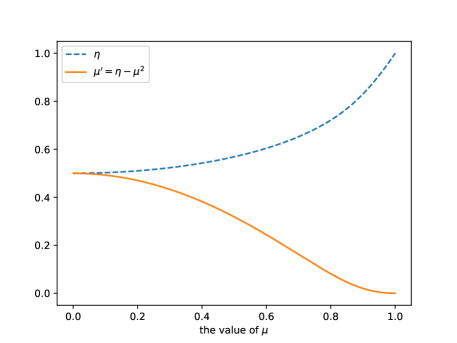
Figure 1: The graphs of $\eta$ and $\eta-\mu^{2}$ as functions of $\mu$

In our numerical experiments the Newton iteration usually terminate in 3 or 4 steps. In Figure 2, we show the amplitudes of Legendre coefficients calculated using above procedure where we take $n_{l}=150$ and $N=200$ in (3.39) and (3.40). From this figure, we see that the Legendre expansion has spectral accuracy and the error is about $10^{-18}$ when 125 expansion terms are used.

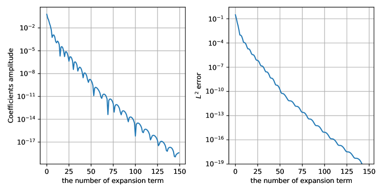
Figure 2: The coefficients amplitude(left) and the estimated $L^{2}$ error (right) of Legendre expansion of $\eta(\mu)$

After the coefficients of the Legendre expansion of $\eta(\mu)$ are pre-calculated, we can easily obtain the elements in the transformed fourth order moment by Eq. (3.30). Then, as the last step of moment closure approximation, the components of the forth order moments in original coordinates can be calculated by:

$$\hat{q}_{ijkl}=\sum_{i^{\prime},j^{\prime},k^{\prime},l^{\prime}}U_{ii^{\prime}}U_{jj^{\prime}}U_{kk^{\prime}}U_{ll^{\prime}}{q}_{i^{\prime}j^{\prime}k^{\prime}l^{\prime}},$$ (3.43)

where $U_{ij}$ are the components of the transform matrix $U$ defined in Eq. (3.37).

The overall moment closure procedure for symmetric QEA on unit circle is summarized in Algorithm 1.

Algorithm 1 Calculate the fourth order moments for symmetric QEA on unit circle

Input: The values of the elements in second order moment $\hat{M}$.
Output: The values of the elements in fourth order moment $\hat{Q}$.

0:  Pre-calculated coefficients $\{b_{k},k=0,\ldots,n_{l}\}$ of the Legendre expansion of $\eta(\mu)$.

1:  Transform $\hat{M}$ into a diagonalized matrix $M=U^{T}\hat{M}U$, where $U$ is given by (3.37).

2:  Calculate $\mu=m_{11}-m_{22}$ where $m_{11}$ and $m_{22}$ are the diagonal elements in $M$.

3:  Map the value of $\mu$ to $x\in[-1,1]$ with $x=2\mu-1$.

4:  Use the Legendre expansion given in Eq.(3.39) to calculate the value of $\eta$.

5:  Evaluate the values of $q_{0}$, $q_{2}$ and $q_{4}$ by Eq.(3.30), then use the definition (3.26) and (3.25) to calculate $q_{ijkl}$ and use (3.43) to calculate $\hat{Q}=(\hat{q}_{ijkl})$.

Remark 3

The overall storage cost in Algorithm 1 is $O(n_{l}+m)$, and the computational time cost is $O(mn_{l})$, where $n_{l}$ is the number of Legendre coefficients and $m$ is the number of fourth-order moment tensors to be evaluated. For $n_{l}\leq 125$, the evaluation of (3.39) can be done by fast matrix-vector product on modern computers.

Note that it is possible to further reduce the computational time cost by using a piecewise polynomial approximation. For example, if we divide the range of $\mu\in$ [0,1] into 6 intervals: $[0,0.5],[0.5,0.73],[0.73,0.84],[0.84,0.91],[0.91,0.96],[0.96,1]$. Then the numbers of Legendre expansion terms $n_{l}$ can be significantly reduced for maintaining similar $L^{2}$ error of approximating $\eta(\mu)$ in each interval. The result is shown in Table 1. We see double precision is achieved on all six intervals with less than 20 Legendre coefficients, which leads to an overall computational time cost reduction by a factor of 5. One can divide the interval into more pieces to further reduce the computational cost. For simplicity, we will not present more results here.

Table 1: Piecewise Legendre approximation of $\eta(\mu)$.

Interval	$n_{l}$	$L^{2}$ error
$[0,0.5]$	19	7.34E-18
$[0.5,0.73]$	19	2.30E-18
$[0.73,0.84]$	18	5.45E-18
$[0.84,0.91]$	18	7.64E-18
$[0.91,0.96]$	18	8.97E-18
$[0.96,1]$	18	5.41E-18

4 Symmetric QEA on unit sphere

The overall moment closure procedure based on symmetric QEA on unit sphere is similar to that on unit circle. For simplicity we first consider the diagonalized case.

We consider the diagonalized 3-dimensional problem on unit sphere $\Omega=\{\,{\bf m}\in\mathbb{R}^{3},\,|{\bf m}|=1\,\}$. We consider two different cases: the uniaxial case, where two of the three eigenvalues of $B$ tensor are equal, and the biaxial case where three eigenvalues of $B$ tensor are all different. Since $f_{B+cI}$ is identical to $f_{B}$, we can use a particular shift $cI$ to make the $B$ in uniaxial case be $\operatorname*{diag}(0,0,-2\lambda)$, make the $B$ in biaxial case $\operatorname*{diag}(-\lambda_{1}-\lambda_{2},-\lambda_{1}+\lambda_{2},0)$. Here $\lambda_{1}\geq\lambda_{2}\geq 0$. We first consider the uniaxial case, which is easier to implement.

4.1 The uniaxial case

For the uniaxial case, we set $B=\mathrm{diag}(0,0,-2\lambda)$, $\lambda\in\mathbb{R}$. For $\lambda>0$, $f_{B}({\bf m})$ is an oblate distribution, while $\lambda<0$, it is prolate. By using spherical coordinates ${\bf m}=(\sin\theta\cos\varphi,\sin\theta\sin\varphi,\cos\theta)$ with $0\leq\theta\leq\pi$, $0\leq\varphi\leq 2\pi$, we have

$$m_{ij}=\int_{0}^{\pi}\int_{0}^{2\pi}\frac{1}{z}\exp[-2\lambda\cos^{2}\theta]{\bf m}_{i}{\bf m}_{j}\sin\theta\mathrm{d}\theta\mathrm{d}\varphi,\quad i,j=1,2,$$

where

$$z(\lambda)=\int_{0}^{\pi}\int_{0}^{2\pi}\exp[-2\lambda\cos^{2}\theta]\sin\theta{\rm{d}}\theta{\rm{d}}\varphi.$$ (4.44)

It is easy to check that $m_{ij}=0$ if $i\neq j$. The nonzero terms left are $m_{11}$, $m_{22}$ and $m_{33}$. We define

$$\mu(\lambda):=-\frac{z^{\prime}(\lambda)}{z(\lambda)}=\frac{1}{z(\lambda)}\int_{0}^{\pi}\int_{0}^{2\pi}\exp[-2\lambda\cos^{2}\theta]2\cos^{2}\theta\sin\theta{\rm{d}}\theta{\rm{d}}\varphi.$$ (4.45)

Then

$$\mu^{\prime}(\lambda)=-\frac{z^{\prime\prime}(\lambda)}{z(\lambda)}+\big{(}\frac{z^{\prime}(\lambda)}{z(\lambda)}\big{)}^{2}=\mu^{2}(\lambda)-\frac{z^{\prime\prime}(\lambda)}{z(\lambda)}.$$ (4.46)

And the second order moments are related to $\mu$ by

$$m_{33}=\frac{\mu}{2},\quad m_{11}=m_{22}=\frac{2-\mu}{4}.$$ (4.47)

The fourth order moments are defined as

$$q_{ijkl}=\int_{0}^{\pi}\int_{0}^{2\pi}\frac{1}{z(\lambda)}\exp[-2\lambda\cos^{2}\theta]{\bf m}_{i}{\bf m}_{j}{\bf m}_{k}{\bf m}_{l}\sin\theta{\rm{d}}\theta{\rm{d}}\varphi,\quad i,j,k,l=1,2,3.$$

One may check that only the following several terms: $q_{1111}$, $q_{2222}$, $q_{3333}$, $q_{1122}$, $q_{1133}$, $q_{2233}$ are nonzero, and they satisfy following constraints

$$\left(\begin{array}[]{ccc}1&1&0\\ 1&0&1\\ 0&1&1\end{array}\right)\left(\begin{array}[]{c}q_{1122}\\ q_{1133}\\ q_{2233}\end{array}\right)=\left(\begin{array}[]{c}m_{11}-q_{1111}\\ m_{22}-q_{2222}\\ m_{33}-q_{3333}\end{array}\right).$$ (4.57)

Actually, there is only one independent variable in forth order moments. Let’s define it as

$$\eta(\lambda)=\frac{z^{\prime\prime}(\lambda)}{z(\lambda)}=\frac{1}{z(\lambda)}\int_{0}^{\pi}\int_{0}^{2\pi}\exp[-2\lambda\cos^{2}\theta]4\cos^{4}\theta\sin\theta{\rm{d}}\theta{\rm{d}}\varphi.$$ (4.58)

It follows from (4.46) that

$$\mu^{\prime}(\lambda)=\mu^{2}(\lambda)-\eta(\lambda).$$ (4.59)

Similar to Theorem 3.1, one can prove that $\mu^{\prime}(\lambda)$ is positive by using the Cauchy-Schwarz inequality. By using the definitions, the symmetry between $m_{1}$ and $m_{2}$, the relation (4.57), we find that fourth order moments are related to $\eta$ and $\mu$ by:

$$q_{3333}=\frac{\eta}{4},\quad q_{1133}=q_{2233}=\frac{\mu}{4}-\frac{\eta}{8},\quad q_{1111}=q_{2222}=3q_{1122}=\frac{3}{8}(1-\mu)+\frac{3}{32}\eta.$$ (4.60)

To efficiently evaluate $z(\lambda)$, we rewrite it by using Eq. (4.44) as

$$z(\lambda) =4\pi\int_{0}^{\frac{\pi}{2}}\exp[-2\lambda\cos^{2}\theta]\sin\theta{\rm{d}}\theta$$

$$=4\pi\int_{0}^{1}\exp[-2\lambda t^{2}]{\rm{d}}t$$

$$=2\pi\int_{0}^{1}\exp[-2\lambda x]x^{-\frac{1}{2}}{\rm{d}}x$$

$$=2\pi\frac{\Gamma(1)\Gamma(\frac{1}{2})}{\Gamma(\frac{3}{2})}\ _{1}F_{1}(\frac{1}{2};\frac{3}{2};-2\lambda)$$

$$=4\pi\ _{1}F_{1}(\frac{1}{2};\frac{3}{2};-2\lambda),$$ (4.61)

where

$$_{1}F_{1}(a;b;\lambda)=\frac{\Gamma(b)}{\Gamma(a)\Gamma(b-a)}\int_{0}^{1}\exp(\lambda x)x^{a-1}(1-x)^{b-a-1}{\rm{d}}x$$ (4.62)

is the confluent hypergeometric function (olver_nist_2010, , Chapter 13). Similarly, we have

$$\mu(\lambda)=\frac{8\pi}{3z}\ _{1}F_{1}(\frac{3}{2};\frac{5}{2};-2\lambda),$$ (4.63)

$$\eta(\lambda)=\frac{16\pi}{5z}\ _{1}F_{1}(\frac{5}{2};\frac{7}{2};-2\lambda).$$ (4.64)

We use the function hyp1f1(a,b,z) in MPmath johansson_mpmath_2020 to calculate the confluent hypergeometric function ${}_{1}F_{1}$ with high accuracy.

Then, as done in the 2-dimensional case, we consider an Legendre polynomial approximation of $\eta(\mu)$ as a function of $\mu$, which is similar to Eq.(3.39), but here $x=\mu-1$ since $\mu\in[0,{2}]$. We use again Newton’s method to find the $\lambda$ values that produce $\mu(\lambda)$ on mapped Legendre-Gauss points, then use these $\lambda$ values to calculate corresponding $\mu$ and $\eta$ values, and use them to obtain Legendre coefficients. We take $n_{l}=160$ and use $N=200$ Legendre-Gauss points to compute the coefficients of the Legendre polynomial approximation. The result is given in Figure 3, from which we see that the Legendre expansion has spectral accuracy and the $L^{2}$ error is reduced to about $10^{-16}$ (smaller than double precision $2.2\times 10^{-16}$) with less than 150 expansion terms are used.

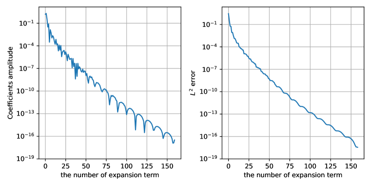
Figure 3: The coefficients (left) and the $L^{2}$ error (right) of Legendre expansion of $\eta$

After the coefficients of the Legendre approximation of $\eta(\mu)$ is obtained, we can efficiently calculate $\eta$ for given $\mu$, and then obtain the elements in fourth order moment by (4.60). The overall procedure is very similar to Algorithm 1 for the two dimensional case.

About 150 global Legendre terms are needed to obtain double precision, which means the computational cost for evaluating $m$ fourth order moments is about $O(n_{l}m)$, where $n_{l}\approx 150$. We can further reduce the computational cost by using piecewise polynomial approximations. For example, we can divide the range of $\mu\in$ $[0,{2}]$ into multiple intervals, then use Legendre expansions to approximate $\eta(\mu)$ on each interval. The number of expansion terms $n$ and the $L^{2}$ approximation errors on each interval are showed in Table 2. We see that with only 18 expansion terms, the $L^{2}$ approximation error can be reduced to less than $4\times 10^{-17}$ on all intervals. Note that $\mu=2/3$ corresponds to the special case where $m_{11}=m_{22}=m_{33}$. So the first 5 intervals in Table 2 are oblate cases, while the last 6 intervals are prolate cases.

Table 2: Piecewise Legendre approximation for the uniaxial Bingham closure on sphere.

Interval	$n_{l}$	$L^{2}$ error
$[0,0.045]$	18	1.41E-17
$[0.045,0.103]$	18	2.34E-17
$[0.103,0.2]$	18	2.88E-17
$[0.2,0.36]$	18	1.69E-17
$[0.36,\frac{2}{3}]$	18	3.42E-17
$[\frac{2}{3},1.26]$	18	1.28E-17
$[1.26,1.56]$	18	1.13E-17
$[1.56,1.73]$	18	1.26E-17
$[1.73,1.84]$	18	1.38E-17
$[1.84,1.925]$	18	1.80E-17
$[1.925,2]$	18	1.89E-17

4.2 The biaxial case

In biaxial case, we take $B=\operatorname*{diag}(-\lambda_{1}-\lambda_{2},-\lambda_{1}+\lambda_{2},0)$, where $\lambda_{1}>\lambda_{2}>0$. Note that the limit cases $\lambda_{2}=0$ and $\lambda_{2}\rightarrow\infty$ are reduced to uniaxial distribution. By using spherical coordinates ${\bf m}=(\sin\theta\cos\varphi,\sin\theta\sin\varphi,\cos\theta)$ with $0\leq\theta\leq\pi$, $0\leq\varphi\leq 2\pi$, we have

$$m_{ij}=\int_{0}^{\pi}\int_{0}^{2\pi}\frac{1}{z}\exp[-(\lambda_{1}+\lambda_{2}\cos(2\varphi))\sin^{2}\theta]{\bf m}_{i}{\bf m}_{j}\sin\theta\mathrm{d}\theta\mathrm{d}\varphi,\quad i,j=1,2,$$

where

$$z(\lambda_{1},\lambda_{2})=\int_{0}^{\pi}\int_{0}^{2\pi}\exp[-(\lambda_{1}+\lambda_{2}\cos(2\varphi))\sin^{2}\theta]\sin\theta\mathrm{d}\theta\mathrm{d}\varphi.$$ (4.65)

By the definition of $B$, we have $m_{11}\leq m_{22}\leq m_{33}$. It is easy to check that $m_{ij}=0$ if $i\neq j$ by symmetry or direct integration. The nonzero second order moments are $m_{11}$, $m_{22}$ and $m_{33}$, with constraint $m_{11}+m_{22}+m_{33}=1$, so we have two independent variables. We take them as

$$\mu_{1}(\lambda_{1},\lambda_{2}) =-\frac{\partial z}{\partial\lambda_{1}}\frac{1}{z}=\frac{1}{z}\int_{0}^{\pi}\int_{0}^{2\pi}\exp[-(\lambda_{1}+\lambda_{2}\cos(2\varphi))\sin^{2}\theta]\sin^{3}\theta{\rm{d}}\theta{\rm{d}}\varphi,$$ (4.66)

$$\mu_{2}(\lambda_{1},\lambda_{2}) =-\frac{\partial z}{\partial\lambda_{2}}\frac{1}{z}=\frac{1}{z}\int_{0}^{\pi}\int_{0}^{2\pi}\exp[-(\lambda_{1}+\lambda_{2}\cos(2\varphi))\sin^{2}\theta]\cos(2\varphi)\sin^{3}\theta{\rm{d}}\theta{\rm{d}}\varphi.$$ (4.67)

Variables $\mu_{1},\mu_{2}$ are related to second order moments $m_{11},m_{22}$ by

$$\mu_{1}=m_{11}+m_{22},\quad\mu_{2}=m_{11}-m_{22}.$$ (4.68)

The fourth order moments are defined as

$$q_{ijkl}=\int_{0}^{\pi}\int_{0}^{2\pi}\frac{1}{z(\lambda)}\exp[-(\lambda_{1}+\lambda_{2}\cos(2\varphi))\sin^{2}\theta]{\bf m}_{i}{\bf m}_{j}{\bf m}_{k}{\bf m}_{l}\sin\theta\text{d}\theta\text{d}\varphi,\quad i,j,k,l=1,2,3.$$

It is easy to check that the nonzero terms are: $q_{1111}$, $q_{2222}$, $q_{3333}$, $q_{1122}$, $q_{1133}$, $q_{2233}$. They satisfy the relation

$$\left(\begin{array}[]{ccc}1&1&0\\ 1&0&1\\ 0&1&1\end{array}\right)\left(\begin{array}[]{c}q_{1122}\\ q_{1133}\\ q_{2233}\end{array}\right)=\left(\begin{array}[]{c}m_{11}-q_{1111}\\ m_{22}-q_{2222}\\ m_{33}-q_{3333}\end{array}\right).$$ (4.78)

So there are three independent variables. We define them as

$$\eta_{1}(\lambda_{1},\lambda_{2}) =\frac{1}{z}\frac{\partial^{2}z}{\partial\lambda_{1}^{2}}=\frac{1}{z}\int_{0}^{\pi}\int_{0}^{2\pi}\exp[-(\lambda_{1}+\lambda_{2}\cos 2\varphi)\sin^{2}\theta]\sin^{5}\theta{\rm{d}}\theta{\rm{d}}\varphi$$ (4.79)

$$\eta_{2}(\lambda_{1},\lambda_{2}) =\frac{1}{z}\frac{\partial^{2}z}{\partial\lambda_{1}\partial\lambda_{2}}=\frac{1}{z}\int_{0}^{\pi}\int_{0}^{2\pi}\exp[-(\lambda_{1}+\lambda_{2}\cos 2\varphi)\sin^{2}\theta]\cos(2\varphi)\sin^{5}\theta{\rm{d}}\theta{\rm{d}}\varphi$$ (4.80)

$$\eta_{3}(\lambda_{1},\lambda_{2}) =\frac{1}{z}\frac{\partial^{2}z}{\partial\lambda_{2}^{2}}=\frac{1}{z}\int_{0}^{\pi}\int_{0}^{2\pi}\exp[-(\lambda_{1}+\lambda_{2}\cos 2\varphi)\sin^{2}\theta]\cos^{2}(2\varphi)\sin^{5}\theta{\rm{d}}\theta{\rm{d}}\varphi$$ (4.81)

From the relation between $\mu(\lambda)$ and $\eta(\lambda)$, we derive that

$$\begin{split}\left\{\begin{array}[]{cll}\eta_{1}=&\mu_{1}^{2}-\frac{\partial\mu_{1}}{\partial\lambda_{1}},&\\ \eta_{2}=&\mu_{1}\mu_{2}-\frac{\partial\mu_{1}}{\partial\lambda_{2}}=&\mu_{1}\mu_{2}-\frac{\partial\mu_{2}}{\partial\lambda_{1}},\\ \eta_{3}=&\mu_{2}^{2}-\frac{\partial\mu_{2}}{\partial\lambda_{2}},&\end{array}\right.\end{split}$$ (4.82)

which will be used to compute the Jacobi matrix in the Newton’s method.

Theorem 4.1

The Jacobi matrix of $\frac{\partial(\mu_{1},\mu_{2})}{\partial(\lambda_{1},\lambda_{2})}$ is negative semi-definite.

Proof

To show the Jacobi matrix $\frac{\partial(\mu_{1},\mu_{2})}{\partial(\lambda_{1},\lambda_{2})}$ is negative semi-definite, we first define function $f(\lambda_{1},\lambda_{2})=\log(z(\lambda_{1},\lambda_{2}))$. Since

$$\left(\begin{array}[]{cc}\frac{\partial^{2}f(\lambda_{1},\lambda_{2})}{\partial\lambda_{1}^{2}}&\frac{\partial^{2}f(\lambda_{1},\lambda_{2})}{\partial\lambda_{1}\partial\lambda_{2}}\\ \frac{\partial^{2}f(\lambda_{1},\lambda_{2})}{\partial\lambda_{1}\partial\lambda_{2}}&\frac{\partial^{2}f(\lambda_{1},\lambda_{2})}{\partial\lambda_{2}^{2}}\end{array}\right)=-\left(\begin{array}[]{cc}\frac{\partial\mu_{1}}{\partial\lambda_{1}}&\frac{\partial\mu_{1}}{\partial\lambda_{2}}\\ \frac{\partial\mu_{2}}{\partial\lambda_{1}}&\frac{\partial\mu_{2}}{\partial\lambda_{2}}\end{array}\right),$$

we only need to show that $f(\lambda_{1},\lambda_{2})$ is a convex function, or to show that for any given $\lambda_{1}\geq\lambda_{2}\geq 0$, $a^{2}+b^{2}=1$, $f(\lambda_{1}+\gamma a,\lambda_{2}+\gamma b)$ as a function of $\gamma$ is convex. By direct calculation, we have

$$\frac{{\rm{d}}^{2}f}{{\rm{d}}\gamma^{2}}=\frac{1}{z^{2}}\Big{[}z\frac{{\rm{d}}^{2}z}{{\rm{d}}\gamma^{2}}-(\frac{{\rm{d}}z}{{\rm{d}}\gamma})^{2}\Big{]},$$

where

$$z(\gamma)=\int_{0}^{\pi}\int_{0}^{2\pi}\exp[-(\lambda_{1}+\lambda_{2}\cos(2\varphi)+\gamma(a+b\cos 2\varphi))\sin^{2}\theta]\sin\theta\mathrm{d}\theta\mathrm{d}\varphi.$$ (4.83)

Similar to Theorem 3.1, by using Cauchy-Schwartz inequality, we have $({\rm{d}}z/{\rm{d}}\gamma)^{2}\leq z({\rm{d}}^{2}z/{\rm{d}}\gamma^{2})$, which means $f$ as a function of $\gamma$ is convex. The theorem is proved. ∎

Given the values of $\mu_{1}$, $\mu_{2}$ and $\eta_{1}$, $\eta_{2}$, $\eta_{3}$, the second order and forth order moments of the biaxial Bingham distribution can be obtained by

$$m_{11}=\frac{\mu_{1}+\mu_{2}}{2},\quad m_{22}=\frac{\mu_{1}-\mu_{2}}{2},\quad m_{33}=1-\mu_{1},$$ (4.84)

$$\begin{split}&q_{1111}=\frac{\eta_{1}+2\eta_{2}+\eta_{3}}{4},\quad q_{1122}=\frac{\eta_{1}-\eta_{3}}{4},\quad q_{2222}=\frac{\eta_{1}-2\eta_{2}+\eta_{3}}{4},\\ &q_{1133}=\frac{(\mu_{1}+\mu_{2})-(\eta_{1}+\eta_{2})}{2},\quad q_{2233}=\frac{(\mu_{1}-\mu_{2})-(\eta_{1}-\eta_{2})}{2},\\ &q_{3333}=1-2\mu_{1}+\eta_{1}.\end{split}$$ (4.85)

Now we describe how to efficiently calculate $z,\mu_{1},\mu_{2},\eta_{1},\eta_{2},\eta_{3}$ and do the moment closure approximation.

Similar to the uniaxial case, the partition function and moments can be written as integrations of confluent hypergeometric functions. Since for large and close $\lambda_{1},\lambda_{2}$ values, the integrands ${}_{1}F_{1}(a;b;-(\lambda_{1}+\lambda_{2}\cos(2\varphi)))$ are localized at $\cos(2\varphi)\approx-1$, we use Legendre-Gauss quadrature to do numerical integration in $\varphi$ variable to put more grid points near $\cos(2\varphi)\approx-1$. To this end, we write those quantities as:

$$z(\lambda_{1},\lambda_{2})=2\int_{0}^{2\pi}\!{}_{1}F_{1}(1;\frac{3}{2};-(\lambda_{1}+\lambda_{2}\cos 2\varphi)){\rm{d}}\varphi=2\pi\int^{1}_{-1}\!{}_{1}F_{1}(1;\frac{3}{2};-(\lambda_{1}+\lambda_{2}\cos\pi t)){\rm{d}}t$$ (4.86)

$$\mu_{1}(\lambda_{1},\lambda_{2})=\frac{4\pi}{3z}\int_{-1}^{1}\ {}_{1}F_{1}(2;\frac{5}{2};-(\lambda_{1}+\lambda_{2}\cos\pi t)){\rm{d}}t,$$ (4.87)

$$\mu_{2}(\lambda_{1},\lambda_{2})=\frac{4\pi}{3z}\int_{-1}^{1}\ {}_{1}F_{1}(2;\frac{5}{2};-(\lambda_{1}+\lambda_{2}\cos\pi t))\cos({\pi}t){\rm{d}}t,$$ (4.88)

$$\eta_{1}(\lambda_{1},\lambda_{2})=\frac{16\pi}{15z}\int_{-1}^{1}\ {}_{1}F_{1}(3;\frac{7}{2};-(\lambda_{1}+\lambda_{2}\cos\pi t)){\rm{d}}t,$$ (4.89)

$$\eta_{2}(\lambda_{1},\lambda_{2})=\frac{16\pi}{15z}\int_{-1}^{1}\ {}_{1}F_{1}(3;\frac{7}{2};-(\lambda_{1}+\lambda_{2}\cos\pi t))\cos({\pi}t){\rm{d}}t,$$ (4.90)

$$\eta_{3}(\lambda_{1},\lambda_{2})=\frac{16\pi}{15z}\int_{-1}^{1}\ {}_{1}F_{1}(3;\frac{7}{2};-(\lambda_{1}+\lambda_{2}\cos\pi t)){\cos^{2}(\pi t)}{\rm{d}}t,$$ (4.91)

where ${}_{1}F_{1}$ is defined in (4.62), they are evaluated using the function hyp1f1(a,b,z) in MPmath to get high accuracy. Since the integrands are all even functions, we can use half the Gauss points to save computational time.

(a) The region of $\mu_{1}$ and $\mu_{2}$

(b) The region of $x$ and $y$

Figure 4: The transformation between the triangular and rectangular domains

We have shown how to calculate $\mu_{1},\mu_{2}$, $\eta_{1},\eta_{2}$ and $\eta_{3}$ for given $\lambda$. Next, we show how to efficiently calculate $\eta_{1},\eta_{2}$ and $\eta_{3}$ for given $\mu_{1},\mu_{2}$. Similar to the 2-dimensional case, we use Legendre method to approximate functions $\tilde{\eta}_{i}(\mu_{1},\mu_{2}),i=1,2,3$. Since the domain of $(\mu_{1},\mu_{2})$, shown in Figure 4(a), is not of tensor product form, we first transform it into standard domain $[-1,1]^{2}$ by using following mapping

$$\left\{\begin{array}[]{ccc}\mu_{1}&=&\frac{(1+x)(1-y)}{8}+\frac{y}{3}+\frac{1}{3},\\ \mu_{2}&=&-\frac{(1+x)(1-y)}{8}.\end{array}\right.$$ (4.94)

The corresponding inverse mapping is

$$\left\{\begin{array}[]{ccc}x&=&\frac{8\mu_{2}}{3\mu_{1}+3\mu_{2}-2}-1,\\ y&=&3\mu_{1}+3\mu_{2}-1.\end{array}\right.$$ (4.97)

where $x\in[-1,1]$, $y\in[-1,1]$. Then we use Legendre-Gauss points in the transformed domain to calculate the Legendre approximation coefficients. Denote the Legendre approximation of $\tilde{\eta}_{i}(\mu_{1},\mu_{2})$ as

$$\eta_{i}(\lambda_{1},\lambda_{2})=\tilde{\eta}_{i}(\mu_{1},\mu_{2})=\hat{\eta}(x,y)\approx\sum_{s=0}^{n_{1}}\sum_{t=0}^{n_{2}}b^{i}_{st}L_{s}(x)L_{t}(y),\quad i=1,2,3,$$ (4.98)

where

$$\begin{split}b^{i}_{st}&=\frac{1}{\gamma_{s}\gamma_{t}}\sum_{i=0}^{N_{1}}\sum_{j=0}^{N_{2}}\hat{\eta}(x_{i},y_{j})L_{s}(x_{i})L_{t}(y_{j})\omega_{i}\omega_{j},\end{split}$$ (4.99)

with $\gamma_{s}=\frac{2}{2s+1}$, $\gamma_{t}=\frac{2}{2t+1}$, $\{x_{i},\omega_{i}\}_{i=0}^{N_{1}}$ and $\{y_{j},\omega_{j}\}_{j=0}^{N_{2}}$ are the Legendre-Gauss quadrature points and weights.

Again, we use Newton’s method to obtain the values of $\lambda_{1},\lambda_{2}$ that produce Legendre-Gauss points in $x,y$ domain:

$$\lambda^{k+1}=\lambda^{k}-J_{F}(\lambda^{k})^{-1}F(\lambda^{k})$$ (4.100)

where $\lambda^{k}=(\lambda_{1}^{k},\lambda_{2}^{k})$, $F(\lambda^{k})=\mu^{*}-\mu(\lambda^{k})$, $\mu^{*}$ is the image of Legendre-Gauss point $(x_{i},y_{j})$ under mapping (4.94). $J_{F}(\lambda^{k})$ is the Jacobi matrix:

$$J_{F}(\lambda^{k})=-J_{\mu}(\lambda^{k})=-\left.\left(\begin{array}[]{cc}\frac{\partial\mu_{1}}{\partial\lambda_{1}}&\frac{\partial\mu_{1}}{\partial\lambda_{2}}\\ \frac{\partial\mu_{2}}{\partial\lambda_{1}}&\frac{\partial\mu_{2}}{\partial\lambda_{2}}\end{array}\right)\right|_{(\lambda_{1},\lambda_{2})=(\lambda_{1}^{k},\lambda_{2}^{2})}.$$

Then equation (4.100) can be rewritten as

$$\lambda^{k+1}=\lambda^{k}+J_{\mu}(\lambda^{k})^{-1}(\mu^{*}-\mu(\lambda^{k})).$$

The derivatives in Jacobi matrix $J_{\mu}(\lambda)$ can be removed by using (4.82). Similar to the 2-dimensional case, we use a table to find closed $\lambda$ points to initialize Newton’s method and the iteration is terminated if the $L^{2}$ distance of the objective functions between two adjacent iterations is smaller than a given tolerance. The tolerance we used here is $10^{-15}$. According to Theorem 4.1, the Newton iteration is well-defined, the system corresponds to a convex optimization problem. We expect a global convergence as in the 2-dimensional case. Our numerical results show that the iterations usually terminate in less than 20 steps.

In Figure 5, we show the coefficients and $L^{2}$ error of the Legendre approximations of $\eta_{1}$, $\eta_{2}$ and $\eta_{3}$, where we take $n_{1}=100$, $n_{2}=100$ and $N_{1}=N_{2}=100$ in (4.98) and (4.99). The results suggest that the Legendre expansion has spectral accuracy and the error is about $10^{-15}$ when $n_{1}=90$, $n_{2}=75$.

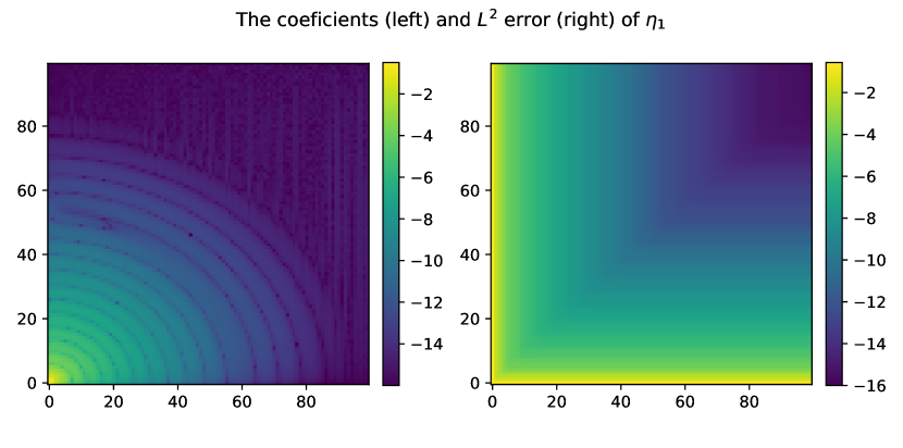
Figure 5: The coefficients (left) and the $L^{2}$ error of the Legendre approximation of $\eta_{1}$, $\eta_{2}$, $\eta_{3}$

After the coefficients $b_{st}^{i}$ of the Legendre approximation are pre-calculated, we can efficiently calculate $\eta_{i},i=1,2,3$ by matrix-matrix multiplication for given values of $\mu_{1},\mu_{2}$. The other elements in forth order moment tensor under diagonalized coordinates can be obtained by (LABEL:eq:re_qandeta). All the fourth order moments under original coordinates can be obtained by a coordinate transform. The overall moment closure procedure is summarized in Algorithm 2.

Algorithm 2 Calculate forth order moments for symmetric QEA on unit sphere

Input: The values of the elements in second order moment $\hat{M}$
Output: The values of the elements in fourth order moment $\hat{Q}$

0:  Pre-calculated coefficients $\{\,b_{st}^{i},s=0,\ldots,n_{1},t=0,\ldots,n_{2},i=1,2,3\,\}$

1:  Use a linear algebra subroutine to calculate an orthogonal matrix $U$ which is formed by eigenvectors of $\hat{M}$ and make $M=U^{T}\hat{M}U$ into a diagonal matrix with $m_{11}\leq m_{22}\leq m_{33}$.

2:  Calculate the value of $\mu_{1},\mu_{2}$ from $m_{11},m_{22}$ by using (4.68).

3:  Mapping the values of $\mu_{1}$ and $\mu_{2}$ to $x\times y\in[-1,1]\times[-1,1]$ with the transformation in Eq.(4.97)

4:  Calculate the values of $\eta_{1}$, $\eta_{2}$ and $\eta_{3}$ by Eq.(4.98)

5:  Calculate the nonzero elements in forth order moment under diagonalized coordinates by Eq.(LABEL:eq:re_qandeta).

6:  Use (3.43) to calculate the elements in $\hat{Q}=(\hat{q}_{ijkl})$.

The overall computational time cost for evaluating $m$ moments in Algorithm 2 is $O(n_{1}n_{2}m)$. Here, $n_{1},n_{2}$ is about $70\sim 90$ to reach double precision. The storage cost is $O(n_{1}n_{2}+(n_{1}+n_{2})m)$. To reduce the computational time cost, we may use piecewise Legendre approximation. To show this, we divide the region of $(x,y)\in[-1,1]^{2}$ into 6 blocks. These 6 blocks in $(x,y)$ are showed in Figure 6(b) marked by 6 different colors, and the corresponding blocks in $(\mu_{1},\mu_{2})$ are shown in Figure 6(a). The coordinates of corner points in $(\mu_{1},\mu_{2})$ blocks are given below:

$$A_{1}(0,0),\quad A_{2}(\frac{1}{2},-\frac{1}{2}),\quad A_{3}(\frac{2}{3},0),\quad B_{1}(\frac{1}{3},0),\quad B_{2}(\frac{5}{12},-\frac{1}{12}),\quad B_{3}(\frac{7}{12},-\frac{1}{4}),$$

$$C_{1}(\frac{1}{9},0),\quad C_{2}(\frac{11}{72},-\frac{1}{24}),\quad C_{3}(\frac{1}{4},-\frac{6}{35}),\quad C_{4}(\frac{19}{36},-\frac{5}{12}),\quad D_{1}(\frac{1}{20},-\frac{1}{20}),\quad D_{2}(\frac{1}{6},-\frac{1}{6}).$$

(a) The partition formed by $\mu_{1}$ and $\mu_{2}$

(b) The partition formed by $x$ and $y$

Figure 6: Partitions of parameter regions for piecewise Legendre approximations

We apply the Legendre approximation for each blocks in such a partition. The number of expansion terms $n_{1}$, $n_{2}$ and the corresponding $L^{2}$ error for $\eta_{1}$, $\eta_{2}$ and $\eta_{3}$ in each block are shown in Table 3. We see that $n_{1}$ and $n_{2}$ are both no more than 26 with the $L^{2}$ error gets below $10^{-14}$ in these blocks. Comparing to the global Legendre expansion in the whole region, the piecewise Legendre expansions greatly reduce the time cost of calculation.

Table 3: The number of expansion terms $n_{1}$, $n_{2}$ and the $L^{2}$ error for $\eta_{1}$, $\eta_{2}$ and $\eta_{3}$ in each block with piecewise Legendre approximation.

Block	$\eta_{1}$			$\eta_{2}$			$\eta_{3}$
	$n_{1}$	$n_{2}$	$L^{2}$ error	$n_{1}$	$n_{2}$	$L^{2}$ error	$n_{1}$	$n_{2}$	$L^{2}$ error
	17	15	7.26E-15	17	15	9.27E-15	17	16	9.07E-15
	22	22	4.88E-15	22	21	6.48E-15	23	21	9.78E-15
	16	20	6.11E-15	16	20	3.99E-15	16	21	8.18E-15
	24	26	9.77E-15	23	26	8.63E-15	23	26	7.68E-15
	23	24	9.71E-15	23	25	9.46E-15	22	26	8.04E-15
	20	24	9.72E-15	21	24	6.23E-15	22	25	9.69E-15

5 Summary

We have shown some basic properties of quasi-equilibrium closure approximation for antipodally symmetric problems and designed efficient high order numerical implementations for such closure approximations on unit circle and unit sphere by using global Legendre approximation and piecewise Legendre approximation. The proposed implementation can reach to double accuracy with mush smaller memory cost. The time efficiency is improved by using piecewise polynomial approximations. The proposed approach can be directly extended to handle other QEA closure approximations, such as the Fisher-Bingham kent_fisherbingham_1982 and von Mises-Fisher distributionssra_short_2012 for non-symmetric problems.

Note that the tensor-product polynomial approximations are limited to low-dimensional problems. For high-dimensional problems, spectral sparse grid methods (see e.g. shen_efficient_2010 shen_efficient_2012 ) and deep neural networks li_better_2020 yu_onsagernet_2020 are vital approximation tools. Implementation of high-dimensional QEA using these techniques will be the topic of our future study.

Code and data availability All data and code generated or used during the study are available from the corresponding author by request.

References

- [1] Milton Abramowitz and Irene A. Stegun. Handbook of Mathematical Functions with Formulas, Graphs, and Mathematical Tables. U.S. Department of Commerce, 1972.
- [2] Christopher Bingham. An antipodally symmetric distribution on the sphere. Ann. Stat., 2(6):1201–1225, 1974.
- [3] Charu V. Chaubal and L. Gary Leal. A closure approximation for liquid-crystalline polymer models based on parametric density estimation. J. Rheol., 42(1):177, 1998.
- [4] J. S. Cintra Jr and C. L. Tucker III. Orthotropic closure approximations for flow-induced fiber orientation. J. Rheol., 39:1095, 1995.
- [5] M. Doi and S. F. Edwards. The Theory of Polymer Dynamics. Oxford University Press, USA, 1986.
- [6] J. Feng, C. V. Chaubal, and L. G. Leal. Closure approximations for the Doi theory: Which to use in simulating complex flows of liquid-crystalline polymers? J. Rheol., 42:1095, 1998.
- [7] J. Willard Gibbs. Elementary Principles in Statistical Mechanics. Charles Scribner’s Sons, 1902.
- [8] Alexander Gorban and Ilya V. Karlin. Invariant Manifolds for Physical and Chemical Kinetics, volume 660 of Lecture Notes in Physics. Springer Berlin Heidelberg, Berlin, Heidelberg, 2005.
- [9] Alexander N. Gorban, Iliya V. Karlin, Patrick Ilg, and Hans Christian Öttinger. Corrections and enhancements of quasi-equilibrium states. Journal of Non-Newtonian Fluid Mechanics, 96(1):203–219, 2001.
- [10] Alexander N. Gorban, Iliya V. Karlin, and Andrei Yu. Zinovyev. Constructive methods of invariant manifolds for kinetic problems. Physics Reports, 396(4):197–403, 2004.
- [11] Harold Grad. On the kinetic theory of rarefied gases. Comm. Pure Appl. Math., 2(4):331–407, 1949.
- [12] M. Grosso, P. L. Maffettone, and F. Dupret. A closure approximation for nematic liquid crystals based on the canonical distribution subspace theory. Rheol. Acta, 39(3):301–310, 2000.
- [13] E. Hinch and L. Leal. Constitutive equations in suspension mechanics. Part II. Approximate forms for a suspension of rigid particles affected by Brownian rotations. Journal of Fluid Mechanics, 76:187–208, 1976.
- [14] D. Hu and T. Lelièvre. New entropy estimates for Oldroyd-B and related models. Commun. Math. Sci., 5(4):909–916, 2007.
- [15] Patrick Ilg, Iliya V. Karlin, Martin Kröger, and Hans Christian Öttinger. Canonical distribution functions in polymer dynamics. (II). Liquid-crystalline polymers. Physica A: Statistical Mechanics and its Applications, 319:134–150, 2003.
- [16] Patrick Ilg, Iliya V. Karlin, and Hans Christian Öttinger. Canonical distribution functions in polymer dynamics. (I). Dilute solutions of flexible polymers. Phys. Stat. Mech. Its Appl., 315(3-4):367–385, 2002.
- [17] E. T. Jaynes. Information theory and statistical mechanics. Phys. Rev., 106(4):620–630, 1957.
- [18] Fredrik Johansson and others. Mpmath: A Python library for arbitrary-precision floating-point arithmetic (version 1.1.0), 2020.
- [19] John T. Kent. The Fisher-Bingham Distribution on the Sphere. J. R. Stat. Soc. Ser. B Methodol., 44(1):71–80, 1982.
- [20] W. Kohn and L. J. Sham. Self-consistent equations including exchange and correlation effects. Phys Rev, 140(4A):A1133–A1138, 1965.
- [21] Bo Li, Shanshan Tang, and Haijun Yu. Better approximations of high dimensional smooth functions by deep neural networks with rectified power units. CiCP, 27(2):379–411, 2020.
- [22] Yixiang Luo, Jie Xu, and Pingwen Zhang. A fast algorithm for the moments of Bingham distribution. J Sci Comput, pages 1–14, 2017.
- [23] W. Maier and A. Saupe. Eine einfache molekulare theorie des nematischen kristallinflussigen zustandes. Z Naturforsch A, 13:564, 1958.
- [24] Lawrence R. Mead and N. Papanicolaou. Maximum entropy in the problem of moments. Journal of Mathematical Physics, 25(8):2404–2417, 1984.
- [25] Frank W. J. Olver, editor. NIST Handbook of Mathematical Functions. Cambridge University Press : NIST, Cambridge ; New York, 2010.
- [26] E. Schrödinger. An undulatory theory of the mechanics of atoms and molecules. Phys. Rev., 28(6):1049–1070, 1926.
- [27] Jie Shen, Tao Tang, and Li-Lian Wang. Spectral Methods : Algorithms, Analysis and Applications. Springer, 2011.
- [28] Jie Shen and Haijun Yu. Efficient spectral sparse grid methods and applications to high-dimensional elliptic problems. SIAM J. Sci. Comput., 32(6):3228–3250, 2010.
- [29] Jie Shen and Haijun Yu. Efficient spectral sparse grid methods and applications to high-dimensional elliptic equations II: Unbounded domains. SIAM J. Sci. Comput., 34(2):1141–1164, 2012.
- [30] Suvrit Sra. A short note on parameter approximation for von Mises-Fisher distributions: And a fast implementation of Is(x). Comput Stat, 27(1):177–190, 2012.
- [31] Han Wang, Kun Li, and Pingwen Zhang. Crucial properties of the moment closure model FENE-QE. J. Non-Newton. Fluid Mech., 150(2-3):80–92, 2008.
- [32] Jie Xu. Quasi-entropy by log-determinant covariance matrix and application to liquid crystals. ArXiv200715786 Cond-Mat Physicsmath-Ph, 2020.
- [33] H. Yu and P. Zhang. A kinetic-hydrodynamic simulation of microstructure of liquid crystal polymers in plane shear flow. J. Non-Newton. Fluid Mech., 141(2-3):116–127, 2007.
- [34] Haijun Yu, Guanghua Ji, and Pingwen Zhang. A nonhomogeneous kinetic model of liquid crystal polymers and its thermodynamic closure approximation. Commun. Comput. Phys., 7(2):383, 2010.
- [35] Haijun Yu, Xinyuan Tian, Weinan E, and Qianxiao Li. OnsagerNet: Learning stable and interpretable dynamics using a generalized Onsager principle. arXiv:2009.02327, 2020.