What controls the UV-to-X-ray continuum shape in quasars?

Abstract

We present an investigation of the interdependence of the optical-to-X-ray spectral slope ($\alpha_{\rm{ox}}$), the  He ii equivalent-width (EW), and the monochromatic luminosity at 2500 Å ($L_{2500}$). The values of $\alpha_{\rm{ox}}$ and  He ii EW are indicators of the strength/shape of the quasar ionizing continuum, from the ultraviolet (UV; 1500–2500 Å), through the extreme ultraviolet (EUV; 300–50 Å), to the  X-ray (2 keV) regime. For this investigation, we measure the  He ii EW of 206 radio-quiet quasars devoid of broad absorption lines that have high-quality spectral observations of the UV and 2 keV X-rays. The sample spans wide redshift ($\approx$ 0.13–3.5) and luminosity (log$($$L_{2500}$) $\approx$ 29.2–32.5 erg s^-1 Hz^-1) ranges. We recover the well-known $\alpha_{\rm{ox}}$–$L_{2500}$ and  He ii EW–$L_{2500}$ anti-correlations, and we find a similarly strong correlation between $\alpha_{\rm{ox}}$ and  He ii EW, and thus the overall spectral shape from the UV, through the EUV, to the  X-ray regime is largely set by luminosity. A significant $\alpha_{\rm{ox}}$– He ii EW correlation remains after removing the contribution of $L_{2500}$ from each quantity, and thus the emission in the EUV and the X-rays are also directly tied. This set of relations is surprising, since the UV, EUV, and  X-ray emission are expected to be formed in three physically distinct regions. Our results indicate the presence of a redshift-independent physical mechanism that couples the continuum emission from these three different regions, and thus controls the overall continuum shape from the UV to the  X-ray regime.

1 Introduction

Quasars emit radiation across nearly the full range of the electromagnetic spectrum, and it is widely accepted that different physical regions in quasars are responsible for the production of the radiation at different wavelengths (e.g. Elvis et al. 1994; Krawczyk et al. 2013). According to the standard quasar depiction (e.g. Netzer 2013), the  X-ray emission originates in the accretion-disk corona surrounding the central super-massive black hole, the ultraviolet (UV) through optical emission is typically considered to be largely produced in the accretion disk, and infrared emission is generated by absorption and re-emission from dust at larger scales surrounding the disk. Combining the emission from these regions in the quasar spectral energy distribution (SED) provides a useful picture of the multi-wavelength behavior of quasars that can be used to assess different theoretical models. The extreme UV (EUV) radiation (above 50 eV) largely responsible for the high ionization lines in quasars cannot generally be observed directly due to intervening absorption systems; see Scott et al. (2004), Stevans et al. (2014), and Lusso et al. (2015) for composite spectra of the ionizing SED down to $\sim 500$ Å. This lack of direct observation leaves a wide gap in a critical region of the quasar SED that limits model assessment.

Different proxies have been used to measure indirectly the strength of the ionizing SED in quasars. One indirect measurement of the amount of ionizing radiation can be determined from the high-ionization emission lines in the quasar spectrum. In particular, the C iv$\lambda 1549$ (hereafter,  C iv) and  He ii $\lambda 1640$ (hereafter,  He ii) emission lines have been used in previous work as proxies for the amount of ionizing radiation since the formation of these ions requires photons with energies above 47.9 eV and 54.4 eV, respectively. Of these two emission lines, the  C iv line has been more extensively studied as it is a prominent line in the rest-frame UV quasar spectrum and thus the line properties (e.g. the rest-frame equivalent width; EW) can generally be measured even for low-luminosity or distant quasars. Conversely, the  He ii emission line is a weak line that resides in a complex region of a quasar’s rest-frame UV spectrum, being surrounded by the red-tail of the  C iv line, the O iii]$\lambda 1663$ line, and potentially Fe ii emission-line blends (Vestergaard & Wilkes, 2001). High-quality spectral observations are therefore necessary to obtain robust measurements of the  He ii emission-line properties.

Although the strengths of both  C iv and  He ii depend on the strength of the EUV ionizing radiation, the line excitation mechanisms are fundamentally different, which can have significant impact on how well they represent the ionizing SED. The  C iv ion is produced by ionizing photons above 47.9 eV, but this sets only the abundance of the  C iv ion and not the strength of the C iv$\lambda 1549$ line. This line is excited by collisions of the  C iv ion with electrons with an energy above 8 eV, and thus this line is also sensitive to the temperature of the gas which, in turn, depends on the gas heating versus cooling rate. The heating rate is set by the mean kinetic energy that incident photons give to the electrons, following an ionization (of typically H and He). The cooling occurs through collisionally excited lines, which mostly originate from metals, such as C, N, O, and in particular the C iv$\lambda 1549$ line. The gas temperature is also sensitive to the gas metallicity (higher metallicity cools the gas, and weakens the  C iv line; e.g. see Figure 5 of Baskin et al. 2014) thus adding another factor that determines the  C iv emission-line strength. Radiative-transfer effects in the nuclear environment (e.g. Chiang & Murray 1996; Waters et al. 2016) can also cause the  C iv emission line, which is a resonance line with potentially large optical depth, to be anisotropically emitted (e.g. Ferland et al. 1992; Goad & Korista 2014) which can also affect the observed line strength. Although the  C iv line provides a useful first-order measure of the hardness of the ionizing spectrum above $\approx$ 50 eV, which sets the  C iv ion abundance, the measured strength of the line can be influenced by other factors.

The  He ii line, on the other hand, is produced by recombination of He iii to  He ii, and its strength is therefore set by the ionization rate of  He ii to He iii. In contrast to the  C iv emission line, the  He ii $\lambda 1640$ line provides a “clean" measure of the number of photons above 54.4 eV which are incident on the quasar broad emission-line region gas. The He II line originates from an excited state, with a negligible population, and thus the line is optically thin and not subject to the resonant scattering which may affect the  C iv line. Although  He ii is a weaker emission line than  C iv, and is potentially blended, it is a significantly more accurate measure of the ionizing continuum, and is particularly useful in high signal-to-noise spectra where the line can be well measured.

Another commonly used indirect measurement of the strength of the ionizing SED in quasars is the optical/UV-to-X-ray power-law spectral slope ($\alpha_{\rm{ox}}$). This spectral slope reflects the relative strength of the rest-frame UV radiation (in this work, the 2500 Å rest-frame monochromatic continuum luminosity, $L_{2500}$, is utilized) to the  X-ray radiation strength at rest-frame 2 keV, thus spanning the full energy range of the ionizing continuum. Functionally, $\alpha_{\rm ox}=0.3838\times{\rm{log}}_{10}(L_{\rm 2keV}/L_{\rm 2500})$, where $L_{\rm 2keV}$ and $L_{\rm 2500\AA}$ are the monochromatic luminosities at rest-frame 2 keV and 2500 Å, respectively. Although the shape of the SED between these boundaries may be considerably more complex than a simple power-law (e.g. Scott et al. 2004), the $\alpha_{\rm{ox}}$ parameter has been found to correlate strongly with the  C iv EW (e.g. Gibson et al. 2008; Timlin et al. 2020a), despite the fact that the 2 keV photons do not materially ionize  C iv.

All three of the above proxies are observed to be anti-correlated with $L_{2500}$. In the case of the two emission-line EWs, this the well-known Baldwin effect (Baldwin, 1977), where previous studies have demonstrated that  He ii EW displays a steeper relationship with $L_{2500}$ than  C iv EW (e.g. Zheng & Malkan 1993; Laor et al. 1995; Green 1996; Korista et al. 1998; Dietrich et al. 2002). This luminosity dependence may, however, be a secondary effect, since it has been demonstrated that the primary dependence is likely on the Eddington ratio (e.g. Baskin & Laor 2004; Shemmer & Lieber 2015) perhaps due to radiation shielding by an increasingly geometrically thick inner accretion disk (e.g. Luo et al. 2015; Ni et al. 2018). Similarly, $\alpha_{\rm{ox}}$ has been shown to be anti-correlated with $L_{2500}$ (e.g. Steffen et al. 2006; Just et al. 2007; Lusso & Risaliti 2016; Timlin et al. 2020a; Pu et al. 2020), indicating that the relative amount of ionizing radiation present decreases as quasars become more luminous.

While both $\alpha_{\rm{ox}}$ and  He ii EW can be considered proxies of of the ionizing radiation in a quasar (see Section 5.1 for further discussion of previous results), there have been no large-scale, systematic investigations of their relationship with each other. This can largely be attributed to the fact that both high-quality  X-ray and rest-frame UV spectral data are needed to obtain robust measurements of the two parameters. This relationship, however, is yet another important aspect of understanding better the nature of the ionizing SED present in quasars, particularly since the  He ii EW probes the number of $\approx 50$ eV photons better than the  C iv EW, and provides a more accurate measure of the ionizing continuum. Furthermore, it remains unclear if the $\alpha_{\rm{ox}}$–$L_{2500}$ relation depends upon the  He ii EW–$L_{2500}$ relation (or vice versa) and if the combination of these relations leads to a weaker secondary correlation between $\alpha_{\rm{ox}}$ and  He ii EW, or whether this is the primary correlation, and the other two correlations with $L_{2500}$ are only secondary. Addressing these issues can provide needed insight into which physical mechanism(s) control the UV-to-X-ray SED strength/shape in quasars.

To assess the relationships between $\alpha_{\rm{ox}}$,  He ii EW, and $L_{2500}$, we assembled a large sample of 206 radio-quiet type 1 quasars that have high-quality observations of both  X-ray emission as well as the rest-frame UV spectrum. We specifically focus upon radio-quiet and non-BAL quasars since the  X-ray emission from this majority population is less likely to be affected by other factors. Removing radio-loud quasars mitigates a possible jet-linked (or other) contribution to the observed  X-ray emission, and removing BAL quasars lowers the chances that a quasar is highly  X-ray absorbed. We draw from three archival quasar catalogs that span a wide range in both luminosity and redshift to create our full sample. These samples were selected due to the overlapping high-quality spectral coverage and sensitive  X-ray observations, allowing us to measure robustly the  He ii emission-line and the  X-ray properties without being limited by a high fraction of upper-limit measurements. While previous investigations have often stacked quasar spectra to measure the average  He ii EW robustly and investigate its relationship with, e.g. $L_{2500}$ (Dietrich et al., 2002), the data gathered in this investigation allow us to study these relationships for individual quasars and thus provide us a better understanding of the scatter of the relationships. Furthermore, this investigation is the first large-scale study of the relationship between $\alpha_{\rm{ox}}$ and  He ii EW.

This paper is organized as follows: Section 2 presents the archival samples from which we selected quasars as well as the multi-wavelength data-collection strategy. The method used to measure the  He ii emission-line properties from the collected spectra is described in Section 3. Section 4 presents the results of the correlation analyses used in this work, and Section 5 outlines results from previous related works and provides a discussion of regarding the interpretation of the results. Furthermore, we present the data used in this work in Appendix A, and publish a catalog of  X-ray properties for 26 quasars with high optical luminosity observered during Chandra Cycle 13 in Appendix B. Finally, we quantify the relationship between  He ii EW and  C iv EW in Appendix C. Throughout this work, we adopt a flat $\Lambda$-CDM cosmology with $H_{0}$ = 70 km s^-1 Mpc^-1, $\Omega_{M}$ = 0.3, and $\Omega_{\Lambda}$ = 0.7, and we utilize the  Chandra Interactive Analysis of Observations (CIAO; Fruscione et al. 2006) version 4.10 software and CALDB version 4.8.3.

2 Sample Selection

This Section describes the multi-wavelength data sets and analysis methods employed to construct the sample of quasars used to investigate the relationships between $\alpha_{\rm{ox}}$,  He ii EW, and $L_{2500}$. The three quasar data sets described below were specifically selected because they all have high-quality spectral observations of the rest-frame ultraviolet (UV), which is critically important for performing robust measurements of the weak  He ii emission line that lies in a blended region, and they have overlapping, sensitive  X-ray observations yielding a sample with a high  X-ray detection fraction. Moreover, these three data sets span both a wide redshift range and a wide luminosity range ($\approx 3$ orders of magnitude) which provides a large dynamic range for our correlation analyses (see Section 4).

2.1 High-Luminosity Quasars

The high-luminosity (hereafter High-$L$) quasar sample was drawn from two archival investigations of the  X-ray properties of the most-luminous quasars from the Sloan Digital Sky Survey (SDSS; York et al. 2000). First, we obtained 32 quasars from Just et al. (2007), who performed their investigation on the known quasars through the third data release of SDSS (DR3; Schneider et al. 2005). In that work, they targeted 21 objects with snapshot  X-ray observations during  Chandra Cycle 7 and collected archival  X-ray observations for the remaining 11 quasars. The second set of sources that comprised our High-$L$ sample consisted of 65  Chandra snapshot observations of the most-luminous quasars through SDSS DR7 (Schneider et al., 2010) taken during  Chandra Cycle 13. The target quasars in this campaign were designed to expand upon the work of Just et al. (2007) and thus were optically selected in a similar manner; therefore, these Cycle 13 quasars can be combined with the quasars from Just et al. (2007) without material selection biases affecting the joint sample. The combination of these two samples yielded 97 high-luminosity quasars that span a wide redshift range ($1.5\leq z\leq 4.5$).

To generate the High-$L$ sample of quasars for our investigation, these 97 quasars were first required to be radio quiet and to be devoid of BAL features in their rest-frame UV spectra. Furthermore, the redshift range was restricted to $1.6\leq z\leq 3.5$; the lower limit ensured that a sufficient range of the rest-frame UV continuum was present in the spectrum to determine the presence of a BAL, and the upper limit removed quasars that likely have spectra with low signal-to-noise in which the weak  He ii emission line would be difficult to detect. After imposing these restrictions, the final High-$L$ sample consists of 43 quasars (17 from Just et al. 2007 and 26 from Cycle 13). The absolute magnitude as a function of redshift for these objects is depicted in Figure 1 (green points), and some basic properties (e.g. number of quasars, mean redshift, and mean absolute magnitude) of the High-$L$ sample are reported in Table 1.

This investigation seeks to understand better the relationship between the UV and  X-ray properties of these quasars. Of particular interest is the  X-ray-to-optical spectral slope ($\alpha_{\rm{ox}}$) which is used as a measure of the hardness of the ionizing SED present in the quasar (e.g. Timlin et al. 2020a and references therein). The  X-ray data for the quasars in the High-$L$ sample were either directly adopted from Just et al. (2007) (specifically from their Tables 3 and 4) or were measured from the Cycle 13  Chandra observations. We processed the 26 Cycle 13  Chandra observations that satisfied our aforementioned cuts and generated an  X-ray catalog using the same method outlined in Section 3.1 of Timlin et al. (2020a) (see Appendix B for more details). Given the redshift range of the quasars in the High-$L$ sample (median $z=2.91$), the soft  X-ray band (0.5–2 keV in the observed frame) measurements, which probe typical rest-frame 1.97–7.81 keV energies, were used to compute the rest-frame monochromatic 2 keV luminosity, $L_{\rm 2keV}$. In cases where a quasar is not detected in this  X-ray band, we either adopt (in the case of the Just et al. 2007 objects) or estimate (for the Cycle 13 quasars) the 90% confidence upper limit (Kraft et al., 1991). In total, the High-$L$ sample has an  X-ray detection fraction of $\approx 86\%$ as recorded in Table 1.

Integral to the calculations and regressions performed in the subsequent sections are reasonable estimates of the uncertainty in the measured parameters. Each parameter is subject to both a measurement uncertainty and uncertainty due to quasar variability. Measurement uncertainties for $L_{\rm 2keV}$ were estimated by propagating the $1\sigma$ errors on the net source counts (computed using the method from Lyons 1991) through the conversion from counts to luminosity (see Appendix B for more details). To this measurement error, we added in quadrature an additional 36% uncertainty of $L_{\rm 2keV}$ to account for  X-ray variability, which is adopted from the median-absolute-deviation of the long-timescale  X-ray variability distribution from Timlin et al. (2020b).

The monochromatic luminosity at rest-frame 2500 Å ($L_{2500}$) was computed directly from the well-measured SDSS photometry for each quasar (following the method in Richards et al. 2006), and thus the measurement uncertainty does not significantly contribute to the overall uncertainty in $L_{2500}$; rather, the main contribution to the uncertainty in $L_{2500}$ comes from variability. For this work, we adopted the long-term root-mean-square variability measurement of 0.2 mag, which corresponds to 20% of $L_{2500}$, from MacLeod et al. (2010) as the uncertainty due to quasar variability. The total uncertainty in $\alpha_{\rm{ox}}$ was calculated using standard error propagation with the uncertainties in $L_{2500}$ and $L_{\rm 2keV}$.

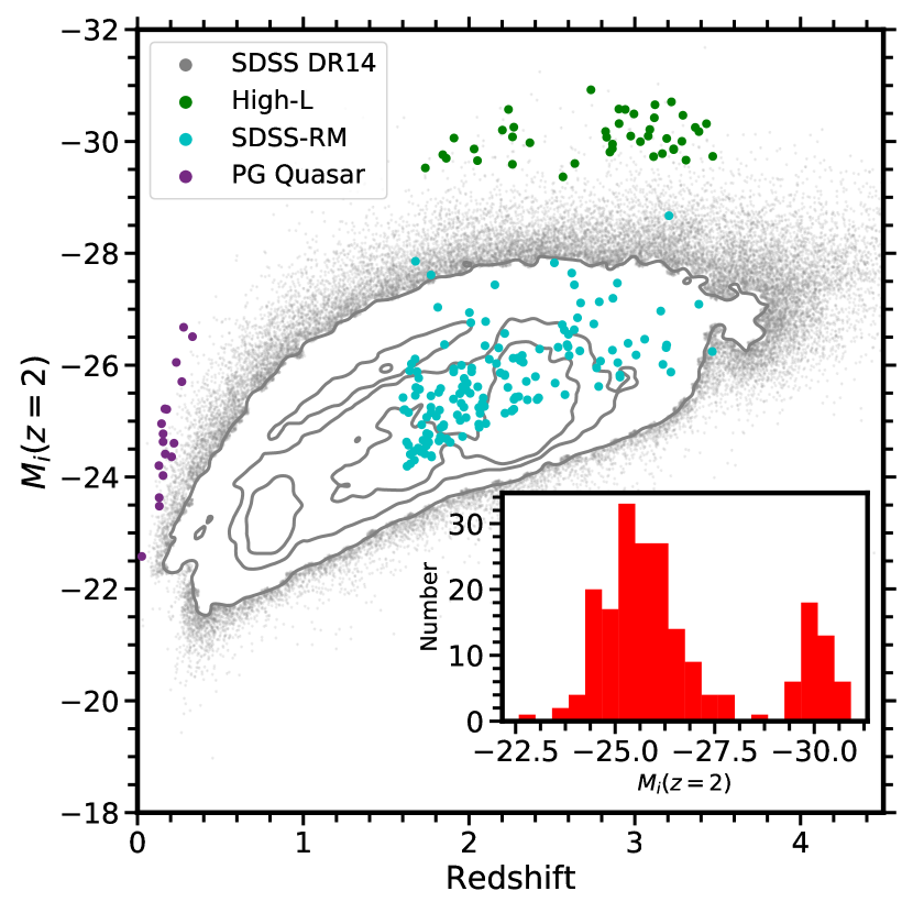
Figure 1: Absolute $i$-band magnitude (corrected to $z=2$; Richards et al. 2006) as a function of redshift for the High-$L$ (green), SDSS-RM (blue), and PG (purple) quasars. For reference, the SDSS DR14 quasars (Pâris et al., 2018) are depicted as grey contours that enclose 35, 68, and 95 percent of the data. The inset plot shows the $M_{i}(z=2)$ distribution of all of the quasars used to measure  He ii EW. The quasars in this sample span a wide range in luminosity at high-$z$, and a wide range in $z$ at low-luminosity, thus allowing us to separate the luminosity and redshift dependences explored here.

Table 1: Summary of quasar samples

Sample	$N_{\rm Q}$	$f_{\rm detected}^{\rm\,\text{He\,{ii}}}$	$f_{\rm detected}^{\mathrm{X-ray}}$	$\langle z\rangle$	$\langle M_{i}(z=2)\rangle$
(1)	(2)	(3)	(4)	(5)	(6)
High-$L$	43	0.907	0.860	2.79	$-$30.07
SDSS-RM	146	0.883	1.000	2.18	$-$25.73
PG	17	1.000	1.000	0.18	$-$24.77
Total	206	0.898	0.971	–	–

Notes: Basic properties of the High-$L$, SDSS-RM, and PG quasar samples. Column (2) reports the number of quasars in each sample, and the  He ii emission-line and  X-ray detection fraction are reported in columns (3) and (4). Columns (5) and (6) present the average redshift and absolute magnitude of each sample. The total number of quasars used to measure correlations is reported in the last row.

2.2 SDSS Reverberation-Mapping Quasars

Another sample of quasars used in this investigation is from the public data archive of the SDSS Reverberation-Mapping Project (SDSS-RM; Shen et al. 2015). SDSS-RM was designed to monitor 849 quasars in a $\approx 7$ deg² field over numerous epochs with the primary goal of measuring time lags between variations in the continuum flux and emission-line flux. SDSS-RM began measuring quasar spectra in 2014 and has been taking data through 2021, accumulating more than 75 spectral epochs of observations. These quasars span a wide range in redshift ($0.1\leq z\leq 4.5$) and luminosity. Recently, Shen et al. (2019) stacked 32 spectral epochs available through 2014 and publicly released these combined spectra as well as measurements of the continuum and emission-line properties. These high-quality stacked spectra generally have sufficient signal-to-noise to measure robustly even weak lines like the  He ii emission line. To include these quasars in our work, the redshift range was restricted as before for the High-$L$ quasars ($1.6\leq z\leq 3.5$) but their typical luminosity is $\approx 100$ times lower (see Table 1). Quasars that host BALs in their spectra, as well as radio-loud quasars, were also removed from the sample. Additionally, a magnitude limit of $i\leq 21$ was imposed on these quasars to increase the likelihood that the quasar spectrum had sufficient signal-to-noise to measure the  He ii emission-line properties. After these cuts were imposed, 146 SDSS-RM quasars remained in the sample. Figure 1 depicts their absolute magnitude as a function of redshift (blue points), and we report the basic sample properties in Table 1. We used the observed flux density at rest-frame 2500 Å from the Shen et al. (2019) catalog to compute $L_{2500}$ for these quasars.

The SDSS-RM field has also been covered by  X-ray observations with XMM-Newton, and  X-ray source catalogs are presented in Liu et al. (2020). The XMM-Newton observations were performed from 2016–2017 and overlap with 6.13 deg² of the SDSS-RM field. The source catalogs were generated using only the  X-ray survey, as opposed to performing forced photometry at the SDSS-RM target positions. We then matched these  X-ray catalogs to the 849 SDSS-RM quasars. All 146 SDSS-RM quasars that satisfy the sample restrictions above are detected in the soft  X-ray band in the Liu et al. (2020) catalog (observed frame 0.5–2 keV). Given the median redshift of these 146 quasars ($z=2.05$), the typical rest-frame band-pass covered by the soft  X-ray band is 1.52–6.12 keV, and it thus probes rest-frame 2 keV. The reported monochromatic 2 keV flux densities and luminosities, as well as the measurement uncertainties, were adopted for our investigation. As for the High-$L$ sample, we add to the measurement errors an additional 36% uncertainty in $L_{\rm 2keV}$ to account for  X-ray variability, and we conservatively adopt the 20% uncertainty to account for variability of $L_{2500}$.

2.3 Palomar-Green Quasars

The Palomar-Green (PG; Schmidt & Green 1983) quasar sample consists of low-to-moderate luminosity, blue type-1 quasars from the PG catalog (Green et al., 1986), many of which reside at lower redshift ($z<0.5$; e.g. Boroson & Green 1992). Additionally, Laor & Brandt (2002) gathered 56 PG quasars that had high-quality spectral observations of the rest-frame UV/optical from the Hubble Space Telescope archive and published their reduced spectra. In their sample, 35 PG quasars have coverage of the  He ii emission-line region and the surrounding continuum needed for fitting (1420–1710 Å; see Section 3). Five of these 35 PG quasars were flagged as radio-loud (Kellermann et al., 1994) and seven were flagged as either UV absorbed or exhibited a BAL or a miniBAL in the spectrum (e.g. Brandt et al. 2000). These quasars were removed from our sample leaving 23 quasars in the PG sample. To obtain the 2500 Å luminosity for the PG quasars, we converted the observed flux at rest-frame 3000 Å from Neugebauer et al. (1987) to rest-frame $L_{2500}$, assuming a spectral slope of $\alpha_{\nu}=-1$ in this spectral region. The measurement uncertainties of $L_{2500}$ for the PG quasars are generally insignificant compared to the 20% uncertainty we adopt to account for quasar UV continuum variability.

The PG quasars occupy a significantly lower region in redshift than the quasars in the High-$L$ and SDSS-RM samples, but a similar range of luminosities to the SDSS-RM sample. The low redshift (median $z=0.165$) implies that measurements of the hard  X-ray emission (2–10 keV in the observed frame) are required to probe similar rest-frame  X-ray energies (2.33–11.65 keV) to those used for the other samples. Of the 23 non-BAL, radio-quiet PG quasars, 17 have reported  X-ray coverage in the 4XMM catalog (Webb et al., 2020) or in small-sample archival work (Kaspi et al. 2005; Piconcelli et al. 2005; Inoue et al. 2007; Bianchi et al. 2009). In cases where there were multiple hard  X-ray observations of a PG quasar, we adopted the earliest observation, to be closest in time to the optical measurement of Neugebauer et al. (1987) used to measure the rest-frame 3000 Å luminosity (repeated observations are available for only three PG quasars).  X-ray measurement uncertainties were adopted from the  X-ray catalog that we used to obtain the 2–10 keV flux, and we again incorporate an additional 36% uncertainty on $L_{\rm 2keV}$ to account for  X-ray variability. Uncertainties in $\alpha_{\rm{ox}}$ are again computed using standard propagation of error. The absolute $i$-band magnitude as a function of redshift for the 17 PG quasars used in this work is depicted in Figure 1 (purple points).

2.4 The  He ii Sample

The full sample used in this work was generated by combining the 43 High-$L$, 146 SDSS-RM, and 17 PG quasars, which yields a total of 206 quasars (hereafter, the  He ii sample) that span wide ranges in luminosity and redshift. The High-$L$ and SDSS-RM samples allow us to probe luminosity dependence, independent of redshift, while the SDSS-RM and PG samples allow us to probe redshift dependence, independent of luminosity. All samples have corresponding high-quality spectra from which the  He ii EW can be measured. The full catalog of the 206 quasars used in this work is available in machine-readable format as documented in Appendix A.

3 Measuring the  He ii EW

The weak UV  He ii emission line peaks at a vacuum wavelength of $\lambda\approx 1640$ Å and is surrounded by C iv1549Å on the blue side and O iii]1663Å at redder wavelengths. Fitting the line profile of  He ii can be complicated if the spectrum has low signal-to-noise due to the fact that this line is both weak and is in close proximity to these other broad emission lines; however, the quasars in our sample were specifically selected due to their high-quality spectra to mitigate this problem. Moreover, a simpler method of systematically measuring the EW of this line was implemented in our work to avoid uncertainties that might arise due to model fitting of the blended emission-line profiles in this spectral region. The method used in our work is similar to that in Baskin et al. (2013) in which the  He ii EW was used as a measure of the ionizing SED hardness.

In our investigation, the local continuum in the  He ii emission-line region of each spectrum was determined by fitting a linear model to the median values in the continuum windows 1420–1460 Å and 1680–1700 Å. These windows are considered to be relatively free of broad emission-line features, and the quasars investigated in this work are devoid of BALs; therefore, the median fluxes in these windows are generally a good estimate of the local continuum flux. A $3\sigma$ clipping method was also incorporated when determining the median value in order to remove the effects of any narrow spikes in these regions. The  He ii EW was then measured by integrating directly the continuum-normalized flux in the window 1620–1650 Å. This wavelength range represents the location in the spectrum where the  He ii emission maximally contributes to the spectral flux above the red tail of the C iv emission line and is sufficiently blue-ward of any significant contribution from O iii] (Baskin et al., 2013). While this method does not capture the full line EW (recovering $\approx 90$% compared to model fitting), it measures the emission where  He ii dominates the spectrum. A key advantage of this method is that the  He ii emission is systematically measured, so any excluded emission from the tails of the line from the EW calculation is systematically excluded, and thus our results robustly recover the differences in the line emission between quasars with little bias.

Measurement uncertainties for the  He ii EW were determined using a Monte Carlo re-sampling routine with 1000 iterations. This Monte Carlo approach consisted of adding to the observed spectral flux a random value drawn from a normal distribution with mean zero and standard deviation equal to the spectral uncertainty. The spectra from Laor & Brandt (2002), however, did not provide the spectral uncertainty per pixel for the PG quasars; therefore, we adopted the standard deviation of the flux in the continuum regions as the spectral uncertainty per pixel. To remain consistent in our analysis of the quasar spectra, this spectral uncertainty was also used for both the PG and SDSS spectra. The  He ii EW was computed, as before, for each re-sampled emission line, and the standard deviation of all 1000 iterations was adopted as the $1\sigma$ measurement uncertainty of the  He ii EW. In addition to this uncertainty for each quasar, we also incorporated a 10% uncertainty due to variability in the line emission. We adopted this additional uncertainty value based on the investigation of Rivera et al. (2020), who measured variability of the C iv emission line in the SDSS-RM quasars, and found typical variability of the C iv EW of $\approx$10%.

As mentioned before, the  He ii line is a weaker broad emission line and thus, on occasion, it cannot be detected above the continuum, even in the high-quality spectra utilized in this investigation. A threshold for line detection was therefore determined and, in cases where the emission line was not detected, an upper limit on the emission-line flux was generated in order to compute upper limits on the  He ii EW. The detection threshold was set using the $p(\chi^{2},\nu)$ probability commonly employed in  X-ray astronomy to determine the quality-of-fit of a model to a set of data. This probability estimates the likelihood of the model fit using the $\chi^{2}$ statistic and the number of degrees of freedom, $\nu$. In this work, the model is considered to be the continuum fit, and the data that are being fit is the spectral measurement in the  He ii window 1620–1650 Å. We consider the  He ii emission line to be detected if $p(\chi^{2},\nu)\leq 0.001$ (i.e. if the likelihood that the continuum is a reasonable fit to the data is less than $0.1\%$). The  He ii emission-line detection fraction for each individual sample in Section 2, as well as for the entire  He ii sample, is reported in Table 1.

If the  He ii emission line is not detected significantly above the continuum level, an upper limit on the  He ii EW was estimated using a $\Delta\chi^{2}$ metric (e.g. Filiz Ak et al. 2012). To implement this method, we first calculated a reference chi-square value, $\chi^{2}_{\rm ref}$, between the continuum model and the measured flux in the  He ii emission-line region. Then the measured flux in the 1620–1650 Å window is increased uniformly by a constant value, and an updated chi-square value, $\chi^{2}_{\rm updated}$, was calculated using the new flux and the continuum model. The difference $\Delta\chi^{2}=\chi^{2}_{\rm updated}-\chi^{2}_{\rm ref}$ was computed and the above process repeated until $\Delta\chi^{2}=6.8$, which corresponds to a 99% confidence upper limit (e.g. Press et al. 1993). The  He ii EW was then computed, as before, by integrating under the updated emission line that satisfied the $\Delta\chi^{2}$ threshold.

4 Correlations

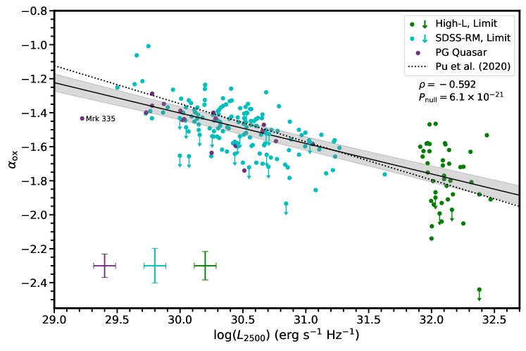
Figure 2: Optical-to-X-ray spectral slope, $\alpha_{\rm{ox}}$, as a function of 2500 Å luminosity for the PG (purple), SDSS-RM (blue), and High-$L$ (green) quasars in our sample. In cases where the quasar is not  X-ray detected (downwards arrows) the 90% confidence upper limit on $\alpha_{\rm{ox}}$ is reported. Median error bars are shown in the lower left-hand corner of this panel. The solid black line depicts the best-fit relationship to our data using the Kelly (2007) method and the grey shaded region encloses the $1\sigma$ confidence interval. This fitted relationship is largely consistent with the best-fit relationship from Pu et al. (2020) (black dotted line). The test statistic, $\rho$, and $p$-value from the Spearman rank-order test are reported in the top-right corner (see also Table 2). The location of the low-luminosity quasar Mrk 335 is highlighted since this quasar is known to be extremely  X-ray variable; therefore, the value of $\alpha_{\rm{ox}}$ is also likely highly variable.

The primary aim of this work is to investigate the relationships between $\alpha_{\rm{ox}}$,  He ii EW, and $L_{2500}$. These parameters of interest describe, for each quasar, the nature of the quasar ionizing SED. For  X-ray unabsorbed quasars, $\alpha_{\rm{ox}}$ is often used as a direct observational probe of the hardness of the ionizing SED in the quasar. It has been previously shown that there exists an anti-correlation between $\alpha_{\rm{ox}}$ and $L_{2500}$ (e.g., Steffen et al. 2006; Just et al. 2007; Lusso & Risaliti 2016; Timlin et al. 2020a; Pu et al. 2020) indicating that ionizing radiation is less abundant for more luminous quasars. The  He ii EW is a more direct indicator of the strength of the ionizing radiation that interacts with the quasar broad emission-line region (see Section 1). Previous investigations have demonstrated that the  He ii EW exhibits a strong Baldwin effect having one of the strongest anti-correlations with $L_{2500}$ of any broad emission line (e.g. Zheng & Malkan 1993; Laor et al. 1995; Green 1996; Korista et al. 1998; Dietrich et al. 2002). The following investigation seeks to determine whether a real and significant relation exists between $\alpha_{\rm{ox}}$ and  He ii EW, both of which are proxies of the strength of the ionizing SED in quasars, independent of their individual relationships with $L_{2500}$.

Table 2: Statistical tests for correlations and of similarity in each parameter space

				Spearman rank-order		Kendall Partial $\tau$
Parameter space	Slope ($\sigma_{\rm slope}$)	Intercept ($\sigma_{\rm intercept}$)	$\sigma_{i}(\sigma)$	$\rho\ (\sigma_{\rho})$	$P_{\rm null}^{\rho}$	$\tau\ (\sigma_{\tau})$	$P_{\rm null}^{\tau}$
(1)	(2)	(3)	(4)	(5)	(6)	(7)	(8)
$\alpha_{\rm{ox}}$–$L_{2500}$	$-$0.179(0.013)	3.968(0.423)	0.112(0.048)	$-$0.592(0.029)	$6.1\times 10^{-21}$	–a	–
He ii EW–$L_{2500}$	$-$0.306(0.021)	10.038(0.647)	0.180(0.068)	$-$0.637(0.026)	$4.2\times 10^{-24}$	–	–
$\alpha_{\rm{ox}}$– He ii EW	0.557(0.039)	$-$1.892(0.027)	0.080(0.044)	0.558(0.036)	$2.9\times 10^{-18}$	–	–
$\Delta\alpha_{\rm{ox}}$–$L_{2500}$	0.017(0.013)	0.537(0.406)	0.110(0.046)	$-$0.115(0.043)	$9.9\times 10^{-2}$	–	–
$\Delta\alpha_{\rm{ox}}$– He ii EW	0.187(0.037)	$-$0.115(0.026)	0.099(0.045)	$-$0.207(0.047)	$2.9\times 10^{-3}$	–	–
$\Delta\alpha_{\rm{ox}}$–$\Delta$ He ii EW	0.462(0.060)	$-$0.003(0.009)	0.074(0.040)	0.285(0.050)	$3.3\times 10^{-5}$	0.332(0.039)	1.8$\times 10^{-15}$

Notes: Best-fit parameters and correlation statistics for each parameter space in this work. Columns (2)–(4) report the slope, intercept, and intrinsic dispersion along with their $1\sigma$ uncertainties (in parentheses) measured using the method of Kelly (2007). Furthermore, the correlation coefficient (and $1\sigma$ uncertainty) and $p$-value of the Spearman rank-order test are presented in columns (5)–(6). Uncertainties in the test statistic were computed using a Monte Carlo method (e.g. see Timlin et al. 2020a). Columns (7)–(8) report the test statistic (and $1\sigma$ uncertainty) and $p$-value of a Kendall partial $\tau$ test for the residual parameter spaces in the last two rows.
^a No partial correlations can be computed for these relationships since there are only two parameters of interest.

Figure 3: The Baldwin effect between log( He ii EW) and log($L_{2500}$) for the quasars in our sample. The color scheme is the same as in Figure 2, the black line and grey shaded region depict the best-fit line and the $1\sigma$ confidence interval derived using the method of Kelly (2007), and the median error bars are shown in the bottom-left corner. The downward-pointing arrows depict the upper limit of the  He ii EW when the emission line is not detected with 99% significance (see Section 3 for details). As is the case generally for quasar emission lines, a strong Baldwin effect exists in this parameter space according to a Spearman rank-order test (the $\rho$ and $p$-value reported in the upper right-hand corner).

4.1 The relationships between $\alpha_{\rm{ox}}$,  He ii EW, and $L_{2500}$

To assess the joint relationships between the three parameters of interest, we must first understand better the behavior of the data in their two-dimensional parameter spaces ($\alpha_{\rm{ox}}$–$L_{2500}$,  He ii EW–$L_{2500}$, and $\alpha_{\rm{ox}}$– He ii EW). Using the 206 quasars in the  He ii sample assembled in Section 2, we first investigated the dependence of $\alpha_{\rm{ox}}$ on $L_{2500}$, depicted in Figure 2. As mentioned above, there is a well-known anti-correlation between these two parameters with a slope between $\approx 0.14$–$0.22$ depending on the range of $L_{2500}$ probed and the properties of the quasars utilized in the investigation (e.g. whether the sample included or excluded potentially  X-ray absorbed quasars; e.g. Pu et al. 2020). Figure 2 depicts the $\alpha_{\rm{ox}}$–$L_{2500}$ parameter space for our sample of quasars from the High-$L$ (green points), SDSS-RM (blue points), and PG (purple points) samples. Quasars that were not detected in the  X-ray are marked by downward-pointing arrows, and are positioned at the location of the 90% confidence upper limit on $\alpha_{\rm{ox}}$. Median error bars for each sample are depicted in the bottom left of Figure 2, where the uncertainties are the quadrature sum of both measurement uncertainties and the uncertainties due to variability.

A Spearman rank-order correlation test was used to determine the significance of the visually apparent anti-correlation in these data; however, this test is not suitable for censored data. To incorporate the censored data points (in this case, the  X-ray upper limits) into the test, we randomly re-sampled their values from the probability density function (PDF) of the corresponding data set (i.e. upper limits in the High-$L$ sample were redrawn from the PDF of the High-$L$ sample only), and the maximum value allowed to be drawn is set at the upper-limit value. In cases where the upper-limit value is smaller than all of the detections in the sample, the re-sampled value is drawn from a uniform distribution between the limit value and the limit value minus the sample’s median $1\sigma$ measurement uncertainty. This upper-limit resampling was performed 100 times, and the median test statistic, $\rho$, and corresponding $p$-value of the Spearman test are reported in Table 2. The resulting test statistic ($\rho=-0.592$) and corresponding probability ($p=6.1\times 10^{-21}$) that the correlation happens by chance clearly indicate that there is a significant anti-correlation between $\alpha_{\rm{ox}}$ and $L_{2500}$ in this data set. Also reported in Table 2 is the $1\sigma$ uncertainty value of the test statistic which was estimated using 1000 Monte Carlo re-sampling iterations.

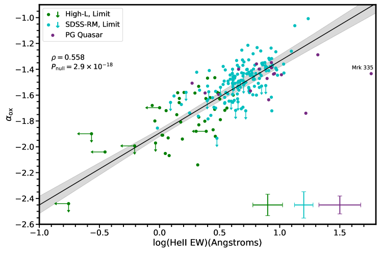
Figure 4: Dependence of $\alpha_{\rm{ox}}$ on log( He ii EW) for our sample along with the best-fit line and $1\sigma$ confidence interval (color schemes are the same as in Figure 2). Left-pointing arrows depict upper limits in the measurement of the  He ii EW, and downward-pointing arrows depict the 90% confidence upper limit of $\alpha_{\rm{ox}}$ for  X-ray non-detections. A significant relationship exists according to a Spearman rank-order test (statistics reported in the top left corner). The three correlations presented in Figures 2–4 are measured to be similarly strong (see Table 2).

Since a significant anti-correlation exists, a relationship was fitted between these two parameters using the method from Kelly (2007), as implemented in the linmix Python package. This implementation utilizes a hierarchical Bayesian model to fit a univariate model to data, incorporates errors in both the x- and y-dimensions, and can model censored data in the dependent variable. The best-fit slope ($\beta$) and intercept ($\alpha$) are output as well as an estimate of the intrinsic scatter ($\sigma_{\epsilon}$) around the regression line. This code also reports the $1\sigma$ uncertainty in the fitted parameters and returns the confidence interval of the fit (in this work, we report the $1\sigma$ confidence interval, unless otherwise noted). We depict the best-fit model in Figure 2 as the solid black line, and the confidence interval as the grey shaded region. The slope and intercept of the fitted model are $\beta=-0.179\pm 0.013$ and $\alpha=3.968\pm 0.423$, respectively, and the standard deviation of the intrinsic scatter is $\sigma_{\epsilon}=0.112\pm 0.048$ (see Table 2). This fitted relationship is consistent with other values found in the literature (e.g. Steffen et al. 2006; Just et al. 2007; Timlin et al. 2020a); however, it is slightly flatter than that found most recently in Pu et al. (2020) (dashed line in Figure 2), which removed  X-ray absorbed quasars from their analysis. The consistency of this result with those in the literature further confirms that the quasar sample in this work is representative of the general quasar population.

Next, we investigated the Baldwin effect of the  He ii EW for the quasars in the  He ii sample. Previous investigations have investigated the  He ii Baldwin effect for either small samples or using stacked spectra (see references at the beginning of this Section). Our investigation, on the other hand, is the first large-scale investigation of the  He ii Baldwin effect for individual quasars, allowing us also to assess the amount of scatter present in the relationship. Depicted in Figure 3 is the  He ii EW as a function of $L_{2500}$ separated by the three sub-samples in Section 2, using the same color scheme as in Figure 2. A Spearman rank-order test was performed as described above to determine the strength of the observed anti-correlation in this parameter space. As has been found in previous investigations, a significant anti-correlation exists between  He ii EW and $L_{2500}$ (see Table 2 for the values and uncertainty measurements). The solid-black line and grey-shaded region in Figure 3 again depict the best-fit linear model to the data and the $1\sigma$ confidence interval, respectively, fitted using the method from Kelly (2007). The best-fit slope from our data ($\beta=-0.306\pm 0.021$) is slightly larger than what has been found in previous investigations (most recently from Dietrich et al. 2002 who found $\beta=-0.20\pm 0.04$ using a similarly wide range of luminosity as our investigation). This small difference between the slopes can likely be attributed to the small  He ii EW outliers in the High-$L$ sub-sample which steepen the slope of our fitted relationship (see the green arrows in Figure 3). Additionally, Dietrich et al. (2002) ignore their highest luminosity bin when fitting the Baldwin relationship for their data which effectively flattens the fitted slope (see Figure 7 of Dietrich et al. 2002). We report the intrinsic scatter of our data in Table 2. Despite this mild difference in slope, the data gathered in this investigation recover the strong  He ii Baldwin effect.

The last two-dimensional parameter space evaluated in this work is the $\alpha_{\rm{ox}}$– He ii EW space presented in Figure 4, again using the same symbols and color schemes as in Figure 2. A strong correlation is found between $\alpha_{\rm{ox}}$ and  He ii EW (see Table 2 for the Spearman-test results) and thus we again fitted a linear relation to the data in this parameter space. The regression method from Kelly (2007), however, is not designed to handle censored data as the independent variable; therefore, we accounted for the six  He ii EW upper limits by re-sampling the  He ii EW values as was described previously for the Spearman correlation test. Upper limit re-sampling was performed 100 times, with each iteration being fitted separately, resulting in a distribution of best-fit parameters. The fit that produced the median slope ($\beta=0.557\pm 0.039$; see Table 2) was adopted as the best-fit relationship, and is depicted as the black line in Figure 4 (the grey shaded region depicts the corresponding $1\sigma$ confidence interval).

As depicted in Figures 2–4, the SDSS-RM and PG quasars, which have similar luminosity yet largely different redshift (see Table 1), overlap in all three parameter spaces indicating that the correlations presented here are independent of redshift.

A comparison of the three Spearman $\rho$ values from Table 2 for the two-dimensional parameter spaces discussed above suggests that the correlations are all comparable in strength. This similarity of these correlations suggests that there is an interdependence between $\alpha_{\rm{ox}}$,  He ii EW, and $L_{2500}$ that cannot be untangled through investigation of these two-dimensional parameter spaces alone. A reasonable question that we wish to address in the following sub-section is to what degree do two of these relationships impact the third? For example, both $\alpha_{\rm{ox}}$ and  He ii EW are clearly strongly related to $L_{2500}$, but do the $\alpha_{\rm{ox}}$–$L_{2500}$ and  He ii EW–$L_{2500}$ correlations drive the $\alpha_{\rm{ox}}$– He ii EW relationship, or is there an $\alpha_{\rm{ox}}$– He ii EW relationship independent of $L_{2500}$? Moreover, if the relationships with $L_{2500}$ drive the $\alpha_{\rm{ox}}$– He ii EW relationship, is one of the $L_{2500}$ relationships dominant and the other simply a secondary effect? Below, we jointly analyze all three parameters to understand better how they are related.

4.2 The interdependence of $\alpha_{\rm{ox}}$, $L_{2500}$, and  He ii EW

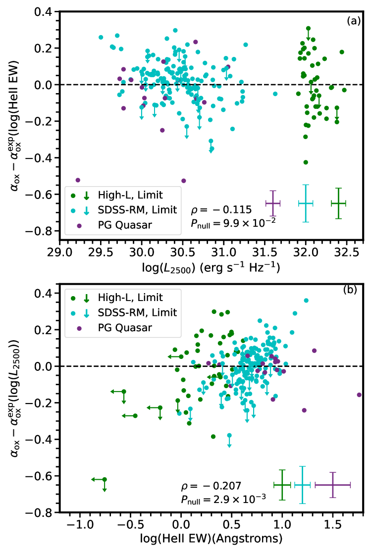
Figure 5: Panel (a): Residual relationship between $\alpha_{\rm{ox}}$ and log₁₀($L_{2500}$), accounting for the dependence of $\alpha_{\rm{ox}}$ on log₁₀( He ii EW). Panel (b): Residual relationship between $\alpha_{\rm{ox}}$ and log₁₀( He ii EW), accounting for the dependence of $\alpha_{\rm{ox}}$ on log₁₀($L_{2500}$). The left-pointing arrows in this panel depict the quasars that have upper limits on their measured  He ii EW, and the horizontal dashed line represents zero residual. The color scheme and symbols are the same as in Figure 2. In both panels, the Spearman rank-order correlation suggests that, if a correlation exists, it is not highly significant (see Table 2). The apparent lack of correlation in these residual parameter spaces, along with the significance of the coefficients in the bivariate regression in Figure 7 suggests that these three parameters might be intrinsically related.

To assess the interdependence of the three parameters of interest, we first investigated residual relationships. In particular, we first examined the residual relationship between the measured $\alpha_{\rm{ox}}$ and the expected $\alpha_{\rm{ox}}$ calculated from the relationships shown in Figures 2 and 4 (we denote the residual as $\Delta\alpha_{\rm ox}$). We then investigated the correlation of $\Delta\alpha_{\rm ox}$ with respect to the parameter not used to compute the residual. For example, in Figure 5 panel (a), we depict the residual between $\alpha_{\rm{ox}}$ and the $\alpha_{\rm{ox}}$ expected from the $\alpha_{\rm{ox}}$– He ii EW relationship (Figure 4) as a function of $L_{2500}$. A Spearman rank-order test performed on the data in this space returns a small correlation coefficient ($\rho=-0.115$, see Table 2), which indicates that, if a correlation between $\Delta\alpha_{\rm ox}$ and $L_{2500}$ exists, it is weak. Similarly, Figure 5 panel (b) depicts the residual space with $\Delta\alpha_{\rm ox}$ now being computed between $\alpha_{\rm{ox}}$ and that expected from the $\alpha_{\rm{ox}}$–$L_{2500}$ (Figure 2) relation and depicted as a function of  He ii EW. As in the previous case, a Spearman correlation test indicates a potentially mild relationship, if one exists at all ($\rho=-0.207$, see Table 2). The similarity of the correlations for the data in both panels of Figure 5 suggests that the relationships in Figures 2–3 are not dominated by a single parameter space. Furthermore, the correlations of the data in Figure 5 (and Table 2) indicate that $\alpha_{\rm{ox}}$ correlates as strongly with  He ii EW as it does with $L_{2500}$, if not slightly more so, which is a notable result given that previous investigations have been unable to find another parameter that correlates as strongly with $\alpha_{\rm{ox}}$ as $L_{2500}$ (e.g. Shemmer et al. 2008; Liu et al. 2021).

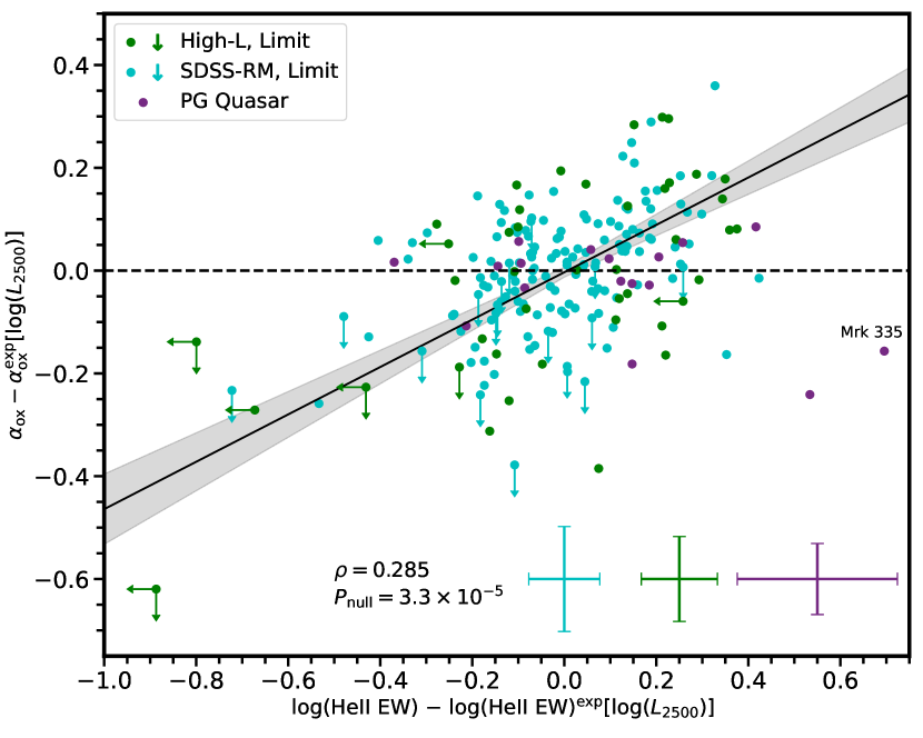
Figure 6: Residual relationship between $\alpha_{\rm{ox}}$ and  He ii EW accounting for both of their dependences on $L_{2500}$. Unlike both panels in Figure 5, a significant correlation exists in this parameter space (see Table 2) according to a Spearman test, and thus a relationship was fitted (black solid line) along with the $1\sigma$ confidence interval (grey shaded region). A Kendall partial $\tau$ test further indicates that a correlation exists in this residual space ($\tau=0.332\pm 0.039$, $p$-value $=1.8\times 10^{-15}$). The positive correlation between these residuals further demonstrates the existence of a fundamental relationship between $\alpha_{\rm{ox}}$ and  He ii EW after normalizing for their $L_{2500}$ dependence. This, in turn, indicates that an additional factor, along with the quasar luminosity, is responsible for setting the ionizing continuum in the quasar.

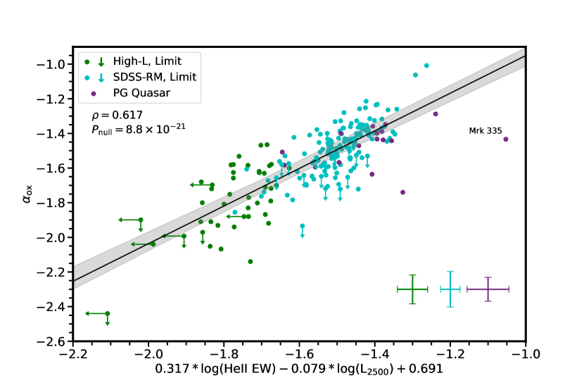
Figure 7: Bivariate regression of $\alpha_{\rm{ox}}$ as a function of both log( He ii EW) and log($L_{2500}$) for the quasars in our sample (the colors and symbols are the same as in Figure 2). A strong correlation exists according to the Spearman rank-order test ($\rho$ and the $p$-value are reported in the top left). Furthermore, the coefficients of both log( He ii EW) and log($L_{2500}$) are statistically different from zero ($7.9\sigma$ and $4.6\sigma$, respectively; see Equation 2), suggesting that both parameters are significantly related to the strength of the ionizing continuum rather than one being a primary and the other only a secondary factor.

With no single parameter space dominating the relationships in Figures 2–4, we next investigated whether a correlation between two parameters exists after removing the contribution of the third parameter. Investigating the correlation between $\alpha_{\rm{ox}}$ and  He ii EW, after accounting for their dependence on $L_{2500}$, is of particular interest in this investigation since these are the probes of the ionizing continuum strength. Figure 5 panel (b), in which we already accounted for the luminosity dependence of $\alpha_{\rm{ox}}$, shows a stratification of the High-$L$, RM, and PG quasars which is likely the result of the dependence of  He ii EW on $L_{2500}$. To investigate this further, we computed $\Delta$ He ii EW by removing the luminosity dependence from the  He ii EW using the relationship presented in Figure 3 and the $L_{2500}$ value. We depict the $\Delta$$\alpha_{\rm{ox}}$–$\Delta$ He ii EW residual parameter space in Figure 6, using the same symbols and color scheme as in the previous figures. A Spearman rank-order test indicates that a significant correlation exists in this space; therefore, we fit a relationship to these data using the same method employed to fit the relationship in Figure 4 (see Table 2 for the results of the correlation test and the best-fit parameters).

We confirm the existence of a correlation in the residual space in Figure 6 using a Kendall’s partial $\tau$ test (e.g. see Akritas & Siebert 1996 and references therein). Kendall’s partial $\tau$ numerically tests for a correlation between two parameters after removing the contribution of their correlations with a third parameter. This test combines the Kendall rank-correlation statistic, $\tau_{12}$ (Kendall, 1938), with the Pearson partial product-moment correlation (Kendall, 1970) resulting in the equation

$$\tau_{12,3}=\frac{\tau_{12}-\tau_{13}\tau_{23}}{[(1-\tau_{13}^{2})(1-\tau_{23}^{2})]^{1/2}},$$ (1)

where $\tau_{12,3}$ is the partial correlation between parameter 1 and parameter 2, removing the effect of parameter 3. This test is also particularly useful for our investigation since it has been created to handle censored data (which are the upper limits in our case), and it has the capability to provide a significance level to the partial correlation. In our case, we compute $\tau_{\alpha_{\rm ox}{\rm EW},L_{2500}}$ which is the partial correlation between $\alpha_{\rm{ox}}$ and  He ii EW after removing the effect of $L_{2500}$. We find a partial-correlation strength of $\tau_{\alpha_{\rm ox}{\rm EW},L_{2500}}=0.332$ with a corresponding $p$-value of $1.8\times 10^{-15}$ (see the bottom row of Table 2), which indicates that a significant partial correlation exists in this space. The correlation in this space indicates that there is an intrinsic relationship between $\alpha_{\rm{ox}}$ and  He ii EW that is independent of luminosity. This, in turn, suggests that the X-rays and EUV continuum are coupled through another physical mechanism in addition to the UV luminosity.

The aforementioned tests are robust methods of determining the statistical significance of any residual correlations among the three parameters of interest. Another way to quantify the relationship is through an analysis of the fitting parameters in a bivariate regression. In this work, we fitted $\alpha_{\rm{ox}}$ as a function of both  He ii EW and $L_{2500}$ with a bivariate linear model and analyzed the significance, relative to zero, of the best-fit coefficients. The bivariate regression was performed using the emcee Python package (Foreman-Mackey et al., 2013). One advantage of using emcee for regression is that the uncertainties in all of the variables (in this case, 1 dependent and 2 independent variables) can be included in the regression; however, it does not handle censored data. In order to include the small fraction of upper limits in the fitting routine, we again performed resampling of the data 100 times using the methods outlined in the previous sub-section. The best-fit model was chosen to be the model corresponding to the median value of the  He ii EW coefficient. The best-fit equation of the model is the following:

$$\alpha_{\rm ox}={} (0.317\pm 0.040)\mathrm{log(\text{He\,{ii}}\ EW)}$$ (2)

$$-(0.079\pm 0.017)\mathrm{log}(L_{2500})+(0.691\pm 0.555),$$

$$\sigma_{\epsilon}=(0.086\pm 0.012).$$

Figure 7 depicts $\alpha_{\rm{ox}}$ as a function of the combination  He ii EW and $L_{2500}$ using the best-fit model in Equation 2. The solid black line in this figure depicts the $y=x$ line and the grey shaded region depicts the $1\sigma$ confidence interval (computed using the method of Kelly 2007). Comparing the coefficients in Equation 2, we find that  He ii EW and $L_{2500}$ are different from zero by $\approx 7.9\sigma$ and $\approx 4.6\sigma$, respectively, again indicating that both parameters contribute significantly in modeling $\alpha_{\rm{ox}}$. As before, this result may suggest that $\alpha_{\rm{ox}}$ is more dependent on  He ii EW than on $L_{2500}$; however, further investigation comparing these parameters is required before any definitive conclusion can be made.

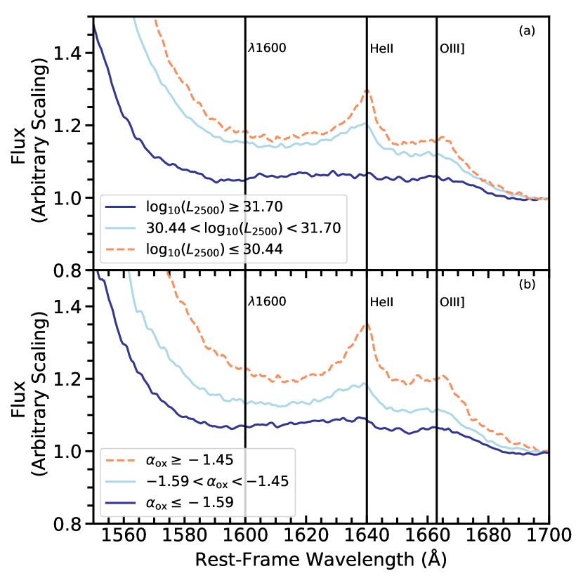
Figure 8: Median-stacked  He ii emission-line regions in three bins in ${\rm log}(L_{2500})$ (panel a) and $\alpha_{\rm ox}$ (panel b). As expected from Figure 3, the median  He ii emission-line profile of the low-luminosity bin (orange dashed line) in panel (a) is more prominent than both the intermediate-luminosity (light blue line) and high-luminosity (dark blue line) bins. In panel (b), the strength of the median-stacked  He ii emission-line profile decreases with decreasing $\alpha_{\rm ox}$ (orange dashed line, light blue line, and dark blue line, respectively) as expected from the relationship depicted in Figure 4.

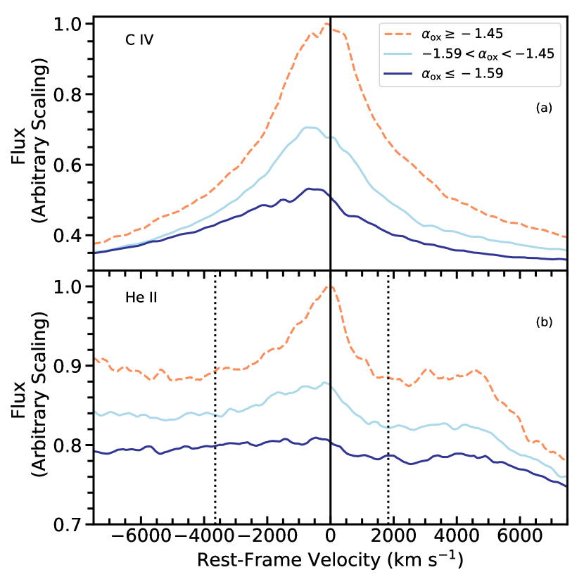
Figure 9: Median-stacked  C iv (panel a) and  He ii (panel b) emission lines in the three $\alpha_{\rm ox}$ bins from panel (b) of Figure 8. The solid vertical black lines in both panels depict the vacuum wavelength of the emission-line peaks. The vertical dotted lines in panel (b) depict the region in which the  He ii emission significantly contributes to the spectral emission, within which we computed the  He ii EW (1620–1650 Å; see Section 3). Both panels demonstrate that these emission lines become more blueshifted and increasingly asymmetric about the line center as $\alpha_{\rm ox}$ decreases. The growing asymmetry is seemingly stronger for the  He ii emission line within the dotted lines in panel (b) compared to the evolution seen in the  C iv emission line. Panel (b) also demonstrates that the  He ii emission line is significantly blended with its surroundings, which motivated our model-independent fitting method.

A visual comparison of the  He ii emission-line profiles of our quasars in bins of $L_{2500}$ and $\alpha_{\rm{ox}}$, depicted in Figure 8, also provides useful insights into changes of the  He ii emission line with these parameters. To generate panel (a) of Figure 8, we grouped the data first in three bins of $L_{2500}$, where we separated the high-$L$ from the SDSS-RM and PG quasars as one bin, and then split the SDSS-RM and PG by their median $L_{2500}$ ($\rm{log}$($L_{2500}$) = 30.44) to generate the other two lower luminosity bins. Stacking was performed using the cleaned spectra (i.e. corrected for Galactic extinction and $3\sigma$ clipped to remove spurious outliers) by projecting the individual spectra in each bin onto a common frame, normalized to the median flux value in the range 1700–1705 Å. The spectra depicted in panel (a) of Figure 8 show the median pixel value of all of the individual spectra within the respective bin. In total, the highest luminosity bin (dark blue) is a stack of 43 spectra, the middle-luminosity bin (light blue) depicts 81 stacked spectra, and the low-luminosity bin (orange dashed) depicts 82 stacked spectra. The spectra in panel (b) are produced in the same manner; however we binned by $\alpha_{\rm{ox}}$, splitting the range of $\alpha_{\rm{ox}}$ into three, nearly equally-sized bins. The large $\alpha_{\rm{ox}}$ bin (orange dashed) contains 70 spectra, the middle bin in $\alpha_{\rm{ox}}$ (light blue) contains 68 spectra, and the small $\alpha_{\rm{ox}}$ bin (dark blue) also contains 68 spectra. Both panels in Figure 8 depict the expected behavior of the  He ii emission line, with the low-$L$ bin (and high $\alpha_{\rm{ox}}$ bin) displaying the largest  He ii EW whereas the high-$L$ bin (and small $\alpha_{\rm{ox}}$ bin) show weak  He ii emission.

We also observe that the  He ii emission line is highly asymmetric, and appears to become more asymmetric moving from strong to weak  He ii emission, with a blue wing extending as far as $\approx 1590$ Å (corresponding to $\approx 9000$ km s^-1) at the highest luminosity and steepest $\alpha_{\rm{ox}}$ bins. Similar behavior is often observed for the  C iv emission line as demonstrated in Figure 11 of Timlin et al. (2020a) where quasars with weaker  C iv emission lines also tend to have more asymmetric and blueshifted line profiles. A visualization of the stacked  C iv and  He ii emission-line profiles for our sample as a function of $\alpha_{\rm{ox}}$ is depicted in Figure 9. The  He ii emission line rapidly becomes asymmetric with decreasing $\alpha_{\rm{ox}}$ within the region where it contributes significantly to the spectral emission (i.e. within the dotted lines in panel (b) of Figure 9). Also, as $\alpha_{\rm{ox}}$ decreases the line peaks of  C iv and  He ii appear to be increasingly blueshifted (see Figure 1 in Shen et al. 2016 for a comparison of the relative line shifts between these lines). Finally, we performed a stacked spectral analysis to assess whether there was a redshift dependence of the  He ii EW by comparing the spectral profiles of the PG and RM quasars since they span a similar luminosity range but are at different redshifts. Our data suggest that there is no redshift dependence, where the median  He ii EW value for the PG quasars (log( He ii EW) $=0.91\pm 0.34$) is statistically consistent with that of the RM quasars (log( He ii EW) $=0.70\pm 0.20$).

5 Discussion

5.1 Results from earlier related investigations

Detailed investigations of proxies of the strength of the ionizing EUV continuum have been critically important to modeling and understanding better the physical properties of quasars. For example, the  C iv emission line has been shown to exhibit a blueshift with respect to the systemic redshift, which has been used in the literature as observational evidence for a disk-wind model of quasar outflows (e.g. Richards et al. 2011 and references therein). Analyses of the  C iv EW– C iv blueshift parameter space have demonstrated that quasars with large  C iv EW (EW $\geq$ 50 Å) generally exhibit modest blueshift whereas those with smaller  C iv EW (EW $\leq$ 15 Å) can exhibit very high-velocity outflows ($v>4000$ km s^-1; e.g. Wu et al. 2011; Luo et al. 2015). In the context of this model, the disparity in the outflow velocity is partly the result of the quasar wind region being over-ionized (in the case of high  C iv EW), and thus the less-energetic UV line driving in this component is inefficient (e.g. Leighly 2004; Richards et al. 2011); however, when the number of ionizing photons in the wind region is small, perhaps due to disk geometry (e.g. Leighly 2004; Luo et al. 2015), the line driving becomes more efficient.

Both $\alpha_{\rm{ox}}$ and  He ii EW have been studied independently to determine their distribution within the  C iv EW– C iv blueshift parameter space and to investigate their relationship with outflow velocity. Investigations of the distribution of $\alpha_{\rm{ox}}$ in the  C iv EW– C iv blueshift parameter space generally show harder (less negative) $\alpha_{\rm{ox}}$ values occupy the large  C iv EW, low  C iv blueshift region and softer (more negative) $\alpha_{\rm{ox}}$ values occupy the small  C iv EW, high  C iv blueshift space (e.g. Kruczek et al. 2011; Wu et al. 2011; Timlin et al. 2020a), albeit with significant scatter. Moreover, previous work has demonstrated that $\alpha_{\rm{ox}}$ is individually correlated with both the  C iv emission-line outflow velocity and  C iv EW (e.g. Vietri et al. 2018; Timlin et al. 2020a) further indicating that $\alpha_{\rm{ox}}$ is a good proxy of the balance between the strength of the ionizing SED and the line-driving radiation.

Despite the weakness of the  He ii emission line, previous investigations have gathered high-quality spectra with which to measure the  He ii EW so that it can be compared with  C iv emission-line and absorption-line properties. Baskin et al. (2013, 2015) found that the  He ii EW is related to both the profile and blueshift of the high-ionization broad absorption lines (BALs) in quasars, indicating that the  He ii EW is a good proxy of the outflow velocity. Recently, Rankine et al. (2020) investigated the behavior of the  He ii EW within the  C iv EW– C iv blueshift parameter space (see the left-hand panel of their Figure 12). They found that the average  He ii EW smoothly varies throughout the  C iv EW– C iv blueshift parameter space, with large  He ii EW values occupying the high  C iv EW, low  C iv blueshift region and small  He ii EW values occupying the small  C iv EW, large  C iv blueshift region of the parameter space. As is the case with $\alpha_{\rm{ox}}$, the relationships between the  He ii EW and the  C iv emission-line properties suggest that the  He ii EW is also a useful diagnostic to measure the amount of ionizing radiation and the line-driving efficiency of the less-energetic UV radiation.

The combination of the results from these previous investigations suggest that a correlation might exist between $\alpha_{\rm{ox}}$ and  He ii EW; however, no direct comparison has been made between these parameters until now.

5.2 Results of this work

In this work, we found a strong correlation between $\alpha_{\rm{ox}}$ and  He ii EW, both of which can therefore be used as proxies for the strength of the ionizing continuum of the quasar SED. Both of these parameters are also well known to be individually anti-correlated with $L_{2500}$ (see the references in Sections 1 and 4), and we depict these relationships for our data in Figures 2 and 3. Since both of these parameters exhibit such a strong anti-correlation with $L_{2500}$, we investigated whether or not the $\alpha_{\rm{ox}}$– He ii EW correlation is simply a secondary effect resulting from the combination of the $\alpha_{\rm{ox}}$–$L_{2500}$ and  He ii EW–$L_{2500}$ relationships. We found that a significant $\alpha_{\rm{ox}}$– He ii EW relationship remains after removing the effects of $L_{2500}$ (demonstrated in Figures 5–8 and by a partial-correlation test). The  He ii EW is therefore providing additional independent information into the nature of the ionizing SED in quasars.

It is not immediately apparent that there should be a strong correlation between $\alpha_{\rm{ox}}$ and  He ii EW since the ionizing radiation responsible for the production of  He ii is effectively independent of the harder  X-ray emission. To demonstrate this mathematically, we adopt a simple power-law to model the ionizing continuum at $\approx 50$ eV (near the ionization energy of  He ii) with an energy index of $\alpha_{\rm ion}=-1.6$ (e.g. Figure 5 in Baskin et al. 2014), corresponding to a photon index of $\Gamma_{\rm ion}=-2.6$. Integrating under this power-law indicates that the majority of the photons in the  He ii ionizing portion of the SED are largely outside of the soft  X-ray regime, where $\approx$ 90% of the photons lie within the energy range of 50 eV to 0.2 keV. The 2 keV  X-ray emission used to compute $\alpha_{\rm{ox}}$, therefore, should have little effect on the production of the  He ii ion. Moreover, the ionizing EUV photons are thought to be produced in the inner accretion-disk region (likely with some Comptonization; e.g. Petrucci et al. 2018 and references therein) whereas the harder  X-ray photons are generally thought to be produced in the corona above the disk. The tight correlation found in this work between $\alpha_{\rm{ox}}$ and  He ii EW therefore suggests that the production mechanism of the harder  X-ray photons is coupled to that of the EUV photons such that, when the mechanism changes, it affects the strengths of the  X-ray and EUV portions of the SED similarly.

The residuals in Figure 5 demonstrate that the negative correlations of both $\alpha_{\rm{ox}}$ and  He ii EW with $L_{2500}$ are significant and non-secondary relationships. The UV continuum is largely generated, in the standard model, by thermal emission from the quasar accretion disk which may not be significantly related to the (non-thermal) mechanism that produces the power-law ionizing EUV continuum. The relationships found in this work, however, suggest that there is a link between the thermal UV emission, the power-law EUV ionizing SED, and the  X-ray coronal properties in each quasar. In other words, it similarly impacts the strength of the quasar SED in the thermally dominated UV region, the power-law EUV region, and the  X-ray coronal region.

The residual $\alpha_{\rm{ox}}$– He ii EW relationship (after removing their $L_{2500}$ dependences) further demonstrates that these two parameters are related by an additional physical mechanism rather than only the UV luminosity. A physical property which may potentially affect the EUV disk emission, in addition to luminosity, is the gas metallicity. If the commonly observed continuum spectral break below 1000 Å (e.g. Lusso et al. 2015) is indeed due to radiation-pressure driven mass loss (Laor & Davis, 2014), then increased metallicity leads to a higher mass-loss rate, which lowers the inner accretion-disk temperature, and likely lowers the ionizing continuum. The increased disk mass loss, which inevitably passes through the coronal layers, may cool the coronal gas, and thus lower also the  X-ray emission.

As outlined in Section 1, the  He ii EW is expected to be more direct measure of the strength of the ionizing SED relative to the underlying UV continuum than the  C iv EW. To test this more directly, we compare the strengths of the individual correlations of  C iv and  He ii with $\alpha_{\rm{ox}}$. While multiple studies have investigated the $\alpha_{\rm{ox}}$– C iv EW relationship (e.g. Green 1998; Gibson et al. 2008; Kruczek et al. 2011; Timlin et al. 2020a), we can compare the results above directly with the previous work of Timlin et al. (2020a), in which the $\alpha_{\rm{ox}}$– C iv EW properties of 637 quasars were analyzed, since the analysis methods are nearly identical. We find both a stronger Spearman correlation coefficient and a significantly steeper best-fit slope in the $\alpha_{\rm{ox}}$– He ii EW parameter space ($\rho=0.558\pm 0.036,\beta=0.557\pm 0.039$, respectively; see Table 2) than in the $\alpha_{\rm{ox}}$– C iv EW parameter space ($\rho=0.470\pm 0.016,\beta=0.390\pm 0.027$, respectively; see Table 2 and Equation 4 in Timlin et al. 2020a). The differences between the strengths of these relationships reflects the scatter and apparent non-linearity in the relation between the  C iv EW and the  He ii EW (see Appendix C). The  C iv EW is only a secondary indicator of the ionizing continuum, compared to the  He ii EW, as it depends also on the environmental conditions (see Section 1). The relation between the  C iv EW and the  He ii EW derived in Appendix C can be used to estimate the  He ii EW in lower signal-to-noise spectra where only the  C iv EW is measurable.

Our investigation indicates that extreme variability of the ionizing EUV and  X-ray luminosities are not commonly observed. Our sample was constructed using quasars from multiple different samples that often had large temporal gaps between the observations. Despite the differences in the epoch of observation (generally $>1$ year), only the low-luminosity quasar Mrk 335 was identified to have extreme  X-ray variability (Komossa et al., 2020). The extreme  X-ray variability of Mrk 335 causes this object to be an extreme outlier with respect to the rest of the data, particularly in Figures 3 and 4. Given that only a few quasars exhibit a similarly large scatter as Mrk 335, our investigation suggests that extreme flux variability at the wavelengths of interest in this work is a rare occurrence (consistent with the Timlin et al. 2020b direct estimate of the frequency of extreme  X-ray variability in typical quasars).

We observed no significant redshift dependence in the quasar SED relationships given the similarity of the PG and SDSS-RM data in Figures 2–4. Quasars, therefore, seemingly have a similar mechanism for generating the ionizing SED regardless at which cosmic epoch the quasar resides.

Finally, this work provides important constraints for theoretical models of the quasar SED. In particular, the strong correlations with $L_{2500}$ suggest that the spectral shape from 1500 Å to 2 keV is determined primarily by the quasar luminosity. In contrast, the accretion-disk model suggests that the portion of the SED (from 1500 Å to $\approx$50 Å) which sets the  He ii EW should be dependent on the luminosity as well as the mass and spin of the black hole. Additionally, disk-corona models suggest that the 2500 Å to 2 keV SED, which dictates $\alpha_{\rm{ox}}$, should be dependent on the coronal optical depth, temperature, and covering factor, in addition to luminosity. If the strength of the SED in these regions is dictated by more than one parameter, one might expect the relationships investigated in this work to exhibit more scatter than observed. Previous work has already found that the  X-ray and UV emission are tightly correlated, which implies that a physical mechanism regulates the coronal and disk emission (e.g. Steffen et al. 2006; Just et al. 2007; Lusso & Risaliti 2016, 2017). The relatively small amount of observed scatter in the overall SED in our work further suggests that there is some unknown regulating mechanism linking the  X-ray, ionizing EUV, and UV regions of the SED (e.g. Lawrence 2012).

One possible interpretation of the EUV– X-ray connection is that the  X-ray emission is generated in a “hot Comptonization" coronal region and the EUV emission largely originates in a related “warm Comptonization" coronal region (e.g. Petrucci et al. 2018 and references therein). This scenario, while perhaps aesthetically appealing, currently lacks utility as a predictive model since the relevant hot/warm coronal properties cannot be computed from first principles. Nevertheless, the tight relation of the  X-ray, EUV, and UV regions of the SED demonstrated in this work provides an important clue that hopefully can be exploited to help reveal the nature of the corona in quasars.

6 Summary and Future Work

In this work, we presented the first, large-scale investigation of the joint relationships between $\alpha_{\rm{ox}}$,  He ii EW, and $L_{2500}$. We gathered 206 quasars that have high-quality spectral coverage of the rest-frame UV and have sensitive  X-ray coverage with  Chandra or XMM-Newton; these span wide ranges of both luminosity and redshift. The main results of the paper are the following:

• We recovered the well-known anti-correlation between $\alpha_{\rm{ox}}$ and $L_{2500}$ (Figure 2) for our sample, and found consistent best-fit parameters with values presented in previous work. We also investigated the  He ii Baldwin effect using the largest sample of measurements from individual quasars to date (as opposed to previous stacked analyses from, e.g. Dietrich et al. 2002). We found a slightly steeper relation than in previous investigations, confirming that the  He ii Baldwin effect is the steepest Baldwin relationship for any emission line.

• We found a significant correlation between $\alpha_{\rm{ox}}$ and  He ii EW (Figure 4) that has a similar correlation strength as the $\alpha_{\rm{ox}}$–$L_{2500}$ and  He ii EW–$L_{2500}$ relationships (see Table 2). The lack of correlations in the residual relationships in Figure 5 indicates that none of the relationships in Figures 2–4 is a dominant relationship with the others merely being secondary. The significance of the  He ii EW and $L_{2500}$ coefficients in the bivariate regression of $\alpha_{\rm{ox}}$ further confirmed this point (Figure 7 and Equation 2).

• A significant correlation was found between $\alpha_{\rm{ox}}$ and  He ii EW even after removing their corresponding luminosity dependences (Section 4.2 and Figure 6). This correlation indicates that there is an intrinsic relationship between $\alpha_{\rm{ox}}$ and  He ii EW, the two proxies of the strength/shape of the ionizing continuum investigated in this work. The  He ii line is generated largely independently of the  X-ray continuum, and the two are ultimately produced by radiation originating from different regions of a quasar corona. Therefore, a coupling mechanism must exist that similarly impacts the emission from these regions to form this correlation.

• The similarity of the SDSS-RM and PG quasars, which have similar luminosity distributions but are located at different redshifts, $z<0.35$ versus $1.6<z<3.5$, in each of the parameter spaces investigated in this work (Figures 2–4) indicates that the ionizing continuum has no material redshift dependence. Moreover, the lack of large outliers associated with extremely variable quasars like Mrk 335 in our investigation suggests that extreme  X-ray variability of the quasar luminosity is rare, even across year-long gaps between observations, and thus has little effect on our results. The rarity of extreme  X-ray variability directly observed in typical quasars further supports this conclusion (e.g. Timlin et al. 2020b).

One way to expand upon the work presented above would be to investigate the distribution of the  X-ray and  He ii properties of other populations of quasars, including radio-loud and BAL quasars. In particular, it would be illuminating to determine if these populations lie on the $\alpha_{\rm{ox}}$– He ii EW trend found for the radio-quiet quasars in this work. Their distribution in this space might provide key details regarding the ionizing continuum present in these populations and their relationship to typical quasars. For example, previous work has found that radio-loud quasars tend to have a flatter  X-ray spectrum (e.g. Wilkes & Elvis 1987; Reeves et al. 1997), are generally  X-ray brighter, and have flatter $\alpha_{\rm{ox}}$ than radio-quiet quasars, which has been used as evidence for a two component model of the  X-ray emission from radio-loud quasars (e.g. Worrall et al. 1987; Miller et al. 2011). Recent work, however, has demonstrated that this may not be the case generally, and that the  X-ray emission from most radio-loud quasars might largely be produced in the corona (Zhu et al., 2020). In our work, we found that the  He ii EW is an indirect indicator of the strength of the corona, since the  X-ray emission in radio-quiet quasars largely originates in the corona. Since  He ii likely cannot be produced by a radio jet, comparing the  He ii EW of a large, representative sample of radio-loud quasars to that of radio-quiet quasars may provide insights regarding the strength of the coronal emission in radio-loud quasars. If the measured $\alpha_{\rm{ox}}$ and  He ii EW values follow the relationship found in our work, then the  X-ray emission from radio-loud quasars is likely produced mainly in the corona, whereas if there is a large deviation from our relationship, then the jet-linked component likely contributes significantly to the  X-ray production (a recent investigation can be found in Timlin et al. 2021, submitted).

Investigating the relations between the  X-ray emission,  He ii EW, and luminosity of BAL quasars might allow for better constraints on the origin of the BAL phenomenon. Most BAL quasars are found to be  X-ray absorbed, where studies have found weak soft  X-ray emission but stronger hard ($>5$ keV)  X-ray emission (e.g. Gallagher et al. 2002, 2006; Giustini et al. 2008; Fan et al. 2009). However, a small fraction of BAL quasars continue to show exceptionally weak hard  X-ray emission (7–10%; see Liu et al. 2018). One possible explanation for the hard  X-ray weakness is that such quasars are intrinsically  X-ray weak (Luo et al., 2014); however, the mechanism causing the hard  X-ray weakness of these quasars remains unknown. BAL quasars are also known to be preferentially  He ii weak, and the fraction of quasars which present BALs increases as the  He ii EW decreases (e.g. Table 5 of Baskin et al. 2013). Given our investigations in this work, weaker  He ii emission should be expected for quasars that exhibit weaker  X-ray emission at a given UV luminosity; however, a quantitative investigation of the  X-ray and  He ii weakness relative to each other might help identify the mechanism causing this weakness. Mapping the location of the known soft  X-ray absorbed BAL quasars in the $\alpha_{\rm{ox}}$– He ii EW parameter space might help constrain better the location of the absorbing material relative to the location of the  X-ray and EUV emitting regions. For example, stronger  He ii EW than expected from the observed $\alpha_{\rm{ox}}$ might imply that the absorbing material blocks the  X-ray corona from the observer’s line of sight, but does not block the EUV from reaching the  He ii broad emission-line region in the quasar. Additionally, investigating the  He ii EW properties of the hard  X-ray weak BAL quasars might also provide insight into the nature of the apparent intrinsic  X-ray weakness by quantifying the weakness of the EUV continuum.

Another useful test to perform with these data in future work is a principal component analysis (PCA). PCA can robustly analyze many parameters, and thus along with  He ii EW and $L_{2500}$ we could investigate the impact of additional physical parameters, such as various emission-line properties. Such an analysis would require additional analysis of these data to obtain the relevant parameters.

Data Availability

The data used in this investigation are available in the article and in its online supplementary material. See Appendices A and B for more details.

Appendix A The He ii Sample

We report the measurements of $\alpha_{\rm{ox}}$,  He ii EW, and $L_{2500}$ in Table 3 for the 206 quasars that comprise the He ii sample used to generate the figures in this work. Columns (1) and (2) of Table 3 report the sample from which the quasar was selected (High-$L$, SDSS-RM, PG; see Section 2) and an identification (ID) for each quasar, where the High-$L$ quasars are designated by the SDSS name, the SDSS-RM quasars are identified by their RMID (see Shen et al. 2019), and the PG quasars are designated by their PG name. Columns (3)–(5) report the position (RA and Dec in J2000 degrees) and redshift of the quasars in the sample. The measured log₁₀( He ii EW) (in units of Å), corresponding $1\sigma$ uncertainty (measurement uncertainty only; see Section 3 on how to incorporate the variability uncertainty), and a flag indicating whether the  He ii emission line is detected (True=detected; False=not detected) are reported in columns (6)–(8). In cases where the  He ii emission is not detected, we report the upper limit on the  He ii EW (see Section 3 for details) and the median uncertainty of the sample from which the quasar was drawn (e.g. High-$L$, SDSS-RM, or PG). Column (9) reports the logarithm of $L_{2500}$ (in units of erg s^-1 Hz^-1). The measurement uncertainty of $L_{2500}$ is not a significant contributor to the overall uncertainty when incorporating the variability and thus we exclude it from this Table (see Section 2 on how to compute the variability uncertainty). Columns (10) and (11) report the logarithm of $L_{2\rm keV}$ and its measurement uncertainty. We report the $\alpha_{\rm{ox}}$ value, corresponding uncertainty from $L_{2500}$ and $L_{2\rm keV}$, and a flag indicating whether the quasar was  X-ray-detected in columns (12)–(14). In cases where the quasar is not  X-ray-detected, the upper limit on $\alpha_{\rm{ox}}$ is reported in column (12) and the median uncertainty is reported as before in column (13). Finally, we report the logarithm of the  C iv EW and the uncertainty on that value in columns (15)–(16). We describe how we obtained these values for  C iv in more detail in Appendix C. The full table is available online in machine-readable format.

Sample ID RA DEC $z$  He ii EW ^∗ err_HeII^∗∗ Hdet $L_{2500}$ ^∗ $L_{\rm 2keV}^{*}$ err_L2keV^∗∗ $\alpha_{\rm{ox}}$ err_$\alpha_{\rm{ox}}$ Xdet  C iv EW ^∗ err_CIV^∗∗ (J2000 deg) (J2000 deg) Å erg s^-1 Hz^-1 erg s^-1 Hz^-1 Å (1) (2) (3) (4) (5) (6) (7) (8) (9) (10) (11) (12) (13) (14) (15) (16) High-$L$ 012156.03 +144823.9 20.483 14.806 2.864 0.459 0.114 1 32.090 27.629 0.075 $-$1.710 0.028 1 1.482 0.009 High-$L$ 012412.46 $-$010049.8 21.051 $-$1.013 2.903 $-$0.207 0.116 0 32.064 26.873 0.301 $-$1.992 0.045 0 1.480 0.005 SDSS-RM 8 213.478 53.006 1.612 0.915 0.177 1 30.196 26.743 0.085 $-$1.325 0.032 1 1.770 0.030 SDSS-RM 11 213.892 52.962 2.052 0.611 0.053 1 30.506 26.689 0.129 $-$1.465 0.049 1 1.962 0.009 PG 1116+215 169.786 21.321 0.176 0.271 0.301 1 30.656 26.728 0.010 $-$1.507 0.003 1 1.852 0.052 PG 1202+281 181.175 27.903 0.165 1.317 0.151 1 29.778 26.423 0.008 $-$1.287 0.003 1 1.976 0.064 Table 3: The  He ii sample of 206 quasars used for the analysis in this work. Appendix A presents the full table schema and describes each column in this table in more detail. The full table is available online in machine-readable format. ^∗ We report the log of the value. ^∗∗ We report the uncertainty of the log value.

Appendix B Cycle 13  Chandra snapshot observation data reduction

In this appendix, we provide a description of the results from the Chandra Cycle 13 snapshot observations of the luminous quasars from SDSS DR7 used, in part, to construct our High-$L$ sample in Section 2. First, we present the target selection followed by an overview of the  X-ray image-reduction and source-detection methods used to analyze the Chandra observations (see Section 3.1 of Timlin et al. 2020a for more details). Additionally, we present a catalog of the  X-ray properties of the 26 quasars used in the High-$L$ sample in Table 4, and provide descriptions of the columns in the schema below.

The quasars targeted in this program were selected to be used in conjunction with the quasar targets in Just et al. (2007) to measure the  X-ray properties of the most-luminous SDSS quasars. The target quasars were required to have an $i$-band absolute magnitude brighter than $M_{i}=-29.02$ and were not previously observed in either Just et al. (2007) or serendipitously with Chandra, XMM-Newton, Swift, ROSAT, or Einstein. These restrictions yielded 66 quasars, of which 65 were ultimately observed and, of these, 26 satisfied our criteria to be used in this work. Exposure times were set at $\approx 1.5$ ks.

The raw data from each Chandra observation were downloaded from ChaSeR, and each observation was reprocessed and filtered for background flaring using the built-in routines in the Chandra Interactive Analysis of Observations (CIAO; Fruscione et al. 2006) software. Images of the soft (0.5–2 keV), hard (2–7 keV), and full (0.5–7 keV) energy bands were produced for each observation, and sources were detected using wavdetect for all three images. Circular regions of radius 2″ centered at the  X-ray source position nearest to, but no greater than 1″ from, the optically determined quasar position from the DR7Q catalog (Schneider et al., 2010) were used to extract counts from the images. Background counts were measured in a 50″ circular, source-free region near the quasar position. The binomial no-source probability was computed for each energy band using the source and background counts, as well as the ratio of the aperture areas (see Equation 1 in Timlin et al. 2020a). The quasars were considered to be  X-ray detected in a band if the binomial probability was $P_{B}<0.01$, indicating that there was $<1$% chance of the source being random background events. This threshold is appropriate for targets of pre-specified position, and it was confirmed through visual inspection of the images. Band ratios, effective power-law photon-index values, and soft-band flux values were computed in the same manner as detailed in Section 3.1 of Timlin et al. (2020a). If the quasar was detected in both the soft and hard bands the computed effective power-law photon-index values (which have an average of $\langle\Gamma\rangle=1.88$) were used to compute the  X-ray flux, otherwise $\Gamma=1.90$ was adopted. The observed flux density at rest-frame 2 keV was computed for each quasar using the soft-band fluxes and was used along with the observed flux density at rest-frame 2500 Å (from Shen et al. 2011) to compute $\alpha_{\rm{ox}}$. Below, we present the description of the columns in the  X-ray catalog released as part of this work.

Table 4: Cycle 13  Chandra Snapshot Observations

Name	RA	DEC	$z$	ObsID	Full_cts	$f_{2\rm keV}$	$f_{2500}$	$\alpha_{\rm ox}$
	(J2000 deg)	(J2000 deg)				erg cm-2 s-1 Hz-1	erg cm-2 s-1 Hz-1
(1)	(2)	(3)	(4)	(8)	(28)	(52)	(55)	(57)
030341.04$-$002321.9	45.9210	$-$0.3890	3.234	13349	9.5756	4.55E$-$32	4.55E$-$27	$-$1.91
084846.10+611234.6	132.1920	61.2099	4.376	13353	43.7574	4.67E$-$31	8.07E$-$27	$-$1.59
114358.52+052444.9	175.9940	5.4120	2.566	13368	19.1730	1.71E$-$31	6.29E$-$27	$-$1.75
160441.47+164538.3	241.1730	16.7609	2.942	13311	12.7510	4.33E$-$32	9.59E$-$27	$-$2.05

Notes: Select columns from the  X-ray catalog of the Cycle 13 quasars used in this work. The  X-ray information of the 26 Cycle 13 targets is presented in this catalog. Details regarding the  X-ray reduction methods and schema of this table can be found in Appendix B. The full table is available online in machine-readable format.

• Column (1): SDSS Name

• Column (2): J2000 Right Ascension (J2000 degrees)

• Column (3): J2000 Declination (J2000 degrees)

• Column (4): Redshift (see Shen et al. 2011)

• Column (5): Galactic column density (cm^-2; Kalberla et al. 2005)

• Column (6): Observed $i$-band magnitude

• Column (7): Absolute $i$-band magnitude (corrected to $z=2$; Richards et al. 2006)

• Column (8):  Chandra observation ID

• Column (9):  Chandra off-axis angle (arcmin)

• Column (10): Soft-band effective exposure time (seconds)

• Column (11): Hard-band effective exposure time (seconds)

• Column (12): Full-band effective exposure time (seconds)

• Column (13)–(15): Binomial probability of detection (soft-band, hard-band, full-band)

• Column (16)–(17): Raw source and background counts (soft-band)

• Column (18)–(20): Soft-band net counts (or 90% confidence upper limits); lower and upper $1\sigma$ uncertainty

• Column (21)–(22): Raw source and background counts (hard-band)

• Column (23)–(25): Hard-band net counts (or 90% confidence upper limits); lower and upper $1\sigma$ uncertainty

• Column (26)–(27): Raw source and background counts (full-band)

• Column (28)–(30): Full-band net counts (or 90% confidence upper limits); lower and upper $1\sigma$ uncertainty

• Column (31)–(32): Mean exposure-map pixel value of the source and background regions (cm² s; soft band)

• Column (33)–(34): Mean exposure-map pixel value of the source and background regions (cm² s; hard band)

• Column (35)–(36): Mean exposure-map pixel value of the source and background regions (cm² s; full band)

• Column (37)–(39): Hardness ratio and lower and upper limits

• Column (40)–(42): Power-law photon index (dual-band detections) or limit (single-band detection) and lower/upper limits

• Column (43)–(45): Soft-band count rate (cts s^-1); lower and upper $1\sigma$ uncertainty

• Column (46)–(48): Hard-band count rate (cts s^-1); lower and upper $1\sigma$ uncertainty

• Column (49)–(51): Full-band count rate (cts s^-1); lower and upper $1\sigma$ uncertainty

• Column (52)–(54): Observed flux density at rest-frame 2 keV (erg cm^-2 s^-1 Hz^-1); lower and upper limit

• Column (55): Observed flux density at rest-frame 2500 Å (erg cm^-2 s^-1 Hz^-1)

• Column (56): Rest-frame 2500 Å monochromatic luminosity (erg s^-1 Hz^-1)

• Column (57)–(59): Observed $\alpha_{\rm{ox}}$; lower and upper limit

Appendix C The  He ii EW– C iv EW relation

We have investigated the relationship between the  He ii EW and the  C iv EW for the quasars in our  He ii sample. The measurement of the  C iv EW for the High-$L$ and SDSS-RM quasars was performed consistently using the PyQSOFit fitting software (Guo et al., 2018), which performs Gaussian model fitting to the emission-line profile. For this analysis, we fit the  C iv emission line in the same way as described in Section 3.2 of Timlin et al. (2020a). After correcting for Galactic absorption, each spectrum was normalized by a local continuum, where we adopted the wavelength regions from Section 3 as the local continuum. We then fit a three-Gaussian model to the  C iv emission line within the range $\lambda=$ 1500–1600 Å. The  C iv EW was determined by integrating this model. The uncertainty in the  C iv EW was determined using a similar Monte Carlo approach to that described in Section 3. Since PyQSOFit is tailored to fit SDSS spectra, we instead measured the  C iv EW for the PG quasars following the method in Section 3, changing the integration window to $\lambda=$ 1500–1600 Å for  C iv. We tested this method for consistency with PyQSOFit using the High-$L$ and SDSS-RM quasars and found acceptable agreement between methods, where the average percentage difference between the  C iv EW computed using the two different methods is $\approx 5$%.

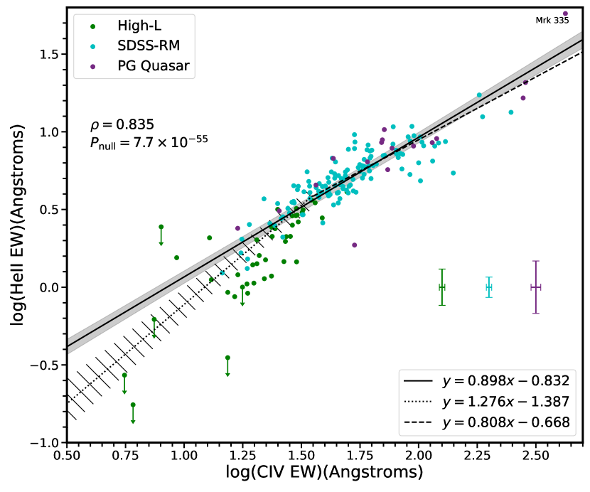
Figure 10: The  He ii EW as a function of  C iv EW for the quasars in our  He ii sample. The colors and symbols of the points are the same as in Figure 2. We find a strong correlation between these line EWs (Spearman statistics provided in the top left). We fit a power-law model (solid black line and grey region) to these data using the method from Kelly (2007) and present the functional form in the lower right-hand corner. The  C iv EW is a good indicator of the  He ii EW at large values (log( C iv EW) $>1.55$); however, the relationship seemingly diverges from the linear fit at low  C iv EW. We fit a power-law model to the data with log( C iv EW) $<1.55$ (black dotted line, hatched confidence interval) and to the data with log( C iv EW) $>1.55$ (dashed solid line, no confidence interval is shown since it overlaps well with the fit to the full data). The fit to the low  C iv EW data clearly diverges from the other two fits. This divergence might be the consequence of the quasar environment that affects  C iv, as discussed in Section 1.

We depict the  He ii EW as a function of  C iv EW in Figure 10. A Spearman test indicates that there is a strong correlation between the two parameters ($\rho=0.835$), and thus we fit a power-law relationship using the method from Kelly (2007). We find the best-fit relationship to be

$$\begin{split}\,\mbox{\text{C\,{iv}} EW}=(0.898\pm 0.0354)\rm{log}(\,\mbox{\text{He\,{ii}} EW})\\ -(0.832\pm 0.060);\sigma_{i}=0.075\pm 0.032,\end{split}$$ (3)

where $\sigma_{i}$ is the intrinsic dispersion in the relationship. Given that the observed scatter is $\sigma_{o}=0.138$, the uncertainty in the measurements, mainly in  He ii EW, accounts for a large fraction of the observed scatter. The tightness of the relationship is clearly demonstrated in Figure 10 at large values of  C iv EW where the power-law well represents the data. As the  C iv EW decreases, however, more scatter is apparent in the data around the model. In particular, at log₁₀( C iv EW) $<1.55$ Å, the data seemingly diverge from the power-law model. To quantify this non-linearity, we fit two additional power-law models to the data, one to the data points with log₁₀( C iv EW) $<1.55$ Å (dotted line in Figure 10, region represents the 1$\sigma$ confidence interval) and the other with log₁₀( C iv EW) $>1.55$ Å (dashed black line). The equations of these fits are provided in Figure 10, and the intrinsic scatter of the data around the fits to the low and high  C iv EW data are $\sigma_{i}=0.093\pm 0.056$ and $\sigma_{i}=0.074\pm 0.035$, respectively. The low  C iv EW power-law clearly exhibits a divergence from the rest of the data, and the fit suggests that the intrinsic scatter is mildly larger (albeit within $1\sigma$ of the other fits).

This apparent non-linear trend at low  C iv EW might be a consequence of the environmental effects discussed in Section 1 and 5.2 that affect  C iv EW but not  He ii EW. The small intrinsic scatter in this relationship further indicates that the measured  C iv EW is generally a good proxy for the strength of the ionizing continuum, particularly at large values of  C iv EW, and thus is a useful diagnostic of the quasar EUV ionizing SED in low signal-to-noise spectra where  He ii is difficult to measure. Aside from the mild non-linearity, this tight relationship indicates that the effects of the quasar environment upon  C iv EW are not typically strong, and theoretical models of quasar environments must be able to reproduce this behavior. Finally, given that most quasars do not have high-quality  X-ray coverage, the two power-law model enables us to predict the strength of the ionizing continuum from  C iv EW without having to compute $\alpha_{\rm{ox}}$. To assess how well this model can constrain the  He ii EW, we separated the data into small and large  C iv EW bins by splitting at log(C iv EW) $=1.55$. We then input the data from the small and large  C iv EW bins into the respective  He ii EW– C iv EW relationship presented at the bottom right-hand side of Figure 10 to predict  He ii EW. The residuals of the prediction to the measured  He ii EW were computed, and we found a $1\sigma$ spread in the residual to be $\approx$ 0.132. Since the residuals are calculated using logarithmic values, the difference can be expressed as the logarithm of the ratio of these values. Taking the inverse logarithm of the spread of the residuals indicates that the two power-law model can constrain the  He ii EW within a factor of $\approx 1.36$.

References

- Akritas & Siebert (1996) Akritas M. G., Siebert J., 1996, MNRAS, 278, 919
- Antonucci (2015) Antonucci R., 2015, arXiv e-prints, p. arXiv:1501.02001
- Baldwin (1977) Baldwin J. A., 1977, ApJ, 214, 679
- Baskin & Laor (2004) Baskin A., Laor A., 2004, MNRAS, 350, L31
- Baskin et al. (2013) Baskin A., Laor A., Hamann F., 2013, MNRAS, 432, 1525
- Baskin et al. (2014) Baskin A., Laor A., Stern J., 2014, MNRAS, 438, 604
- Baskin et al. (2015) Baskin A., Laor A., Hamann F., 2015, MNRAS, 449, 1593
- Bianchi et al. (2009) Bianchi S., Guainazzi M., Matt G., Fonseca Bonilla N., Ponti G., 2009, A&A, 495, 421
- Boroson & Green (1992) Boroson T. A., Green R. F., 1992, ApJS, 80, 109
- Brandt et al. (2000) Brandt W. N., Laor A., Wills B. J., 2000, ApJ, 528, 637
- Chiang & Murray (1996) Chiang J., Murray N., 1996, ApJ, 466, 704
- Davis & Tchekhovskoy (2020) Davis S. W., Tchekhovskoy A., 2020, ARA&A, 58, 407
- Dietrich et al. (2002) Dietrich M., Hamann F., Shields J. C., Constantin A., Vestergaard M., Chaffee F., Foltz C. B., Junkkarinen V. T., 2002, ApJ, 581, 912
- Elvis et al. (1994) Elvis M., et al., 1994, ApJS, 95, 1
- Fan et al. (2009) Fan L. L., Wang H. Y., Wang T., Wang J., Dong X., Zhang K., Cheng F., 2009, ApJ, 690, 1006
- Feigelson et al. (2014) Feigelson E. D., Nelson P. I., Isobe T., LaValley M., 2014, ASURV: Astronomical SURVival Statistics (ascl:1406.001)
- Ferland et al. (1992) Ferland G. J., Peterson B. M., Horne K., Welsh W. F., Nahar S. N., 1992, ApJ, 387, 95
- Filiz Ak et al. (2012) Filiz Ak N., et al., 2012, ApJ, 757, 114
- Foreman-Mackey et al. (2013) Foreman-Mackey D., Hogg D. W., Lang D., Goodman J., 2013, Publications of the Astronomical Society of the Pacific, 125, 306–312
- Fruscione et al. (2006) Fruscione A., et al., 2006, in Silva D. R., Doxsey R. E., eds, Society of Photo-Optical Instrumentation Engineers (SPIE) Conference Series Vol. 6270, Society of Photo-Optical Instrumentation Engineers (SPIE) Conference Series. p. 62701V, doi:10.1117/12.671760
- Gallagher et al. (2002) Gallagher S. C., Brandt W. N., Chartas G., Garmire G. P., 2002, ApJ, 567, 37
- Gallagher et al. (2006) Gallagher S. C., Brandt W. N., Chartas G., Priddey R., Garmire G. P., Sambruna R. M., 2006, ApJ, 644, 709
- Gibson et al. (2008) Gibson R. R., Brandt W. N., Schneider D. P., 2008, ApJ, 685, 773
- Giustini et al. (2008) Giustini M., Cappi M., Vignali C., 2008, A&A, 491, 425
- Goad & Korista (2014) Goad M. R., Korista K. T., 2014, MNRAS, 444, 43
- Green (1996) Green P. J., 1996, ApJ, 467, 61
- Green (1998) Green P. J., 1998, ApJ, 498, 170
- Green et al. (1986) Green R. F., Schmidt M., Liebert J., 1986, ApJS, 61, 305
- Guo et al. (2018) Guo H., Shen Y., Wang S., 2018, PyQSOFit: Python code to fit the spectrum of quasars, Astrophysics Source Code Library (ascl:1809.008)
- Inoue et al. (2007) Inoue H., Terashima Y., Ho L. C., 2007, ApJ, 662, 860
- Jones et al. (2001) Jones E., Oliphant T., Peterson P., et al., 2001, SciPy: Open source scientific tools for Python, http://www.scipy.org/
- Just et al. (2007) Just D. W., Brandt W. N., Shemmer O., Steffen A. T., Schneider D. P., Chartas G., Garmire G. P., 2007, ApJ, 665, 1004
- Kalberla et al. (2005) Kalberla P. M. W., Burton W. B., Hartmann D., Arnal E. M., Bajaja E., Morras R., Pöppel W. G. L., 2005, A&A, 440, 775
- Kaspi et al. (2005) Kaspi S., Maoz D., Netzer H., Peterson B. M., Vestergaard M., Jannuzi B. T., 2005, ApJ, 629, 61
- Kellermann et al. (1994) Kellermann K. I., Sramek R. A., Schmidt M., Green R. F., Shaffer D. B., 1994, AJ, 108, 1163
- Kelly (2007) Kelly B. C., 2007, ApJ, 665, 1489
- Kendall (1938) Kendall M. G., 1938, Biometrika, 30, 81
- Kendall (1970) Kendall M., 1970, Rank Correlation Methods. Theory and applications of rank order-statistics, Griffin, https://books.google.com/books?id=Mm2jjgEACAAJ
- Komossa et al. (2020) Komossa S., et al., 2020, A&A, 643, L7
- Korista et al. (1998) Korista K., Baldwin J., Ferland G., 1998, ApJ, 507, 24
- Kraft et al. (1991) Kraft R. P., Burrows D. N., Nousek J. A., 1991, ApJ, 374, 344
- Krawczyk et al. (2013) Krawczyk C. M., Richards G. T., Mehta S. S., Vogeley M. S., Gallagher S. C., Leighly K. M., Ross N. P., Schneider D. P., 2013, ApJS, 206, 4
- Kruczek et al. (2011) Kruczek N. E., et al., 2011, AJ, 142, 130
- Laor & Brandt (2002) Laor A., Brandt W. N., 2002, ApJ, 569, 641
- Laor & Davis (2014) Laor A., Davis S. W., 2014, MNRAS, 438, 3024
- Laor et al. (1995) Laor A., Bahcall J. N., Jannuzi B. T., Schneider D. P., Green R. F., 1995, ApJS, 99, 1
- Lawrence (2012) Lawrence A., 2012, MNRAS, 423, 451
- Lawrence (2018) Lawrence A., 2018, Nature Astronomy, 2, 102
- Leighly (2004) Leighly K. M., 2004, ApJ, 611, 125
- Liu et al. (2018) Liu H., Luo B., Brandt W. N., Gallagher S. C., Garmire G. P., 2018, ApJ, 859, 113
- Liu et al. (2020) Liu T., et al., 2020, ApJS, 250, 32
- Liu et al. (2021) Liu H., Luo B., Brandt W. N., Brotherton M. S., Gallagher S. C., Ni Q., Shemmer O., au2 J. D. T. I., 2021, On the Observational Difference Between the Accretion Disk-Corona Connections among Super- and Sub-Eddington Accreting Active Galactic Nuclei (arXiv:2102.02832)
- Luo et al. (2014) Luo B., et al., 2014, ApJ, 794, 70
- Luo et al. (2015) Luo B., et al., 2015, ApJ, 805, 122
- Lusso & Risaliti (2016) Lusso E., Risaliti G., 2016, ApJ, 819, 154
- Lusso & Risaliti (2017) Lusso E., Risaliti G., 2017, A&A, 602, A79
- Lusso et al. (2015) Lusso E., Worseck G., Hennawi J. F., Prochaska J. X., Vignali C., Stern J., O’Meara J. M., 2015, MNRAS, 449, 4204
- Lyons (1991) Lyons L., 1991, A Practical Guide to Data Analysis for Physical Science Students. Cambridge University Press
- MacLeod et al. (2010) MacLeod C. L., et al., 2010, ApJ, 721, 1014
- Miller et al. (2011) Miller B. P., Brandt W. N., Schneider D. P., Gibson R. R., Steffen A. T., Wu J., 2011, ApJ, 726, 20
- Netzer (2013) Netzer H., 2013, The Physics and Evolution of Active Galactic Nuclei
- Neugebauer et al. (1987) Neugebauer G., Green R. F., Matthews K., Schmidt M., Soifer B. T., Bennett J., 1987, ApJS, 63, 615
- Ni et al. (2018) Ni Q., et al., 2018, MNRAS, 480, 5184
- Pâris et al. (2018) Pâris I., et al., 2018, A&A, 613, A51
- Petrucci et al. (2018) Petrucci P. O., Ursini F., De Rosa A., Bianchi S., Cappi M., Matt G., Dadina M., Malzac J., 2018, A&A, 611, A59
- Piconcelli et al. (2005) Piconcelli E., Jimenez-Bailón E., Guainazzi M., Schartel N., Rodríguez-Pascual P. M., Santos-Lleó M., 2005, A&A, 432, 15
- Press et al. (1993) Press W. H., Teukolsky S. A., Vetterling W. T., Flannery B. P., 1993, Numerical Recipes in FORTRAN; The Art of Scientific Computing, 2nd edn. Cambridge University Press, 40 W. 20 St. New York, NY, USA
- Price-Whelan et al. (2018) Price-Whelan A. M., et al., 2018, AJ, 156, 123
- Pu et al. (2020) Pu X., Luo B., Brandt W. N., Timlin J. D., Liu H., Ni Q., Wu J., 2020, ApJ, 900, 141
- Rankine et al. (2020) Rankine A. L., Hewett P. C., Banerji M., Richards G. T., 2020, MNRAS, 492, 4553
- Reeves et al. (1997) Reeves J. N., Turner M. J. L., Ohashi T., Kii T., 1997, MNRAS, 292, 468
- Richards et al. (2006) Richards G. T., et al., 2006, AJ, 131, 2766
- Richards et al. (2011) Richards G. T., et al., 2011, AJ, 141, 167
- Rivera et al. (2020) Rivera A. B., Richards G. T., Hewett P. C., Rankine A. L., 2020, ApJ, 899, 96
- Schmidt & Green (1983) Schmidt M., Green R. F., 1983, ApJ, 269, 352
- Schneider et al. (2005) Schneider D. P., et al., 2005, AJ, 130, 367
- Schneider et al. (2010) Schneider D. P., et al., 2010, AJ, 139, 2360
- Scott et al. (2004) Scott J. E., Kriss G. A., Brotherton M., Green R. F., Hutchings J., Shull J. M., Zheng W., 2004, ApJ, 615, 135
- Shemmer & Lieber (2015) Shemmer O., Lieber S., 2015, ApJ, 805, 124
- Shemmer et al. (2008) Shemmer O., Brandt W. N., Netzer H., Maiolino R., Kaspi S., 2008, ApJ, 682, 81
- Shen et al. (2011) Shen Y., et al., 2011, ApJS, 194, 45
- Shen et al. (2015) Shen Y., et al., 2015, ApJS, 216, 4
- Shen et al. (2016) Shen Y., et al., 2016, ApJ, 831, 7
- Shen et al. (2019) Shen Y., et al., 2019, ApJS, 241, 34
- Smee et al. (2013) Smee S. A., et al., 2013, AJ, 146, 32
- Steffen et al. (2006) Steffen A. T., Strateva I., Brandt W. N., Alexander D. M., Koekemoer A. M., Lehmer B. D., Schneider D. P., Vignali C., 2006, AJ, 131, 2826
- Stevans et al. (2014) Stevans M. L., Shull J. M., Danforth C. W., Tilton E. M., 2014, ApJ, 794, 75
- Taylor (2005) Taylor M. B., 2005, in Shopbell P., Britton M., Ebert R., eds, Astronomical Society of the Pacific Conference Series Vol. 347, Astronomical Data Analysis Software and Systems XIV. p. 29
- Timlin et al. (2020a) Timlin J. D., Brandt W. N., Ni Q., Luo B., Pu X., Schneider D. P., Vivek M., Yi W., 2020a, MNRAS, 492, 719
- Timlin et al. (2020b) Timlin John D. I., Brandt W. N., Zhu S., Liu H., Luo B., Ni Q., 2020b, MNRAS, 498, 4033
- Timlin et al. (2021) Timlin J. D., Zhu S. F., Brandt W. N., Laor A., 2021, RNAAS, Submitted
- Vestergaard & Wilkes (2001) Vestergaard M., Wilkes B. J., 2001, ApJS, 134, 1
- Vietri et al. (2018) Vietri G., et al., 2018, A&A, 617, A81
- Waters et al. (2016) Waters T., Kashi A., Proga D., Eracleous M., Barth A. J., Greene J., 2016, ApJ, 827, 53
- Webb et al. (2020) Webb N. A., et al., 2020, A&A, 641, A136
- Wilkes & Elvis (1987) Wilkes B. J., Elvis M., 1987, ApJ, 323, 243
- Worrall et al. (1987) Worrall D. M., Giommi P., Tananbaum H., Zamorani G., 1987, ApJ, 313, 596
- Wu et al. (2011) Wu J., et al., 2011, ApJ, 736, 28
- York et al. (2000) York D. G., et al., 2000, AJ, 120, 1579
- Zheng & Malkan (1993) Zheng W., Malkan M. A., 1993, ApJ, 415, 517
- Zhu et al. (2020) Zhu S. F., Brandt W. N., Luo B., Wu J., Xue Y. Q., Yang G., 2020, MNRAS, 496, 245