Hubble Space Telescope UV and H$\alpha$ Measurements of the Accretion Excess Emission
from the Young Giant Planet PDS 70 b

Abstract

Recent discoveries of young exoplanets within their natal disks offer exciting opportunities to study ongoing planet formation. In particular, a planet’s mass accretion rate can be constrained by observing the accretion-induced excess emission. So far, planetary accretion is only probed by the H$\alpha$ line, . However, the majority of the accretion luminosity is expected to emerge from hydrogen continuum emission, In this paper, we present HST/WFC3/UVIS F336W (UV) and F656N (H$\alpha$) high-contrast imaging observations of PDS 70. Applying a suite of novel observational techniques, we detect the planet PDS 70 b with signal-to-noise ratios of 5.3 and 7.8 in the F336W and F656N bands, respectively. This is the first time that an exoplanet has been directly imaged in the UV. Our is higher by $3.5\sigma$ than the We estimate a mass accretion rate of $1.4\pm 0.2\times 10^{-8}M_{\mathrm{Jup}}\,\mathrm{yr}^{-1}$. H$\alpha$ accounts for 36% of the total accretion luminosity. Such a high proportion of energy released in line emission suggests efficient production of H$\alpha$ emission in planetary accretion, and motivates using the H$\alpha$ band for searches of accreting planets. These results demonstrate HST/WFC3/UVIS’s excellent high-contrast imaging performance and highlight its potential for planet formation studies.

1 Introduction

Directly imaged protoplanets are excellent testbeds for planet formation theories. These planets reside in the gaps of circumstellar disks, supporting models in which the observed protoplanetary disk gaps (e.g., Andrews et al., 2018) are carved by newly formed planets (e.g., Dodson-Robinson & Salyk, 2011; Zhu et al., 2011; Zhang et al., 2018; Bae et al., 2019). Ongoing accretion has been detected in these planets through their H$\alpha$ emission (Sallum et al., 2015; Wagner et al., 2018; Haffert et al., 2019; Hashimoto et al., 2020). The strength and velocity profile of the H$\alpha$ line can be used to indirectly constrain planetary mass accretion rates. These results enable quantitative investigations of accretion physics (e.g., Aoyama et al., 2018; Thanathibodee et al., 2019; Szulágyi & Ercolano, 2020), planet–disk interactions (e.g., Dong et al., 2015; Bae et al., 2019), and planetary luminosity evolution (e.g., Marley et al., 2007; Marleau et al., 2017).

PDS 70 is a ${\sim}{5}~{}\mathrm{Myr}$ old K7 T Tauri star in the Upper Sco association (Pecaut & Mamajek, 2016). The star is slowly accreting (Thanathibodee et al., 2020) and hosts a disk with complex structures including a giant inner cavity (Hashimoto et al., 2012; Keppler et al., 2019). Two planets, PDS 70 b and c, have been discovered within the disk cavity (Keppler et al., 2018; Haffert et al., 2019) located at projected separations of 20 and 34 AU from the star, respectively.

So far, mass accretion rate measurements for the PDS 70 planets have been solely based on observations of the H$\alpha$ line (e.g., Wagner et al., 2018; Haffert et al., 2019; Aoyama & Ikoma, 2019; Thanathibodee et al., 2019; Hashimoto et al., 2020; Aoyama et al., 2020). However, the intrinsic uncertainties in these relations are large and the validity of . The planetary accretion shock models (Aoyama & Ikoma, 2019; Thanathibodee et al., 2019; Szulágyi & Ercolano, 2020) all found that the H$\alpha$ emission and the accretion rate correlation for planets deviates from that for stars, due to differences in radiative transfer within the accretion shocks between protoplanets and protostars. Therefore, accurate planetary accretion rate measurements need both the H$\alpha$ line and hydrogen continuum emission. Because the likely contains the majority of the accretion luminosity, observing and measuring PDS 70 planets’ hydrogen continuum emission are particularly imperative.

Constraining the hydrogen continuum emission requires measuring the flux density on the blue side of the Balmer jump ($\lambda=3646\,\text{\AA}$) in the ultraviolet (UV). In this paper, we present Hubble Space Telescope/Wide Field Camera 3 (HST/WFC3) UVIS direct-imaging observations of the PDS 70 system in both the UV (F336W) and the H$\alpha$ line (F656N). We adopt a novel space-based angular differential imaging (ADI, Liu 2004; Marois et al. 2006) observational strategy to remove the contamination from the stellar point spread function (PSF) and measure the flux density of PDS 70 b. Using these measurements, we calculate the combined continuum$+$H$\alpha$ accretion luminosity, determine the H$\alpha{}$-to-continuum luminosity ratio, and derive the mass accretion rate for PDS 70 b. We then compare our measurement to previous accretion rate constraints of PDS 70 b, as well as to those of wide-orbit planetary-mass companions, brown dwarfs, and stars. Finally, we discuss the properties of PDS 70 b’s accretion-induced emission and its implication for the formation of this system.

2 Observations

We observed the PDS 70 system using HST/WFC3 in its UVIS channel for 18 HST orbits (Program GO-15830, PI: Zhou). All observations were conducted in the direct-imaging mode with the UVIS2/C512C subarray (field of view: $20.2^{\prime\prime}\times 20.2^{\prime\prime}$). The observations were constructed as six visit-sets, each consisting of three contiguous HST orbits. They were executed on UT dates starting on 2020-02-07, 2020-04-08, 2020-05-07, 2020-05-08, 2020-06-19, and 2020-07-03, respectively. As part of our angular differential imaging (ADI) strategy, the telescope orientation angle was increased by at least ten degrees from orbit to orbit. The telescope position angle (PA) ranged from $100.8^{\circ}$ to $297.0^{\circ}$, spanning $196.2^{\circ}$ in total.

We used the F336W ($\lambda_{\mathrm{eff}}=3359$ Å, FWHM $=550$ Å) and F656N ($\lambda_{\mathrm{eff}}=6561$ Å, $\mathrm{FWHM}=17.9$ Å) filters to measure the flux on the blue side of the Balmer jump and in the H$\alpha$ line, respectively. Each orbit consisted of ten 120 s F336W exposures and nine 20 s F656N exposures. Over 18 orbits, these observations amount to integration times of 21,600 s in F336W and 3240 s in F656N.

The WFC3/UVIS native spatial resolution (pixel scale$=40$ mas, FWHM ${\sim}1.75$ pixels) is below the Nyquist limit. To improve the spatial sampling of the images, we adopted a nine-point spiral dithering pattern. The dithering step was one half pixel (20 mas). For one cycle, the telescope pointing position started at a relative origin of (0, 0) and moved along a counterclockwise spiral track ((0, 0) $\rightarrow$ (0.5, 0) $\rightarrow$ (0.5,0.5) $\rightarrow\cdots\rightarrow$ (0.5, -0.5)). At every pointing, two exposures (one in each filter) were taken. Finally, the telescope returned to the origin and took one more F336W exposure. This dithering strategy enabled the reconstruction of images with spatial sampling of 20 mas, better than the Nyquist criterion.

3 Data Reduction

We start with the CalWFC3 pipeline-product flc files. These files are similar to the flat-field corrected flt files and have also been corrected for charge transfer efficiency losses. Our procedures include three main steps: (1) Nyquist-sampled image reconstruction; (2) primary star PSF subtraction using the Karhunen-Loève Image Processing (KLIP, Soummer et al. 2012) method; and (3) astrometry and photometry on the planet with PSF-subtracted images. We explain these three steps in the following subsections.

3.1 Up-sampling Images with the Fourier Reconstruction Method

We combine dithered images using the Fourier reconstruction method (Lauer, 1999). Compared to the astrodrizzle method (which produces the drz files available in the STScI archive), the Fourier reconstruction method guarantees Nyquist sampling and is optimized point-source PSFs. It has previously been applied in high-contrast imaging observations of exoplanets (Rajan et al., 2015).

We implement the Fourier reconstruction method as a python-based pipeline. We first test the pipeline using model PSFs produced by the TinyTim software (Krist et al., 2011) and confirm that the difference between the reconstructed and the true PSFs is less than 1% in intensity per pixel. Then, we apply the pipeline to our observations. We reconstruct two images per orbit per filter. Each image is a combination of five dithered exposures. For the F336W band, the two reconstructed images are combined from exposures 1-5 and 6-10. For the F656N band, because one orbit of observations consists of nine exposures, the first exposure (for which the pointing is at the origin) is shared by both reconstructions. The size of dithering steps as executed is determined using the World Coordinate System target pointing information provided in the fits file header. Finally, we apply a geometric distortion correction to the reconstructed images using the solution in Bellini et al. (2011). In total, we obtain 36 up-sampled (19.8 mas/pixel image scale, FWHM=3.5 pixels) and geometrically rectified images for each band.

3.2 Primary Star PSF Subtraction

We use the KLIP algorithm (Soummer et al., 2012) to subtract the PSF of the primary star. The algorithm is performed on a $128{\times}128$ pixel ($2\farcs 51\times 2\farcs 51$) subarray centered on PDS 70. First, we coalign the images by carrying out two-dimensional (2D) Gaussian fits on the PSF core of PDS 70 and shifting the images with bi-cubic interpolation. We then select reference PSF images for each target image. To avoid self-subtraction of the astronomical signals, we impose a minimum limit of $35^{\circ}$ difference in the telescope roll angle between the reference image and the target image. This criterion ensures that at the separation of PDS 70 b (170 mas) the PSFs are separated by at least 1.5 FWHMs between the target and reference images. To avoid cross-subtraction between PDS 70 b and c, we exclude reference images in which the PSFs of PDS 70 c are within 1 FWHM distance of PDS 70 b in the target image and vice versa. After selection, each target image has between 15 and 22 reference images.

KLIP is performed in parallel on subregions of the images. We experiment with various geometries for subdividing the images and select the one that results in the best planet detection SNRs. In the optimal solution, the target image is divided into annular sectors with radial bounds at 100, 350, and 700 mas. This division also defines our inner working angle to be 100 mas. Each annulus is further divided into three equal-size sectors, each spanning $120^{\circ}$. We run separate KLIP reductions to optimize for PDS 70 b and c individually. The planet being optimized for is placed in the center of an annular sector. After primary subtraction, we derotate the images to align their $y$-axis to the north. Finally, we register all derotated and primary-subtracted images by the centroid of PDS 70, align them using cubic interpolation shift, and combine the aligned images using the inverse-variance weighting method (Bottom et al., 2017). Figure 1 shows the primary-subtracted images. Point sources that match the expected position of PDS 70 b are detected in both bands. PDS 70 c is not detected in either band.

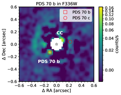
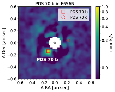
Figure 1: Primary-subtracted images in up-sampled resolution (20 mas per pixel) of the PDS70 system in the F336W (left) and F656N (right) bands. PDS70b is detected in both bands. Another close candidate companion (CC) is identified in the F336W image at $\mathrm{PA}{\sim}310$ and $\mathrm{sep}{\sim}110$ mas. To reduce high frequency noise, we smooth these images with a Gaussian kernel with a FWHM of 2.8 pixels (80% of the PSF FWHM). The expected positions of PDS 70 b and c, which are from their most recent astrometry (Wang et al., 2020), are shown in red squares and circles, respectively. North is up and east is to the left.

3.3 Photometry and Astrometry of PDS 70 b

We conduct photometric and astrometric measurements of PDS 70 b using the KLIP forward modeling method (Pueyo, 2016). This technique calibrates measurement biases introduced in primary subtraction procedures. In our implementation, we inject the forward modeling signals into the original frame before the image reconstruction step, so it also addresses possible systematics caused by image reconstruction. We use TinyTim PSFs (Krist et al., 2011) to model the astrophysical signals. Negative-flux PSFs are injected at and around the expected position of PDS 70 b in the original undersampled images. When the injected PSF matches the true signal in intensity and position, it cancels out the astrophysical signal and, therefore, locally minimizes the residuals in the primary-subtracted images. The injected PSF is sampled on a $10\times 10\times 10$ grid of flux density, PA, and separation. At each grid point, we run a complete data reduction and calculate the residual sum of squares (RSS) within an annular sector ($\theta=80^{\circ},r_{\mathrm{in}}=100\,\mathrm{mas},r_{\mathrm{out}}=240\,\mathrm{mas}$, centered on PDS 70 b). We find that the RSS follows a parabolic function of the injected flux, PA, and separation, which is the expected outcome when the measurement biases are caused by “over-subtraction” instead of “self-subtraction” (Apai et al., 2016; Pueyo, 2016). We use the minimum of each best-fit parabola as the final measurements for the flux density, PA, and separation of PDS 70 b.

3.4 Injection-and-Recovery Tests

We estimate the KLIP throughput and its uncertainty by injecting and recovering TinyTim model PSFs (Krist et al., 2011) that have the same flux densities as PDS 70 b. In each round of the injection-and-recovery test, we first inject five PSFs at the same PA but different separations of 173, 300, 450, 600, and 800 mas so that the innermost one has the same separation as PDS 70 b. We also subtract an identical PSF at the position of PDS 70 b to mitigate its interference with the test. We then perform KLIP with the same setups as those in §3.2 and conduct photometry on the primary-subtracted image (Figure 2) for each injected PSF to obtain its recovered flux. The throughput factor is determined as the ratio between the recovered and the injected flux. We repeat this test for thirteen evenly spaced PAs that differ from the PA of PDS 70 b for at least $60^{\circ}$. We take the averages of the thirteen iterations as the azimuthal-averaged throughputs and the standard deviations as the throughput uncertainties. Figure 2 shows examples of primary-subtracted images that contain injected PSFs.

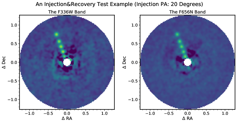
Figure 2: Examples of injection-recovery tests in the F336W (left) and F656N (right) bands. TinyTim PSFs with the same flux densities as PDS70b are injected at a PA of 20 degrees and separations at 173, 300, 450, 600, and 800 mas. The innermost injected PSF has the same separation as PDS70b. Five injected planets are recovered in both bands. PDS 70 b is removed from the images by subtracting its best-fit PSF model to mitigate its interference with the test. The same tests are repeated at another twelve position angles.

3.5 Signal-to-noise Ratio and Uncertainty Analyses

We calculate the planet detection SNRs following the procedures described in Mawet et al. (2014). This method properly accounts for small number statistics at close separations in high-contrast imaging data. First, we integrate the planetary signals in the primary-subtracted images using a 1.0 FWHM (3.5 pixels) diameter aperture. We position the aperture centered on the location of PDS 70 b as determined by a 2D Gaussian fit. We then estimate the background level and noise. Aperture-integrated fluxes are taken in non-overlapping 1.0 FWHM diameter apertures located and distributed azimuthally at the same separation as the detected point source (Figure 3). We insert the mean and standard deviations of these flux values into Equation (9) of Mawet et al. (2014) to derive the detection SNRs.

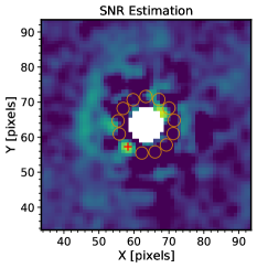
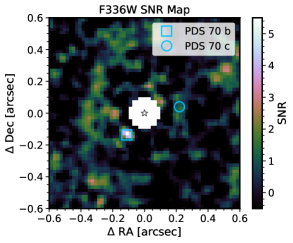
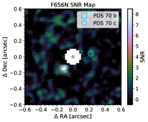
Figure 3:

The photometric uncertainty consists of three components: the speckle noise, the photon noise, and the KLIP throughput uncertainty. Speckle noise is determined from the standard deviation of the flux integrated within the apertures illustrated in Figure 3. This component also accounts for possible contamination from the circumstellar disk. Photon noise is the square root of the total number of photons collected over the 18 orbits of observations. The KLIP throughput uncertainty is derived in §3.4. For both bands, speckle noise is the dominant component of the total error budget. It is more than ten times greater than the photon noise and a few times greater than the KLIP throughput uncertainty. We assume that these three components are independent and combine them in quadrature. For astrometric error estimation, we assume the radial and tangential directions are independent and calculate their uncertainties as FWHM/SNR.

4 Results

4.1 Flux densities and the position of PDS 70 b

We detect PDS 70 b in the F336W and F656N bands with aperture-integrated SNRs of 5.3 and 7.9, respectively. These SNRs correspond to false positive probabilities of $9.4\times 10^{-5}$ and $8.1\times 10^{-7}$ based on Student’s $t$-test statistics (Mawet et al., 2014). The average planet-to-star brightness contrast ratios are $3.25\pm 0.66\times 10^{-4}$ and $1.38\pm 0.19\times 10^{-3}$ in the two bands. Neither band yields an $\mathrm{SNR}>2$ detection for PDS 70 c (see §4.4).

Our photometry for PDS 70 b yields count rates $1.12\pm 0.22$ $\mathrm{e^{-}\,s^{-1}}$ and $5.70\pm 0.79$ $\mathrm{e^{-}\,s^{-1}}$ in the F336W and the F656N bands, respectively. We convert count rates to flux densities ($f_{\lambda}$ in $\mathrm{erg\,s^{-1}\,cm^{-2}\,\text{\AA}^{-1}}$) using the PHOTFLAM inverse sensitivity factors provided in the fits file headers. This results in $f_{\lambda,\,\mathrm{F336W}}=1.4\pm 0.3\times 10^{-18}\mathrm{erg\,s^{-1}cm^{-2}\text{\AA}^{-1}}$ and $f_{\lambda,\,\mathrm{F656N}}=9.2\pm 1.3\times 10^{-17}\mathrm{erg\,s^{-1}cm^{-2}\text{\AA}^{-1}}$. We derive PDS 70 b’s H$\alpha$ line flux by multiplying $f_{\lambda,\,\mathrm{F656N}}$ by the effective bandpass of the F656N filter ($17.65\,\text{\AA}$), and find it to be $\mathcal{F_{\mathrm{F656N}}}=1.62\pm 0.22\times 10^{-15}\mathrm{erg\,s^{-1}cm^{-2}}$.

We determine PDS 70 b’s position angles and separations in the two bands separately. The results are $\mathrm{PA}=139.9\pm 5.0^{\circ}$, $\mathrm{sep}=163\pm 14$ mas in F336W and $\mathrm{PA}=143.4\pm 3.0^{\circ}$, $\mathrm{sep}=177.0\pm 9.4$ mas in F656N. The uncertainties in the F336W band are greater due to the lower detection SNR. As demonstrated in Figure 4, PDS 70 b’s positions in the two bands are consistent within $1\sigma$ .

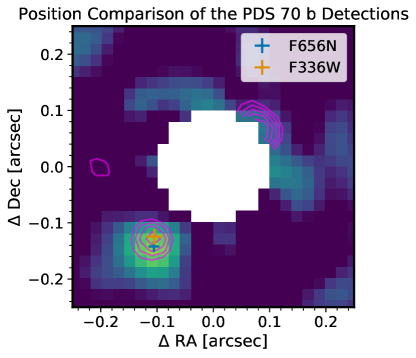
Figure 4: A comparison of the positions of the point sources detected in the F336W and F656N bands. Contours (30%, 40%, 50%, 60%, and 70% of the maximum pixel value) of the F336W image are overlaid on the F656N image. The F336W contours match the position of the PDS 70 b’s detection in F656N. The two crosses mark the best-fit positions of PDS70 b in the two bands. The sizes of the crosses represent the $1\sigma$ uncertainties. The proximity of the two crosses indicates that PDS 70 b’s detections in the two bands are consistent with each other in their positions.

We also identify excess emission of a close candidate companion (CC) at $\mathrm{PA}{\sim}310^{\circ}$ and $\mathrm{sep}{\sim}110$ mas in the F336W image. The location is close to the inner working angle (100 mas). The detection SNR is ${\sim}2.5$, corresponding to a false positive probability of 1.8%. Mesa et al. (2019) reported a point-like feature at a similar location in their VLT/SPHERE observations. Based on its near-infrared spectrum, Mesa et al. (2019) interpreted it as scattered starlight from circumstellar material.

4.2 Contrast Curves

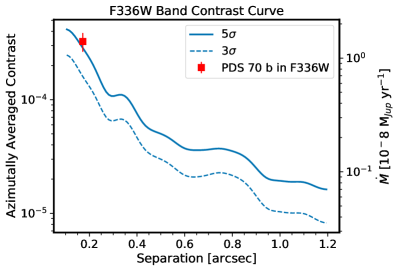
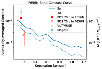
Figure 5: Azimuthally averaged contrast curves in the F336W and F656N bands. Blue solid and dashed lines represent the $5\sigma$ and $3\sigma$ contrast curves, respectively. The secondary $y$-axes show the corresponding sensitivity in $\dot{M}$ of a PDS 70 b-like planet. We convert contrast ratios to $\dot{M}$ sensitivities based on Equation 2. The red squares are the observed contrasts for PDS 70 b. In the right panel, the open red square marks the aperture-integrated signal at the expected position of PDS 70 c. The right panel also shows ground-based H$\alpha$ contrast measurements of PDS 70 b and c (Wagner et al., 2018; Hashimoto et al., 2020).

The contrast curves, defined as the flux ratio of the detection limit and PDS 70, are presented in Figure 5. We use the method of §3.5 to estimate the $3.5\,\mathrm{pixels}$ diameter aperture-integrated detection limit and then apply aperture and throughput corrections to account for the finite aperture size and over-subtraction. Aperture correction coefficients are determined by interpolating the WFC3/UVIS2 encircled energy table. Throughput calibration factors are derived with the injection-and-recovery tests (see §3.4). For separations that are not in the injection-and-recovery tests, the linearly interpolated (or extrapolated) values are used. The PDS 70’s flux densities are the time-averaged values over the entire observations. Based on the contrast curves, the F336W image is more sensitive than the F656N by a factor of 3–4, depending on the separation. The 5$\sigma$ detection limit in F336W reaches a contrast of $1.1\times 10^{-4}$ at 0.3 arcsec and $2.0\times 10^{-5}$ at 1 arcsec. In the F656N band, these limits are $4.6\times 10^{-4}$ and $6.8\times 10^{-5}$, respectively.

For comparison, we overplot the observed contrasts of PDS 70 b in F336W and F656N, as well as the H$\alpha$ contrasts of PDS 70 b and c measured in MagAO (Wagner et al., 2018) and VLT/MUSE (Haffert et al., 2019; Hashimoto et al., 2020) observations. To account for the filter bandpass and spectral resolution differences, we calibrate these H$\alpha$ contrasts and unify them under the WFC3/UVIS2/F656N system. We adopt the planets’ absolute H$\alpha$ flux (Wagner et al., 2018; Hashimoto et al., 2020) and divide them by the F656N band-integrated flux of PDS 70 ($\mathcal{F}_{\mathrm{PDS\,70,\,F656N}}=1.18\times 10^{{-12}}\,\mathrm{erg\,cm^{-2}s^{-1}}$). These observations demonstrate clear disagreement in PDS 70 b’s H$\alpha$ contrasts. As for PDS 70 c, its H$\alpha$ contrast estimated by VLT/MUSE is below our $3\sigma$ sensitivity limit.

4.3 Time-resolved Photometry of PDS 70 b in H$\alpha$

All F656N images from the six individual visit-sets yield SNR$>3$ detections of PDS 70 b. Following the procedures of §3.3 and 3.5, The average flux is within $1\sigma$ uncertainty of every time-resolved measurement except Visit-set 3, which has the strongest H$\alpha$ flux. However, the H$\alpha$ flux in Visit-set 3 is only $1.4\sigma$ greater than the average of the rest of the observations. Based on the uncertainty of the light curve, we place an upper limit of $30\%$ variability for PDS 70 b in H$\alpha$

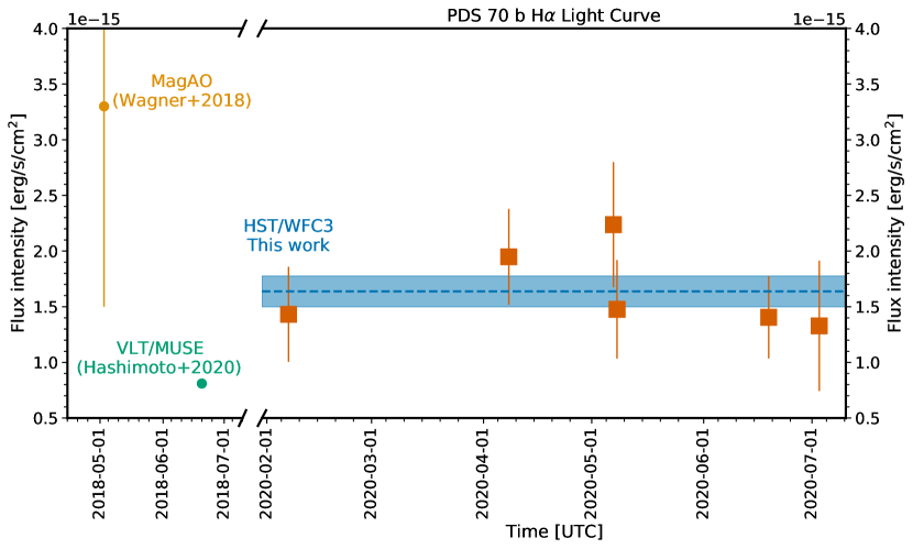
Figure 6: Time-resolved H$\alpha$ flux of PDS70b. Red squares and errorbars are PDS70 b’s H$\alpha$ flux in individual visit-sets. The blue dashed line and rectangle shade show the average HST flux and its $1\sigma$ uncertainty, respectively.

We also compare PDS 70 b’s H$\alpha$ flux in our HST observations to ground-based measurements from MagAO (Wagner et al., 2018), and VLT/MUSE (Haffert et al., 2019; Hashimoto et al., 2020). The HST measurement of $1.62\pm 0.23\times 10^{-15}\,\mathrm{erg\,s^{-1}\,cm^{-2}}$ is lower than the MagAO result of $3.3\pm 1.8\times 10^{-15}\,\mathrm{erg\,s^{-1}\,cm^{-2}}$ (Wagner et al., 2018) but the difference is within $1\sigma$. Our result is higher than the VLT/MUSE flux of $0.81\pm 0.03\times 10^{-15}\,\mathrm{erg\,s^{-1}\,cm^{-2}}$, (Hashimoto et al., 2020) by $3.5\sigma$, which may suggest significant H$\alpha$ variability on ${\sim}1$-2 years timescales. Follow-up observations with the same instrument and consistent flux calibrations are necessary to

4.4 The Nondetection of PDS 70 c

Neither the F336W nor the F656N image yields an $\mathrm{SNR}>2$ detection for PDS 70 c. The nondetection of PDS 70 c in the F656N band is consistent with its H$\alpha$ flux measurements reported by Haffert et al. (2019) and Hashimoto et al. (2020). Using the method of §3.5, we calculate the aperture-integrated (diameter=3.5 pixels) SNR at PDS 70 c’s expected position ($\mathrm{PA}{=}280^{\circ}$, $\mathrm{sep}{=}223$ mas, Wang et al. 2020) in the F656N image and obtain a result of $\mathrm{SNR}{=}1.4$ (false positive probability of 9.5%). The corresponding aperture and throughput-corrected H$\alpha$ flux is $2.6\pm 1.9\times 10^{-16}\mathrm{erg\,s^{-1}cm^{{-2}}}$, consistent with the VLT/MUSE measurement of $3.1\pm 0.3\times 10^{-16}\mathrm{erg\,s^{-1}cm^{{-2}}}$ within $1\sigma$. However, such a low flux does not permit a statistically significant detection in our observations. As shown in Figure 5, both our observed H$\alpha$ flux at the position of PDS 70 c and the literature value are below the 3$\sigma$ detection limit. As for the F336W band, we expect the planet is even less likely to be detected due to greater star-to-planet brightness contrast. Therefore, these nondetections are most likely due to our sensitivity limits.

5 Accretion onto PDS 70 b

5.1 Estimating the Accretion Luminosity and Mass Accretion Rate of PDS 70 b

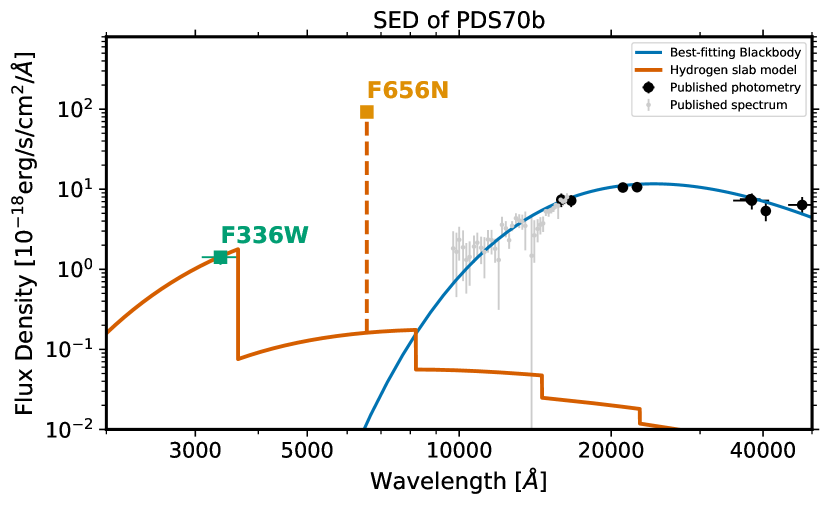
Figure 7: The UV, optical, and IR SED of PDS 70 b. The green and orange squares show the observed flux densities of PDS 70 b in the F336W and F656N bands, respectively. These flux densities are more than three orders of magnitude higher than the $1.2\times 10^{3}$ K blackbody (blue curve) that is the best-fit model to the planet’s IR observations (gray and black dots; data taken from Müller et al. 2018; Mesa et al. 2019; Wang et al. 2020; Stolker et al. 2020). The vertical dashed line indicates the position of H$\alpha$ and the red solid curve represents a hydrogen continuum emission model spectrum. We use this model to conduct bolometric correction for the F336W photometry.

The F336W and F656N bands constrain hydrogen Balmer continuum and H$\alpha$ emission, both of which are accretion indicators (Aoyama et al., 2020). As shown in the UV, optical, and IR spectral energy distribution (SED) of PDS 70 b (Figure 7), our observed F336W and F656N flux densities are more than three orders of magnitude higher than the best-fit blackbody to the infrared (IR) observations. This suggests that accretion-induced hydrogen emission dominates the flux in the F336W and F656N bands and the contribution from the blackbody continuum can be safely ignored. Therefore, we can measure the accretion luminosity ($L_{\mathrm{acc}}$) with the F336W and F656N flux densities and then convert the accretion luminosity to a mass accretion rate ($\dot{M}$).

To calculate $L_{\mathrm{acc}}$, we need to introduce four assumptions:

1. H$\alpha$ dominates the hydrogen line emission.

2. We adopt a plane parallel pure hydrogen slab model (Valenti et al., 1993) to conduct a bolometric correction for the F336W flux density and derive $L_{\mathrm{cont}}$. This model calculates the hydrogen bound-free emission spectrum as a function of temperature, number density ($n$), slab length, and the filling factor. Herczeg & Hillenbrand (2008), Herczeg et al. (2009), and Zhou et al. (2014) used the same model for their bolometric corrections.

3. The hydrogen number density of the slab is $10^{13}\mathrm{cm^{-3}}$. This number density is consistent with the estimates in Aoyama & Ikoma (2019) and Hashimoto et al. (2020) and leads to a relatively large Balmer jump (a flux ratio of 17) compared to those typically observed in classical T Tauri stars (flux ratio $<3$; e.g., Valenti et al., 1993; Calvet & Gullbring, 1998; Alcalá et al., 2014), .

4. We assume no extinction for PDS 70 b and do not de-redden the observed flux densities.

We first use these assumptions to derive PDS 70 b’s $L_{\mathrm{acc}}$ and then discuss their impact on the results.

$L_{\mathrm{acc}}$ is the sum of two parts: the hydrogen line emission luminosity ($L_{\mathrm{line}}$) and the hydrogen continuum emission luminosity ($L_{\mathrm{cont}}$):

$$L_{\mathrm{acc}}=L_{\mathrm{line}}+L_{\mathrm{cont}}.$$ (1)

To estimate the line emission flux, we apply Assumption (1) to get $L_{\mathrm{line}}$ =$L_{\mathrm{H\alpha}}$. To calculate the continuum emission flux, we conduct a bolometric correction to the F336W flux density using the hydrogen continuum spectrum model determined by Assumption (2) and (3). The continuum model spectrum is scaled so that it produces the observed F336W flux density. Integrating the scaled model over its entire spectral range results in the continuum flux. We convert flux to luminosity by multiplying by $4\pi d^{2}$, where $d$ is PDS 70’s Gaia DR2 distance (113.06 pc, Gaia Collaboration et al., 2016, 2018; Bailer-Jones et al., 2018). This gives $L_{\mathrm{line}}=6.5\pm 0.9\times 10^{-7}L_{\odot}$, $L_{\mathrm{cont}}=1.2\pm 0.2\times 10^{-6}L_{\odot}$, and $L_{\mathrm{acc}}=1.8\pm 0.2\times 10^{-6}L_{\odot}$.

We assume a magnetospheric accretion model to convert accretion luminosity to mass accretion rate ($\dot{M}$). Following Gullbring et al. (1998), we have

$$\dot{M}=\Bigl{(}1-\frac{R_{\mathrm{p}}}{R_{\mathrm{in}}}\Bigr{)}\frac{R_{\mathrm{p}}}{GM_{\mathrm{p}}}L_{\mathrm{acc}}.$$ (2)

The accretion flow is launched at the magneto-truncation radius of $R_{\mathrm{in}}$ and free-falls onto the planetary surface. The entire kinetic energy of the accretion flow is converted to accretion luminosity. We follow Gullbring et al. (1998) and assume $R_{\mathrm{in}}=5R_{\mathrm{p}}$ Inserting our measured value of $L_{\mathrm{acc}}$ ($1.8\pm 0.2\times 10^{-6}L_{\odot}$) and the latest mass ($1M_{\mathrm{Jup}}$) and radius ($1.75R_{\mathrm{Jup}}$) estimates (Stolker et al., 2020), we get

$$\dot{M}=1.4\pm 0.2\times 10^{-8}\Bigl{(}\frac{R_{\mathrm{p}}}{1.75R_{\mathrm{Jup}}}\Bigr{)}\Bigl{(}\frac{M_{\mathrm{p}}}{1M_{\mathrm{Jup}}}\Bigr{)}^{-1}M_{\mathrm{Jup}}\,\mathrm{yr^{-1}}.$$ (3)

The quoted uncertainty in $\dot{M}$ contains those propagated from $L_{\mathrm{acc}}$ but not systematic uncertainties of $\dot{M}$.

Equation 2 provides a correspondence between the contrast ratio (Figure 5) and $\dot{M}$ of a PDS 70 b-like planet. Because accretion excess emission dominates the planet’s flux in the F336W and F656N bands and $\dot{M}$ scales linearly with $L_{\mathrm{acc}}$ (when constant mass and radius are assumed), the contrast ratio should also scale linearly with $\dot{M}$. We conduct the contrast ratio to $\dot{M}$ conversion and show the results as the secondary $y$-axes of Figure 5. At $1\arcsec$ separation, both bands are sensitive to $\dot{M}$ of $10^{-9}M_{\mathrm{Jup}}\,\mathrm{yr^{-1}}$ accretion onto a PDS 70 b-like planet.

5.2 Systematic Uncertainties in the Accretion Rate Estimate

Systematic uncertainties in our accretion rate estimate for PDS 70 b are similar to those of other (sub)stellar accretion measurements made with $U$-band spectrophotometry (e.g., Herczeg & Hillenbrand, 2008). There are four sources of systematics: bolometric correction for the continuum luminosity, neglected emission lines, uncertain accretion mechanisms, and the unknown extinction.

The bolometric correction is directly set by the size of the Balmer jump, which is unconstrained by our observations. For our analysis, we fix the number density of the hydrogen slab to $1\times 10^{{13}}$cm^-3, resulting in a factor of 17 flux increase at the Balmer jump. This number density is low compared to those adopted in stellar accretion rate analyses (e.g., Valenti et al., 1993; Gullbring et al., 1998; Ingleby et al., 2013), but consistent with the results from analyzing PDS 70 b’s H$\alpha$ line profile (Hashimoto et al., 2020). Increasing the number density by one order of magnitude will decrease the Balmer jump size to 4, increase the bolometric correction factor by 20%, and increase the accretion rate measurement by 12%.

We include only H$\alpha$ for calculating $L_{\mathrm{line}}$. Because line emission accounts for a greater amount of accretion luminosity in the substellar regime (Herczeg et al., 2009; Rigliaco et al., 2012; Zhou et al., 2014), excluding other lines may introduce greater errors in $\dot{M}$ for PDS 70 b compared to similar measurements in the stellar regime (e.g., Herczeg & Hillenbrand, 2008). Based on a planetary accretion shock model, Aoyama et al. (2018, 2020) found that the Ly$\alpha$ emission can be more than one order of magnitude more energetic than the H$\alpha$ emission in accretion onto PDS 70 b-like planets. In this case, the hydrogen line emission will dominate PDS 70 b’s accretion excess emission. In the case where PDS 70 b’s $L_{\mathrm{line}}$ is the same as its $L_{\mathrm{cont}}$, the accretion rate will be increased by 26% compared to the Equation 3 result.

By adopting Equation 2, we assume the accretion flow is launched 5$R_{\mathrm{p}}$ away from the planet and hits the planetary surface. When a different accretion paradigm is assumed (e.g., Szulágyi & Ercolano, 2020), as long as the kinetic energy of the accretion flow is entirely converted to accretion luminosity, Equation 2 should still hold. Based on Equation 2, the accretion rate is correlated with the assumed radius and anticorrelated with the assumed mass. An overestimated radius or an underestimated mass will lead to an overestimated accretion rate, and vice versa.

The lack of a tight constraint on the line-of-sight extinction of PDS 70 b leads to the most significant systematic uncertainty in our $\dot{M}$ estimate. Because extinction is much more effective in the F336W band than at H$\alpha$ ($A_{\mathrm{F336W}}/A_{\mathrm{H\alpha}}=2.0$, assuming $R_{V}=3.1$, Cardelli et al. 1989), accretion luminosity estimate increases with extinction at a much steeper rate in our analysis than those solely based on H$\alpha$ (Wagner et al., 2018; Aoyama & Ikoma, 2019; Hashimoto et al., 2020, Figure 8). In the high extinction scenario ($A_{V}>3$ mag) adopted in Hashimoto et al. (2020), the mass accretion rate of PDS70 b will be $\dot{M}{\sim}7\times 10^{-7}M_{\mathrm{Jup}}\,\mathrm{yr}^{-1}$, two orders of magnitude greater than the result assuming zero extinction.

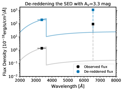
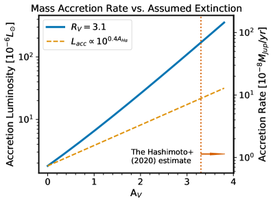
Figure 8: Extinction affecting the accretion luminosity and accretion rate measurements for PDS 70 b. Left: comparison between the observed flux densities and the dereddened one for which high extinction of $A_{V}=3.3$ mag is assumed. Dereddening increases the flux in both bands, but much more significantly in the F336W band. Right: accretion luminosity and accretion rate results as a function of the assumed extinction magnitude. The orange dashed line shows that the trend for accretion luminosity scales as $10^{0.4A_{H\alpha}}$, which was assumed in Wagner et al. (2018), Aoyama & Ikoma (2019), and Hashimoto et al. (2020). Because reddening is stronger at shorter wavelengths, accretion luminosity estimates increase with $A_{V}$ at a much greater rate in our analysis (blue solid line) that calculates accretion excess emission in both UV and H$\alpha$. In the high extinction scenario (Hashimoto et al., 2020), extinction increases the $L_{\mathrm{H\alpha}}+L_{\mathrm{cont}}$ estimate for $L_{\mathrm{acc}}$ (blue line) by nearly one order of magnitude stronger compared to the scenario in which only $A_{H\alpha}$ is considered.

5.3 Accretion-induced Emission: Line versus Continuum

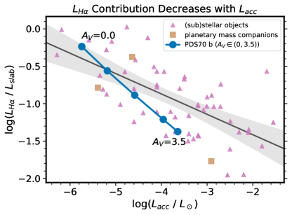
Figure 9: The relation between $L_{\mathrm{H\alpha}}$ and $L_{\mathrm{acc}}$ for PDS70b (this work), planetary-mass companions (Zhou et al., 2014), brown dwarfs, and low-mass ($<0.2\,M_{\odot}$) stars (Herczeg & Hillenbrand, 2008; Herczeg et al., 2009; Rigliaco et al., 2012; Alcalá et al., 2014, 2017). The blue line tracks $L_{\mathrm{H\alpha}}$/$L_{\mathrm{acc}}$ for PDS70b for $A_{V}$ from 0 to 3.5. The gray line is the linear regression of $\log(L_{\mathrm{H\alpha}}/L_{\mathrm{acc}})$ and $\log(L_{\mathrm{acc}})$, indicating a trend that low accretion luminosity objects release a greater proportion of their accretion energy in the H$\alpha$ line. Our measurements for PDS70b agree well with the general trend. In particular, the $A_{V}=0$ value falls within the expected range based on this linear regression.

PDS 70 b’s H$\alpha$-to-continuum accretion luminosity ratio is $L_{\mathrm{H\alpha}}/L_{\mathrm{cont}}=0.56$. Such a high H$\alpha$ contribution to the total accretion excess emission is similar to those observed in the accreting planetary-mass companions GSC06214-0210b and DH Tau b (Zhou et al., 2014), as well as a few other slowly accreting substellar objects (Figure 9, Herczeg & Hillenbrand, 2008; Herczeg et al., 2009; Rigliaco et al., 2012; Alcalá et al., 2014, 2017). This ratio decreases if a greater extinction magnitude is assumed. Dereddening the photometry with an extinction law of $A_{V}=2\,\mathrm{mag}$ ($R_{V}=3.1$) reduces $L_{\mathrm{H\alpha}}/L_{\mathrm{cont}}$ to ${\sim}10\%$.

PDS 70 b’s high H$\alpha$ emission contribution to the total accretion luminosity is likely rooted in its planetary mass and relatively weak accretion flow (Aoyama et al., 2018). Compared to stars, PDS 70 b’s accretion shock likely has a lower hydrogen number density (Aoyama & Ikoma, 2019; Hashimoto et al., 2020), resulting in optically thin emission with stronger line emission and high Balmer jump (e.g., Herczeg et al., 2009). In addition, Aoyama & Ikoma (2019) found that in planetary accretion shocks, H$\alpha$ is emitted from the post-shock gas. This is in contrast to the stellar magnetospheric accretion scenario where H$\alpha$ comes from the pre-shock flows (e.g., Muzerolle et al., 1998; Alencar et al., 2012). This difference further increases the line-to-continuum luminosity ratio in planetary accretion emission. Our observations directly confirm the divergence between the accretion of PDS 70 b and accretion in young stellar objects.

Our results also reinforce the danger of extrapolating empirical stellar $L_{\mathrm{H\alpha}}-L_{\mathrm{acc}}$ relations (Rigliaco et al., 2012; Ingleby et al., 2013; Alcalá et al., 2014) into the planetary accretion regimes, which has been previously identified in theoretical studies (e.g., Aoyama et al., 2018; Thanathibodee et al., 2019; Szulágyi & Ercolano, 2020). Those linear relations cannot fully capture the diversity in the mechanisms of accretion excess emission between the planetary and stellar scenarios. Our measurements of both $L_{\mathrm{H\alpha}}$ and $L_{\mathrm{cont}}$ offer a more direct way to probe the mass accretion rate of PDS70b. The high $L_{\mathrm{H\alpha}}/L_{\mathrm{cont}}$ ratio of PDS 70 b significantly improves its star-to-planet contrast in the H$\alpha$ band, which may serve as further motivation to search for accreting giant planets with H$\alpha$ (e.g., Zurlo et al., 2020; Close, 2020)

5.4 A Comparison to Measurements Based on Accretion Models

5.5 The Mass Accretion Rate of PDS 70 b in Context

The mass accretion rate of young stellar objects follows a power law in stellar mass, albeit with considerable uncertainty. With our mass accretion measurement, we can test whether PDS 70 b, a planet in the gap of a protoplanetary disk, follows the same $\dot{M}\mbox{ vs. }M$ trend as stars. Extending the power law in Hartmann et al. (2016) to the mass of PDS70 b yields an accretion rate of $6\times 10^{-11}M_{\mathrm{Jup}}\,\mathrm{yr^{-11}}$, two orders of magnitude lower than our measurement. Considering a 0.75 dex intrinsic scatter and a 0.5 dex uncertainty due to age (Equation 12 in Hartmann et al. 2016), we still find PDS 70 b’s accretion rate significantly higher than the extrapolated stellar relation. PDS 70 b’s high accretion rate can be explained by the fact that PDS 70 b is embedded in a mass reservoir that is constantly mass-loading its disk, and the stars in comparison have detached from their envelopes. This hypothesis can be tested by a future comparison between PDS 70 b’s accretion rate to the $\dot{M}\mbox{-}M$ trend for Class I young stellar objects that are still embedded in their envelopes.

Based on our measurement, PDS 70 b’s accretion rate is less than 20% of the lowest value found for PDS 70 ($0.6\,\mathrm{to}\,2.2\times 10^{-7}M_{\mathrm{Jup}}\mathrm{yr^{-1}}$ Thanathibodee et al., 2020). Therefore, accretion onto the star dominates the mass flow within the circumstellar disk of the PDS70 system. Compared to the average mass accretion rate of $3\mbox{ to }8\times 10^{-7}M_{\mathrm{Jup}}\mathrm{yr^{-1}}$ (Wang et al., 2020) over its formation period of ${\sim}$5 Myr, the current mass accretion of PDS 70 b is about two orders of magnitude lower. PDS 70 b is likely in a relatively quiescent accretion state and may have gained most of its mass during accretion outburst periods (also see Brittain et al., 2020) . However, these interpretations rely on our assumptions for $L_{\mathrm{acc}}$ and mass accretion rate estimates. For example, under a high extinction assumption, the observed $\dot{M}$ of PDS 70 b will be approximately the same as its average accretion rate, suggesting the planet is rapidly growing while the star is only weakly accreting. We expect such divergence of interpretations to be minimized by a joint effort of multiwavelength observations of PDS 70 b and modeling of line and continuum emission in planetary accretion shocks (Aoyama et al., 2020).

6 Conclusions

By applying a suite of image reconstruction and angular differential imaging strategies (Lauer, 1999; Rajan et al., 2015) to HST/WFC3/UVIS observations, we have successfully detected the young giant exoplanet PDS 70 b in both the F336W (UV) and F656N (H$\alpha$) bands. This is the first direct detection of an exoplanet in the UV and offers the first constraint on the accretion excess emission at the Balmer jump for an exoplanet. Our findings are as follows:

1. The signal-to-noise ratios of PDS 70 b’s detections in the F336W and F656N bands are 5.3 and 7.8, respectively. The positions of the two detections agree with each other within $1\sigma$/15mas in both radial and tangential directions.

2. Neither band yields a $>3\sigma$ detection for PDS 70 c. At its expected position in the F656N image, we find a $1.4\sigma$ signal, corresponding to a H$\alpha$ flux of $2.6\pm 1.9\times 10^{-16}\mathrm{erg}\,\mathrm{s}^{-1}\mathrm{cm}^{-2}$, consistent with the literature values.

3. The flux densities of PDS70b in the F336W and the F656N bands are $1.4\pm 0.3\times 10^{-19}\mathrm{erg\,s^{-1}\,cm^{-2}\,\text{\AA}^{-1}}$ and $9.2\pm 1.3\times 10^{-17}\mathrm{erg\,s^{-1}\,cm^{-2}\,\text{\AA}^{-1}}$, respectively. They correspond to hydrogen continuum and H$\alpha$ luminosities of $L_{\mathrm{cont}}=1.2\pm 0.2\times 10^{-6}L_{\odot}$ and $L_{\mathrm{H\alpha}}=6.5\pm 0.9\times 10^{-7}L_{\odot}$, and a total accretion luminosity of $L_{\mathrm{acc}}=1.8\pm 0.2\times 10^{-6}L_{\odot}$. Under a no-extinction assumption, the H$\alpha$ luminosity accounts for up to 56% of the continuum luminosity and approximately 36% of the total accretion luminosity. The high contribution of H$\alpha$ line emission to the total accretion luminosity reinforces the trend that the accretion shocks in accreting planetary-mass objects produce a greater portion of H$\alpha$ line emission than in stars.

4. The accretion luminosity corresponds to a mass accretion rate of $\dot{M}=1.4\pm 0.2\times 10^{-8}M_{\mathrm{Jup}}\mathrm{yr^{-1}}$. This result is low compared to previous estimates based on accretion shock modeling of the H$\alpha$ line emission (Aoyama et al., 2018; Thanathibodee et al., 2019; Hashimoto et al., 2020). The discrepancy suggests that either H$\alpha$ production in planetary accretion shocks is more efficient than these models predicted, or we underestimated the accretion luminosity/rate.

5. Our H$\alpha$ flux falls between two previous ground-based measurements (Wagner et al., 2018; Haffert et al., 2019; Hashimoto et al., 2020) and is over $3\sigma$ higher than the latest and the more precise one (Hashimoto et al., 2020). Our low-cadence (${\sim}$1 month), $\sim 30\%$ precision H$\alpha$ light curve does not show evidence for variability.

6. Our observations demonstrate that HST/WFC3/UVIS ADI observations can reach a contrast of $3\times 10^{-4}$ at 170mas (${\sim}6\lambda/D$) in the UV. HST is complementary to ground-based extreme adaptive optics facilities in direct-imaging exoplanets. In particular, HST observations will be most effective in detecting planets around faint host stars, probing variability in planetary accretion, and constraining the UV continuum emission from accreting giant exoplanets.

Appendix A Robustness Tests for the UV Detection of PDS 70 b

We conduct additional robustness tests for the F336W/UV band detection. Our tests result in five independent lines of evidence supporting the robustness of the detection.

1. The detection is not driven by a single epoch. Time-dependent systematics or PSF anisotropy may introduce false positive signals. Because our observations consist of six visit sets spanning five months in time and $197^{\circ}$ in total telescope roll angle, such systematics are unlikely to introduce false detections in multiple epochs. If the detection was in fact due to a strong false positive in one epoch, excluding data from this epoch should eliminate the signal in the final processed frame.

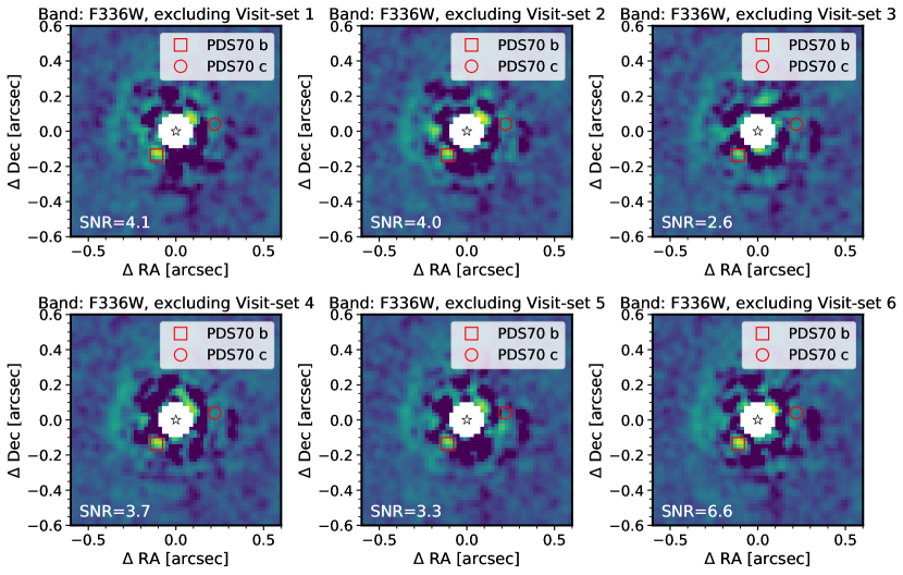
Figure A.1: Primary-subtracted images in F336W. Each image is the combination of five out of six visit-sets of observations. The expected positions of PDS 70 b and c are marked by squares and circles. The detection SNR for PDS 70 b is annotated in each panel. PDS 70 b is detected with SNR$>2.5$ in every case.

To test if the detection is driven by a single (outlier) epoch, we make primary-subtracted images with each visit-set in turn excluded from the final combined image. As shown in Figure A.1, PDS70b is detected in every image with SNR$>2.5$, regardless of which visit-set is excluded. This test result makes it unlikely that the F336W detection is a false positive signal driven by time-dependent systematics or PSF anisotropy.

2. The detection does not rely on the optimization area of the KLIP algorithms. We experiment with various geometries and optimization areas for KLIP. They include circular apertures centered on the planet with various radii and annular sectors with a variety of inner/outer radii and PA spans. The point source at the expected location of PDS70b is consistently detected regardless of the geometry of the optimization region.

3. Injected synthetic PSFs with the same flux densities and separations as PDS 70 b are recovered with similar SNRs to the observed values for PDS 70 b (Figure 2).

4. Similar signals are not present in a PSF-subtracted image of a background star. We apply the data reduction pipeline to a nearby background star in the field of view of our observations. The KLIP parameters and setups are identical to those in subtracting PDS 70 PSFs. The PSF-subtracted images for the background star do not show any point source like signals (Figure A.2).

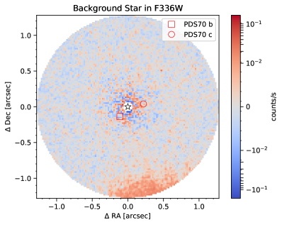
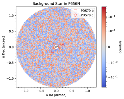
Figure A.2: Primary-subtracted images of a close-by ($2.3\arcsec$) background star. No point-like sources are detected in these images.

5. The location of the detected point source in the F336W band is consistent with the one in the F656N band within $1\sigma$ (Figure 4). They also agree with the expected astrometry for PDS70b estimated from previous studies (e.g., Wang et al., 2020).

Taken together, these five indicators provide strong evidence that the detected point sources are associated with PDS 70 b.

References

- Alcalá et al. (2014) Alcalá, J. M., Natta, A., Manara, C. F., et al. 2014, A&A, 561, A2
- Alcalá et al. (2017) Alcalá, J. M., Manara, C. F., Natta, A., et al. 2017, A&A, 600, A20
- Alencar et al. (2012) Alencar, S. H. P., Bouvier, J., Walter, F. M., et al. 2012, A&A, 541, A116
- Andrews et al. (2018) Andrews, S. M., Huang, J., Pérez, L. M., et al. 2018, ApJ, 869, L41
- Aoyama & Ikoma (2019) Aoyama, Y., & Ikoma, M. 2019, ApJ, 885, L29
- Aoyama et al. (2018) Aoyama, Y., Ikoma, M., & Tanigawa, T. 2018, ApJ, 866, 84
- Aoyama et al. (2020) Aoyama, Y., Marleau, G.-D., Mordasini, C., & Ikoma, M. 2020, arXiv:2011.06608
- Apai et al. (2016) Apai, D., Kasper, M., Skemer, A., et al. 2016, ApJ, 820, 40
- Bae et al. (2019) Bae, J., Zhu, Z., Baruteau, C., et al. 2019, ApJ, 884, L41
- Bailer-Jones et al. (2018) Bailer-Jones, C. A. L., Rybizki, J., Fouesneau, M., Mantelet, G., & Andrae, R. 2018, AJ, 156, 58
- Bellini et al. (2011) Bellini, A., Anderson, J., & Bedin, L. R. 2011, PASP, 123, 622
- Bottom et al. (2017) Bottom, M., Ruane, G., & Mawet, D. 2017, Research Notes of the American Astronomical Society, 1, 30
- Brittain et al. (2020) Brittain, S. D., Najita, J. R., Dong, R., & Zhu, Z. 2020, ApJ, 895, 48
- Calvet & Gullbring (1998) Calvet, N., & Gullbring, E. 1998, ApJ, 509, 802
- Cardelli et al. (1989) Cardelli, J. A., Clayton, G. C., & Mathis, J. S. 1989, ApJ, 345, 245
- Christiaens et al. (2019) Christiaens, V., Cantalloube, F., Casassus, S., et al. 2019, ApJ, 877, L33
- Close (2020) Close, L. M. 2020, AJ, 160, 221
- Dodson-Robinson & Salyk (2011) Dodson-Robinson, S. E., & Salyk, C. 2011, ApJ, 738, 131
- Dong et al. (2015) Dong, R., Zhu, Z., & Whitney, B. 2015, ApJ, 809, 93
- Fang et al. (2009) Fang, M., van Boekel, R., Wang, W., et al. 2009, A&A, 504, 461
- Gaia Collaboration et al. (2016) Gaia Collaboration, Brown, A. G. A., Vallenari, A., et al. 2016, A&A, 595, A2
- Gaia Collaboration et al. (2018) —. 2018, A&A, 616, A1
- Gullbring et al. (1998) Gullbring, E., Hartmann, L., Briceño, C., & Calvet, N. 1998, ApJ, 492, 323
- Haffert et al. (2019) Haffert, S. Y., Bohn, A. J., de Boer, J., et al. 2019, Nat. Astron., 3, 749
- Hartmann et al. (2016) Hartmann, L., Herczeg, G., & Calvet, N. 2016, ARAA, 54, 135
- Hashimoto et al. (2020) Hashimoto, J., Aoyama, Y., Konishi, M., et al. 2020, AJ, 159, 222
- Hashimoto et al. (2012) Hashimoto, J., Dong, R., Kudo, T., et al. 2012, ApJ, 758, L19
- Herczeg et al. (2009) Herczeg, G. J., Cruz, K. L., & Hillenbrand, L. A. 2009, ApJ, 696, 529
- Herczeg & Hillenbrand (2008) Herczeg, G. J., & Hillenbrand, L. A. 2008, ApJ, 681, 594
- Ingleby et al. (2013) Ingleby, L., Calvet, N., Herczeg, G., et al. 2013, ApJ, 767, 112
- Keppler et al. (2018) Keppler, M., Benisty, M., Müller, A., et al. 2018, A&A, 617, A44
- Keppler et al. (2019) Keppler, M., Teague, R., Bae, J., et al. 2019, A&A, 625, A118
- Krist et al. (2011) Krist, J. E., Hook, R. N., & Stoehr, F. 2011, in Society of Photo-Optical Instrumentation Engineers (SPIE) Conference Series, Vol. 8127, Optical Modeling and Performance Predictions V, ed. M. A. Kahan, 81270J
- Lauer (1999) Lauer, T. R. 1999, PASP, 111, 1434
- Liu (2004) Liu, M. C. 2004, Science, 305, 1442
- Marleau et al. (2017) Marleau, G.-D., Klahr, H., Kuiper, R., & Mordasini, C. 2017, ApJ, 836, 221
- Marley et al. (2007) Marley, M. S., Fortney, J. J., Hubickyj, O., Bodenheimer, P., & Lissauer, J. J. 2007, ApJ, 655, 541
- Marois et al. (2006) Marois, C., Lafrenière, D., Doyon, R., Macintosh, B., & Nadeau, D. 2006, ApJ, 641, 556
- Mawet et al. (2014) Mawet, D., Milli, J., Wahhaj, Z., et al. 2014, ApJ, 792, 97
- Mesa et al. (2019) Mesa, D., Keppler, M., Cantalloube, F., et al. 2019, A&A, 632, A25
- Müller et al. (2018) Müller, A., Keppler, M., Henning, T., et al. 2018, A&A, 617, 2
- Muzerolle et al. (1998) Muzerolle, J., Calvet, N., & Hartmann, L. 1998, ApJ, 492, 743
- Muzerolle et al. (2001) Muzerolle, J., Calvet, N., & Hartmann, L. 2001, ApJ, 550, 944
- Natta et al. (2004) Natta, A., Testi, L., Muzerolle, J., et al. 2004, A&A, 424, 603
- Pecaut & Mamajek (2016) Pecaut, M. J., & Mamajek, E. E. 2016, MNRAS, 461, 794
- Pueyo (2016) Pueyo, L. 2016, ApJ, 824, 117
- Rajan et al. (2015) Rajan, A., Barman, T., Soummer, R., et al. 2015, ApJ, 809, L33
- Rigliaco et al. (2012) Rigliaco, E., Natta, A., Testi, L., et al. 2012, A&A, 548, A56
- Sallum et al. (2015) Sallum, S., Follette, K. B., Eisner, J. A., et al. 2015, Nature, 527, 342
- Soummer et al. (2012) Soummer, R., Pueyo, L., & Larkin, J. 2012, ApJ, 755, L28
- Stolker et al. (2020) Stolker, T., Marleau, G.-D., Cugno, G., et al. 2020, A&A, 644, A13
- Szulágyi & Ercolano (2020) Szulágyi, J., & Ercolano, B. 2020, ApJ, 902, 126
- Thanathibodee et al. (2019) Thanathibodee, T., Calvet, N., Bae, J., Muzerolle, J., & Hernández, R. F. 2019, ApJ, 885, 94
- Thanathibodee et al. (2020) Thanathibodee, T., Molina, B., Calvet, N., et al. 2020, ApJ, 892, 81
- Uyama et al. (2021) Uyama, T., Hashimoto, J., Beichman, C. A., et al. 2021, Research Notes of the American Astronomical Society, 5, 9
- Valenti et al. (1993) Valenti, J. A., Basri, G., & Johns, C. M. 1993, AJ, 106, 2024
- Wagner et al. (2018) Wagner, K., Follete, K. B., Close, L. M., et al. 2018, ApJ, 863, L8
- Wang et al. (2020) Wang, J. J., Ginzburg, S., Ren, B., et al. 2020, AJ, 159, 263
- Wang et al. (2021) Wang, J. J., Vigan, A., Lacour, S., et al. 2021, arXiv:2101.04187
- Zhang et al. (2018) Zhang, S., Zhu, Z., Huang, J., et al. 2018, ApJ, 869, L47
- Zhou et al. (2014) Zhou, Y., Herczeg, G. J., Kraus, A. L., Metchev, S., & Cruz, K. L. 2014, ApJ, 783, L17
- Zhu et al. (2011) Zhu, Z., Nelson, R. P., Hartmann, L., Espaillat, C., & Calvet, N. 2011, ApJ, 729, 47
- Zurlo et al. (2020) Zurlo, A., Cugno, G., Montesinos, M., et al. 2020, A&A, 633, A119