The Loudest Stellar Heartbeat: Characterizing the most extreme amplitude heartbeat star system

Abstract

We characterize the extreme heartbeat star system MACHO 80.7443.1718 in the LMC using TESS photometry and spectroscopic observations from the Magellan Inamori Kyocera Echelle (MIKE) and SOAR Goodman spectographs. MACHO 80.7443.1718 was first identified as a heartbeat star system in the All-Sky Automated Survey for SuperNovae (ASAS-SN) with $P_{\rm orb}=32.836\pm 0.008\,{\rm d}$. MACHO 80.7443.1718 is a young (${\sim}6$ Myr), massive binary, composed of a B0 Iae supergiant with $M_{1}\simeq 35M_{\odot}$ and an O9.5V secondary with $M_{2}\simeq 16M_{\odot}$ on an eccentric ($e=0.51\pm 0.03$) orbit. In addition to having the largest variability amplitude amongst all known heartbeats stars, MACHO 80.7443.1718 is also one of the most massive heartbeat stars yet discovered. The B[e] supergiant has Balmer emission lines and permitted/forbidden metallic emission lines associated with a circumstellar disk. The disk rapidly dissipates at periastron which could indicate mass transfer to the secondary, but re-emerges immediately following periastron passage. MACHO 80.7443.1718 also shows tidally excited oscillations at the $N=25$ and $N=41$ orbital harmonics and has a rotational period of 4.4 d.

1 Introduction

Heartbeat stars are binaries with short period ($P\lesssim 1$ yr), eccentric ($e\gtrsim 0.3$) orbits. The light curves of heartbeat stars are defined by oscillations outside of periastron combined with a brief, high amplitude ellipsoidal variations at periastron that gives rise to a unique “heartbeat” signature. Heartbeat stars were first discovered and characterized using data from the Kepler space telescope (Borucki et al., 2010; Thompson et al., 2012; Kirk et al., 2016) and its follow-up mission K2 (Howell et al., 2014). Kepler identified over 170 heartbeat stars (Kirk et al., 2016). The photometric modulations of these systems are dominated by the effects of tidal distortion, reflection and Doppler beaming close to periastron (Kumar et al., 1995; Fuller, 2017). The variability amplitude of most heartbeat stars is very small ($\lesssim 1$ mmag; Kirk et al. 2016; Hambleton et al. 2018).

Heartbeat stars show tidally excited oscillations (TEOs) at exact integer multiples of the orbital frequency (Fuller, 2017) driven by the tidal forcing at periastron. The largest amplitude TEOs are resonances between harmonics of the orbital frequency and the normal mode frequencies of the star (Fuller, 2017; Cheng et al., 2020a). Most known heartbeat stars are relatively low-mass A and F type stars. However, several massive OB-type heartbeat stars have recently been discovered. For example, $\iota$ Ori is a massive heartbeat star system consisting of a O9 III primary and a B1 III-IV companion discovered by BRITE (Pablo et al., 2017) and $\epsilon$ Lupi consists of two early-type main sequence B stars (Pablo et al., 2019). Recently, Kołaczek-Szymański et al. (2021) identified 20 massive heartbeat stars using data from the Transiting Exoplanet Survey Satellite (TESS; Ricker et al. 2015). Heartbeat stars with TEOs are useful laboratories to study equilibrium and dynamical tides (Guo et al., 2020), and massive heartbeat systems can be used to study these processes in the context of binary systems that are the progenitors for compact objects.

MACHO 80.7443.1718 with J2000 coordinates $(\alpha,\delta)=(81.601924^{\circ},-68.784706^{\circ})$, was initially classified as an eclipsing binary in the Large Magellanic Cloud (LMC) with a period of $P{\sim}32.8\;$d by the MACHO survey (Alcock et al., 1997). In our previous work (Jayasinghe et al., 2019b), we identified it as a heartbeat star (ASASSN-V J052624.38-684705.6) using data from The All-Sky Automated Survey for SuperNovae (ASAS-SN, Shappee et al. 2014; Kochanek et al. 2017; Jayasinghe et al. 2018, 2019a) and TESS. MACHO 80.7443.1718 is a massive star that is part of the LH58 OB association in the LMC, northwest of 30 Doradus. An archival spectrum classified it as a B0.5 Ib/II (Garmany et al., 1994), evolved blue star with $U-B=-0.84$ mag, and $B-V=0.11$ mag (Massey, 2002). We found that MACHO 80.7443.1718 displayed the largest known heartbeat flux variations, with a peak-to-peak variability of ${\sim}40\%$ at periastron and oscillation amplitudes of ${\sim}10\%$ due to TEOs outside periastron.

Here we characterize this extreme amplitude heartbeat star using TESS photometry and spectroscopic observations from the Magellan/MIKE and SOAR/Goodman spectrographs. We discuss the TESS observations and spectroscopic followup in Section 2. In Section 3, we characterize the binary orbit, stellar parameters, and TEOs of this binary system. In Section 4, we discuss the implications of our observations of this unique heartbeat star system. We present a summary of our results in Section 5.

2 Observations

2.1 Photometry

MACHO 80.7443.1718 lies in the Southern TESS CVZ which allowed us to extract TESS light curves for both Sectors 1 and 2 in Jayasinghe et al. (2019b). Here, we extend the TESS photometry using data from sectors 1-7, 9-10, 12-13, 27 and 29-34. We analyzed the TESS data using an image subtraction pipeline derived from that used to process ASAS-SN data which has been optimized for use with the TESS FFIs (Vallely et al., 2020). This pipeline is based on the ISIS package (Alard & Lupton, 1998; Alard, 2000), and a detailed description of the TESS-specific corrective procedures can be found in Vallely et al. (2020).

While this pipeline produces excellent differential flux light curves, the large pixel scale of TESS makes it difficult to obtain reliable measurements of the reference flux of a given source. Here we have estimated the reference flux using the ticgen software package (Barclay, 2017; Stassun et al., 2018). The TESS-band magnitude estimates from ticgen were converted into fluxes using an instrumental zero point of 20.44 electrons per second in the FFIs, based on the values provided in the TESS Instrument Handbook. Flux was then added to the raw differential light curves such that the median of each sector’s observations matched the estimated reference value. This allowed us to produce the normalized flux light curves shown in Figure 1. The light curves do not include epochs where the observations were compromised by scattered light artifacts from the Earth or Moon.

From the combined TESS light curve, we derive an orbital period of

$$\rm P_{\rm orb,TESS}=32.8194\pm 0.0105\,{\rm d},$$ (1)

which is consistent with the period of

$$\rm P_{\rm orb}=32.83627\pm 0.00846\,{\rm d},$$ (2)

derived from the ASAS-SN light curve. For the remainder of this work, we adopt the ASAS-SN orbital period. We use the periastron ephemeris derived from the TESS data of,

$$\rm{\rm BJD}_{\rm periastron}=2458373.61518+32.83627\times E\,,$$ (3)

where the epoch $\rm E$ is the number of orbits since the time of minimum. Figure 1 shows the phased TESS light curve for MACHO 80.7443.1718. The strong ellipsoidal variation and TEOs are clearly resolved in the TESS data. Following the photometric maximum, we see significant variations in the descending branch of the ellipsoidal variation signal ($0.05<\Phi<0.15$). The inclusion of the 16 additional TESS sectors significantly improves our previous analysis of the TEOs (see $\S 3.4$).

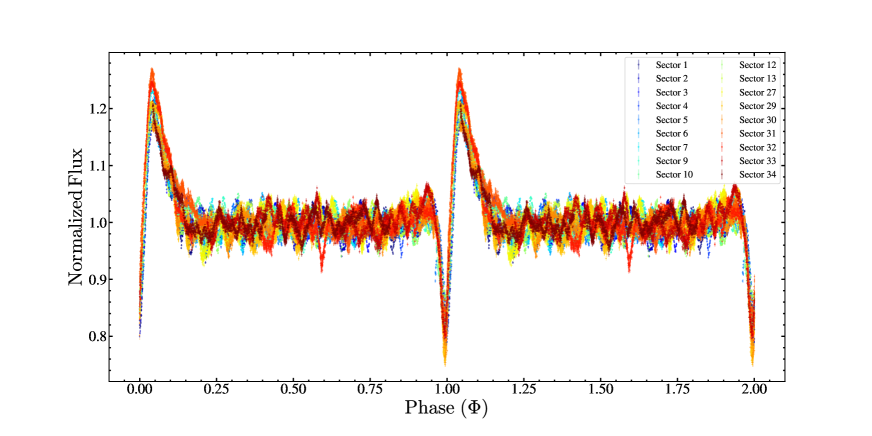
Figure 1: The phased TESS light curve for MACHO 80.7443.1718. The points are colored by the sector.

We also retrieve 23 archival photometric measurements spanning $22.2\mu$m ($W4$) through the $U$-band (Table 1). In addition, we obtained archival Swift UVOT (Roming et al., 2005) images in the $UVW1$ (2600 Å), $UVM2$ (2246 Å), and $UVW2$ (1928 Å) bands (Poole et al., 2008) from the LMC Survey (Hagen et al., 2017) pointings 148 and 16. Each epoch of UVOT data includes 2 observations per filter, which we combined using the uvotimsum package. We then used uvotsource to extract source counts using a 6$\aas@@fstack{\prime\prime}$0 radius aperture centered on the star. We measured the background counts using a source-free region with radius of $\sim$18$\aas@@fstack{\prime\prime}$0. Using the most recent calibrations (Poole et al., 2008; Breeveld et al., 2010), we converted the UVOT counts into fluxes and magnitudes. We combined all 4 epochs with a weighted average and summed the uncertainties on the individual epochs with the standard deviation in quadrature to obtain our error estimate. This photometry is used for the SED models in $\S 3.2$.

Table 1: Multi-band photometry measurements for MACHO 80.7443.1718

Magnitude	$\sigma$	Filter	Reference
14.24	0.04	UVM2	This work
14.22	0.03	UVW2	This work
13.92	0.04	UVW1	This work
12.83	0.10	U	Massey (2002)
12.630	0.038	U	Zaritsky et al. (2004)
13.67	0.10	B	Massey (2002)
13.617	0.106	B	Zaritsky et al. (2004)
13.608	0.262	V	Zaritsky et al. (2004)
13.56	0.10	V	Massey (2002)
13.43	0.10	R	Massey (2002)
13.283	0.079	I	Zaritsky et al. (2004)
13.255	0.007	I	Cioni et al. (2000)
13.020	0.022	J	Cutri et al. (2003)
12.978	0.023	J	Cioni et al. (2000)
12.833	0.022	H	Cutri et al. (2003)
12.734	0.030	$K_{s}$	Cutri et al. (2003)
12.411	0.033	[3.6]	Meixner et al. (2006)
12.300	0.030	[4.5]	Meixner et al. (2006)
12.135	0.067	[5.8]	Meixner et al. (2006)
12.416	0.024	W1	Wright et al. (2010)
12.337	0.022	W2	Wright et al. (2010)
9.901	0.071	W3	Wright et al. (2010)
6.197	0.092	W4	Wright et al. (2010)

2.2 Optical Spectroscopy

We obtained 17 epochs of spectroscopy: 4 with Magellan/MIKE (Bernstein et al., 2003), and 13 with SOAR/Goodman (Clemens et al., 2004), between 2019 Jan 6 and 2019 Aug 6. The first and third MIKE epochs were obtained with a 0$\aas@@fstack{\prime\prime}$7 slit, while the other two epochs used a 1$\aas@@fstack{\prime\prime}$0 slit. The resolution of the spectra in the region of interest (see below) was about 0.12 Å and 0.16 Å, respectively, for the two slit widths. Data were obtained for both the blue and red sides of the instrument; here, only data from the blue camera are used. The MIKE data were reduced using CarPy (Kelson et al., 2000; Kelson, 2003). The SOAR spectra were taken with a 2100 lines mm^-1 grating and a 0$\aas@@fstack{\prime\prime}$95 slit, giving a resolution of 1.0 Å over the wavelength range $\sim 4500$–5170 Å. The exposure time was 1200 s per epoch. The data were reduced and optimally extracted in the standard manner. For both datasets, we report the mid-exposure observation times as Barycentric Julian Dates (BJD) on the TDB system (Eastman et al., 2010). Figure 2 illustrates the SOAR spectra (excluding two epochs with low SNR). We see many emission lines, including the Balmer $\rm H\beta$ line, suggesting that this source is likely a Be star with a circumstellar disk.

In the majority of the spectra, most of the strong absorption lines are contaminated by emission and hence unusable for radial velocities. The strongest line without evidence for emission is the He i line at $4922\textup{\AA}$. For the MIKE spectra, we used this absorption line to determine velocities, using a spectrum of the B1 III star HD 68761 from the UVES POP library (Bagnulo et al., 2003) as a template. For the SOAR data, we used the highest signal-to-noise SOAR spectrum (that of 2019 Mar 24) as a template and obtained radial velocities of the other SOAR spectra through cross-correlation with this template, again in the region of the $4922\textup{\AA}$ line. The velocity of the template was determined through cross-correlation with a spectrum of the bright B0 III star HD 114122 taken with the same instrumental setup. The barycentric radial velocities of all the spectra are given in Table 2. Note that, due to the rapid rotation of the star and the resulting broad lines, the MIKE spectra do not have substantially smaller velocity uncertainties than the SOAR spectra.

Table 2: Radial velocity (RV) measurements for MACHO 80.7443.1718 from SOAR and MIKE.

BJD	Date	Phase ($\Phi)$	RV ($\rm kms^{-1}$)	$\sigma_{RV}$ ($\rm kms^{-1}$)	Instrument
2458489.6195626	2019-01-06	0.533	271.0	5.8	MIKE
2458498.5758614	2019-01-15	0.806	251.3	5.2	MIKE
2458517.5984611	2019-02-03	0.385	294.7	6.2	MIKE
2458491.6776199	2019-01-08	0.595	254.2	9.8	SOAR
2458525.5646330	2019-02-11	0.627	256.2	12.8	SOAR
2458547.5450865	2019-03-05	0.297	301.2	4.9	SOAR
2458567.4966222	2019-03-24	0.905	245.3	4.0	SOAR
2458579.5027003	2019-04-06	0.270	315.2	6.5	MIKE
2458581.4869998	2019-04-07	0.331	306.8	4.5	SOAR
2458582.4874062	2019-04-08	0.361	294.7	4.8	SOAR
2458595.4763313	2019-04-21	0.756	247.8	4.4	SOAR
2458604.4649556	2019-04-30	0.030	350.9	6.9	SOAR
2458607.5096233	2019-05-04	0.123	360.9	7.3	SOAR
2458664.9182869	2019-06-30	0.871	237.0	6.0	SOAR
2458665.8982865	2019-07-01	0.901	252.8	5.3	SOAR
2458693.9235514	2019-07-29	0.755	251.3	6.4	SOAR
2458701.9156224	2019-08-06	0.998	313.8	5.5	SOAR

Figure 2: SOAR spectra for MACHO 80.7443.1718 sorted by the orbital phase $\Phi$, where $\Phi=0$ corresponds to periastron.

3 Results

3.1 Spectral classification

Using a low-resolution spectrum, MACHO 80.7443.1718 was previously classified as a B0.5 Ib/II star by Garmany et al. (1994). As we previously noted in $\S 2$, MACHO 80.7443.1718 is an emission line star with significant continuum emission from a disk that complicates analysis of the spectra. To estimate the spectral type, we calculate the equivalent widths and their ratios in the MIKE spectra for various lines that are typically used to assign spectral types for OB stars (Conti & Alschuler, 1971; Mathys, 1988; Sota et al., 2011, 2014; Martins, 2018). These results are summarized in Table 3.

Based on the classical spectral type criterion for OB stars using the ratio $\rm\text{He\,{i}}\,4471$/$\rm\text{He\,{ii}}\,4542$, MACHO 80.7443.1718 has a spectral type later than O9.5 (Conti & Alschuler, 1971; Mathys, 1988). The ratio $\rm\text{He\,{i}}\,4144$/$\rm\text{He\,{ii}}\,4200=1.66\pm 0.50$ is very similar to O9.7 stars with $\rm\text{He\,{i}}\,4144$/$\rm\text{He\,{ii}}\,4200=1.98\pm 1.00$ (Martins, 2018). The average ratio of $\rm\text{He\,{i}}\,4388$/$\rm\text{He\,{ii}}\,4542=3.37\pm 0.52$ is somewhat different from O9.7 stars ($2.45\pm 0.99$) but falls within the reported dispersion in Martins (2018). The definition of the O9.7 spectral type is based on the ratio $\rm\text{Si\,{iii}}\,\lambda 4552$/$\rm\text{He\,{ii}}\,\lambda 4542{\sim}1.0$ (Sota et al., 2011). However, even though MACHO 80.7443.1718 has $\rm\text{Si\,{iii}}\,\lambda 4552$/$\rm\text{He\,{ii}}\,\lambda 4542{\sim}1.6$, which is larger than this canonical definition, there are a few stars with O9.7 spectral types that have values close to ${\sim}2$ (Martins, 2018). It is also possible that MACHO 80.7443.1718 is an early B0/B0.2 star. Based on this analysis, MACHO 80.7443.1718 likely has a spectral type in the range O9.7–B0.2. Here, we will adopt the B0 spectral type for simplicity.

The luminosity classes of late-O stars can be determined using the ratios $\rm\text{Si\,{iv}}\,4089$/$\rm\text{He\,{i}}\,4026$ and $\rm\text{He\,{ii}}\,4686$/$\rm\text{He\,{i}}\,4713$ which differ significantly for dwarfs and supergiants (Sota et al., 2011, 2014; Martins, 2018). Given the uncertainty in our assigned spectral type, we will utilize these criteria to assign a luminosity class even though MACHO 80.7443.1718 was assigned an early B0 spectral type. MACHO 80.7443.1718 has $\rm\text{Si\,{iv}}\,4089$/$\rm\text{He\,{i}}\,4026=1.20\pm 0.19$ which is most comparable to Ia supergiants that have $\rm\text{Si\,{iv}}\,4089$/$\rm\text{He\,{i}}\,4026=1.07\pm 0.20$ (Martins, 2018). I/Iab stars have $\rm\text{Si\,{iv}}\,4089$/$\rm\text{He\,{i}}\,4026=0.85\pm 0.11$ (Martins, 2018). Similarly, MACHO 80.7443.1718 has $\rm\text{He\,{ii}}\,4686$/$\rm\text{He\,{i}}\,4713=0.12\pm 0.07$ which is again comparable to Ia supergiants with $\rm\text{He\,{ii}}\,4686$/$\rm\text{He\,{i}}\,4713=0.31\pm 0.10$ (Martins, 2018). In comparison, I/Iab stars have $\rm\text{He\,{ii}}\,4686$/$\rm\text{He\,{i}}\,4713=0.90\pm 0.30$ (Martins, 2018).

Based on this analysis, we assign the B0 Iae spectral type to the primary component of this heartbeat star system. Even though the assignment of a spectral type to this system is complicated by spectral variability, continuum emission from the disk, and the contribution of the companion star, our spectral classification does not differ significantly from that of Garmany et al. (1994).

In Figure 3, we compare the MIKE spectrum taken on UT 2019-04-06 ($\Phi=0.270$) with spectra of standard late-O and early-B supergiants. The O-star spectra are obtained from the Galactic O-star catalog (Maíz Apellániz et al., 2013) and the B-star spectra are obtained from Walborn & Fitzpatrick (1990). While there are differences between the spectra, the assigned B0 spectral type is a reasonable match to the templates. Visually, based on the temperature sensitive $\rm\text{Mg\,{ii}}\,4481$ doublet, MACHO 80.7443.1718 should have a spectral type earlier than B1. We measure an average equivalent width of $\rm EW(\text{Mg\,{ii}}\,4481)=57\pm 7\,m\textup{\AA}$ which is consistent with a late-O or early-B spectral type (Lennon, 1997).

Table 3: The average equivalent width ratios and their dispersion calculated using the MIKE spectra.

EW Ratio	Measurement
$\rm\text{He\,{i}}\,\lambda 4471$/$\rm\text{He\,{ii}}\,\lambda 4542$	$5.16\pm 0.71$
$\rm\text{He\,{i}}\,\lambda 4144$/$\rm\text{He\,{ii}}\,\lambda 4200$	$1.66\pm 0.50$
$\rm\text{He\,{i}}\,\lambda 4388$/$\rm\text{He\,{ii}}\,\lambda 4542$	$3.37\pm 0.52$
$\rm\text{He\,{ii}}\,\lambda 4686$/$\rm\text{He\,{i}}\,\lambda 4713$	$0.12\pm 0.07$
$\rm\text{Si\,{iii}}\,\lambda 4552$/$\rm\text{He\,{ii}}\,\lambda 4542$	$1.59\pm 0.18$
$\rm\text{Si\,{iv}}\,\lambda 4089$/$\rm\text{He\,{i}}\,\lambda 4026$	$1.20\pm 0.19$

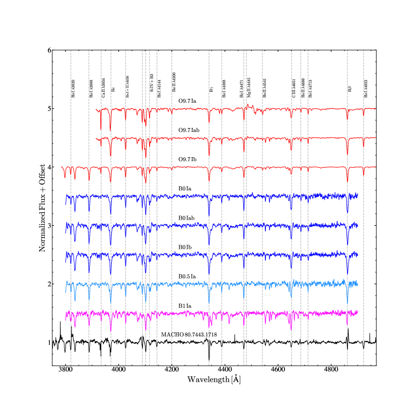
Figure 3: Comparison of various spectral type standards from Maíz Apellániz et al. (2013) and Walborn & Fitzpatrick (1990) with the MIKE spectrum at phase $\Phi=0.270$ (black).

3.2 Stellar Parameters

The absorption lines from the star are broadened, suggesting that it is rapidly rotating. We use the moderate resolution SOAR spectra to measure the projected rotational velocity $v_{\rm rot}\,\textrm{sin}\,i$ in the manner described by Strader et al. (2014) in the region of the 4922 Å line. We convolved the spectrum of the star HD 114122 taken with the same setup with kernels spanning a range of $v_{\rm rot}\,\textrm{sin}\,i$ and assuming a standard limb darkening law. Cross-correlation of the convolved spectra with the original star yields a relation between the input $v_{\rm rot}\,\textrm{sin}\,i$ and the FWHM of the cross-correlation peak. Seven of the SOAR spectra had high enough S/N for this measurement, and we found a final value of $v_{\rm rot}\,\textrm{sin}\,i=174\pm 34$ km s^-1. The uncertainty is the standard deviation of the measurements, which is primarily determined not by the quality of the spectra but by true changes in the shape of the line, perhaps due to a time-variable wind or outflow from the star. Unfortunately, the lack of an appropriate standard star makes it impossible to repeat this analysis for the MIKE spectra. There are indeed variations in the profile of the 4922 Å line in the MIKE spectra, consistent with the findings from the SOAR spectra. From this estimate of $v_{\rm rot}\,\sin(i)$, the radius from the SED (see below) and the orbital inclination $i$ from Jayasinghe et al. (2019b), the rotational velocity of the primary star is $v_{\rm rot}=247\pm 48\,\rm km\,s^{-1}$, which implies a rotation period of $P_{\rm orb}=4.85\pm 1.11$ d.

To estimate the surface temperature ($T_{\rm{eff}}$) and surface gravity ($\log(g)$), we compare the high-resolution MIKE spectra with the TLUSTY OSTAR02 and BSTAR06 model atmospheres at $Z/Z_{\odot}=0.5$ (Lanz & Hubeny, 2003, 2007). The model spectra are convolved using $v\,\textrm{sin}\,i=174$ km s^-1, assuming a standard limb darkening law. We use the BSTAR06 grid for $T_{\rm{eff}}\leq 30000\,K$ and the OSTAR02 grid for $T_{\rm{eff}}>30000\,K$. The BSTAR06 grid extends to $T_{\rm{eff}}=30000\,K$ with a grid spacing of $\rm\Delta T_{eff}=1000\,K$ and $\Delta\log(g)=0.25$. In comparison, the OSTAR02 grid begins at $T_{\rm{eff}}=27500\,K$ with a grid spacing of $\rm\Delta T_{eff}=2500\,K$ and $\Delta\log(g)=0.25$.

To determine $T_{\rm{eff}}$ and $\log(g)$, the MIKE spectra are compared with the model atmospheres at various He i and He ii absorption lines. The best overall fit is returned for a model atmosphere with $T_{\rm{eff}}=30000\,K$ and $\log(g)=3.25$. Figure 4 compares the model atmospheres at a fixed surface gravity of $\log(g)=3.25$ but with various temperatures against the MIKE spectrum at $\Phi=0.806$ for the He lines $\text{He\,{i}}\,\lambda 4922$ and $\text{He\,{ii}}\,\lambda 4200$. We use these lines because they are less affected by emission from the disk. He ii is particularly sensitive to the surface temperature and the observed $\text{He\,{ii}}\,\lambda 4200$ line best agrees with $T_{\rm{eff}}=30000$ K. Higher surface temperatures are clearly incompatible with our observations.

Figure 5 compares the best model atmosphere with $T_{\rm{eff}}=30000\,K$ and $\log(g)=3.25$ to the MIKE spectra of selected He i and He ii absorption lines. There is clear evidence for spectral variability and emission components in the He i lines, particularly the emission component is distinctly seen in the $\text{He\,{i}}\,\lambda 4471$ line. The $\text{He\,{ii}}\,\lambda 4541$ and $\text{He\,{ii}}\,\lambda 4686$ lines are relatively weak compared to the $\text{He\,{ii}}\,\lambda 4200$ line. However, the equivalent width of the $\text{He\,{ii}}\,\lambda 4686$ line grows weaker with increasing luminosity, and is weakest for the Ia luminosity class (Martins, 2018). This is entirely consistent with the B0 Iae spectral type that we assigned previously (see $\S 3.1$).

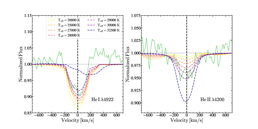
Figure 4: Comparison of various BSTARO6 and OSTAR02 model atmospheres (Lanz & Hubeny, 2003, 2007) at a fixed surface gravity of $\log(g)=3.25$ (dashed lines) against the MIKE spectrum at $\Phi=0.806$ for the $\text{He\,{i}}\,\lambda 4922$ and $\text{He\,{ii}}\,\lambda 4200$ absorption lines. The MIKE spectrum has been smoothed using a Gaussian kernel but not by enough to modify the line profiles.

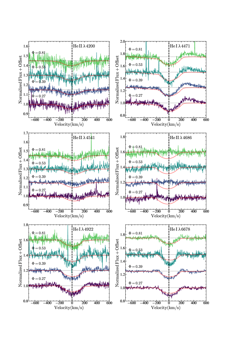
Figure 5: MIKE line profiles for $\text{He\,{ii}}\,\lambda 4200$, $\text{He\,{i}}\,\lambda 4471$, $\text{He\,{ii}}\,\lambda 4541$, $\text{He\,{ii}}\,\lambda 4686$, $\text{He\,{i}}\,\lambda 4922$ and $\text{He\,{i}}\,\lambda 6678$. The TLUSTY BSTAR06 model atmosphere with $T_{\rm{eff}}=30000\,K$ and $\log(g)=3.25$ is shown in red (Lanz & Hubeny, 2003, 2007).

Using the $UBV$ photometry in Table 1, we can derive a photometric temperature using the classical reddening free $Q$ parameter (Johnson, 1958; Bragança et al., 2012), defined as $Q=(U-B)-X(B-V),$ with $X=E(U-B)/E(B-V).$ The $Q$ parameter can then be used to estimate the temperature using the calibration given by Massey et al. (1989),

$$\log({T_{\rm{eff}}})=3.944-0.267Q+0.364Q^{2}.$$ (4)

Using a standard value ($X=0.72$) for the reddening ratio, we obtain $Q=-0.9791$, which implies $\log({T_{\rm{eff}}})=4.554$ and $T_{\rm{eff}}\simeq 36000\,K$. Using a similar method, Massey (2002) estimated a higher temperature of $T_{\rm{eff}}\simeq 39,000$ K for this source. These photometric estimates of the temperature are considerably higher than our spectroscopic estimate, but they are less reliable. The lack of strong He ii absorption lines in the spectra also rule out this higher temperature estimate.

We used DUSTY (Ivezic & Elitzur, 1997; Elitzur & Ivezić, 2001) inside a Markov Chain Monte Carlo wrapper (Adams & Kochanek, 2015) to fit the spectral energy distribution (SED) of MACHO 80.7443.1718 using the 18 photometric measurements spanning $3.6\mu$m thorough the UVM2 band (Table 1). We assumed foreground extinction due to $R_{V}=3.1$ dust (Cardelli et al., 1989) and used Castelli & Kurucz (2003) model atmospheres for the star. Since MACHO 80.7443.1718 is located in the LMC, we assume a distance of $d_{\rm LMC}=50\,\rm kpc$ (Pietrzyński et al., 2013). Assuming minimum luminosity uncertainties of 10% for each band, the fits have $\chi^{2}/N_{dof}\simeq 1$ at fixed $T_{\rm{eff}}$. While these models are adequate for determining the luminosity and extinction at fixed temperature, they are not reliable for determining a temperature (especially since they all lie on the Rayleigh-Jeans side of the SED). For $T_{\rm{eff}}\simeq 30,000$ K, we obtain $\log(L/L_{\odot})=5.61\pm 0.04$ with $E(B-V)\simeq 0.39\pm 0.02$ mag.

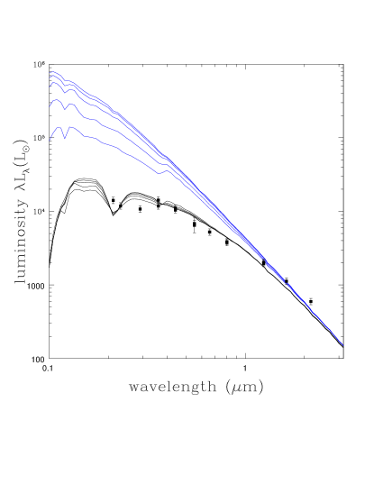
Figure 6: The spectral energy distribution (SED) for MACHO 80.7443.1718. The blue lines show the actual stellar SEDs at various $T_{\rm{eff}}$, and the black lines show these SEDs with reddening.

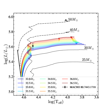
Figure 7: The Hertzsprung-Russell diagram (HRD) for MACHO 80.7443.1718. MIST evolutionary tracks (Choi et al., 2016; Dotter, 2016) are shown for stars at various masses with a metallicity of $\rm[Fe/H]=-0.4$.

With the luminosity and temperature constrained, we can estimate the mass of the primary star using MIST stellar evolutionary tracks (Choi et al., 2016; Dotter, 2016) computed with the Modules for Experiments in Stellar Astrophysics code (MESA, Paxton et al. 2011; Paxton et al. 2013, 2015). We use tracks for stars with a metallicity of $\rm[Fe/H]=-0.4$, which is the average metallicity of the LMC (Choudhury et al., 2016). The position of MACHO 80.7443.1718 in the Hertzsprung-Russell Diagram (HRD) (Figure 7) is consistent with a primary star of mass $M_{1}=34.5^{+1.5}_{-2.0}M_{\odot}$ starting to evolve across the Hertzsprung gap. In the MIST tracks, a $34.5M_{\odot}$ star with $T_{\rm{eff}}\simeq 30,000$ K and $\log(L/L_{\odot})\simeq 5.6$ has $\log(g)=3.2$ which is consistent with the spectroscopic estimate of $\log(g)=3.25\pm 0.25$. Given the luminosity and the temperature, the radius of the primary is $R_{1}=23.7^{+2.9}_{-1.2}M_{\odot}$. For these estimates of the mass and radius, the breakup velocity of the star is ${\sim}530\rm\,km\,s^{-1}$. This implies that MACHO 80.7443.1718 is rotating at $\Omega/\Omega_{\rm crit}{\sim}0.47$.

At its current evolutionary state in the MIST tracks, the age of the primary star is ${\sim}5.8$ Myr. Assuming that MACHO 80.7443.1718 is coeval with the LH58 OB association, we can verify its age by fitting isochrones to the LH58 color-magnitude diagram (CMD) using the photometry from Garmany et al. (1994). We estimate the global extinction towards LH58 by varying $E(B-V)$ to minimize the residuals between main sequence stars and a $1$ Myr MIST isochrone with $\rm[Fe/H]=-0.4$. We do not consider differential extinction to the members of this association. With this we obtain a reddening of $E(B-V)=0.17\pm 0.01$ mag which we then use to de-redden the LH58 photometry. The reddening towards MACHO 80.7443.1718 ($E(B-V)\simeq 0.39\pm 0.02$ mag) is larger than the reddening towards the LH58 association by $\Delta E(B-V){\sim}0.22$ mag, suggesting the presence of circumstellar dust consistent with the estimated age of the star. Figure 8 shows the de-reddened CMD for the LH58 OB association. The CMD is best-fit by an isochrone at ${\sim}5.6$ Myr, which is consistent with the age estimate of the primary from the MIST models (Figure 7). We estimate the age of the LH58 association, and hence the age of MACHO 80.7443.1718 as $5.6^{+1.5}_{-1.1}$ Myr.

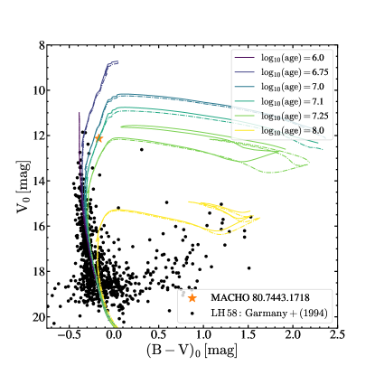
Figure 8: The de-reddened color-magnitude diagram for the LH58 OB association. MIST isochrones (Choi et al., 2016; Dotter, 2016) are shown for populations with a metallicity of $\rm[Fe/H]=-0.4$.

3.3 Binary solution

Previously, we used the analytical model from Kumar et al. (1995) (their Equation 44) to model the flux variations produced by the tidal distortions at periastron (Jayasinghe et al., 2019b). This model has been used to fit the light curves of other heartbeat stars (Thompson et al., 2012). The fit returns the true anomaly, $\phi(t)$, the angle of periastron, $\omega$, the orbital inclination, $i$ and the eccentricity, $e$ as parameters. We attempted fitting a standard eclipsing binary model including irradiation and reflection effects using PHOEBE 2.3 (Prša et al., 2016; Horvat et al., 2018) but were unable to replicate the observed variability amplitude. To accurately model the photometric variability of this unique system, the circumstellar disk will also need to be considered in addition to modeling the dynamical tidal interactions and the two stellar components. We refit the combined TESS light curve with the Kumar et al. (1995) analytical model using the Monte Carlo Markov Chain sampler (MCMC) emcee (Foreman-Mackey et al., 2013). We obtain results that are consistent with our previous model (see Jayasinghe et al. 2019b) with $i=43.9\degree\pm 0.2\degree$, $e=0.565\pm 0.002$ and $\omega=298.2\degree\pm 1.0\degree$. Hereafter, we will use the orbital inclination from the updated fit.

We fit eccentric Keplerian models to the radial velocities using the custom Monte Carlo sampler TheJoker (Price-Whelan et al., 2017). Since the time span of the radial velocities is much shorter than the photometry, the orbital period is not left as a free parameter. Instead, we use a prior to constrain the period by the photometric estimate in Equation 2 ($P=32.8363\pm 0.0085$ d). Leaving the rest of the parameters free, we find a BJD time of periastron $T_{P}=2458505.595\pm 0.301$ d, eccentricity $e=0.506\pm 0.033$, argument of periastron $\omega=302.1\pm 5.1^{\degree}$, semi-amplitude $K_{1}=62.9\pm 4.0$ km s^-1, and systemic velocity $\gamma=289.6\pm 1.5$ km s^-1. There are no significant correlations between the variables except for the expected correlation between $T_{P}$ and $\omega$. This fit has a $\chi^{2}=10.0$ for 12 d.o.f. and an rms residual of 4.6 km s^-1, and so is a good fit to the data.

Fitting the TESS photometry gives an independent estimate of $T_{P}$ (Jayasinghe et al., 2019b). This TESS value, extrapolated with the appropriate uncertainty to the first value within the time range of our velocities, is $T_{P}=2458505.470\pm 0.034$ d. This is entirely consistent with the radial velocity-only measurement of $T_{P}$, but more precise. If we re-fit the eccentric model with this estimate as a constraint, the values are very similar: $e=0.507\pm 0.033$, $\omega=300.2\pm 2.0^{\degree}$, $K_{1}=61.9\pm 2.8$ km s^-1, and $\gamma=289.4\pm 1.5$ km s^-1. The goodness of fit is nearly identical at $\chi^{2}=10.3$ for 13 d.o.f. and an rms of 4.7 km s^-1. This fit is shown in Figure 9. We adopt these parameters as our final spectroscopic model. The value for $\omega$ derived from the radial velocities is entirely consistent with the photometric estimate to $<1\sigma$. The eccentricity derived from the radial velocities is slightly smaller (${\sim}1.8\sigma$) than that obtained from the fit to the light curve.

Using the posterior samples, the binary mass function is

$$f(M)=\frac{P_{\rm orb}K_{1}^{3}(1-e^{2})^{3/2}}{(2\pi G)}=0.51^{+0.07}_{-0.06}M_{\odot}$$ (5)

Using this value of $f(M)$, $M_{1}=34.5^{+1.5}_{-2.0}M_{\odot}$ and an inclination angle $i=43.9\pm 0.2\degree$ from the heartbeat model, we find that the mass of the secondary is $M_{2}=15.7\pm 1.3M_{\odot}$.

Figure 10 illustrates the mass of the companion as a function of the mass of the primary. Even for an edge-on orbit, the minimum mass of the companion is $M_{2}\simeq 10M_{\odot}$. The primary is well within its Roche radius ($R_{L}\simeq 71~{}R_{\odot}\simeq 3.0~{}R_{*})$, but at periastron, it approaches Roche Lobe overflow with a fillout factor $f=R_{*}/R_{L,\rm~{}peri}\simeq 0.7$. We do not see strong evidence for a secondary star in our spectra.

To obtain estimates of the stellar parameters of the secondary star, we use the MIST single star models assuming that the secondary is coeval with the primary. While these models do not account for binary interactions, they can provide a useful estimate of the properties of the unseen secondary star. The MIST models suggest that the secondary star has a similar temperature to the primary, with $T_{\rm{eff}}{\sim}31600\pm$ K. Unlike the primary, the secondary star should be on the main sequence with $\log(g)=4.1\pm 0.1$. The MIST models indicate that the secondary has ${\sim}7\%$ of the primary’s luminosity. Given that the secondary has a similar effective temperature and a considerably lower luminosity than the primary, it is challenging to recover the properties of the secondary star from the spectra. Using the calibrations from Martins et al. (2005) for main sequence stars, the secondary star should have an O9.5 spectral type. We will adopt this spectral type and the stellar properties from the MIST models for the secondary. The binary and stellar properties for MACHO 80.7443.1718 are summarized in Table 4.

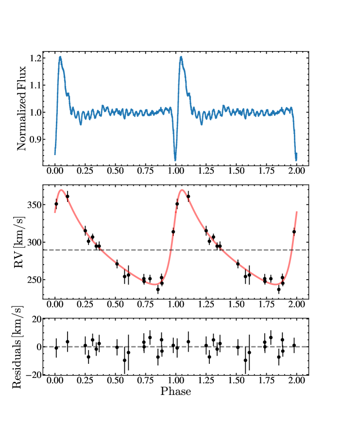
Figure 9: The best fitting Keplerian model to the radial velocity data (red line) for MACHO 80.7443.1718 (middle) compared to the averaged TESS light curve (top). The bottom panel shows the velocity residuals.

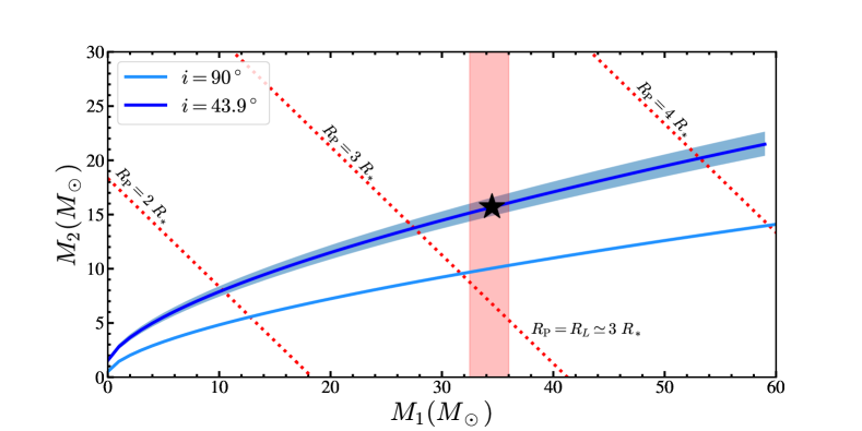
Figure 10: The mass of the companion ($M_{2}$) as a function of the mass of the primary ($M_{1}$). The binary mass function at inclinations of $i=90\degree$ and $43.9\degree$ are shown as the solid lines. Where the periastron distances would correspond to $R_{P}=2~{}R_{*},~{}3~{}R_{*},~{}4~{}R_{*}$ and the Roche Radius ($R_{L}\simeq 3~{}R_{*}$) are shown by the dotted lines. The derived values for $M_{1}$ and $M_{2}$ are illustrated as the black star and the uncertainty in the mass of the primary star and the binary mass function are shaded.

Table 4: Fundamental Parameters for MACHO 80.7443.1718

	Parameter	Primary	Secondary	Reference
	$P_{\rm orb}(d)$	$32.83627\pm 0.00846$		Jayasinghe et al. (2019b)
	$T_{P}(\rm{HJD}-2450000)$	$8505.470\pm 0.034$		Jayasinghe et al. (2019b)
	$i~{}(^{\circ})$	$43.9\pm 0.2$		This work
	$\omega~{}(^{\circ})$	$300.2\pm 2.0$		This work
	$e$	$0.507\pm 0.033$		This work
	${\gamma}~{}(\rm kms^{-1})$	$289.4\pm 1.5$		This work
	$K~{}(\rm kms^{-1})$	$61.9\pm 2.8$	–	This work
	$f(M)~{}(M_{\odot})$	$0.51^{+0.07}_{-0.06}$		This work
	$v\,\sin(i)~{}(\rm kms^{-1})$	$174\pm 34$	–	This work
	$T_{\rm{eff}}~{}(K)$	$30000\pm 1000$	$31600\pm 1000$	This work
	$\log(L/L_{\odot})$	$5.61\pm 0.04$	$4.46^{+0.11}_{-0.12}$	This work
	$\log(g)$	$3.25\pm 0.25$	$4.1\pm 0.1$	This work
	$R~{}(R_{\odot})$	$23.7_{-1.2}^{+2.9}R_{\odot}$	$5.7_{-0.5}^{+0.4}R_{\odot}$	This work
	$M~{}(M_{\odot})$	$34.5_{-2.0}^{+1.5}M_{\odot}$	$15.7\pm 1.3$	This work
	$\rm[Fe/H]$	$-0.4$ (Fixed)		This work
	Spectral Type	B0 Iae	O9.5 V	This work
	Age (Myr)	$5.6_{-1.1}^{+1.5}$		This work
	$E(B-V)$ (mag)	$0.39\pm 0.02$		This work

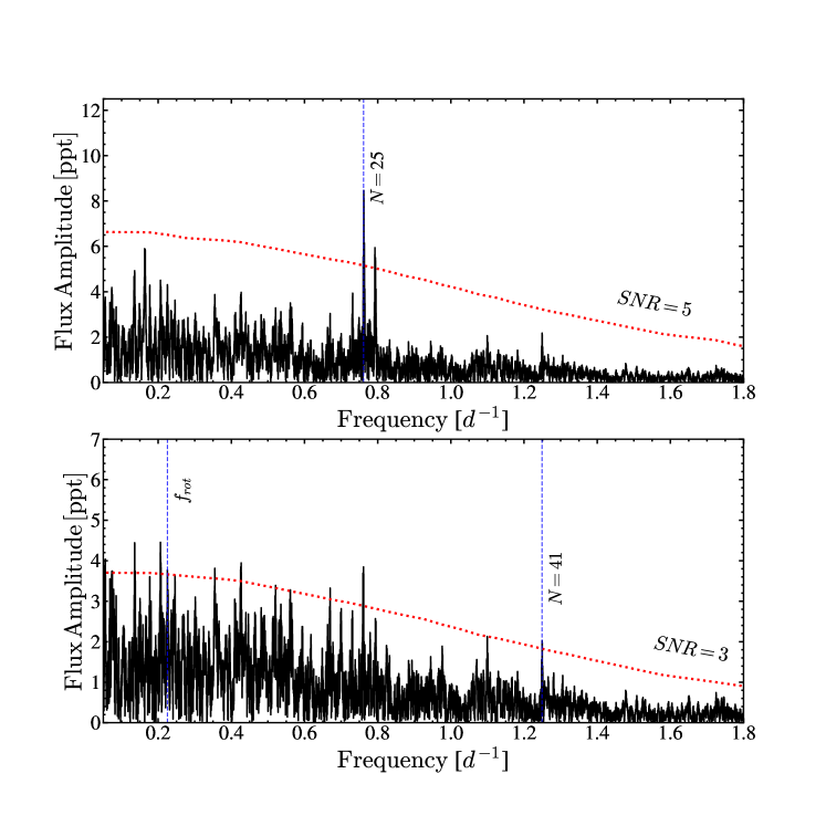
Figure 11: FFT power spectrum of the combined TESS light curve before (top) and after (bottom) subtracting the dominant TEO at $N=25$. The red dashed lines show the flux amplitudes at which $SNR=5$ (top) and $SNR=3$ (bottom) as a function of frequency. The frequencies identified in our analysis are shown in blue.

3.4 Tidally Excited Oscillations

Table 5: Frequencies for MACHO 80.7443.1718, phased to periastron calculated using the multi-sector TESS lightcurve. The errors in frequency, amplitude and phase are calculated through a Monte Carlo analysis.

Type	Frequency $\nu$ ($d^{-1}$)	Orbital Harmonic $N$	$\nu/N\nu_{\rm orb}$	Amplitude (ppt)	Phase	SNR
TEOs
	$0.76207\pm 0.00001$	25	1.0009	$8.4\pm 0.2$	$0.251\pm 0.003$	8.2
	$1.24944\pm 0.00004$	41	1.0007	$2.0\pm 0.2$	$0.969\pm 0.014$	3.3
Rotation
	$0.22530\pm 0.00119$	–	–	$4.4\pm 0.8$	$0.254\pm 0.069$	3.5

Previously, we analyzed both the ASAS-SN and TESS light curves for tidally excited oscillations (TEOs). In both the ASAS-SN and TESS data, we identified a TEO corresponding to the $N=25$ orbital harmonic Jayasinghe et al. (2019b). We also recovered a possible TEO at $N=8$ and $N=7$ in the ASAS-SN and TESS data respectively. However, due to the limited baseline of the TESS data (2 sectors) in our previous work, the resolution of the peaks in the Fast Fourier Transform (FFT) spectrum was poor. Here, we use all 18 sectors of TESS data to analyze the FFT power spectrum for MACHO 80.7443.1718.

We search for TEOs in the TESS data using only the orbital phases $0.25\leq\Phi\leq 0.85$ by calculating the FFT using the Period04 software package (Lenz & Breger, 2005). We iteratively whitened the light curves by fitting sinusoids using the dominant frequency. Peaks with signal-to-noise ratios ($\rm SNRs$) $>3$ were retained. Table 5 lists the frequencies that were retrieved from this analysis of the TESS data. The frequencies were optimized to reduce the light curve residuals and the uncertainties were determined using a Monte Carlo analysis within Period04. The TEO at the $N=25$ mode was the dominant frequency ($P=1.312$ d) with $\rm SNR=8.2$. Figure 11 illustrates the FFT power spectrum before and after subtracting the dominant TEO at $N=25$. Modes corresponding to the $N=22,\,23,\,24,\,26$ and $27$ orbital harmonics are also seen in the power spectrum prior to the subtraction of the TEO at $N=25$, but are not significant after the light curve is whitened.

We identify two other modes in the FFT analysis at $P=4.438$ d and $P=0.800$ d. The latter mode corresponds to a TEO at the $N=41$ orbital harmonic, however the peak at $P=4.438$ d is significantly (${\sim}40\%$) different from the nearest orbital harmonic. A similar frequency was also recovered from the ASAS-SN and TESS data in Jayasinghe et al. (2019b) with $P=4.148$ d and $P=4.621$ d, which we previously attributed to a TEO. However, this mode is very similar to the predicted orbital period of the primary star ($P_{\rm orb}=4.85\pm 1.11$ d) that we estimated from the measurement of $v_{\rm rot}\,\textrm{sin}\,i$ in $\S 3.2$, and is unlikely to be a TEO given its significant deviation from the nearest TEO. This period implies that $v_{\rm rot}\,\textrm{sin}\,i=188\pm 23$ km s^-1 assuming the radius from the SED fit ($\S 3.2$) and the orbital inclination from the heartbeat model ($\S 3.3$), which is consistent with the spectroscopic estimate ($v_{\rm rot}\,\textrm{sin}\,i=174\pm 34$ km s^-1). Studies of the photometric variability in Be stars have noted that periodic variability longward of 2 days could correspond to the beating of non-radial pulsation modes, stellar rotation, Rossby modes or circumstellar activity (Sterken et al., 1996; Labadie-Bartz et al., 2017). The position of MACHO 80.7443.1718 in the HRD (Figure 7), and the period at $P=4.438$ d rules out pulsations (Miglio et al., 2007). Given that this mode is within ${\sim}8\%$ of the expected rotational period of the primary, we believe that this signal originates due to the rotation of the star.

We attempt to identify the pulsation modes corresponding to the $N=25$ and $N=41$ TEOs using tidal theory and models of stellar structure (see for, e.g., Fuller 2017; Guo et al. 2020; Cheng et al. 2020b). Assuming that the TEOs are adiabatic and are standing waves that are not fine-tuned, Guo et al. (2020) approximates the pulsation phases for the dominant $l=2$ modes in heartbeat stars as

$$\phi_{l=2,m}=\left\{\begin{array}[]{rcl}0.25+m\phi_{0}&&{\textrm{if}\ m=2\ \ \textrm{or}-2}\\ 0.25&&{\textrm{if}\ m=0}\end{array}\right.$$ (6)

where $\phi_{0}=0.25-\omega/2\pi$ is the observer’s longitudinal coordinate and $m$ is the mode azimuthal number. These phases are defined with respect to the time of periastron ($\phi=0$). In the case of MACHO 80.7443.1718, $\phi_{0}\simeq-0.58$. The retrograde ($m=2$) or prograde ($m=-2$) modes have a 180$\degree$ phase ambiguity, thus a 0.5 phase offset can be added or subtracted from Equation 6. Therefore, the $m=|2|$ modes can have $\phi\simeq 0.41$ or $\phi\simeq 0.92$. For the $N=25$ TEO we found $\phi\simeq 0.25$, which is entirely consistent with the $m=0$ mode ($\phi=0.25$). The $N=41$ TEO has $\phi\simeq 1$, which is consistent with the $m=|2|$ mode. The phase deviation for the $N=41$ TEO $\Delta\phi(m=|2|)\simeq 0.05$, can occur due to the non-adiabicity of the pulsations and spin-orbit misalignments (Guo et al., 2020).

We also attempted to track the changes in amplitude and phase for the three frequencies in Table 5 across the periastron passages in the TESS data. Once it became clear that simple models of the oscillations would not work, we did not pursue this further. It would be interesting however, to look for variations in the individual modes across periastron passages.

3.5 The B[e] phenomenon

The presence of emission lines in both the SOAR and MIKE spectra suggest that MACHO 80.7443.1718 contains a circumstellar disk. This phenomenon is commonly associated with the classical Be stars (Rivinius et al., 2013). Classical Be stars are rapidly rotating main-sequence B stars that form a Keplerian “decretion” disk (Rivinius et al., 2013). However, this phenomenon also extends to supergiants like MACHO 80.7443.1718 (Kraus, 2019). B[e] supergiants have early B spectral types and show strong Balmer emission alongside narrow emission lines from both permitted and forbidden transitions (Kraus et al., 2010; Kraus, 2019). B[e] supergiants (hereafter B[e] SGs) in the Magellanic Clouds typically have luminosities in the range $\log(L/L_{\odot}){\sim}4.0-6.0$ and have excesses in the near-infrared (NIR) caused by hot ${\sim}1000$ K dust (Lamers et al., 1998; Zickgraf, 2006). B[e] SG winds have a hot, fast line-driven polar component alongside a cool, slow, equatorial component from which forbidden emission lines (for e.g., [O i] and [Fe ii] lines) originate (Lamers et al., 1998; Zickgraf, 2006; Kraus, 2019).

The Balmer line profiles of MACHO 80.7443.1718 show evidence of disk formation and disruption coinciding with the binary orbit. Figure 12 shows the $\rm H\beta$ line profiles in the SOAR spectra as a function of orbital phase. The typical Gaussian $FWHM$ of the $\rm H\beta$ line is ${\sim}675\,\rm km\,s^{-1}$. $\rm H\beta$ emission is typically produced close to the star, at a few $R_{*}$ (Negueruela et al., 2000). Close to periastron ($\Phi=0.030$), we see little evidence of a disk, with $\rm H\beta$ in absorption and very little emission. In the span of ${\sim}4$ days ($\Phi=0.123$), the $\rm H\beta$ line profile evolves into a double-peaked line profile. Be outbursts occur due to mass outflows from the stellar surface to the circumstellar disk (Labadie-Bartz et al., 2017). At the intermediate orbital phases where TEOs dominate ($0.25\leq\Phi\leq 0.85$), the $\rm H\beta$ line profile shows deep shell absorption with emission wings. At late phases, before periastron passage ($\Phi>0.85$), the shell-like line profile evolves to show emission, although the emission is weaker than that seen right after periastron.

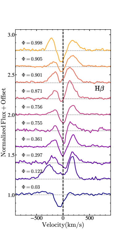
Figure 12: SOAR $\rm H\beta$ line profiles for MACHO 80.7443.1718 sorted by orbital phase.

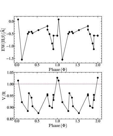
Figure 13: The equivalent width of the $\rm H\beta$ line (top) and the V/R ratio (bottom) as a function of orbital phase $\Phi$.

The violet-to-red ($V/R$) ratio of the double-peaked emission lines is a useful quantity to study Be star emission lines (Mennickent & Vogt, 1991). The violet ($V$) peak dominates when material approaches the observer whereas the red ($R$) peak dominates when material moves away from the observer. Variations in the $V/R$ ratio are related to the dynamics of the cirumstellar disk which include global disk oscillations (Labadie-Bartz et al., 2017). Figure 13 shows the evolution of the $V/R$ ratio and the equivalent widths ($\rm EW(H\beta)$) of the $\rm H\beta$ line profiles with the orbital phase. This system shows significant $V/R$ variability. At periastron, the $\rm H\beta$ symmetry is $V>R$, which immediately reverses to $V<R$ within $\Delta\Phi{\sim}0.2$. The equivalent width appears to be correlated with the orbital phase, and suggests that the system undergoes significant outbursts immediately before ($\Phi{\sim}0.9$) and after ($\Phi{\sim}0.1$) approaching periastron. At the intermediate orbital phases ($0.25\leq\Phi\leq 0.85$), the equivalent widths are mostly similar.

Figure 14 shows the TESS photometry and the SOAR $\rm H\beta$ line profiles at $\Phi=0.030$ and $\Phi=0.123$ corresponding to periastron passage and the first spectroscopic epoch with evidence of a circumstellar disk respectively. When compared to a model of the tidal distortions at periastron (Kumar et al., 1995), the TESS light curve shows photometric evidence of outbursts occurring immediately following periastron while the star is tidally deformed. In fact, the scatter in the TESS light curve beyond $\Phi{\sim}0.05$ suggests that the circumstellar disk might form earlier than $\Phi=0.123$. The TEOs following periastron passage likely contribute to mass loss and disk formation.

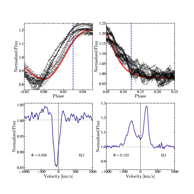
Figure 14: The TESS light curves (top) and SOAR $\rm H\beta$ line profiles (bottom) at $\Phi=0.030$ and $\Phi=0.123$ (vertical lines in top panels) corresponding to periastron passage and the first spectroscopic epoch with evidence of a circumstellar disk. The Kumar et al. (1995) model for tidal distortions at periastron is shown in red.

Figure 15 shows the Balmer line profiles in the high-resolution MIKE spectra as a function of orbital phase. There is clear evidence for strong $\rm H\alpha$ emission. Previous studies of Be stars have shown that $H\alpha$ emission probes a region up to ${\sim}10R_{*}$ (Hummel & Vrancken, 1995; Quirrenbach et al., 1997). The Gaussian $FWHM$ of the $\rm H\alpha$ line is ${\sim}620\,\rm km\,s^{-1}$ and its equivalent width $\rm EW(H\alpha)$ varies from ${\sim}14-26$ Å. The $\rm H\alpha$ line profile is complex, with numerous sharp absorption/emission components that vary with orbital phase. The MIKE $\rm H\beta$ line profiles are comparable to those obtained from SOAR and show shell absorption alongside emission wings at intermediary orbital phases.

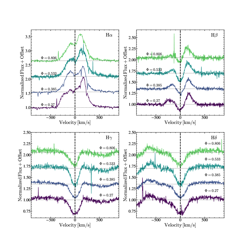
Figure 15: MIKE line profiles for $\rm H\alpha$, $\rm H\beta$, $\rm H\gamma$ and $\rm H\delta$ sorted by phase.

To confirm the B[e] classification, we search for the presence of forbidden emission lines in the high-resolution MIKE spectra, focusing on the [O i] and [Fe ii] lines (Figure 16). Forbidden emission lines are optically thin and collisionally excited. We do not see evidence for [O i] emission lines in the two MIKE spectra at $\Phi=0.270$ and $\Phi=0.385$. We note the presence of the $[\text{O\,{i}}]\,\lambda 6300$ line (single-peaked) at $\Phi=0.533$, but not at $\Phi=0.806$. Compared to the radial velocity of the primary, the $[\text{O\,{i}}]\,\lambda 6300$ line has a radial velocity of ${\sim}+15\rm km\,s^{-1}$ and a Gaussian $FWHM$ of ${\sim}46\,\rm km\,s^{-1}$. In contrast, the $[\text{O\,{i}}]\,\lambda 5577$ line (single-peaked) is only seen at $\Phi=0.806$. The $[\text{O\,{i}}]\,\lambda 5577$ line has a radial velocity of ${\sim}+130\,\rm km\,s^{-1}$ and a Gaussian $FWHM$ of ${\sim}28\,\rm km\,s^{-1}$. Even though the $[\text{O\,{i}}]\,\lambda 6300$ and $[\text{O\,{i}}]\,\lambda 6364$ lines originate from similar regions in terms of temperature and density (Kraus et al., 2010), we do not see the presence of the $[\text{O\,{i}}]\,\lambda 6364$ line in any of our MIKE spectra. There are more emission lines at $\Phi=0.533$ than at $\Phi=0.806$. Here, we also see evidence for single-peaked permitted Fe ii and C i and forbidden [Fe ii] lines in the MIKE spectra. For example, the forbidden $[\text{Fe\,{ii}}]\,\lambda 5269$ line at ${\sim}~{}+185\rm km\,s^{-1}$ has a Gaussian $FWHM$ of ${\sim}24\,\rm km\,s^{-1}$. In contrast, the permitted $\text{Fe\,{ii}}\,\lambda 5265$ line at ${\sim}+195\rm km\,s^{-1}$ has a Gaussian $FWHM$ of ${\sim}11\,\rm km\,s^{-1}$.

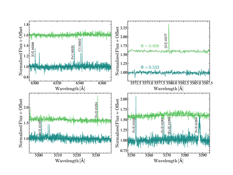
Figure 16: MIKE spectra at $\Phi=0.533$ and $\Phi=0.806$ indicating the presence of O i, C i, Fe ii, [O i] and [Fe ii] emission lines.

3.6 Limit on X-rays

Taken simultaneously with the Swift UVOT observations presented in Section 2.1, MACHO 80.7443.1718 was also observed using the Swift X-ray Telescope (XRT Burrows et al., 2005). To place constraints on the presence of X-ray emission associated with this source, we reprocessed observations sw0045437001-002 and sw0045569001-002 using the Swift xrtpipeline version 0.13.2 and standard filter and screening criteria. Using a 30 arcsec source region centered on MACHO 80.7443.1718 and a 150 arcsec source-free background region located at $(\alpha_{J2000},\delta_{J2000})$=(05:25:30.6787,-68:48:28.700), we find no significant X-ray emission arising from the source. To place deep constraints on the presence of X-ray emission, we combined all four observations using xselect version 2.4k. In this merged dataset, we derive a 3$\sigma$ upperlimit on the 0.3-2.0 keV count rate of $2.0\times 10^{-3}$. Assuming $E(B-V)=0.17$ from Section 3.2, and using the relation from (Liszt, 2014), the Galactic column density towards MACHO 80.7443.1718 is $N_{H}\sim 1.41\times 10^{21}$ cm^-2, which is consistent with the Galactic column density along the line of sight ($N_{H,LOS}=1.44\times 10^{21}$ cm^-2, HI4PI Collaboration et al. 2016). Assuming an absorbed powerlaw with a photon index of 2, we derive absorbed (unabsorbed) flux of $5.0\times 10^{-14}$ erg cm^-2 s^-1 ($8.4\times 10^{-14}$ erg cm^-2 s^-1), which corresponds to an absorbed (unabsorbed) X-ray luminosity of $1.5\times 10^{34}$ erg s^-1 ($2.5\times 10^{34}$ erg s^-1).

4 Discussion

MACHO 80.7443.1718 is by far the most extreme heartbeat discovered. In this work, we have shown that it is also one of the most massive heartbeat star systems thus known with a total mass of $M_{\rm tot}\sim 50~{}M_{\odot}$. We note that Kołaczek-Szymański et al. (2021) discovered that the likely hierarchical quadruple system HD 5980 in the Small Magellanic Cloud with $M_{\rm tot}\gtrsim 150~{}M_{\odot}$ contained a heartbeat star, making this the most massive heartbeat star system known. In comparison, $\iota$ Ori, which consists of a binary system with a O9 III primary and a B1 III-IV secondary has a total mass of $M_{\rm tot}\sim 37~{}M_{\odot}$ (Pablo et al., 2017). $\epsilon$ Lupi is another massive heartbeat star system composed of two early-type main sequence B stars with $M_{\rm tot}\sim 20~{}M_{\odot}$ (Pablo et al., 2019). MACHO 80.7443.1718 is also the only confirmed heartbeat star system consisting of a blue supergiant with a circumstellar disk.

We can understand the short disk lifetime with analytical arguments. The orbital semi-major axis from the period and Kepler’s third law in terms of the stellar radius $R_{*}\simeq 24R_{\odot}$ is

$$a=71R_{\odot}\left({M_{1}+M_{2}\over 10M_{\odot}}\right)^{1/2}\simeq 159R_{\odot}\simeq 6.7R_{*}$$ (7)

where $M_{1}\simeq 34.5M_{\odot}$ and $M_{2}\simeq 15.7M_{\odot}$. The pericentric radius $R_{p}=a(1-e)$ is,

$$R_{p}\simeq 35R_{\odot}\left({M_{1}+M_{2}\over 10M_{\odot}}\right)^{1/2}\simeq 78R_{\odot}\simeq 3.3R_{*}.$$ (8)

For $q=M_{1}/M_{2}\simeq 2.2$, $R_{L}/a=0.448$, and the Roche limit is $R_{L}\simeq 71R_{\odot}\simeq 3.0R_{*},$ (Eggleton, 1983). At periastron, the primary comes close to filling its Roche lobe ($R_{L,\rm~{}peri}\simeq 1.5~{}R_{*}$) with a fillout factor $f=R_{*}/R_{L,\rm~{}peri}\simeq 0.7$. Material in a disk around the primary star will extend beyond the stellar photosphere and so, we should not be surprised to see mass transfer from the disk to the secondary star.

We can use the $\rm H\beta$ line to derive the radius of the $\rm H\beta$ emitting region using the estimate of

$${R_{\beta}\over R_{*}}{\simeq}\left(v\sin(i)v_{\rm crit}\over 350\Delta\lambda\right)^{j}{\simeq}\left(261\over\Delta\lambda\right),$$ (9)

from Mennickent & Vogt (1991), where $v_{\rm crit}{\sim}530\rm\,km\,s^{-1}$, $\Delta\lambda$ is the half-peak separation in the $\rm H\beta$ line profile and $j\approx 1$ is a rotation exponent. While it is not the true radius of the disk, $R_{\beta}$ can track its evolution with orbital phase. $R_{\beta}$ evolves from ${\sim}1.2\,R_{*}$ at $\Phi=0.123$, to ${\sim}2\,R_{*}$ at $\Phi=0.871$, indicating the growth of the disk after periastron passage. In the spectra taken before periastron at $\Phi=0.905$ and at $\Phi=0.998$, this drops to $R_{\beta}\sim 1.4\,R_{*}$, which suggests that the disk starts to shrink as the two stars approach each other. $\rm H\beta$ is in emission at $\Phi=0.998$ but at $\Phi=0.030$, $\rm H\beta$ is in absorption and shows little evidence for a disk (see Figure 12). Thus, in the span of ${\sim}4$ hours the disk around MACHO 80.7443.1718 appears to dissipate. At periastron, a disk beyond a radius $R_{d}>R_{L,\rm~{}peri}\simeq 1.5R_{*}$ will result in mass transfer to the secondary. Given that the disks around Be stars are larger than a few $R_{*}$, it is very likely that mass transfer occurs at periastron in this system. However, this framework is complicated by the tidal interactions exerted on the disk by the secondary.

To obtain a rough estimate of the stability of the disk during a pericentric passage, we used the approach of Kochanek (1993). We set up the stars at apocenter with their nominal masses, put a ring of test particles in circular orbits around the Be star, and then followed their evolution through one orbit. As a simple metric for the stability of the disk as a function of radius, we simply examined the maximum and minimum radii of the test particles at the end and the fraction still bound to the Be star. Material closer than $30R_{\odot}$ likely can remain in a disk. For example, at $30R_{\odot}$ ring ends up with a radial spread of $19.8$ to $36.4R_{\odot}$ with all particles bound. At $25R_{\odot}$ the radial range shrinks to $22.6$ to $26.6R_{\odot}$. At $35R_{\odot}$, the particles are still bound but the radial range has expanded to $4.6$ to $47.4R_{\odot}$. More distant rings are significantly disrupted. At $40$ and $45R_{\odot}$, the outer radius is $\sim 280R_{\odot}$ and the bound fractions are 83% and 72%, respectively. While crude, this experiment suggests that only the very inner portions of the disk can survive a pericentric encounter.

Be stars in eccentric binaries can actually have increased mass loss rates due to binary interactions. At periastron, the secondary component can trigger outbursts in the Be star due to tidal forces that depend on the stellar properties of the Be star and the configuration of the binary orbit (Labadie-Bartz et al., 2017). The role of binary interactions in triggering Be outbursts have been studied with the Be star $\delta$ Sco which is in a highly eccentric ($e=0.94\pm 0.01$) orbit with $P_{\rm orb}\sim 10.6$ years (Miroshnichenko et al., 2003). Spectroscopic observations of $\delta$ Sco at periastron passage suggest an increase in the mass loss rate at periastron (Miroshnichenko et al., 2001). It has been suggested that non-radial pulsations are amplified at periastron, resulting in an increased mass loss rate (Miroshnichenko et al., 2001). In the case of MACHO 80.7443.1718, we have significant evidence for high-amplitude tidally excited oscillations following periastron passage, along with photometric and spectroscopic evidence of outbursts immediately (${\sim}4$ days) following periastron (See Figure 14). This provides strong evidence for amplified non-radial pulsations at periastron triggering mass loss in MACHO 80.7443.1718.

Given that both the components of this system are fairly massive and on a close orbit, this system maybe useful for studying the role of binary interactions in the formation of compact objects. We evolved a model of this system with the COSMIC binary population synthesis model, assuming the default prescriptions in Breivik et al. (2020). The BPS models show that the primary will undergo Roche Lobe overflow as it evolves, increasing the mass of the secondary to ${\sim}24\,M_{\odot}$. Following mass transfer, the primary will end up on the He main-sequence with ${\sim}12\,M_{\odot}$. Subsequently, the primary undergoes a supernova explosion, resulting in the formation of a bound black hole of mass $M_{\rm BH}\sim 8\,M_{\odot}$. The secondary evolves and forms a He main-sequence star with ${\sim}7\,M_{\odot}$. Following the supernova of the secondary star, it will form a neutron star of mass $M_{\rm NS}\sim 1.6\,M_{\odot}$, and the binary is disrupted.

5 Conclusions

Using TESS photometry and spectroscopic observations from MIKE and SOAR, we have studied the extreme LMC heartbeat star MACHO 80.7443.1718. We find that:

1. MACHO 80.7443.1718 is a heartbeat star with the most extreme brightness variations observed to date. The ASAS-SN and TESS light curves show photometric variations of ${\sim}40\%$ at periastron due to tidal distortions and variations of ${\sim}10\%$ due to tidally excited oscillations outside periastron.

2. MACHO 80.7443.1718 is a massive binary on a short period ($P_{\rm orb}=32.83627\pm 0.00846\,{\rm d}$), eccentric ($e=0.507\pm 0.033$) orbit, composed of a B0 Iae supergiant with $M_{1}\simeq 34.5M_{\odot}$ and a O9.5V secondary with $M_{2}\simeq 15.4M_{\odot}$. Thus, this system is among the most massive heartbeat systems yet discovered.

3. Assuming that MACHO 80.7443.1718 is co-eval with the LH58 OB association or estimates from its properties at CMD models, it is ${\sim}6$ Myr old.

4. MACHO 80.7443.1718 is likely a B[e] supergiant, showing emission in the Balmer lines and other permitted/forbidden emission lines from metals like O and Fe. However, we do not identify the strong NIR excess that is typical for these objects.

5. MACHO 80.7443.1718 contains a circumstellar disk which disappears and then reforms at each periastron passage. We see significant $V/R$ variability in the Balmer emission line profiles during an orbit.

6. The disk rapidly dissipates at periastron which could indicate mass transfer to the secondary, but re-emerges immediately after.

7. MACHO 80.7443.1718 shows evidence for tidally excited oscillations at $N=25$ and $N=41$ which likely correspond to the $(l,m)=(2,0)$ and $(l,m)=(2,|2|)$ modes respectively. We also retrieved a frequency that is very similar to the expected rotation period of the primary star.

To fully understand the complex behavior of this system, detailed models that consider the interaction of the circumstellar disk with the stellar components are necessary. Our results have provided useful clues at understanding this unique binary and have shown that this system is not just unusual because of its unprecedented variability amplitudes but that it is peculiar in more ways than one. Therefore, MACHO 80.7443.1718 is an excellent astrophysical laboratory to study not just the binary interactions amongst massive stars, but also their evolution and mass-loss properties.

Data Availability

The data underlying this article will be shared on reasonable request to the corresponding author.

References

- Adams & Kochanek (2015) Adams S. M., Kochanek C. S., 2015, MNRAS, 452, 2195
- Alard (2000) Alard C., 2000, A&AS, 144, 363
- Alard & Lupton (1998) Alard C., Lupton R. H., 1998, ApJ, 503, 325
- Alcock et al. (1997) Alcock C., et al., 1997, ApJ, 486, 697
- Bagnulo et al. (2003) Bagnulo S., Jehin E., Ledoux C., Cabanac R., Melo C., Gilmozzi R., ESO Paranal Science Operations Team 2003, The Messenger, 114, 10
- Barclay (2017) Barclay T., 2017, tessgi/ticgen: v1.0.0, doi:10.5281/zenodo.888217, https://doi.org/10.5281/zenodo.888217
- Bernstein et al. (2003) Bernstein R., Shectman S. A., Gunnels S. M., Mochnacki S., Athey A. E., 2003, in Iye M., Moorwood A. F. M., eds, Society of Photo-Optical Instrumentation Engineers (SPIE) Conference Series Vol. 4841, Instrument Design and Performance for Optical/Infrared Ground-based Telescopes. pp 1694–1704, doi:10.1117/12.461502
- Borucki et al. (2010) Borucki W. J., et al., 2010, Science, 327, 977
- Bragança et al. (2012) Bragança G. A., Daflon S., Cunha K., Bensby T., Oey M. S., Walth G., 2012, AJ, 144, 130
- Breeveld et al. (2010) Breeveld A. A., et al., 2010, MNRAS, 406, 1687
- Breivik et al. (2020) Breivik K., et al., 2020, ApJ, 898, 71
- Burrows et al. (2005) Burrows D. N., et al., 2005, Space Sci. Rev., 120, 165
- Cardelli et al. (1989) Cardelli J. A., Clayton G. C., Mathis J. S., 1989, ApJ, 345, 245
- Castelli & Kurucz (2003) Castelli F., Kurucz R. L., 2003, in Piskunov N., Weiss W. W., Gray D. F., eds, IAU Symposium Vol. 210, Modelling of Stellar Atmospheres. p. A20 (arXiv:astro-ph/0405087)
- Cheng et al. (2020a) Cheng S. J., Fuller J., Guo Z., Lehman H., Hambleton K., 2020a, arXiv e-prints, p. arXiv:2009.01851
- Cheng et al. (2020b) Cheng S. J., Fuller J., Guo Z., Lehman H., Hambleton K., 2020b, ApJ, 903, 122
- Choi et al. (2016) Choi J., Dotter A., Conroy C., Cantiello M., Paxton B., Johnson B. D., 2016, ApJ, 823, 102
- Choudhury et al. (2016) Choudhury S., Subramaniam A., Cole A. A., 2016, MNRAS, 455, 1855
- Cioni et al. (2000) Cioni M. R., et al., 2000, A&AS, 144, 235
- Clemens et al. (2004) Clemens J. C., Crain J. A., Anderson R., 2004, in Moorwood A. F. M., Iye M., eds, Society of Photo-Optical Instrumentation Engineers (SPIE) Conference Series Vol. 5492, Ground-based Instrumentation for Astronomy. pp 331–340, doi:10.1117/12.550069
- Conti & Alschuler (1971) Conti P. S., Alschuler W. R., 1971, ApJ, 170, 325
- Cutri et al. (2003) Cutri R. M., et al., 2003, VizieR Online Data Catalog, p. II/246
- Dotter (2016) Dotter A., 2016, ApJS, 222, 8
- Eastman et al. (2010) Eastman J., Siverd R., Gaudi B. S., 2010, PASP, 122, 935
- Eggleton (1983) Eggleton P. P., 1983, ApJ, 268, 368
- Elitzur & Ivezić (2001) Elitzur M., Ivezić Ž., 2001, MNRAS, 327, 403
- Foreman-Mackey et al. (2013) Foreman-Mackey D., Hogg D. W., Lang D., Goodman J., 2013, PASP, 125, 306
- Fuller (2017) Fuller J., 2017, MNRAS, 472, 1538
- Garmany et al. (1994) Garmany C. D., Massey P., Parker J. W., 1994, AJ, 108, 1256
- Guo et al. (2020) Guo Z., Shporer A., Hambleton K., Isaacson H., 2020, ApJ, 888, 95
- HI4PI Collaboration et al. (2016) HI4PI Collaboration et al., 2016, A&A, 594, A116
- Hagen et al. (2017) Hagen L. M. Z., Siegel M. H., Hoversten E. A., Gronwall C., Immler S., Hagen A., 2017, MNRAS, 466, 4540
- Hambleton et al. (2018) Hambleton K., et al., 2018, MNRAS, 473, 5165
- Horvat et al. (2018) Horvat M., Conroy K. E., Pablo H., Hambleton K. M., Kochoska A., Giammarco J., Prša A., 2018, ApJS, 237, 26
- Howell et al. (2014) Howell S. B., et al., 2014, PASP, 126, 398
- Hummel & Vrancken (1995) Hummel W., Vrancken M., 1995, A&A, 302, 751
- Ivezic & Elitzur (1997) Ivezic Z., Elitzur M., 1997, MNRAS, 287, 799
- Jayasinghe et al. (2018) Jayasinghe T., et al., 2018, MNRAS, 477, 3145
- Jayasinghe et al. (2019a) Jayasinghe T., et al., 2019a, MNRAS, 486, 1907
- Jayasinghe et al. (2019b) Jayasinghe T., Stanek K. Z., Kochanek C. S., Thompson T. A., Shappee B. J., Fausnaugh M., 2019b, MNRAS, 489, 4705
- Johnson (1958) Johnson H. L., 1958, Lowell Observatory Bulletin, 4, 37
- Kelson (2003) Kelson D. D., 2003, PASP, 115, 688
- Kelson et al. (2000) Kelson D. D., Illingworth G. D., van Dokkum P. G., Franx M., 2000, ApJ, 531, 184
- Kirk et al. (2016) Kirk B., et al., 2016, AJ, 151, 68
- Kochanek (1993) Kochanek C. S., 1993, ApJ, 406, 638
- Kochanek et al. (2017) Kochanek C. S., et al., 2017, PASP, 129, 104502
- Kołaczek-Szymański et al. (2021) Kołaczek-Szymański P. A., Pigulski A., Michalska G., Moździerski D., Różański T., 2021, A&A, 647, A12
- Kraus (2019) Kraus M., 2019, Galaxies, 7, 83
- Kraus et al. (2010) Kraus M., Borges Fernandes M., de Araújo F. X., 2010, A&A, 517, A30
- Kumar et al. (1995) Kumar P., Ao C. O., Quataert E. J., 1995, ApJ, 449, 294
- Labadie-Bartz et al. (2017) Labadie-Bartz J., et al., 2017, AJ, 153, 252
- Lamers et al. (1998) Lamers H. J. G. L. M., Zickgraf F.-J., de Winter D., Houziaux L., Zorec J., 1998, A&A, 340, 117
- Lanz & Hubeny (2003) Lanz T., Hubeny I., 2003, ApJS, 146, 417
- Lanz & Hubeny (2007) Lanz T., Hubeny I., 2007, ApJS, 169, 83
- Lennon (1997) Lennon D. J., 1997, A&A, 317, 871
- Lenz & Breger (2005) Lenz P., Breger M., 2005, Communications in Asteroseismology, 146, 53
- Liszt (2014) Liszt H., 2014, ApJ, 780, 10
- Maíz Apellániz et al. (2013) Maíz Apellániz J., et al., 2013, in Massive Stars: From alpha to Omega. p. 198 (arXiv:1306.6417)
- Martins (2018) Martins F., 2018, A&A, 616, A135
- Martins et al. (2005) Martins F., Schaerer D., Hillier D. J., 2005, A&A, 436, 1049
- Massey (2002) Massey P., 2002, ApJS, 141, 81
- Massey et al. (1989) Massey P., Garmany C. D., Silkey M., Degioia-Eastwood K., 1989, AJ, 97, 107
- Mathys (1988) Mathys G., 1988, A&AS, 76, 427
- Meixner et al. (2006) Meixner M., et al., 2006, AJ, 132, 2268
- Mennickent & Vogt (1991) Mennickent R. E., Vogt N., 1991, A&A, 241, 159
- Miglio et al. (2007) Miglio A., Montalbán J., Dupret M.-A., 2007, MNRAS, 375, L21
- Miroshnichenko et al. (2001) Miroshnichenko A. S., et al., 2001, A&A, 377, 485
- Miroshnichenko et al. (2003) Miroshnichenko A. S., et al., 2003, A&A, 408, 305
- Negueruela et al. (2000) Negueruela I., Reig P., Finger M. H., Roche P., 2000, A&A, 356, 1003
- Pablo et al. (2017) Pablo H., et al., 2017, MNRAS, 467, 2494
- Pablo et al. (2019) Pablo H., et al., 2019, MNRAS, 488, 64
- Paxton et al. (2011) Paxton B., Bildsten L., Dotter A., Herwig F., Lesaffre P., Timmes F., 2011, ApJS, 192, 3
- Paxton et al. (2013) Paxton B., et al., 2013, ApJS, 208, 4
- Paxton et al. (2015) Paxton B., et al., 2015, ApJS, 220, 15
- Pietrzyński et al. (2013) Pietrzyński G., et al., 2013, Nature, 495, 76
- Poole et al. (2008) Poole T. S., et al., 2008, MNRAS, 383, 627
- Price-Whelan et al. (2017) Price-Whelan A. M., Hogg D. W., Foreman-Mackey D., Rix H.-W., 2017, ApJ, 837, 20
- Prša et al. (2016) Prša A., et al., 2016, ApJS, 227, 29
- Quirrenbach et al. (1997) Quirrenbach A., et al., 1997, ApJ, 479, 477
- Ricker et al. (2015) Ricker G. R., et al., 2015, Journal of Astronomical Telescopes, Instruments, and Systems, 1, 014003
- Rivinius et al. (2013) Rivinius T., Carciofi A. C., Martayan C., 2013, A&ARv, 21, 69
- Roming et al. (2005) Roming P. W. A., et al., 2005, Space Sci. Rev., 120, 95
- Shappee et al. (2014) Shappee B. J., et al., 2014, ApJ, 788, 48
- Sota et al. (2011) Sota A., Maíz Apellániz J., Walborn N. R., Alfaro E. J., Barbá R. H., Morrell N. I., Gamen R. C., Arias J. I., 2011, ApJS, 193, 24
- Sota et al. (2014) Sota A., Maíz Apellániz J., Morrell N. I., Barbá R. H., Walborn N. R., Gamen R. C., Arias J. I., Alfaro E. J., 2014, ApJS, 211, 10
- Stassun et al. (2018) Stassun K. G., et al., 2018, AJ, 156, 102
- Sterken et al. (1996) Sterken C., Vogt N., Mennickent R. E., 1996, A&A, 311, 579
- Strader et al. (2014) Strader J., Chomiuk L., Sonbas E., Sokolovsky K., Sand D. J., Moskvitin A. e. S., Cheung C. C., 2014, ApJ, 788, L27
- Thompson et al. (2012) Thompson S. E., et al., 2012, ApJ, 753, 86
- Vallely et al. (2020) Vallely P. J., Kochanek C. S., Stanek K. Z., Fausnaugh M., Shappee B. J., 2020, arXiv e-prints, p. arXiv:2010.06596
- Walborn & Fitzpatrick (1990) Walborn N. R., Fitzpatrick E. L., 1990, PASP, 102, 379
- Wright et al. (2010) Wright E. L., et al., 2010, AJ, 140, 1868
- Zaritsky et al. (2004) Zaritsky D., Harris J., Thompson I. B., Grebel E. K., 2004, AJ, 128, 1606
- Zickgraf (2006) Zickgraf F. J., 2006, in Kraus M., Miroshnichenko A. S., eds, Astronomical Society of the Pacific Conference Series Vol. 355, Stars with the B[e] Phenomenon. p. 135