The long-term X-ray flux distribution of Cygnus X-1 using RXTE-ASM and MAXI observations

Abstract

We studied the long term flux distribution of Cygnus X-1 using RXTE-ASM lightcurves in two energy bands B (3-5 keV) & C (5-12.1 keV) as well as MAXI lightcurves in energy bands B (4–10 keV) & C (10–20 keV). The flux histograms were fitted using a two component model. For MAXI data, each of the components is better fitted by a log-normal distribution, rather than a Gaussian one. Their best fit centroids and fraction of time the source spends being in that component are consistent with those of the Hard and Soft spectral states Thus, the long term flux distribution of the states of Cygnus X-1 have a log-normal nature which is the same as that found earlier for much shorter time-scales. For RXTE-ASM data, one component corresponding approximately to the Hard state is better represented by a log-normal but for the other one a Gaussian is preferred and whose centroid is not consistent with the Soft state. This discrepancy, could be due to the larger fraction of the Intermediate state ($\sim{11.25}$%) in the RXTE-ASM data as compared to the MAXI one ($\sim 4$%). Fitting the flux distribution with three components did not provide an improvement for either RXTE-ASM or MAXI data, suggesting that the data corresponding to the Intermediate state may not represent a separate spectral state, but rather represent transitions between the two states.

1 Introduction

Cygnus X-1 is one of the most powerful and persistent Galactic Black hole binary system, it was discovered during a rocket flight in 1964 (Bowyer et al., 1965). The system is a high mass X-ray binary with a black-hole of mass $21.2\pm 2.2\,M_{\odot}$ accreting matter from a super-giant O9.7 Iab star HDE 226868 (Miller-Jones et al., 2021; Gies and Bolton, 1986; Herrero et al., 1995; Orosz et al., 2011). The black hole and the star are in a quasi-circular orbit with an orbital period of 5.599829(16) days (Brocksopp et al., 1999; Gies et al., 2003).

Cygnus X-1 is also one of the brightest X-ray sources in the sky. This source has been a prime target of most of the X-ray observations from the time of its discovery. It shows strong variability at time scales from milliseconds to years at X-ray energies. Generally, the X-ray emission of Cygnus X-1 falls into one of the two distinct states, viz. “low Hard” and “high Soft” (Liang and Nolan, 1984). This terminology is based on the long-term monitoring of Cygnus X-1 in the energy range 1–10 keV and it is used to describe the bi-modal behavior of the source. The X-ray emission during the hard state is characterized by strong variability ($>10\%$ rms) while in the soft state, the variability is weak ($\leq 6\%$ rms (Wilms et al., 2006). Prior to 2010, Cygnus X-1 spent most of the time in low Hard state (Wilms et al., 2006; Grinberg et al., 2013). However, the source behavior changed since 2010, it has spent significantly more time in Soft state (Grinberg et al., 2013). The Hard state is dominated by a non-thermal component, which is modeled by a power-law of index, $\Gamma$ $<$ 2.0 with an exponential cutoff at high energy $\sim$ 50–150 keV. While the Soft state is characterized by thermal dominated X-ray spectrum (i.e., a strong black body component with temperature, $KT\sim 1$ keV) and a steep power law emission with index, $\Gamma>$ 2.5 (Wilms et al., 2006; Grinberg et al., 2013). In addition to Hard and Soft states, some times Cygnus X-1 is also found in the Intermediate state with X-ray spectral properties lying between the Hard and Soft states (Belloni et al., 1996). The substantial difference in spectral and timing properties between the Hard and Soft states suggest for different accretion flow geometry and energetic. Most of the models proposed to explain the observed states contains two main components viz. geometrically thin optically thick disk, which produces the thermal radiation and an optically thin hot corona, which produces the non-thermal Comptonized radiation (e.g, Zdziarski et al., 2002).

Cygnus X-1 has been observed in different energy bands by various telescopes and dominant variability is reported in the X-ray light curves e.g. (McHardy, 1988; Vaughan et al., 2003). The variability is detected both in Hard and Soft states over time-scales ranging from seconds to years (Frontera et al., 1975; Gleissner et al., 2004). Using the five years of MAXI data, Sugimoto et al. (2016) analyzed the long-term variations of Cyg X1 in the low/hard and high/soft state. The authors showed that the fractional RMS variation slightly decreases with energy in the low/hard state and increases towards higher energies in the high/soft state. Also, the intensity modulation with the orbital period in high/soft as well as in low/hard state is reported (Sugimoto et al., 2017). Moreover Grinberg et al. (2015) showed that the orbital variability is most prominent in the hard spectral state, they illustrated the variability in-terms of the probability distributions of absorption column density values. Boroson and Vrtilek (2010) analyzed orbital variability due to absorption in five soft state periods by using RXTE-ASM light curves. Using the spectral state definition from Grinberg et al. (2013), the authors showed the presence of orbital variability in soft state, while no such variability was found in the Intermediate state.

The rapid X-ray variability of Cygnus X-1 shows characteristics of linear relationship between root mean square (r.m.s) variability and flux (linear r.m.s-flux relationship) i.e, absolute magnitude of r.m.s variability increases linearly with the mean flux level (Uttley and McHardy, 2001). This linear rms-flux relation holds in all spectral states of Cygnus X-1 irrespective of their power spectral density (PSD) shape (Gleissner et al., 2004). Further, linear rms-flux relation has also been observed in other X-ray binary (XRB) systems like neutron star XRB, Black-hole XRBs, ultra-luminous X-ray source (ULX) and Active Galactic Nuclei (AGN) like Seyferts, blazars (Uttley and McHardy, 2001; Gaskell, 2004; Uttley, 2004; Uttley et al., 2005; Heil and Vaughan, 2010; Heil et al., 2011). All these sources being powered by accretion suggest that this property is intrinsic to accreting systems. Uttley et al. (2005) modeled the observed linear r.m.s–flux relationship with a non-linear exponential model, which in-turn predicts the log-normal distribution of flux points in the light curve. Earlier, Negoro and Mineshige (2002) had shown that the distribution of peak X-ray intensities (shots) of Cygnus X-1 yields a log-normal distribution. Later regardless of shot modeling, Uttley et al. (2005) showed that X-ray fluxes over shorter duration are better fitted with log-normal distribution. Since log-normal distribution is an analogue of the normal distribution where the additive nature is replaced by the multiplicative one, observation of log-normal flux distribution/linear rms-flux relationship implies that the variability process is multiplicative rather than additive i.e., variation are coupled together on all time scales, thus placing strict constraint on the physical model responsible for variability. A propagating fluctuation model put forward by Lyubarskii (1997) is one of the most promising model which explains log-normal flux distribution/linear r.m.s-flux relationship. In this model, long-term variations from the outer regions of disk propagate inwards, these modulations then couple with short-term variations at smaller radii of disk in a multiplicative way.

Linear r.m.s-flux relationship in the X-ray light curves of Cygnus X-1 suggest a log-normal distribution of flux. Poutanen et al. (2008) analyzed the Cygnus X-1 data corresponding to the hard spectral state, they showed that the X-ray flux on long timescales ($10^{4}$ s) is completely inconsistent with normal distribution and instead the flux distribution follows a log-normal probability density functions (PDF). Earlier, Uttley et al. (2005) also showed that the hard state flux distribution on shorter time scales (1 s) follow a log-normal behavior. However, a detailed characterization of X-ray flux distribution of Cygnus X-1 on longer times scales including more than one spectral states has not been carried out. In order to examine this, we study the long-term X-ray flux distribution of Cygnus X-1 by using the RXTE-ASM and MAXI observations. The aim of this work is to find-out whether different spectral states of Cygnus X-1 correspond to different probability distribution. Also, using the shape of probability distribution, we examine the nature of Intermediate state i.e., whether the Intermediate state is distinct state or it is just the extreme version of the hard or soft flux states.

In the next section, we describe the data selection for the RXTE-ASM and MAXI observation of Cygnus X-1 used in this work and the results of the flux distribution fitting are presented in Section §3. In Section §4 we compare the distribution with the spectral state classification and the work is summarized and discussed in Section §5.

2 RXTE-ASM and MAXI data selection:

In order to understand the X-ray flux distribution characteristics of Cygnus X-1, we used the publicly available long-term light curves of Cygnus X-1 from RXTE-ASM and MAXI archive data base.

The Rossi X-ray Timing Explorer (RXTE) was launched into low Earth orbit on December 30, 1995 from NASA’s Kennedy Space Center. RXTE carried an All-Sky Monitor (ASM;Levine et al. (1996) which monitored the 80% of sky every 90 minutes in the energy range 1.5–12 keV. In this paper, we used RXTE-ASM light curves of Cygnus X-1 publicly available in the ASM/RXTE database , which is maintained by the Massachusetts Institute of Technology (MIT). These light curves are obtained during the time period between January 5, 1996 (MJD 50087) to November 5, 2011 (MJD 55870), and are available as 90 s dwells and one-day averaged in three energy bands viz. A-Band (1.5-3.0 keV), B-Band (3.0-5.0 keV) and C-Band (5.0-12.1 keV) (Levine et al., 1996). Due to the deterioration of ASM in the last two years of observation (Grinberg et al., 2013; Vrtilek and Boroson, 2013), we carried the analysis by removing the ASM data following MJD 55200. Moreover, the comprehensive study of RXTE-ASM dwell data showed that the orbital variability of absorption effects the hardness ratios viz B-band/A-band and C-band/B-band (Bałucińska-Church et al., 2000). In order to check the effect of orbital variability on the daily binned light curves of RXTE-ASM, we used the definition of dips following Bałucińska-Church et al. (2000). We noted that the percentage of dips in the daily light curve are very less in C/B hardness ratio. The decrease in the X-ray absorption with the increase in energy is also reported in Wen et al. (1999); Lachowicz et al. (2006). Thus A-band being mostly affected by variable absorption, we considered only B-band and C-band light curves for our analysis.

To obtain reliable analysis, we imposed a criterion of signal to noise (SNR) for each bin to be greater than 10 for both the B and C bands. We defined SNR as the ratio of the counts to the error on counts, and eliminated any time stamp if the SNR was less than 10 in either of the bands. Further, we considered only the daily average data, since for the C-band dwell lightcurve, the error fraction (i.e. the expected measurement variance divided by the observed variance, $R=\overline{{\sigma^{2}_{err}}}/{\sigma^{2}}$ turned out to be rather large $\sim 0.18$. For daily average light curve, the error fraction for B and C bands are obtained as $R\sim 0.002$ and $0.02$ respectively. The criteria SNR ¿ 10, removed $\sim 2.9$% of the time bins and the final lightcurves used for analysis consisted of 4645 bins in each of the bands.

In addition to RXTE-ASM light curves, we also examined the publicly available daily light curves of Cygnus X-1 from the Monitor of All-sky X-ray Image (MAXI; Matsuoka et al. (2009)) on board the International Space Station which was developed by the Japan Aerospace Exploration Agency (JAXA). It is designed to monitor X-ray sources in the energy range 0.5–30 keV and it scans the full sky every 92 minutes. MAXI uses two high sensitive X-ray cameras viz. the Gas Slit Camera (GSC;Mihara et al. (2011)) and the Solid-state Slit Camera (SSC; Tomida et al. (2011)). The GSC surveys approximately 85% of the sky in one orbit in the energy range 2–30 keV Sugizaki et al. (2011) while SSC operating in the night covers 30% of the sky. Light curves from MAXI (GSC) are available in three energy bands 2–4 keV (A-band), 4–10 keV (B-band) and 10–20 keV (C-band)(Matsuoka et al., 2009). We retrieved the light curves in these energy bands from the publicly available MAXI RIKEN database . Again, we consider B-band and C-band light curves for our analysis, since the A-band may be affected by variable absorption. Like in RXTE light curves, we removed the time bins simultaneously from B-band and C-band for which error on counts is larger. For MAXI imposing a SNR ¿ 10, removed nearly 50% of the time bins and hence we used a more lenient condition that the SNR for each band is ¿ 5, which removed $\sim 11$% of the data. The number of bin in final lightcurve was 1918 and the error fraction was $R=0.013$ and $0.062$ for the B and C bands respectively.

3 Flux Distribution Characteristics

Since Cygnus X-1 is known to have at least two distinct spectral states, its flux distribution would require more than one component. For completeness, we verified using the Anderson-Darling and skewness tests that neither a single Gaussian or a log-normal distribution is consistent with the flux distribution. In order to characterize the probability distribution, we created normalized histograms of RXTE-ASM/MAXI B and C band light curves. The histogram binning was chosen such that each bin in the histogram contained equal number of flux points.The resultant histogram obtained for the MAXI (B-band and C-band) and RXTE-ASM (B-band and C-band) light curves are shown in Figure 1 and 2. Now in order to reproduce the shape of these histograms, we define two PDF’s as

$$L(x)=\frac{1}{{\sqrt{2\pi}\sigma_{l}x}}\exp\left({\frac{-[log(x)-{\mu_{l}}]^{2}}{2{\sigma_{l}}^{2}}}\right)$$ (1)

and

$$G(x)=\frac{1}{{\sigma_{g}}{\sqrt{2\pi}}}\exp\left(\frac{-[x-{\mu_{g}}]^{2}}{2{\sigma_{g}}^{2}}\right)$$ (2)

Equation 1 results in a log-normal fit with $\mu_{l}$ and $\sigma_{l}$ as the centroid and width of corresponding logarithm flux distribution while Equation 2 results in a Gaussian/normal fit with $\mu_{g}$ and $\sigma_{g}$ as the centroid and width of corresponding normal distribution. For the double PDF fit, we chose different combinations like log-normal-Gaussian (Equation 1 & 2), log-normal-log-normal (Equation 1 and 1). For example, the double-log-normal PDF is given by

$$D(x)=L_{1}(x)+L_{2}(x)$$

$$=\frac{f_{h}}{\sqrt{2\pi}\sigma_{l1}x}\exp\left({\frac{-[\log(x)-{\mu_{l1}}]^{2}}{2{\sigma_{l1}}^{2}}}\right)$$

$$+\frac{1-f_{h}}{\sqrt{2\pi}\sigma_{l2}x}\exp\left({\frac{-[\log(x)-{\mu_{l2}}]^{2}}{2{\sigma_{l2}}^{2}}}\right)$$

where $\mu_{l1}$ and $\mu_{l2}$ are the centroids of the logarithm flux distributions with widths $\sigma_{l1}$ and $\sigma_{l2}$, respectively, $f_{h}$ is fraction of time the source is in Hard state, we nominally associate the lower flux component of the B-band with the Hard state. Since, Cygnus X-1 is observed simultaneously in B-band and C-band, and the fraction of time it spends in Hard/Soft state is same for both bands. We therefore carried simultaneous fitting of B and C band histograms with double PDF by keeping ‘$f_{h}$’ same. This will ensure similar contribution of the respective components from B and C bands. Note that for RXTE B and C bands, and MAXI B-band, the lower flux levels correspond to the Hard state. On the other hand, the Hard state of MAXI C-band corresponds to the higher flux levels. The best fit parameter values acquired by using different double PDF for MAXI data are summarized in Table 1. The reduced-$\chi^{2}$ ($\chi^{2}_{red}$) obtained suggest that the MAXI B and C band histograms are better fitted with double log-normal PDF as shown in figure 1. For RXTE-ASM the histogram fitting resulted in a large $\chi^{2}_{red}$, In case of RXTE data, the double PDF fit to the B and C band results in large reduced-$\chi^{2}$ ($\chi^{2}_{red}$ ¿2). The fit was not improved even with the tri-model PDF fit. Therefore we introduced a 3% systematics to obtain a better reduced-$\chi^{2}$ ($\chi^{2}_{red}$). In previous study, the 3% systematic error is introduced in the light curve of Cygnus X-1 based on Crab pulsar measurements(Boroson and Vrtilek, 2010), and the corresponding best fit values are listed in Table 2. For RXTE-ASM data, a combination of log-normal and Gaussian seems to fit the data better than a double log-normal one and the fitted histograms are shown in Figure 2.

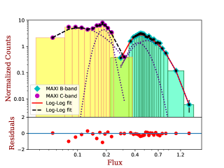
Figure 1: Top Panel : Histograms of the long-term X-ray flux distribution of Cygnus X-1 obtained using the MAXI B-band and C-band archive light curve. The green diamond points correspond to B-band light curves, while violet filled circles correspond to C-band light curve. Histogram with yellow and green colors corresponds to C-band and B-band respectively. The two curves (solid and dashed curves) shown are the best fitted double-log-normal PDF such that red solid curve corresponds to the B-band and black dashed curve corresponds C-band histogram. Dotted curves are the individual log-normal components. Bottom panel : Residuals

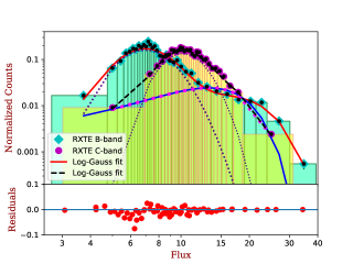
Figure 2: Top panel : Histograms of the long-term X-ray flux distribution of Cygnus X-1 obtained using the RXTE B-band and C-band archive light curve. The green diamond points correspond to B-band histogram, while violet filled circles correspond to C-band light curve. Histogram with yellow and green colors corresponds to C-band and B-band respectively. The two curves (solid and dashed curves) shown are the best fitted log-normal+Gaussian PDF such that red solid curve corresponds to the B-band and black dashed curve corresponds C-band histogram. Dotted curves are the individual log-normal components. Solid(Blue) and dotted(fuchsia) curves are the individual Gaussian components for B and C bands respectively. Bottom panel : Residuals

Table 1: Best fit parameter values of double PDF’s fitted to the flux histograms of MAXI B & C band. Col:- 1: PDF , 2-9: Best fit values of $\mu_{1}$, $\sigma_{1}$, $\mu_{2}$, $\sigma_{2}$, $\mu_{11}$, $\sigma_{11}$, $\mu_{21}$ and $\sigma_{21}$, 10: fraction parameter and 11: Reduced $\chi^{2}$ (degrees of freedom )

MAXI B band C band PDF $\mu_{1}(\times 10^{-1})$ $\sigma_{1}(\times 10^{-1})$ $\mu_{2}(\times 10^{-1})$ $\sigma_{2}(\times 10^{-1})$ $\mu_{11}(\times 10^{-1})$ $\sigma_{11}(\times 10^{-1})$ $\mu_{22}(\times 10^{-1})$ $\sigma_{22}(\times 10^{-1})$ $f_{h}$ $\chi_{\rm red}^{2}$(dof) Log & Log 4.4$\pm$0.13 1.9$\pm$0.12 5.8$\pm$0.05 3.0$\pm$0.12 1.2$\pm$ 0.01 4.8$\pm$0.12 1.9$\pm$0.01 1.4$\pm$0.13 0.29$\pm$0.02 1.06(26) Log & Gauss 4.6$\pm$0.04 1.6$\pm$0.11 6.0$\pm$ 0.08 2.0$\pm$0.06 1.2$\pm$0.01 4.9$\pm$0.14 1.8$\pm$ 0.02 0.2$\pm$0.02 0.34 $\pm$0.02 1.96(26) Gauss & Gauss 4.5$\pm$0.05 0.6$\pm$0.06 6.0$\pm$0.08 1.9$\pm$0.05 0.8$\pm$0.02 0.2$\pm$0.02 1.8$\pm$ 0.03 0.5$\pm$0.01 0.27 $\pm$0.02 3.33(26)

Table 2: Best fit parameter values of double PDF’s fitted to the flux histograms of RXTE B & C band. Col:- 1: PDF , 2-9: Best fit values of $\mu_{1}$, $\sigma_{1}$, $\mu_{2}$, $\sigma_{2}$, $\mu_{11}$, $\sigma_{11}$, $\mu_{21}$ and $\sigma_{21}$, 10: fraction parameter and 11: Reduced $\chi^{2}$ (degrees of freedom )

RXTE B band C band PDF $\mu_{1}$ $\sigma_{1}(\times 10^{-1})$ $\mu_{2}$ $\sigma_{2}$ $\mu_{11}$ $\sigma_{11}(\times 10^{-1})$ $\mu_{22}$ $\sigma_{22}$ $f_{h}$ $\chi_{\rm red}^{2}$(dof) Log & Gauss 6.42 $\pm$0.05 2.6$\pm$0.09 13.32$\pm$0.90 8.00$\pm$0.43 9.48$\pm$0.08 2.1$\pm$0.08 12.17$\pm$0.31 5.45$\pm$ 0.26 0.66 $\pm$0.02 1.20(55) Log & Log 6.48$\pm$0.06 2.9$\pm$0.09 16.94$\pm$0.67 0.31$\pm$0.02 9.87$\pm$ 0.08 2.4$\pm$0.08 11.02$\pm$0.04 0.54$\pm$0.04 0.78$\pm$0.01 1.55(55) Gauss & Gauss 6.42 $\pm$0.07 1.50$\pm$0.07 13.08$\pm$1.22 7.70$\pm$0.63 9.37$\pm$0.12 1.91$\pm$0.11 12.96$\pm$0.56 4.81$\pm$ 0.26 0.62 $\pm$0.03 2.70(55)

4 Comparison with Spectral States

In addition to Hard and Soft spectral states, Cygnus X-1 also exhibits an Intermediate spectral state characterized by a moderately strong thermal component and relatively soft Hard spectrum (Belloni et al., 1996). The Intermediate state mostly appears when the source is about to make a transition from Hard to Soft state, but fails to do and instead stays in a distinct state, where the X-ray spectral properties lies in between Hard state and Soft state (Belloni et al., 1996; Pottschmidt et al., 2003). Grinberg et al. (2013) have provided an easy-to-use prescription in determining the spectral states of Cygnus X-1 using data from RXTE-ASM and MAXI. For convenience, we have repeated the state definitions of Hard, Soft and Intermediate states of Cygnus X-1 in Table 3. Using these definitions, we separated the B-band and C-band data of RXTE-ASM and MAXI into Hard, Soft and Intermediate states. The Table also shows the number of observations per state and the corresponding percentage.

For MAXI data, there is a interesting correspondence between the Hard and Soft states and the flux distribution components obtained in the simultaneous fitting of B and C band histograms with double PDF. The best fit centroid values of the two components matches closely with the average of the fluxes of the Hard and Soft states (see table 4). We note that for MAXI observations, the fraction of time the source is in the Intermediate State is $\sim 4$% and hence including them as being part of either the Hard or Soft state, does not change the flux averages or their fraction of time spent in them. However, the fraction of time spend in the Hard state based on spectral classification ($\sim 39.8$%) deviates from that obtained by flux distribution fitting $f_{h}=29\pm 2$% (see table 1). It should be noted here that in case of MAXI, the criterion $SNR>5$ for each time bin in both the B and C bands removes significant number of timebins (11% of the total data). We found these timebins gets preferentially removed from the hard state. This means that the obtained $f_{h}=29\pm 2\%$ value would be significantly lower than the actual time spend by the source in the hard state. If we consider that the 10% of removed data belongs to the hard state, then $f_{h}$ would turn out to be $\sim 39\%$, which is much close to the value obtained from the spectral classification ($\sim 39.8\%$).

For RXTE data, the best fit centroid value and the average flux value for the hard state matches well with that found by the flux distribution fitting as shown in Table 4., but a deviation can be seen for the second component i.e. with the Soft state. Here, the Intermediate state is represented by a significant fraction of the observations $\sim 11$% comparable to the Soft state. As shown in Table 4, combining the Intermediate and the Soft state observations does not alleviate the discrepancy between the spectral and flux distribution classification. Moreover, we found that the fraction of time spend in the Hard state based on spectral classification ($\sim 77.45$%) also deviates from that obtained by flux distribution fitting $f_{h}=66\pm 2$% (see table 2). However, in case of RXTE, only small fraction of timebins (2.9%) gets removed by SNR criteria, and therefore the discrepancy can not accounted for the timebins removed by SNR criteria.

We consider the possibility that the flux distribution should be represented by three components corresponding to the Hard, Soft and Intermediate spectral states. Thus, we attempted to fit triple combinations of log-normal and Gaussian to the histograms. Since the number of free parameters are large, we constrain the centroids of two of the components to match with the average fluxes of the Soft and Intermdiatory states. As shown in Table 5), for various combinations, the $\chi^{2}_{red}$ is not smaller than what was obtained for the two component fit and hence we infer that there is no evidence for the flux distribution to be represented by three components each being either a log-normal or a Gaussian.

The results of this work can be graphically summarized by multiplots as shown in Figure 3 for RXTE/ASM and Figure 4 for MAXI. The top and right panels are the flux histogram with the best fit two component models. In the central panel, the C-band and B-Band fluxes are plotted against each other and the points corresponding to the Hard, Soft and Intermediate States (as defined by Grinberg et al. (2013)) are shown using different point types (and color). The vertical and horizontal solid bands represent the centroid values of the components used to fit the flux histograms with the widths equal to their errors. Large size points mark the average flux values of the Soft, Hard and Soft+Intermediate states. For both energy bands and for both the instruments, the average of the Hard state coincides with the best fit centroid values. The average of the Soft+Intermediate states are closer to the corresponding centroid values as compared to the Soft state alone.

Table 3: The state definitions of RXTE-ASM data and MAXI described by Grinberg et al., 2013. Col:- 1: States of Cygnus X-1, 2: Criteria for identifying spectral states of Cygnus X-1 using RXTE-ASM observation, 3: Criteria for identifying states of Cygnus X-1 for MAXI observations, 4 & 5: Number of data points, N with their percentage that fall into each of the states using RXTE-ASM and MAXI observation. In Col 2, c is count rate (counts $\rm s^{-1}$) in energy band $\sim$1.5-12 keV, h is hardness ratio defined as ratio of count rates in RXTE C-band ($5-12$ keV) and A-band ($1.5-3$ keV) and $h_{0}$=0.28. In Col 3, $c_{M}$ is count rate in energy range $\sim 2-4$ keV, $h_{M}$ is MAXI hardness defined as $4-10$ keV / $2-4$ keV (B-band/A-band)

State RXTE-ASM MAXI N(Percentage) N(Percentage) using RXTE-ASM using MAXI Hard state c $\leq$ 20 $\vee$ c $\leq$ 55 $\times(h-h_{0})$ $c_{M}$ $\leq$ 1.4$\times(h_{M})$ 3598(77.45%) 763(39.78%) Interm. state c $>$ 20 $\wedge$ 55 $\times(h-h_{0})$ $<$ c $\leq$ 350 $\times(h-h_{0})$ 1.4$\times(h_{M})$ $<$ $c_{M}$ $\leq$ 8/3$\times(h_{M})$ 523(11.25%) 81(4.22%) Soft state c $>$ 20 $\wedge$ c $>$ 350 $\times(h-h_{0})$ 8/3$\times(h_{M})$ $<$ c 524(11.28%) 1074(55.99%)

Table 4: Centroid values obtained from Double PDF’s fitting and Mean values of different spectral states of B and C bands of RXTE and MAXI.

Centroid Values of PDF Mean of Spectral State Energy band $\mu_{H}$ $\mu_{S}$ mean(H) mean(S) mean(I) mean(H+I) mean(S+I) RXTE B-band 6.42$\pm$0.05 13.32$\pm$0.90 6.49$\pm$0.01 20.08$\pm$0.01 14.01$\pm$0.01 7.15$\pm$0.01 16.78$\pm$0.01 RXTE C-band 9.48$\pm$0.08 12.17$\pm$0.31 9.23$\pm$0.01 12.66$\pm$0.01 14.62$\pm$0.01 9.78$\pm$0.01 13.60$\pm$0.01 MAXI B-band 0.44$\pm$0.02 0.58$\pm$0.005 0.43$\pm$0.01 0.61$\pm$0.01 0.62$\pm$0.01 0.45$\pm$0.01 0.61$\pm$0.01 MAXI C-band 0.19$\pm$0.01 0.12$\pm$0.001 0.18$\pm$0.03 0.11$\pm$0.04 0.19$\pm$0.13 0.18$\pm$0.03 0.11$\pm$0.04

Table 5: Best fit parameter values of the triple PDF’s fitted to the flux histograms of RXTE and MAXI B & C bands. Col:-1: Combination of functions , 2-9: Best fit values of $\mu_{1}$, $\sigma_{1}$, $\sigma_{2}$, $\sigma_{3}$ , $\mu_{11}$ , $\sigma_{11}$ , $\sigma_{22}$ & $\sigma_{33}$, 10-11: Normalization fractions $f_{n1}$ & $f_{n2}$ and 12: $\chi_{\rm red}^{2}$(Degrees of freedom )

RXTE B band C band Norm. Fraction Red. $\chi^{2}$ PDF $\mu_{1}$ $\sigma_{1}(\times 10^{-1})$ $\sigma_{2}$ $\sigma_{3}$ $\mu_{11}$ $\sigma_{11}(\times 10^{-1})$ $\sigma_{22}$ $\sigma_{33}(\times 10^{-1})$ $f_{n1}$ $f_{n2}$ $\chi_{\rm red}^{2}$(dof) Log & Gauss & Gauss 6.48$\pm$0.06 2.9$\pm$0.08 4.22$\pm$1.22 6.17$\pm$0.45 9.39$\pm$0.09 0.21$\pm$0.09 2.27$\pm$ 0.40 6.87 $\pm$0.89 0.77 $\pm$0.01 0.1$\pm$0.03 1.69(55) Log & log & log 6.48$\pm$0.06 2.9$\pm$0.07 0.30$\pm$0.05 0.25$\pm$0.01 9.48$\pm$0.09 2.2$\pm$0.08 0.17$\pm$ 0.03 0.92 $\pm$0.24 0.77 $\pm$0.01 0.1$\pm$0.02 1.34(55) MAXI Log & log & log 0.44$\pm$0.01 0.21$\pm$0.01 0.23$\pm$0.11 0.27$\pm$0.01 1.0$\pm$0.05 0.35$\pm$0.03 0.12$\pm$0.05 0.20 $\pm$0.01 0.45 $\pm$0.05 0.09$\pm$0.05 1.17(25) Log & gauss & gauss 0.45$\pm$0.01 0.17$\pm$0.02 0.13$\pm$0.01 0.24$\pm$0.02 1.0$\pm$0.04 0.36$\pm$0.03 0.08$\pm$0.01 0.02 $\pm$0.03 0.34 $\pm$0.06 0.35$\pm$0.11 1.37(25)

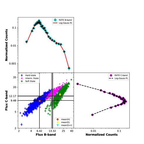
Figure 3: Multiplot of Cygnus X-1 obtained using the RXTE-ASM observations. The top and bottom-right panels are the histograms of long-term X-ray flux distributions of B and C band archive light curves. The curves (red and black-dashed curves) are the best fitted double PDF (log-normal+Gaussian). Bottom-left panel is the plot between the B-band and C-band flux’s with the Hard, Inter-mediate and Soft states highlighted by colors blue, orange and green respectively. The vertical and horizontal gray bands indicate the centroids of log-normal+Gaussian PDF fit to the histograms of B and C bands with widths representing 1-$\sigma$ error range. Large size points with colors red, cyan and yellow mark the mean flux points of Hard, Soft+Intermediate and Soft states respectively.

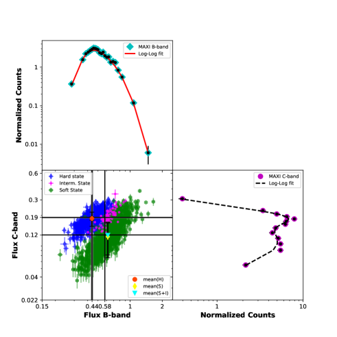
Figure 4: Multiplot of Cygnus X-1 obtained using the MAXI observations. The top and bottom-right panels are the histograms of long-term X-ray flux distributions of B and C band archive light curves. The curves (red and black-dashed curves) are the best fitted double log-normal PDF’. Bottom-left panel is the plot between the B-band and C-band flux’s with the Hard, Inter-mediate and Soft states highlighted by colors blue, orange and green respectively. The vertical and horizontal gray bands indicate the centroids of double-log-normal PDF fit to the histograms of B and C bands respectively with widths representing 1-$\sigma$ error range. Large size points with colors red, cyan and yellow represent the mean flux points of Hard, Soft+Intermediate and Soft states respectively.

5 Summary and Discussion

We have analyzed the long term flux distribution of Cygnus X-1 using RXTE/ASM and MAXI data in two energy bands. We fit the distributions using two components which we consider to be either a log-normal or a Gaussian one. For MAXI data, both the components are better represented by a log-normal distribution, rather than a Gaussian one, and they can be clearly identified with the Hard and Soft spectral states. The centroid values of the two components and the fraction of time they occur are consistent with the independent spectral-timing classification undertaken by Grinberg et al. (2013). Thus, this implies that the long term flux distribution of Cygnus X-1 is the same as for its short term one. From time-scales of seconds to week, the variability of the source seems to be determined by an multiplicative process leading to log-normal distributions. It is attractive to associate a single process such as a stochastic propagation model where perturbations in different time-scales originating at different radii of the disk have a multiplicative effect on the inner accretion rate leading to X-ray variability (Lyubarskii, 1997). However, there are other possibilities such as Gaussian variability of spectral index (Sinha et al., 2018) and emission from large number of randomly oriented mini-jets (Biteau and Giebels, 2012) which can give rise to a log-normal flux distribution and it is not certain whether these different mechanisms are active on different time-scales.

For RXTE/ASM data, one of the components is better described as a log-normal one and its centroid value and fraction of occurrence time is close to that obtained from spectral classification of Grinberg et al. (2013) for the Hard state. For MAXI data, each of the components is better fitted by a log-normal distribution. Their best fit centroids and fraction of time the source spends being in that component are consistent with those of the Hard and Soft spectral states. Thus, the MAXI result, that the Hard state’s long term distribution is a log-normal one, is corroborated by the RXTE data. However, for the second distribution the results are in contradiction since the best fit obtained is a Gaussian function instead of a log-normal one. Further, the centroid of the component does not match well with the average flux of the Soft state nor of the Soft and Intermediate states together.

If we consider the Intermediate state as a distinct state as defined by Grinberg et al. (2013) than one obvious reason for the discrepancy between the MAXI and the RXTE/ASM results might be the presence of observations classified as Intermediate state. For MAXI data such observations only account for $\sim 4$% of the total data while for RXTE/ASM it is significantly larger at $\sim 11.25\%$ and comparable to the Soft State fraction of $\sim 11.28$%. To check whether observations showing Intermediate spectral and temporal behavior belong to a separate state or not, we attempted to fit the long term flux histograms with three components. Since the number of parameters for a three component fit (thirteen) was too many given the data set, we took guidance from the spectral classification by Grinberg et al. (2013) to fix the centroid fluxes for the soft and Intermediate components to the mean values of these classes. The reduced $\chi^{2}$ obtained were larger than those obtained for a two component fit for both ASM and MAXI data. Thus, we were not able to find any indications for the presence of three flux distribution components. It should be noted that if the Intermediate state observations correspond to times when the source is making a transition between the Soft and Hard states (i.e. it is not a distinct state by itself) then their flux distribution may not correspond to a Gaussian (or log-normal) and instead could be some arbitrary function. In that case, flux distribution fitting may not reveal their nature since such complex triple component fits may always be degenerate.

The two spectral components that dominate the Soft state spectra (i.e. a thermal disk emission and a power-law Comptonization one) may have different distributions. We tried to check this by fitting the soft state flux distributions by a Gaussian for the MAXI B band and by a log-normal for the MAXI C band and vice-versa However, the reduced $\chi^{2}$ for a double log-normal description was found to be smaller that such combinations. Since the C-band may be dominated by the power-law emission and the B-Band by the thermal one, this implies that both the thermal disk emission and the power-law one follow log-normal distributions.

Analysis of a large number of pointed observations by a more sensitive instrument like the RXTE/PCA will provide significantly better information than the sky monitor data used here. Moreover, such an analysis can be undertaken for finer energy bins to quantify differences, if any, between the flux distributions of different spectral components. However, for such an analysis, the serious bias introduced by uneven sampling and by observations preferentially undertaken when the source was in an unusual state has to be addressed.

The flux distribution analysis shows that fraction of time Cygnus X-1 was in a Hard state during the RXTE era, $\sim 0.7$, was significantly higher than during the MAXI observations, $\sim 0.3$. This implies behavioral changes on time-scales of decades. The change in spectral state of Cygnus X-1 in recent years has been reported in earlier studies as well (Grinberg et al., 2013; Sugimoto et al., 2016). It is interesting to note that there are black hole systems (such as LMC X-1) which are always observed to be in the Soft state and it maybe possible that after many decades, a system like Cygnus X-1 may evolve, such that it also spends most of its time in one particular state. We emphasis that classification based on spectral and timing properties of a source provide valuable insight into the nature of the system and in particular are extremely useful in making predictions for the source behavior. On the other hand, flux distribution analysis reveal the number of distinct dynamic configurations (i.e. broadly corresponding to different flux levels) a system can be in. If the two analysis are consistent as seen for the MAXI data, then it reinforces the distinct spectral/timing properties of a system for a given configuration. These configurations may correspond to hydro-dynamical steady state solutions of accreting systems which co-exist for a given determining parameter such as the accretion rate or the system may make transition from one solution to another when the parameter changes (Shapiro et al., 1976; Narayan and Yi, 1994).

Unlike Cygnus X-1 which is persistent, many black hole systems exhibit outburst which last for several months and which occur on once in several years. They show a wide range of flux levels with different spectral and timing properties. A flux distribution analysis will require observations of a significant number of outbursts, otherwise the analysis will be biased by a few dominant ones. On the other hand, flux distribution studies can be undertaken on persistent sources (including Neutron star systems) using monitoring instruments with repeated and unbiased pointed observations.

6 ACKNOWLEDEMENTS

K. Deka would like to thank University Grants Commission of India and Tezpur University for all the support. K. Deka acknowledges the support of IUCAA under the visitor’s program, most part of this research work is carried under this program. G.A. Ahmed would like to thank IUCAA for associateship. This research work has made use of MAXI data provided by RIKEN, JAXA, and the MAXI team, and RXTE-ASM light curves provided by the ASM/RXTE team.

References

- Bałucińska-Church et al. (2000) Bałucińska-Church, M., Church, M.J., Charles, P.A., Nagase, F., LaSala, J., Barnard, R., 2000. The distribution of X-ray dips with orbital phase in Cygnus X-1. mnras 311, 861–868. doi:10.1046/j.1365-8711.2000.03149.x, arXiv:astro-ph/9909235.
- Belloni et al. (1996) Belloni, T., Mendez, M., van der Klis, M., Hasinger, G., Lewin, W.H.G., van Paradijs, J., 1996. An Intermediate State of Cygnus X-1. apjl 472, L107. doi:10.1086/310369.
- Biteau and Giebels (2012) Biteau, J., Giebels, B., 2012. The minijets-in-a-jet statistical model and the rms-flux correlation. aap 548, A123. doi:10.1051/0004-6361/201220056, arXiv:1210.2045.
- Boroson and Vrtilek (2010) Boroson, B., Vrtilek, S.D., 2010. X-ray Variations at the Orbital Period from Cygnus X-1 IN the High/Soft State. apj 710, 197–206. doi:10.1088/0004-637X/710/1/197, arXiv:0912.5412.
- Bowyer et al. (1965) Bowyer, S., Byram, E.T., Chubb, T.A., Friedman, H., 1965. Cosmic X-ray Sources. Science 147, 394–398. doi:10.1126/science.147.3656.394.
- Brocksopp et al. (1999) Brocksopp, C., Fender, R.P., Larionov, V., Lyuty, V.M., Tarasov, A.E., Pooley, G.G., Paciesas, W.S., Roche, P., 1999. Orbital, precessional and flaring variability of cygnus x-1. Monthly Notices of the Royal Astronomical Society 309, 1063–1073. URL: http://dx.doi.org/10.1046/j.1365-8711.1999.02919.x, doi:10.1046/j.1365-8711.1999.02919.x.
- Frontera et al. (1975) Frontera, F., Fuligni, F., Cavani, C., 1975. Long term variability of CYG X-1 in hard X-rays. apss 32, 197–203. doi:10.1007/BF00646225.
- Gaskell (2004) Gaskell, C.M., 2004. Lognormal X-Ray Flux Variations in an Extreme Narrow-Line Seyfert 1 Galaxy. apjl 612, L21–L24. doi:10.1086/424565.
- Gies and Bolton (1986) Gies, D.R., Bolton, C.T., 1986. The optical spectrum of HDE 226868 = Cygnus X-1. II Spectrophotometry and mass estimates. apj 304, 371–393. doi:10.1086/164171.
- Gies et al. (2003) Gies, D.R., Bolton, C.T., Thomson, J.R., Huang, W., McSwain, M.V., Riddle, R.L., Wang, Z., Wiita, P.J., Wingert, D.W., Csák, B., Kiss, L.L., 2003. Wind Accretion and State Transitions in Cygnus X-1. apj 583, 424–436. doi:10.1086/345345, arXiv:astro-ph/0206253.
- Gleissner et al. (2004) Gleissner, T., Wilms, J., Pottschmidt, K., Uttley, P., Nowak, M.A., Staubert, R., 2004. Long term variability of Cyg X-1. II. The rms-flux relation. aap 414, 1091–1104. doi:10.1051/0004-6361:20031684, arXiv:astro-ph/0311039.
- Grinberg et al. (2013) Grinberg, V., Hell, N., Pottschmidt, K., Böck, M., Nowak, M.A., Rodriguez, J., Bodaghee, A., Cadolle Bel, M., Case, G.L., Hanke, M., Kühnel, M., Markoff, S.B., Pooley, G.G., Rothschild, R.E., Tomsick, J.A., Wilson-Hodge, C.A., Wilms, J., 2013. Long term variability of Cygnus X-1. V. State definitions with all sky monitors. aap 554, A88. doi:10.1051/0004-6361/201321128, arXiv:1303.1198.
- Grinberg et al. (2015) Grinberg, V., Leutenegger, M.A., Hell, N., Pottschmidt, K., Böck, M., García, J.A., Hanke, M., Nowak, M.A., Sundqvist, J.O., Townsend, R.H.D., Wilms, J., 2015. Long term variability of Cygnus X-1. VII. Orbital variability of the focussed wind in Cyg X-1/HDE 226868 system. aap 576, A117. doi:10.1051/0004-6361/201425418, arXiv:1502.07343.
- Heil and Vaughan (2010) Heil, L.M., Vaughan, S., 2010. The linear rms-flux relation in an ultraluminous x-ray source. Monthly Notices of the Royal Astronomical Society: Letters 405, L86–L89. URL: http://dx.doi.org/10.1111/j.1745-3933.2010.00864.x, doi:10.1111/j.1745-3933.2010.00864.x.
- Heil et al. (2011) Heil, L.M., Vaughan, S., Uttley, P., 2011. Quasi-periodic oscillations in XTE J1550-564: the rms-flux relation. mnras 411, L66–L70. doi:10.1111/j.1745-3933.2010.00997.x, arXiv:1011.6321.
- Herrero et al. (1995) Herrero, A., Kudritzki, R.P., Gabler, R., Vilchez, J.M., Gabler, A., 1995. Fundamental parameters of galactic luminous OB stars. II. A spectroscopic analysis of HDE 226868 and the mass of Cygnus X-1. aap 297, 556.
- Lachowicz et al. (2006) Lachowicz, P., Zdziarski, A.A., Schwarzenberg-Czerny, A., Pooley, G.G., Kitamoto, S., 2006. Periodic long-term X-ray and radio variability of Cygnus X-1. mnras 368, 1025–1039. doi:10.1111/j.1365-2966.2006.10219.x, arXiv:astro-ph/0508306.
- Levine et al. (1996) Levine, A.M., Bradt, H., Cui, W., Jernigan, J.G., Morgan, E.H., Remillard, R., Shirey, R.E., Smith, D.A., 1996. First Results from the All-Sky Monitor on the Rossi X-Ray Timing Explorer. apjl 469, L33. doi:10.1086/310260, arXiv:astro-ph/9608109.
- Liang and Nolan (1984) Liang, E.P., Nolan, P.L., 1984. Cygnus X-1 revisited. ssr 38, 353–384. doi:10.1007/BF00176834.
- Lyubarskii (1997) Lyubarskii, Y.E., 1997. Flicker noise in accretion discs. mnras 292, 679. doi:10.1093/mnras/292.3.679.
- Matsuoka et al. (2009) Matsuoka, M., Kawasaki, K., Ueno, S., Tomida, H., Kohama, M., Suzuki, M., Adachi, Y., Ishikawa, M., Mihara, T., Sugizaki, M., Isobe, N., Nakagawa, Y., Tsunemi, H., Miyata, E., Kawai, N., Kataoka, J., Morii, M., Yoshida, A., Negoro, H., Nakajima, M., Ueda, Y., Chujo, H., Yamaoka, K., Yamazaki, O., Nakahira, S., You, T., Ishiwata, R., Miyoshi, S., Eguchi, S., Hiroi, K., Katayama, H., Ebisawa, K., 2009. The MAXI Mission on the ISS: Science and Instruments for Monitoring All-Sky X-Ray Images. pasj 61, 999. doi:10.1093/pasj/61.5.999, arXiv:0906.0631.
- McHardy (1988) McHardy, I., 1988. EXOSAT observations of variability in active galactic nuclei. memsai 59, 239–259.
- Mihara et al. (2011) Mihara, T., Nakajima, M., Sugizaki, M., Serino, M., Matsuoka, M., Kohama, M., Kawasaki, K., Tomida, H., Ueno, S., Kawai, N., Kataoka, J., Morii, M., Yoshida, A., Yamaoka, K., Nakahira, S., Negoro, H., Isobe, N., Yamauchi, M., Sakurai, I., 2011. Gas Slit Camera (GSC) onboard MAXI on ISS. pasj 63, S623–S634. doi:10.1093/pasj/63.sp3.S623, arXiv:1103.4224.
- Miller-Jones et al. (2021) Miller-Jones, J.C.A., Bahramian, A., Orosz, J.A., Mandel, I., Gou, L., Maccarone, T.J., Neijssel, C.J., Zhao, X., Ziółkowski, J., Reid, M.J., Uttley, P., Zheng, X., Byun, D.Y., Dodson, R., Grinberg, V., Jung, T., Kim, J.S., Marcote, B., Markoff, S., Rioja, M.J., Rushton, A.P., Russell, D.M., Sivakoff, G.R., Tetarenko, A.J., Tudose, V., Wilms, J., 2021. Cygnus x-1 contains a 21–solar mass black hole—implications for massive star winds. Science 371, 1046–1049. URL: https://science.sciencemag.org/content/371/6533/1046, doi:10.1126/science.abb3363, arXiv:https://science.sciencemag.org/content/371/6533/1046.full.pdf.
- Narayan and Yi (1994) Narayan, R., Yi, I., 1994. Advection-dominated Accretion: A Self-similar Solution. apjl 428, L13. doi:10.1086/187381, arXiv:astro-ph/9403052.
- Negoro and Mineshige (2002) Negoro, H., Mineshige, S., 2002. Log-Normal Distributions in Cygnus X-1: Possible Physical Link with Gamma-Ray Bursts and Blazars. pasj 54, L69–L72. doi:10.1093/pasj/54.5.L69, arXiv:astro-ph/0208311.
- Orosz et al. (2011) Orosz, J.A., McClintock, J.E., Aufdenberg, J.P., Remillard, R.A., Reid, M.J., Narayan, R., Gou, L., 2011. The Mass of the Black Hole in Cygnus X-1. apj 742, 84. doi:10.1088/0004-637X/742/2/84, arXiv:1106.3689.
- Pottschmidt et al. (2003) Pottschmidt, K., Wilms, J., Nowak, M.A., Pooley, G.G., Gleissner, T., Heindl, W.A., Smith, D.M., Remillard, R., Staubert, R., 2003. Long term variability of Cygnus X-1. I. X-ray spectral-temporal correlations in the hard state. aap 407, 1039–1058. doi:10.1051/0004-6361:20030906, arXiv:astro-ph/0202258.
- Poutanen et al. (2008) Poutanen, J., Zdziarski, A.A., Ibragimov, A., 2008. Superorbital variability of X-ray and radio emission of Cyg X-1 - II. Dependence of the orbital modulation and spectral hardness on the superorbital phase. mnras 389, 1427–1438. doi:10.1111/j.1365-2966.2008.13666.x, arXiv:0802.1391.
- Shapiro et al. (1976) Shapiro, S.L., Lightman, A.P., Eardley, D.M., 1976. A two-temperature accretion disk model for Cygnus X-1: structure and spectrum. apj 204, 187–199. doi:10.1086/154162.
- Sinha et al. (2018) Sinha, A., Khatoon, R., Misra, R., Sahayanathan, S., Mandal, S., Gogoi, R., Bhatt, N., 2018. The flux distribution of individual blazars as a key to understand the dynamics of particle acceleration. mnras 480, L116–L120. doi:10.1093/mnrasl/sly136, arXiv:1807.09073.
- Sugimoto et al. (2017) Sugimoto, J., Kitamoto, S., Mihara, T., Matsuoka, M., 2017. Orbital modulations of X-ray light curves of Cygnus X-1 in its low/hard and high/soft states. pasj 69, 52. doi:10.1093/pasj/psx028, arXiv:1705.04781.
- Sugimoto et al. (2016) Sugimoto, J., Mihara, T., Kitamoto, S., Matsuoka, M., Sugizaki, M., Negoro, H., Nakahira, S., Makishima, K., 2016. MAXI observations of long-term variations of Cygnus X-1 in the low/hard and the high/soft states. pasj 68, S17. doi:10.1093/pasj/psw004, arXiv:1601.02740.
- Sugizaki et al. (2011) Sugizaki, M., Mihara, T., Serino, M., Yamamoto, T., Matsuoka, M., Kohama, M., Tomida, H., Ueno, S., Kawai, N., Morii, M., Sugimori, K., Nakahira, S., Yamaoka, K., Yoshida, A., Nakajima, M., Negoro, H., Eguchi, S., Isobe, N., Ueda, Y., Tsunemi, H., 2011. In-Orbit Performance of MAXI Gas Slit Camera (GSC) on ISS. pasj 63, S635–S644. doi:10.1093/pasj/63.sp3.S635, arXiv:1102.0891.
- Tomida et al. (2011) Tomida, H., Tsunemi, H., Kimura, M., Kitayama, H., Matsuoka, M., Ueno, S., Kawasaki, K., Katayama, H., Miyaguchi, K., Maeda, K., Daikyuji, A., Isobe, N., 2011. Solid-State Slit Camera (SSC) Aboard MAXI. pasj 63, 397–405. doi:10.1093/pasj/63.2.397, arXiv:1101.3651.
- Uttley (2004) Uttley, P., 2004. SAX J1808.4-3658 and the origin of X-ray variability in X-ray binaries and active galactic nuclei. mnras 347, L61–L65. doi:10.1111/j.1365-2966.2004.07434.x, arXiv:astro-ph/0311453.
- Uttley and McHardy (2001) Uttley, P., McHardy, I.M., 2001. The flux-dependent amplitude of broadband noise variability in X-ray binaries and active galaxies. Monthly Notices of the Royal Astronomical Society 323, L26–L30. URL: https://doi.org/10.1046/j.1365-8711.2001.04496.x, doi:10.1046/j.1365-8711.2001.04496.x, arXiv:https://academic.oup.com/mnras/article-pdf/323/2/L26/4079417/323-2-L26.pdf.
- Uttley et al. (2005) Uttley, P., McHardy, I.M., Vaughan, S., 2005. Non-linear X-ray variability in X-ray binaries and active galaxies. mnras 359, 345–362. doi:10.1111/j.1365-2966.2005.08886.x, arXiv:astro-ph/0502112.
- Vaughan et al. (2003) Vaughan, S., Edelson, R., Warwick, R.S., Uttley, P., 2003. On characterizing the variability properties of X-ray light curves from active galaxies. mnras 345, 1271–1284. doi:10.1046/j.1365-2966.2003.07042.x, arXiv:astro-ph/0307420.
- Vrtilek and Boroson (2013) Vrtilek, S.D., Boroson, B.S., 2013. Model independent means of categorizing X-ray binaries - I. Colour-colour-intensity diagrams. mnras 428, 3693–3714. doi:10.1093/mnras/sts312.
- Wen et al. (1999) Wen, L., Cui, W., Levine, A.M., Bradt, H.V., 1999. Orbital Modulation of X-Rays from Cygnus X-1 in its Hard and Soft States. apj 525, 968–977. doi:10.1086/307917.
- Wilms et al. (2006) Wilms, J., Nowak, M.A., Pottschmidt, K., Pooley, G.G., Fritz, S., 2006. Long term variability of Cygnus X-1. IV. Spectral evolution 1999-2004. aap 447, 245–261. doi:10.1051/0004-6361:20053938, arXiv:astro-ph/0510193.
- Zdziarski et al. (2002) Zdziarski, A.A., Poutanen, J., Paciesas, W.S., Wen, L., 2002. Understanding the Long-Term Spectral Variability of Cygnus X-1 with Burst and Transient Source Experiment and All-Sky Monitor Observations. apj 578, 357–373. doi:10.1086/342402, arXiv:astro-ph/0204135.