First results of the CAST-RADES haloscope search for axions at 34.67 $\boldsymbol{\mu}$eV

Abstract

We present results of the Relic Axion Dark-Matter Exploratory Setup (RADES), a detector which is part of the CERN Axion Solar Telescope (CAST), searching for axion dark matter in the 34.67 $\mu$eV mass range. A radio frequency cavity consisting of 5 sub-cavities coupled by inductive irises took physics data inside the CAST dipole magnet for the first time using this filter-like haloscope geometry. An exclusion limit with a 95% credibility level on the axion-photon coupling constant of g${}_{a\gamma}\gtrsim 4\times 10^{-13}\,\mathrm{GeV^{-1}}$ over a mass range of $34.6738\,\mathrm{\mu eV}<m_{a}<34.6771\,\mathrm{\mu eV}$ is set. This constitutes a significant improvement over the current strongest limit set by CAST at this mass and is at the same time one of the most sensitive direct searches for an axion dark matter candidate above the mass of 25 $\mu$eV. The results also demonstrate the feasibility of exploring a wider mass range around the value probed by CAST-RADES in this work using similar coherent resonant cavities.

1 Introduction

Astrophysical observations and the standard $\Lambda$ Cold Dark Matter model of the big bang cosmology indicate that around $\sim 84\,\mathrm{\%}$ of the matter in the Universe is dark matter Ade:2015xua ; Bertone:2004pz ; Clowe:2006eq . A suitable candidate for dark matter is the quantum chromodynamics (QCD) axion Weinberg:1977ma ; Wilczek:1977pj . This pseudoscalar particle was first introduced to solve the strong Charge Conjugation-Parity (CP) problem via the Peccei-Quinn mechanism Peccei:1977hh ; Peccei:1977ur . Later on it was realized that the axion has the right properties and the proper production mechanism to be a cold dark matter candidate Abbott:1982af ; Dine:1982ah . Depending on when the Peccei-Quinn symmetry is broken, the production of axions in the early universe can happen before Tanabashi:2018oca or after inflation. The post-inflationary scenario predicts axion dark matter masses above roughly 25 $\mu$eV Kawasaki:2014sqa ; Fleury:2015aca . Benchmark QCD axions follow a strict mass-photon coupling relation. However, variant models allow QCD axions with enhanced coupling to photons Agrawal:2017cmd ; DiLuzio:2016sbl , and generic axion-like particles (not related to the solution of the strong CP problem) may constitute dark matter with larger couplings than a benchmark axion Arias:2012az . A recent review of axion cosmology and the search for axions is given in Irastorza:2018dyq .

One way of detecting this particle is by the process in which the axion is converted into a photon in the presence of a strong static magnetic field, the inverse Primakoff effect Pirmakoff:1951pj ; Sikivie:1983ip . The axion signal power is enhanced using a resonant cavity with a resonance frequency corresponding to the axion mass tested ($\nu=m_{a}c^{2}/h$). This is known as the haloscope detection method and was first introduced by Pierre Sikivie in 1983 Sikivie:1983ip . The expected power extracted from the cavity due to the axion-photon coupling is given by the following equation Sikivie:1983ip ; Krauss:1985ub ; Kenany:2016tta :

$$P_{a}=g_{a\gamma}^{2}\rho_{\text{DM}}\frac{\beta}{1+\beta}\frac{1}{m_{a}}B^{2}VQ_{L}G^{2},$$ (1)

where $g_{a\gamma}$ is the axion coupling to two photons, $\rho_{\text{DM}}=0.45\,\mathrm{GeVcm^{-3}}$ Read:2014qva is the local dark matter density, $m_{a}$ is the axion mass, $B$ is the magnetic field strength, $V$ is the volume of the cavity, $Q_{L}$ is its loaded quality factor, $G$ is a geometric factor that basically represents the overlap of the cavity resonant mode with the magnetic field and $\beta$ is the coupling between the cavity and the receiver chain.

The axion signal generated in the cavity would appear as an increment over the background thermal noise. For this increment to be measurable, the fluctuations of the power measurement must be sufficiently small, which requires long integration times. The noise power in the cavity is given by:

$$P_{N}=k_{b}T_{\text{sys}}\Delta\nu,$$ (2)

where $k_{b}$ is the Boltzmann constant, $T_{\text{sys}}$ is the system noise temperature and $\Delta\nu$ is the resolution bandwidth of our data acquisition system (DAQ). For the scenario where $\Delta\nu=\Delta\nu_{a}$, Dicke’s radiometer equation can be used to set a target signal-to-noise ratio (SNR) Dicke:1946glx :

$$\text{SNR}=\frac{P_{a}\sqrt{t\Delta\nu_{a}}}{P_{N}},$$ (3)

where $t$ is the total integration time, $\Delta\nu_{a}$ is the axion bandwidth and $P_{a}$ is the axion power.

Many experiments , see e.g.Du:2018uak ; Braine:2019fqb ; Zhong:2018rsr ; Lee:2020cfj , have successfully implemented the haloscope technique to set limits to the axion coupling at low mass ranges (mainly below 25 $\mu$eV). Most of the haloscope detectors use a cylindrical cavity in a solenoidal magnet. In order for these detectors to resonate at higher frequency and search for higher axion masses, naively the radius of the cylinder has to be reduced. This, in turn, decreases the total volume of the detector which reduces its sensitivity to the axion signal (see equation (1)). A way to overcome this issue is to create substructures in the cavity to make the cavity resonate at a higher frequency without losing in volume. This is the concept behind our work. A similar idea led to the development of multiple cell cylindrical cavities Jeong:2017hqs ; Jeong:2020cwz .

This work is based on the idea of using dipole magnets to search for axions using haloscopes Baker:2011na . The Relic Axion Dark-Matter Exploratory Setup (RADES), a detector which is installed in the CERN Axion Solar Telescope (CAST)Anastassopoulos:2017ftl , uses a new type of cavity geometry where a long rectangular cavity is divided into smaller sub-cavities Melcon:2018dba to search for axion masses above 30 $\mu$eV. These cavities can resonate at higher frequencies (between 8 and 9 GHz) and can be coupled together to increase the volume. This technology can thus, in principle, take advantage of the large volume offered by dipole magnets in order to increase the sensitivity to the axion. Other groups are developing complementary techniques TheMADMAXWorkingGroup:2016hpc ; BRASS or performed searches at higher masses using new cavity geometries Alesini:2019ajt ; Alesini:2020vny ; McAllister:2017lkb ; Backes:2020ajv , but at 34.67 $\mu$eV the best limit so far was placed by CAST’s solar axion searches Anastassopoulos:2017ftl .

In 2018 the first CAST-RADES prototype was installed inside one of the CAST’s magnet bores. In this work the results of the 2018 acquisition campaign are presented. Section 2 briefly outlines the chosen cavity design, its properties and details the experimental setup and the characterization of the quantities involved in equation (1). Section 3 gives an overview of the analysis procedure and presents the results of the measurements. In section 4 the results are discussed and prospects for the future are summarized.

2 Experimental Setup

The CAST-RADES detector used in this work consists of a 316LN stainless steel cavity, coated with a $30\,\mathrm{\mu m}$ thick copper layer. The cavity is internally divided in 5 sub-cavities interconnected by inductive irises, resembling a filter-like structure. A complete description of the cavity can be found in reference Melcon:2018dba , here we briefly revisit the main characteristics. The left panel of figure 1 shows a picture of the cavity before and after copper coating. The right panel of figure 1 shows the electric field pattern of the different resonant modes. The axion couples to the first mode at an axion mass of $34.67\,\mathrm{\mu eV}$, which corresponds to a frequency of 8.384 GHz. This frequency corresponds to the wave-guide dimensions that fit into the CAST cold bore Melcon:2018dba . The volume and geometric factor were calculated using the CST simulation software CST .

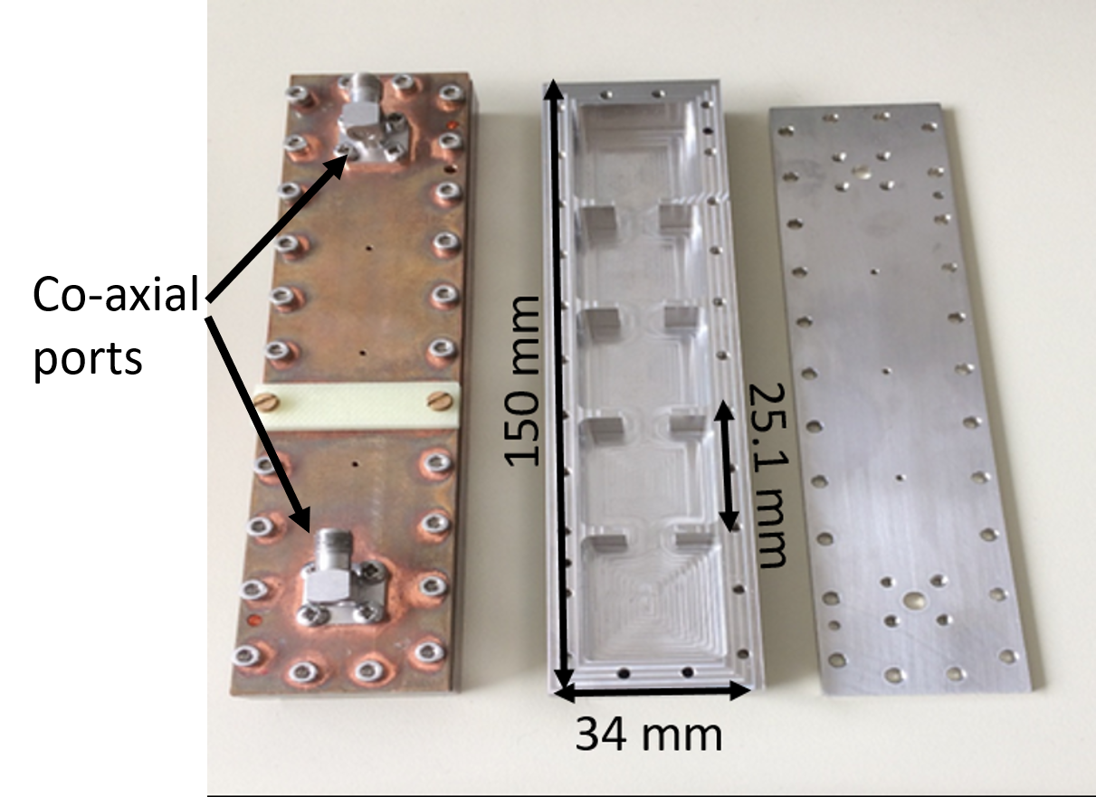
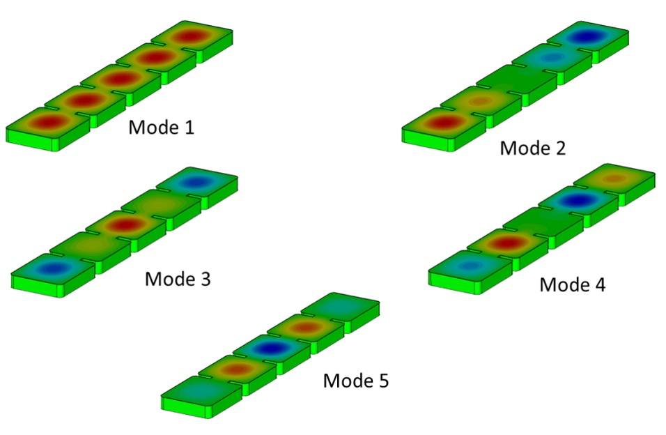
Figure 1: Left: CAST-RADES cavity after copper coating (closed) and before the copper coating (opened). Right: Electric field pattern of the cavity modes Melcon:2018dba , where red and blue indicate opposite directions of the electric field. The first mode, in which the electric field in all sub-cavities is parallel to the external magnetic field, couples to the axion.

The cavity has two 50 $\Omega$ subminiature version A coaxial ports located at each of the extremities, see left panel of figure 1. One port ($P_{1}$) is used to extract the signal during the data-taking period, and must be critically coupled to the cavity to maximize the sensitivity. The second port ($P_{2}$) is used to inject a known input signal to characterize the cavity (e.g. noise temperature or the frequencies of the cavity resonance modes). It is very weakly coupled to avoid signal leakage and reduce the noise coming into the cavity from this port. The cavity is placed inside the CAST dipole magnet. Figure 2 shows a schematic of the CAST-RADES setup. When the magnet is energized, the magnetic field strength at the position of the cavity is 8.8 T. The environmental temperature is (1.8 $\pm$ 0.1) K. Measurements of the cavity response at cryogenic temperatures but in the absence of a magnetic field have been performed and have served as reference data called magnet-off data ($\mathcal{B}_{\rm off}$).

Port $P_{1}$ is connected with coaxial cables to a 40 decibels (dB) TXA4000 cryogenic low noise amplifier (LNA) manufactured by TTI Norte located in a copper vessel at the end cap of the CAST magnet, in a region with negligible magnetic field ($B\ll 0.01\,\mathrm{T}$), but still at cryogenic temperatures. Both $P_{2}$ and $P_{2}$ are connected with semi-rigid coaxial cables to the outside of the cryostat through feedthroughs, as shown in the schematics of Figure 2. The line 1 is then connected to our data acquisition system (DAQ).

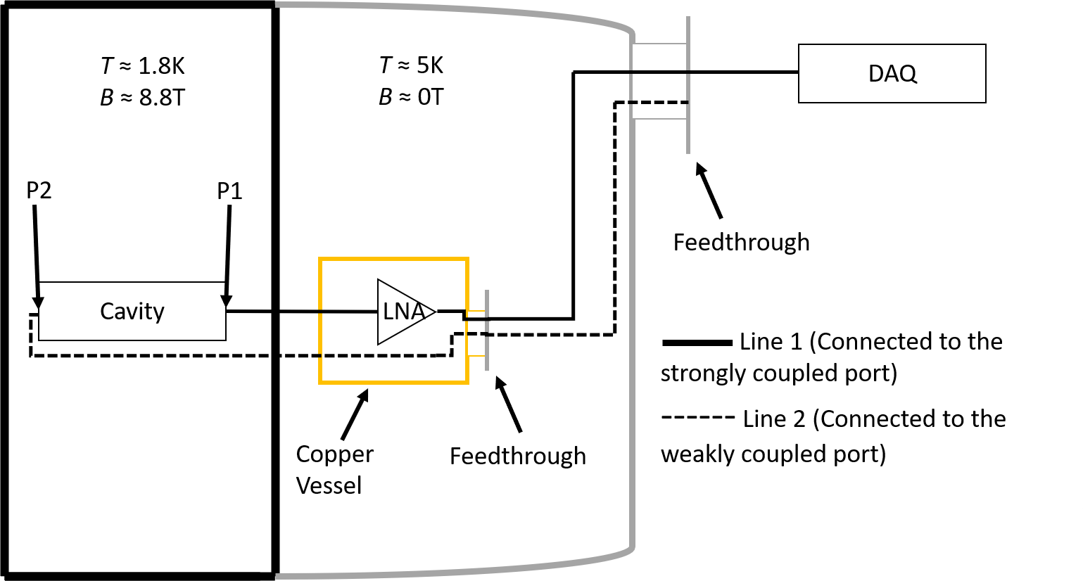
Figure 2: Schematics of the CAST-RADES setup. The cavity is located inside one of the bores of the CAST magnet in a region with $B\approx$ 8.8 T at $T\approx$ 1.8 K. The critically-coupled port ($P_{1}$) is connected through a coaxial cable to the LNA, which is located in a region with negligible magnetic field ($B\ll 0.01\,\mathrm{T}$) at $\approx$ 5 K. The output of the LNA is connected through coaxial cables to a room temperature feedthrough and then to the DAQ. The weakly-coupled port ($P_{2}$) is located at the rear part of the cavity and it is connected through coaxial cables to a room temperature feedthrough.

The DAQ system consists of two stages, an analogue and a digital one. The analogue part amplifies further the input signal using a 55 dB LNA and down converts it to an intermediate frequency (IF) centered at 140 MHz using a local oscillator (LO). The digital stage has a bandwidth of 12 MHz with a bin resolution of 4577 Hz. The lack of proper isolation between the analog-to-digital converter (ADC) card and the field-programmable gate array (FPGA) resulted in noisy bins in the power spectrum, which were treated at the analysis level (see section 3).

The quality factor $Q_{L}$, the noise temperature $T_{\text{sys}}$ and the coupling $\beta$ need to be experimentally measured in order to determine the noise power (see equation (2)) and the corresponding axion-photon coupling to which we are sensitive (see equation (1)). We extracted $Q_{L}$ from the DAQ recorded power spectra directly, in this configuration line 2 is terminated at the room temperature feedthrough with a 50 $\Omega$ load. The power spectra were recorded with the magnetic field on at two different LO frequencies, which were divided to remove structures that are related to the DAQ electronics. The divided data was split into sets of 2.5 hours. For each set, the $Q_{L}$ was obtained by fitting a Lorentzian curve to the measured noise spectrum. The average of the Q-value obtained is $Q_{L}=11009\pm 483$, which was used for the computation of the exclusion limit.

The configuration used during data-taking did not allow for a by-pass of the cryogenic LNA to measure the cavity coupling in-situ. A radio frequency (RF) switch was installed after conclusion of data-taking period upstream of the LNA in order to allow such a measurement without disruption to the magnet’s 2 K region. The transmission coefficient, $S_{12}$ Pozar:882338 , was measured with a vector network analyzer (VNA) and yielded $Q_{L}=11259$, in agreement with the $Q_{L}$ measured during the data-taking period. It is therefore justified to assume that the coupling measured after the data-taking period was identical to the cavity coupling during data-taking period. The reflection coefficient, $S_{11}$ Pozar:882338 , was also measured using a VNA , which was connected to line 1. $P_{2}$ was very weakly-coupled, thus the system can be regarded as a singly terminated resonator, from which we extracted the coupling $\beta$ using the following relation:

$$\beta=\frac{1\mp|S_{11}|}{1\pm|S_{11}|},$$ (4)

where $S_{11}$ is in linear units, and where the minus and plus signs in the nominator and denominator, respectively, correspond to an under-coupled configuration (our configuration) and the opposite to the over-coupled configuration. A $\beta$-value = 0.50 $\pm$ 0.11 was calculated and used for the computation of the experimental sensitivity.

For the computation of the noise temperature the Y-method was followed Y-method . During the data-taking period, it was not possible to install a noise source in close proximity to the cryogenic LNA. The noise source was thus connected to line 2 of figure 2 at the room temperature feedthrough and the injected noise had to propagate through $\sim$ 5 m of cables, two feedthroughs and the cavity before arriving to the cryogenic LNA. Taking into account the added noise of these elements and their uncertainties, we obtained a system noise temperature of (7.8 $\pm$ 2.0) K at the resonance peak.

The coupling $\beta$, noise temperature $T_{\text{sys}}$ and $Q_{L}$ were inferred from single measurements. They are assumed to have been stable over the data-taking period of 103 hours taken within a period of 20 days. Since our cavity did not undergo any mechanical changes during the data-taking period, the assumption of stability of these parameters is justified.

3 Measurements and results

During the data-taking period a power spectrum was taken every $t=90.37\,\mathrm{s}$, imposed by the sampling rate of the ADC card and the accumulated fast Fourier transformations made by the FPGA. A total time of about 103 h were used for the analysis. Two typical 90 s spectra are shown in the left panel of figure 3. The spectrum consists of the cavity resonance peak on top of a structure that we have identified to be an electronic background.

As previously mentioned, in order to isolate the peak of interest from the electronic background, the data was recorded at two different LO frequencies. In the two data sets the peak is displaced in the intermediate frequency (IF), but the electronic background is the same qualitatively, as shown in the left panel of figure 3. Let us denote the data recorded by $\delta_{ij}$, where $j$ represents the IF bin number (the total number of bins, 2622, is determined by the total recorded bandwidth divided by the resolution bandwidth) in the $i$-th spectrum, for $i=1,...,M$ and $j=1,...,2622$. Here $M=4093$ is divided in five sets (of 584, 545, 592, 627 and 1745 spectra) of magnet-on data separated by periods of magnet-off data. .

We will label the spectra taken at the two different LO frequencies $\delta_{ij}^{l1}$ and $\delta_{ij}^{l2}$. A large part of the electronic background can be removed by dividing each sprectra by the average spectrum of the second LO frequency:

$$\delta_{ij}^{d}=\frac{\delta_{ij}^{l1}}{\frac{1}{M}\sum_{i=1}^{M}\delta_{ij}^{l2}}.$$ (5)

We focus the analysis around a limited frequency range located at the Lorentzian peak ($j=2049,...,2239$) , which corresponds to a frequency range of $\sim$ 0.87 MHz. This range was selected because it covers more than the full width at half maximum of the Lorentzian peak in a region where there are no noisy bins, see region between the vertical lines in the right panel of figure 3. Each IF bin corresponds to a specific physical frequency (PF = IF + LO). The spectra are then aligned so that the bins are labelled according to the physical frequency, for further processing. The index $k$ is reserved to label bins in the PF space.

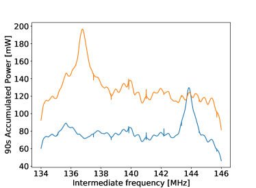
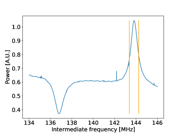
Figure 3: Left: Typical spectra for two different LO frequencies ($l1=8.240\,\mathrm{GHz}$ and $l2=8.247\,\mathrm{GHz}$). Upon changing the LO frequency, the cavity resonance peak changes position in the IF frequency. The visible spikes in the spectra are noisy bins produced by the improper isolation between the ADC card and the FPGA. Right: An example of a $\delta_{ij}^{d}$ spectrum obtained by the division of two spectra taken at two different LO frequencies. This procedure removes the wave-like structures originating from the electronics which are common to both spectra. The orange vertical lines represent the frequency range considered in the analysis which covers a region without noisy bins. The physical frequency (PF) of the input signal can be calculated using PF = IF + LO.

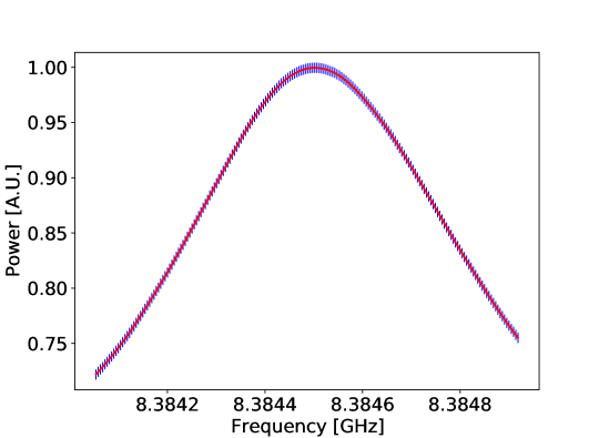
Figure 4: Typical 90 s spectrum after the division procedure. The blue vertical lines indicate the data points and the red line the SG-fit.The plotted frequency range corresponds to the region delimited by the two vertical lines in the right panel of figure 3.

The removal of the remaining structure is largely based on the HAYSTAC analysis procedure Brubaker:2017rna . A first Savitzky-Golay (SG) filter savitzky64 (with 15 points and a polynomial degree of 3) is applied to the average spectrum $\delta^{d}_{k}=(1/M)\sum_{i=1}^{M}\delta_{ik}^{d}$, producing a smoothed spectrum called SG-fit. This first SG filter removes the large structure originating from the electronics. Figure 4 shows a 90 s spectrum (blue vertical lines) and the SG-fit (in red) on top of it. The normalized spectra ($\delta_{ik}^{n}$) are obtained through dividing $\delta_{ik}^{d}$ by the SG-fit:

$$\delta_{ik}^{n}=\frac{\delta_{ik}^{d}}{\text{SG}_{k}}.$$ (6)

A second SG-fit ($\text{SG}^{*}$, produced using a SG-filter with 109 points and a polynomial degree of 3) has to be applied to each $\delta_{ik}^{n}$ to remove the effect of gain drifts and the normalized spectra are once again divided by these fits to obtain Unitless Normalized Spectra:

$$\delta_{ik}^{u}=\frac{\delta_{ik}^{n}}{\text{SG}_{ik}^{*}}-1.$$ (7)

In the absence of axion conversion and if appropriate SG parameters are used, these $\delta_{ik}^{u}$ should be samples of a Gaussian distribution center at $\mu$ = 0 and standard deviation $\sigma$ = $1/\sqrt{\Delta\nu\cdot t}$. Based on the transfer function of the SG filter, we optimized the parameters to achieve the aforementioned Gaussian distribution with the least impact on a possible axion signal. Figure 5 shows the histogram for all $\delta_{ik}^{u}$. The $\delta_{ik}^{u}$ are then combined into a Grand Unified Spectrum:

$$\delta_{k}^{g}=\frac{1}{M}\sum_{i=1}^{M}\delta_{ik}^{u},$$ (8)

with the sample variance:

$$(\sigma_{k}^{g})^{2}=\frac{1}{M-1}\sum_{i=1}^{M}(\delta_{ik}^{u}-\delta_{k}^{g})^{2}.$$ (9)

The distribution of the $\delta_{k}^{g}$ should also be fully Gaussian if the structures originating from the DAQ and other sources have been entirely removed. However, we observed a systematic deviation from the expected Gaussian distribution ($\mu$=0, $\sigma$=1). The obtained distribution fitted with a Gaussian yields $\mu=0.0\pm 0.2$ and $\sigma=1.7\pm 0.2$. We identified that magnet-on and magnet-off data exhibited similar features leading to a distribution in frequency that was not consistent with white noise. In order to remove the remaining structure, we subtracted the magnet-off data set ($\delta_{k}^{g\text{-off}}$, consisting of 30 h of data which were analyzed similarly to the magnet-on data) from $\delta_{k}^{g}$. Given the smaller sample size of the magnet-off data, this procedure increased the statistical uncertainty. By subtracting the two spectra, these features were removed and the resulting distribution was consistent with a Gaussian distributed white noise (see left panel of figure 6). We refer to this spectrum as the final Grand Unified Spectrum; $\delta_{k}^{f}$ = $\delta_{k}^{g}$ - $\delta_{k}^{g\text{-off}}$.

Figure 5:

Normalized histogram for all $\delta_{ik}^{u}$.

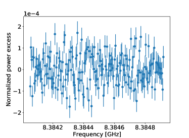
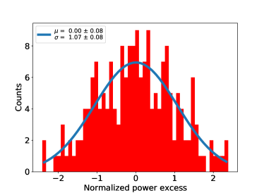
Figure 6: Left: Final Grand Unified Spectrum $\delta_{k}^{f}$ Right: normalized histogram of $\delta_{k}^{f}$.

An axion search using a fit based on an hypothetical axion line shape can be performed on $\delta_{k}^{f}$. The axion line shape was computed using the normalized velocity distribution function given in Turner:1990qx ; Brubaker:2017rna based of the standard isothermal spherical halo model:

$$f(\nu)=\frac{2}{\sqrt{\pi}}\left(\sqrt{\frac{3}{2}}\frac{1}{r}\frac{1}{\nu_{a}\langle\beta_{MB}^{2}\rangle}\right)\text{sinh}\left(3r\sqrt{\frac{2(\nu-\nu_{a})}{\nu_{a}\langle\beta_{MB}^{2}\rangle}}\right)\text{exp}\left(-\frac{3(\nu-\nu_{a})}{\nu_{a}\langle\beta_{MB}^{2}\rangle}-\frac{3r^{2}}{2}\right),$$ (10)

where $\nu_{a}$ is the Compton frequency of the axion field, $v_{s}$, the velocity of the Sun with respect to the Galaxy, and $\langle\beta_{MB}^{2}\rangle$ = $\langle v^{2}\rangle$/$c^{2}$ where $\langle v^{2}\rangle$ is the second moment of the Maxwell-Boltzmann distribution defined as $\langle v^{2}\rangle$ = 3$v_{c}^{2}$/2 = (270 km/s)², $r$ = $v_{s}$/$\sqrt{\langle v^{2}\rangle}\approx\sqrt{2/3}$ with $v_{s}\approx v_{c}=220\,\mathrm{km/s}$, the velocity of a terrestrial laboratory with respect to the rest frame of the galactic halo. A discretized version of the line shape is defined as:

$$L_{q}=\int_{\nu_{a}+(q-1)\Delta\nu}^{\nu_{a}+q\Delta\nu}f(\nu)d\nu,$$ (11)

where $\nu_{a}$ is the axion frequency and $q$ labels the bin number.

Given that the bin resolution bandwidth $\Delta\nu$ is 4577 Hz, equation (11) gives that $99\,\mathrm{\%}$ of the axion power should be deposited within 6 bins. Using a software-generated ’axion signal’, we studied the influence of the two SG-filters on the axion line shape which is distorted and attenuated by the filters. Correspondingly, a new resulting fit function ($y$) which accounts for this distortion and therefore spans a larger number of bins, was used in the search algorithm. A fit on 14 adjacent bins throughout $\delta_{k}^{f}$, using the following fit function, was performed:

$$y=A\cdot L^{d}_{q},$$ (12)

where $A$ (the free parameter in the fit) is the amplitude of the axion signal and $L^{d}_{q}$ is the distorted axion line shape. Figure 7 shows the value of $A$ obtained as a function of frequency, for frequency steps of $\Delta\nu$. The largest excess in the amplitude plot has a 3.67$\sigma$ local significance which corresponds to a 1.71$\sigma$ global significance after correcting for the look-elsewhere effect Lista:2017jsy . A search leaving $\nu_{a}$ as a free parameter within a bin width yielded the highest outlier at a global significance of 3.05$\sigma$ only. Thus no significant signal above statistical fluctuations was observed.

The Bayesian method was used to obtain an upper limit (UL). A flat prior function $\pi(A)=1$ for $A\geq 0$ and $\pi(A)=0$ for $A<0$ was used. The variable ($\delta_{k}^{f}$) being random Gaussian-distributed, the posterior function can be written as:

$$p(A,\delta_{k}^{f})=\frac{\text{e}^{-(S(\delta_{k}^{f},A)/2)}\pi(A)}{N},$$ (13)

where $N$ is the normalization factor. $S(\delta_{k}^{f},A)$ is defined as:

$$S(\delta_{k}^{f},A)=\sum_{k}\left(\frac{(\delta_{k}^{f}-y(k,A))^{2}}{\sigma_{k}^{2}}\right),$$ (14)

where $\sigma_{k}$ is the uncertainty on $\delta_{k}^{f}$.

Finally, to compute the upper limit we use:

$$\frac{1}{N}\int_{0}^{A_{\text{UL}}}\text{e}^{-(\sum_{k}S(\delta_{k}^{f},A)/2)}dA=1-\alpha,$$ (15)

where 1 - $\alpha$ is the credibility level (CL) of the UL. For this analysis a 95$\%$ CL was used. The black solid line of figure 8 shows the upper limit obtained from our measurement. This result has to be compared to the expected UL given the expected noise fluctuations. A large number of simulated spectra (1000) with the expected white noise fluctuations were created. The expected noise fluctuation (5.14$\times 10^{-5}$) is calculated using the error propagation formula for the subtraction of the two spectra. The expected uncertainty for the magnet-on and magnet-off data can be computed using $\sigma=1/\sqrt{\Delta\nu\cdot t}$. The UL was computed for each one of these spectra using equation (15). The dotted red line of figure 8 shows the average expected UL and corresponding uncertainty bands. The bands were calculated by integrating numerically the histogram of the UL distribution of the simulated spectra. We note that the bands are not symmetric because of the choice of the prior.

We translate the normalized upper limits into power values by multiplying them with the noise power. Using equation (1) and (2) we obtain an exclusion limit of g${}_{a\gamma}\gtrsim 4\times 10^{-13}\,\mathrm{GeV^{-1}}$ within $34.6738\,\mathrm{\mu eV}<m_{a}<34.6771\,\mathrm{\mu eV}$. The level of systematic uncertainties is assessed by error propagation of the experimentally determined physical quantities involved in equation (1). Those uncertainties are represented as the green band in the insert of Figure 9. They account for less than $10\,\mathrm{\%}$ error, dominated by the knowledge of the noise temperature, and were thus neglected in the estimation of the exclusion limit.

Figure 9 shows the result of this analysis in the context of other haloscope searches: CAST-RADES places a competitive limit at an axion mass above the highest
ADMX-Sidecar limit Boutan:2018uoc and slightly lower than the QUAX results Alesini:2019ajt ; Alesini:2020vny .

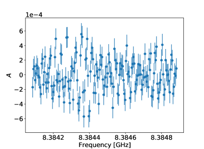
Figure 7: Amplitude $A$ (in units of normalized power excess) of the axion signal provided by the fit for each of the probed axion frequencies.

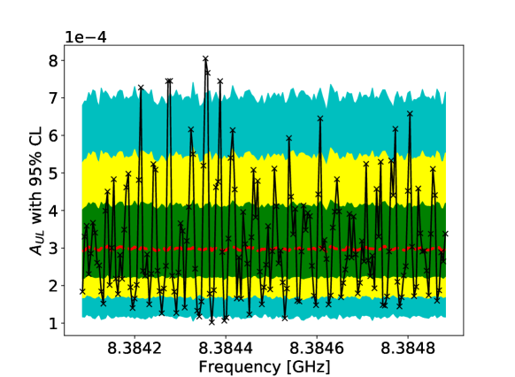
Figure 8:

Observed (solid black line) and expected (dotted red line) of $A_{\text{UL}}$ (in units of normalized power excess) for 95$\%$ CL and the 1, 2 and 3 $\sigma$ bands for the background-only hypothesis.

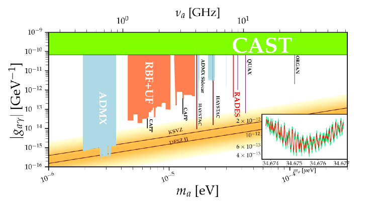
Figure 9: Axion-photon coupling versus axion mass phase-space. In dark red the CAST-RADES axion-photon coupling exclusion limit with 95$\%$ credibility level presented in this manuscript. The coupling-mass plane is shown in natural units for consistency with most literature in the field. Other haloscope results: RBF DePanfilis:1987dk , UF Hagmann:1990tj , ADMX and ADMX-SideCar Braine:2019fqb ; Du:2018uak ; Boutan:2018uoc , CAPP Lee:2020cfj ; Jeong:2020cwz , HAYSTAC Zhong:2018rsr ; Backes:2020ajv , QUAX Alesini:2019ajt ; Alesini:2020vny and ORGAN McAllister:2017lkb and the CAST solar axion results Anastassopoulos:2017ftl are plotted for comparison, see ohare for a full list of references and the raw source for the plot. Inset: Zoom-in of the parameter range probed in this work ($34.6738\,\mathrm{\mu eV}<m_{a}<34.6771\,\mathrm{\mu eV}$), where the green region represent the uncertainty of the measurement.

4 Conclusion and prospects

Well-founded theoretical motivations suggest to search for axion masses above 25 $\mu$eV. However, a challenge in the path to probe higher masses using RF cavities to search for axions in the galactic halo is that the effective volume of the cavity tends to decrease with increasing frequencies. This work demonstrates for the first time the possibility of searching for an axion signal at masses above 30 $\mu$eV using a rectangular cavity segmented by irises. The result for an axion search at 34.67 $\mu$eV is presented; no signal above noise was found in the data set. The extracted upper limit of the axion-photon coupling for a narrow frequency band improves the previous CAST limit Anastassopoulos:2017ftl at the corresponding axion mass by more than 2 orders of magnitude.

This investigation constitutes the first data-taking campaign of CAST-RADES. Currently, a 1-m long cavity with alternating cavities is taking data in the CAST magnet, see Melcon:2020xvj for details. Further R&D avenues of RADES, like mechanical and ferro-electric tuning as well as tests with superconducting cavities are underway.

References

- [1] P.A.R. Ade et al. Planck 2015 results. XIII. Cosmological parameters. Astron. Astrophys., 594:A13, 2016.
- [2] G. Bertone, D. Hooper, and J. Silk. Particle dark matter: Evidence, candidates and constraints. Phys. Rept., 405:279–390, 2005.
- [3] D. Clowe et al. A direct empirical proof of the existence of dark matter. Astrophys. J. Lett., 648:L109–L113, 2006.
- [4] S. Weinberg. A new light boson? Phys. Rev. Lett., 40:223–226, Jan 1978.
- [5] F. Wilczek. Problem of strong and invariance in the presence of instantons. Phys. Rev. Lett., 40:279–282, Jan 1978.
- [6] R.D. Peccei and H.R. Quinn. conservation in the presence of pseudoparticles. Phys. Rev. Lett., 38:1440–1443, Jun 1977.
- [7] R.D. Peccei and H.R. Quinn. Constraints imposed by conservation in the presence of pseudoparticles. Phys. Rev. D, 16:1791–1797, Sep 1977.
- [8] L.F. Abbott and P. Sikivie. A Cosmological Bound on the Invisible Axion. Phys. Lett. B, 120:133–136, 1983.
- [9] M. Dine and W. Fischler. The Not So Harmless Axion. Phys. Lett. B, 120:137–141, 1983.
- [10] M. Tanabashi et al. Review of particle physics. Phys. Rev. D, 98:030001, Aug 2018.
- [11] M. Kawasaki, K. Saikawa, and T. Sekiguchi. Axion dark matter from topological defects. Phys. Rev. D, 91:065014, Mar 2015.
- [12] L. Fleury and Guy D. Moore. Axion dark matter: strings and their cores. JCAP, 01:004, 2016.
- [13] P. Agrawal et al. Experimental Targets for Photon Couplings of the QCD Axion. JHEP, 02:006, 2018.
- [14] L. Di Luzio, F. Mescia, and E. Nardi. Redefining the Axion Window. Phys. Rev. Lett., 118(3):031801, 2017.
- [15] P. Arias et al. WISPy Cold Dark Matter. JCAP, 06:013, 2012.
- [16] I. G. Irastorza and J. Redondo. New experimental approaches in the search for axion-like particles. Prog. Part. Nucl. Phys., 102:89–159, 2018.
- [17] H. Primakoff. Photoproduction of neutral mesons in nuclear electric fields and the mean life of the neutral meson. Phys. Rev., 81:899, 1951.
- [18] P. Sikivie. Experimental Tests of the Invisible Axion. Phys. Rev. Lett., 51:1415–1417, 1983. [Erratum: Phys.Rev.Lett. 52, 695 (1984)].
- [19] L. Krauss et al. Calculations for Cosmic Axion Detection. Phys. Rev. Lett., 55:1797, 1985.
- [20] S. Al Kenany et al. Design and operational experience of a microwave cavity axion detector for the 20–100 eV range. Nucl. Instrum. Meth. A, 854:11–24, 2017.
- [21] J. I. Read. The Local Dark Matter Density. J. Phys. G, 41:063101, 2014.
- [22] R.H. Dicke. The Measurement of Thermal Radiation at Microwave Frequencies. Rev. Sci. Instrum., 17(7):268–275, 1946.
- [23] N. Du et al. A Search for Invisible Axion Dark Matter with the Axion Dark Matter Experiment. Phys. Rev. Lett., 120(15):151301, 2018.
- [24] T. Braine et al. Extended Search for the Invisible Axion with the Axion Dark Matter Experiment. Phys. Rev. Lett., 124(10):101303, 2020.
- [25] L. Zhong et al. Results from phase 1 of the HAYSTAC microwave cavity axion experiment. Phys. Rev. D, 97(9):092001, 2018.
- [26] S. Lee et al. Axion Dark Matter Search around 6.7 eV. Phys. Rev. Lett., 124(10):101802, 2020.
- [27] J. Jeong et al. Concept of multiple-cell cavity for axion dark matter search. Phys. Lett. B, 777:412–419, 2018.
- [28] J. Jeong et al. Search for Invisible Axion Dark Matter with a Multiple-Cell Haloscope. Phys. Rev. Lett., 125(22):221302, 2020.
- [29] O.K. Baker et al. Prospects for Searching Axion-like Particle Dark Matter with Dipole, Toroidal and Wiggler Magnets. Phys. Rev. D, 85:035018, 2012.
- [30] V. Anastassopoulos et al. New CAST Limit on the Axion-Photon Interaction. Nature Phys., 13:584–590, 2017.
- [31] A.A. Melcón et al. Axion Searches with Microwave Filters: the RADES project. JCAP, 05:040, 2018.
- [32] A. Caldwell et al. Dielectric Haloscopes: A New Way to Detect Axion Dark Matter. Phys. Rev. Lett., 118(9):091801, 2017.
- [33] BRASS collaboration. https://www.physik.uni-hamburg.de/en/iexp/gruppe-horns/forschung/brass.html. Accessed: 13-04-2021.
- [34] D. Alesini et al. Galactic axions search with a superconducting resonant cavity. Phys. Rev. D, 99(10):101101, 2019.
- [35] D. Alesini et al. Search for Invisible Axion Dark Matter of mass meV with the QUAX– Experiment. 12 2020.
- [36] B. T. McAllister et al. The ORGAN Experiment: An axion haloscope above 15 GHz. Phys. Dark Univ., 18:67–72, 2017.
- [37] K. M. Backes et al. A quantum-enhanced search for dark matter axions. Nature Phys., 590(7845):238–242, 2021.
- [38] CST Microwave Studio Suite. www.3ds.com. Accessed: 25-08-2020.
- [39] David M Pozar. Microwave engineering; 3rd ed. Wiley, Hoboken, NJ, 2005.
- [40] Keysight Technologies. Application Note 5952-3706E (2019). https://www.keysight.com/ch/de/assets/7018-06829/application-notes/5952-3706.pdf.
- [41] B. M. Brubaker et al. Haystac axion search analysis procedure. Phys. Rev. D, 96:123008, Dec 2017.
- [42] A. Savitzky and M. J. E. Golay. Smoothing and differentiation of data by simplified least squares procedures. Anal. Chem., 36:1627–1639, 1964.
- [43] M. S. Turner. Periodic signatures for the detection of cosmic axions. Phys. Rev. D, 42:3572–3575, Nov 1990.
- [44] L. Lista. Statistical Methods for Data Analysis in Particle Physics, volume 941. Springer, 2017.
- [45] C. Boutan et al. Piezoelectrically tuned multimode cavity search for axion dark matter. Phys. Rev. Lett., 121, 12 2018.
- [46] S. De Panfilis et al. Limits on the Abundance and Coupling of Cosmic Axions at 4.5-Microev m(a) 5.0-Microev. Phys. Rev. Lett., 59:839, 1987.
- [47] C. Hagmann et al. Results from a search for cosmic axions. Phys. Rev. D, 42:1297–1300, 1990.
- [48] C. O’HARE. Axion limits. https://github.com/cajohare/AxionLimits/.
- [49] A. Álvarez Melcón et al. Scalable haloscopes for axion dark matter detection in the 30eV range with RADES. JHEP, 07:084, 2020.