A Note on Connecting Barlow Twins with
Negative-Sample-Free Contrastive Learning

Barlow Twins (Zbontar et al., 2021) is a recently proposed self-supervised learning (SSL) method that encourages similar representations between distorted variations (augmented views) of a sample, while minimizing the redundancy within the representation vector. Specifically, compared to the prior state-of-the-art SSL methods, Barlow Twins demonstrates two main properties. On one hand, its algorithm requires no explicit construction of negative sample pairs, and is not sensitive to large training batch sizes, both of which are the characteristics commonly seen in the recent non-contrastive SSL methods (e.g., BYOL (Grill et al., 2020) and SimSiam (Chen and He, 2020)). On the other hand, it avoids the reliance on symmetry-breaking network designs for distorted samples, which had been found to be crucial for these non-contrastive approaches (in order to avoid learning collapsed representations). We note that designing symmetry-breaking networks is not needed for the recent contrastive SSL methods (e.g., SimCLR (Chen et al., 2020)). A natural question arises: what makes Barlow Twins an outlier among the existing SSL algorithms?

Zbontar et al. (2021) motivated the algorithmic design of Barlow Twins via the Information Bottleneck (IB) theory (Tishby et al., 2000), assuming the representations are Gaussian and that we need to minimize the determinant of the feature cross-correlation. In this note we provide an alternative interpretation of the Barlow Twins’ objective by viewing it as a negative-sample-free contrastive learning objective. Specifically, we relate the method to Hilbert-Schmidt Independence Criterion (HSIC) (Gretton et al., 2005) maximization between augmented views, where HSIC is a contrastive approach that avoids the need of constructing negative pairs. We show that this new interpretation entails no assumption on the Gaussianity, and is thus more consistent with how Barlow Twins is used in practice. While the HSIC interpretation calls for a slight change to the original Barlow Twins’ objective, we empirically show that the change leads to no loss in performance.

Overall, we believe that such negative-sample-free contrastive approach (exemplified by Barlow Twins) can serve as a bridge between the two major families of SSL methods: non-contrastive (e.g., BYOL (Grill et al., 2020), SimSiam (Chen and He, 2020)) and contrastive approaches (e.g., SimCLR (Chen et al., 2020)).

1 Barlow Twins’ Method

We first obtain the distorted variations of a given sample by applying different augmentations (i.e., Gaussian blurring, rotation, translation, etc.). Then, Barlow Twins’ method (Zbontar et al., 2021) encourages the empirical cross-correlation matrix (between learned representations of the distorted variations of a given sample) to be an identity matrix. The rationale is that 1) when on-diagonal terms of the cross-correlation matrix take value $+1$, it encourages the learned representations of distorted versions of a sample to be similar; and 2) when off-diagonal terms of the cross-correlation matrix take value $0$, it encourages the diversity of learned representations, since different dimensions of these representations will be uncorrelated to each other.

For notations simplicity, throughout the report, we assume $X\in\mathbb{R}^{n\times d}$ and $Y\in\mathbb{R}^{n\times d}$ to be standardized features (mean zero and standard deviation one) from the distorted versions of a given sample. To be more precise,

$$X={\rm Standardization\Big{(}Feature\_Encoder\big{(}Augmented\_Data\_1\big{)}\Big{)}}$$

and

$$Y={\rm Standardization\Big{(}Feature\_Encoder\big{(}Augmented\_Data\_2\big{)}\Big{)}}.$$

$n$ is the number of samples and $C$ = $\frac{X^{\top}Y}{n}\in\mathbb{R}^{d\times d}$ is the empirical cross-correlation matrix. Barlow Twin’s objective considers the following loss:

$${\rm Barlow\,\,Twins^{\prime}\,\,Loss\,\,}=\,\sum_{i}(1-C_{ii})^{2}+\lambda\sum_{i}\sum_{j\neq i}C_{ij}^{2},$$ (1)

where $\lambda$ is a trade-off parameter controlling the on- (i.e., $C_{ii}$) and off-diagonal terms (i.e., $C_{ij}$ for $i\neq j$). In Zbontar et al. (2021), the authors find that $\lambda=0.005$ works the best using a grid search.

2 Hilbert-Schmidt Independence Criterion for Self-supervised Learning

We denote $P_{XY}$ and $P_{X}P_{Y}$ as the joint and the product of marginal distributions of the features $X$ and $Y$. Contrastive learning objectives (Chen et al., 2020; Hjelm et al., 2018; Ozair et al., 2019; Tsai et al., 2021a) aim to learn similar representations for positively paired data (i.e., $x$ would be similar to $y$ when $(x,y)\sim P_{XY}$) and learning dissimilar representations for negatively paired data (i.e., $x$ would be dissimilar to $y$ when $(x,y)\sim P_{X}P_{Y}$). For example, $P_{XY}$ denotes the distribution of learned representations from distorted variations of a given sample and $P_{X}P_{Y}$ denotes the distribution of learned representations from different samples. Tsai et al. (2021a) showed that the contrastive objectives can be interpreted as maximizing the probability divergence between $P_{XY}$ and $P_{X}P_{Y}$, where the probability divergence can be either Kullback–Leibler divergence (Chen et al., 2020), Jensen–Shannon divergence (Hjelm et al., 2018), Wasserstein divergence  (Ozair et al., 2019) or $\chi^{2}$ divergence (Tsai et al., 2021a). Hilbert-Schmidt Independence Criterion (HSIC) (Gretton et al., 2005) also represents a probability divergence between $P_{XY}$ and $P_{X}P_{Y}$, where it considers the maximum mean discrepancy (MMD) (Gretton et al., 2012) as the probability divergence measurement. In particular,

$${\rm HSIC}(X,Y):={\rm MMD}\,(\,P_{XY}\,\|\,P_{X}P_{Y}\,)=\|C_{XY}\|_{\rm HS}^{2},$$ (2)

where $C_{XY}$ is the cross-covariance operators between the Reproducing Kernel Hilbert Spaces (RKHSs) of $X$ and $Y$ and $\|\cdot\|_{\rm HS}^{2}$ is the Hilbert-Schmidt norm. Gretton et al. (2005) proposed an empirical estimation of HSIC:

$$\widehat{{\rm HSIC}(X,Y)}:=\frac{1}{n^{2}}\,{\rm tr}\,\Big{(}{\bf K_{X}HK_{Y}H}\Big{)},$$ (3)

where ${\bf K_{X}}$ and ${\bf K_{Y}}$ are kernel Gram matrices of $X$ and $Y$ respectively and ${\bf H}={\bf I}-\frac{1}{n}{\bf 1}{\bf 1}^{\top}\in\mathbb{R}^{n\times n}$ is the centering matrix. We note that the above equation only requires the positively paired samples to construct the kernel ${\bf K_{X}}$ and ${\bf K_{Y}}$. Hence, adopting HSIC as a contrastive learning objective avoids the need of explicitly minimizing the similarities between the negatively paired data, which is crucial in prior contrastive learning methods (Chen et al., 2020; Hjelm et al., 2018; Ozair et al., 2019; Tsai et al., 2021a). In short, HSIC objective can be interpreted as a negative-sample-free contrastive learning objective. In what follows, we will show that by considering the linear kernel as the characteristic kernel in the RKHSs, we can relate HSIC objective to the Barlow Twins’ objective.

2.1 Connecting HSIC to Barlow Twins

To connect HSIC to Barlow Twins, we let the characteristic kernel in the RKHSs to be the linear kernel, in particular ${\bf K_{X}}=XX^{\top}$ and ${\bf K_{Y}}=YY^{\top}$. Since $X$ and $Y$ are standardized (mean $0$), it is not hard to show that $XX^{\top}{\bf H}=XX^{\top}$ and $YY^{\top}{\bf H}=YY^{\top}$. Plugging in this result into equation (3), we obtain:

$$\begin{split}\widehat{{\rm HSIC}(X,Y)}:=&\frac{1}{n^{2}}\,{\rm tr}\,\Big{(}{\bf K_{X}HK_{Y}H}\Big{)}=\frac{1}{n^{2}}\,{\rm tr}\,\Big{(}XX^{\top}YY^{\top}\Big{)}\\ =&\frac{1}{n^{2}}\,{\rm tr}\,\Big{(}X^{\top}Y\big{(}X^{\top}Y\big{)}^{\top}\Big{)}=\frac{1}{n^{2}}\|X^{\top}Y\|_{F}^{2}=\|C\|_{F}^{2},\end{split}$$ (4)

where $C$ is the empirical cross-correlation matrix by definition and $\|\cdot\|_{F}^{2}$ is the Frobenius norm. We see that, when considering the linear kernel (i.e., $k(x,y)=\langle\,x,y\rangle$), the Hilbert-Schmidt norm of the cross-covariance operator in equation (2) equals to the Frobenius norm of the cross-covariance matrix. And we note that, since $X$ and $Y$ are standardized, the cross-covariance matrix becomes the cross-correlation matrix, where $C_{ij}\in[-1,1]\,\,\forall\,i,j\in\{1,\cdots,d\}$.

Contrastive learning approaches aim to maximize the distribution divergence between $P_{XY}$ and $P_{X}P_{Y}$, which means that we can maximize equation (4) for self-supervised representation learning. Nonetheless, a trivial solution $C_{ij}=1\,\,\forall\,i,j\in\{1,\cdots,d\}$ exists when maximizing equation (4), which is not ideal since the perfect correlation ($+1$) between different dimensions of the representations implies a low power of the representations. By noticing that $C_{ij}=+1$ or $C_{ij}=-1$ both maximizes $C_{ij}^{2}$, we can prevent this trivial solution by encouraging 1) the on-diagonal terms of $C$ to be $+1$ and 2) the off-diagonal terms of $C$ to be $-1$. Then, the resulting loss is:

$${\rm HSIC_{\rm ssl}\,\,}=\,\sum_{i}(1-C_{ii})^{2}+\lambda\sum_{i}\sum_{j\neq i}(1+C_{ij})^{2},$$ (5)

where $\lambda$ is a trade-off hyper-parameter. Equation (5) resembles the original Barlow Twins’ objective (equation (1)) with the difference on the off-diagonal terms: Barlow Twins encourages the off-diagonal terms to be zero and the ${\rm HSIC_{\rm SSL}}$ encourages the off-diagonal terms to be negative one.

2.2 Discussion

Connecting ${\rm HSIC_{\rm SSL}}$ to downstream tasks: So far we see that minimizing ${\rm HSIC_{\rm SSL}}$ (equation (5)) encourages the dependency between learned representations from the distorted samples (i.e., $X$ and $Y$). Maximizing this dependency can be viewed as maximizing the mutual information between learned representations, where Tsai et al. (2021b) showed that this process acts to extract downstream task-relevant information. A complementary objective to extracting downstream-task-relevant information is the objective that discards downstream-task-irrelevant information, such as the squared loss between $X$ and $Y$ (i.e., $\|X-Y\|_{F}^{2}$, see Tsai et al. (2021b)). We will show that minimizing the squared loss between $X$ and $Y$ equals to encouraging the on-diagonals of $C$ to be $+1$:

$$\begin{split}\|X-Y\|_{F}^{2}&={\rm tr}\Big{(}\big{(}X-Y\big{)}^{\top}\big{(}X-Y\big{)}\Big{)}={\rm tr}\Big{(}X^{\top}X+Y^{\top}Y-X^{\top}Y-Y^{\top}X\Big{)}\\ &=2d-2{\rm tr}\Big{(}X^{\top}Y\Big{)}=2d-2n\,{\rm tr}\Big{(}C\Big{)},\end{split}$$ (6)

where $X^{\top}X=Y^{\top}Y=d$ because $X$ and $Y$ are standardized representations. Since the cross-correlation ranges between $-1$ and $+1$, maximizing ${\rm tr}\,\big{(}C\big{)}$ encourages the on-diagonal entries of $C$ to be $+1$. To conclude, ${\rm HSIC_{\rm SSL}}$ (equation (5)) plays the role to both extract downstream-task-relevant (i.e., maximizing the mutual information between $X$ and $Y$) and discard downstream task-irrelevant information (i.e., minimizing the squared loss between $X$ and $Y$).

The choice of $\lambda$: As suggested by Zbontar et al. (2021), one can find $\lambda$ by a grid search. Another choice is to set $\lambda=\frac{1}{d}$ since we want to balance on-diagonal and off-diagonal terms in equation (5). Note that equation (5) contains $d$ on-diagonal terms and $d\cdot(d-1)$ off-diagonal terms, and the ratio is $\frac{1}{d-1}\approx\frac{1}{d}$. We empirically find this choice of $\lambda$ to work well when altering the dimension $d$, either for the Barlow Twins’ method (equation (1)) or ${\rm HSIC_{\rm SSL}}$ (equation (5)).

3 Experiments

The experiments considered in this technical report serves to fairly compare the Barlow Twins’ loss (equation (1)) and ${\rm HSIC_{\rm SSL}}$ (equation (5)), where we will later show that there is negligible performance difference between these two objective functions. Throughout the experiments, we set $\lambda=\frac{1}{d}$ in both the Barlow Twins’ loss and ${\rm HSIC_{\rm SSL}}$ with $d$ being the dimension of the features. We choose CIFAR-10 (Krizhevsky et al., 2009) and Tiny-Imagenet (Le and Yang, 2015) as our datasets.

Training and Evaluation.

We choose ResNet-50 (He et al., 2016) as our backbone model (serving as the encoder described in (Chen et al., 2020)) and replace the last classification layer with a non-linear projection layer (serving as the projection head described in (Chen et al., 2020)). The encoder takes the input of an image and outputs a $2048$-dimensional feature. The projection head takes the input of the $2048$-dimensional feature and outputs a $d$-dimensional feature. Both the Barlow Twins’s loss and ${\rm HSIC_{\rm SSL}}$ consider the $d$-dimensional features as $X$ and $Y$. During training, we update the parameters in the encoder and the projection head to minimize the chosen loss, $1,000$ epochs on CIFAR10 and $650$ epochs on Tiny ImageNet. The inputs are distorted variations of input samples. During evaluation, we remove the projection head and report the metric on the test images using the $2048$-dimensional feature with the linear classification (Chen et al., 2020) accuracy. The linear classification approach categorizes test images by additionally training another linear classifier on top of the $2048$-dimensional features, $200$ epochs for both datasets. More details can be found in https://github.com/yaohungt/Barlow-Twins-HSIC.

Results and Discussions.

First, in Figure 1, we compare the learned self-supervised representations on CIFAR10 and Tiny ImageNet by changing the projector dimension $d$. The batch size is fixed to $128$ and $\lambda$ is set to be $\frac{1}{d}$. We find that the performance difference between Barlow Twins and ${\rm HSIC_{\rm SSL}}$ is negligible. We also find that the performance does not differ much when altering $d$. This observation has a conflict with the original Barlow Twins’ paper (Zbontar et al., 2021), where it states that the Barlow Twins’ method performs better when the projector dimension $d$ is large (see its Figure 4). We argue that this disaccordance is because of 1) the self-supervised learned representations behave differently on large datasets (ImageNet considered by Zbontar et al. (2021)) and small datasets (CIFAR10 and Tiny ImageNet considered by us); and 2) the choice of $\lambda$ (we set $\lambda=\frac{1}{d}$, and it is unclear that has $\lambda$ be chosen by extensively grid search in Figure 4 in the paper (Zbontar et al., 2021)).

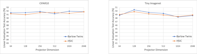
Figure 1: Comparisons of the learned self-supervised representations on CIFAR10 and Tiny ImageNet by changing the projector dimension $d$. The batch size is fixed to $128$ and $\lambda$ is set to be $\frac{1}{d}$.

Second, in Figure 2, we compare the learned self-supervised representations on CIFAR10 by changing the number of training epochs and effect of batch size. The projector dimension is fixed to $128$ and $\lambda$ is set to be $\frac{1}{128}$. The same trend is observed: we do not find obvious performance difference between Barlow Twins and ${\rm HSIC_{\rm SSL}}$. Another interesting observation is that Barlow Twins and ${\rm HSIC_{\rm SSL}}$ reach to worsened performance when increasing the batch size. This observation has also be found in Figure 2 in the original Barlow Twins’ paper (Zbontar et al., 2021). We do not have a good explanation for this phenomenon and will continue on investigating it.

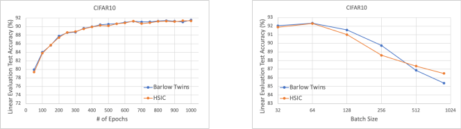
Figure 2: Comparisons of the learned self-supervised representations on CIFAR10 by changing the number of training epochs and effect of batch size. The projector dimension is fixed to $128$ and $\lambda$ is set to be $\frac{1}{128}$.

4 Conclusion

In this report, we relate the algorithmic design of Barlow Twins’ method (Zbontar et al., 2021) to the Hilbert-Schmidt Independence Criterion (HSIC), thus establishing it as a contrastive learning approach that is free of negative samples. Through this perspective, we argue that Barlow Twins (and thus the class of negative-sample-free contrastive learning methods) suggests a possibility to bridge the two major families of self-supervised learning philosophies: non-contrastive and contrastive approaches. In particular, Barlow twins exemplified how we could combine the best practices of both worlds: avoiding the need of large training batch size and negative sample pairing (like non-contrastive methods) and avoiding symmetry-breaking network designs (like contrastive methods). To conclude, we believe this work sheds light on the advantage of exploring the directions of designing negative-sample-free contrastive learning objectives.

References

- Chen et al. (2020) Ting Chen, Simon Kornblith, Mohammad Norouzi, and Geoffrey Hinton. A simple framework for contrastive learning of visual representations. In International conference on machine learning, pages 1597–1607. PMLR, 2020.
- Chen and He (2020) Xinlei Chen and Kaiming He. Exploring simple siamese representation learning. arXiv preprint arXiv:2011.10566, 2020.
- Gretton et al. (2005) Arthur Gretton, Olivier Bousquet, Alex Smola, and Bernhard Schölkopf. Measuring statistical dependence with hilbert-schmidt norms. In Proceedings of the 16th international conference on Algorithmic Learning Theory, pages 63–77, 2005.
- Gretton et al. (2012) Arthur Gretton, Karsten M Borgwardt, Malte J Rasch, Bernhard Schölkopf, and Alexander Smola. A kernel two-sample test. The Journal of Machine Learning Research, 13(1):723–773, 2012.
- Grill et al. (2020) Jean-Bastien Grill, Florian Strub, Florent Altché, Corentin Tallec, Pierre H Richemond, Elena Buchatskaya, Carl Doersch, Bernardo Avila Pires, Zhaohan Daniel Guo, Mohammad Gheshlaghi Azar, et al. Bootstrap your own latent: A new approach to self-supervised learning. arXiv preprint arXiv:2006.07733, 2020.
- He et al. (2016) Kaiming He, Xiangyu Zhang, Shaoqing Ren, and Jian Sun. Deep residual learning for image recognition. In Proceedings of the IEEE conference on computer vision and pattern recognition, pages 770–778, 2016.
- He et al. (2020) Kaiming He, Haoqi Fan, Yuxin Wu, Saining Xie, and Ross Girshick. Momentum contrast for unsupervised visual representation learning. In Proceedings of the IEEE/CVF Conference on Computer Vision and Pattern Recognition, pages 9729–9738, 2020.
- Hjelm et al. (2018) R Devon Hjelm, Alex Fedorov, Samuel Lavoie-Marchildon, Karan Grewal, Phil Bachman, Adam Trischler, and Yoshua Bengio. Learning deep representations by mutual information estimation and maximization. arXiv preprint arXiv:1808.06670, 2018.
- Krizhevsky et al. (2009) Alex Krizhevsky, Geoffrey Hinton, et al. Learning multiple layers of features from tiny images. 2009.
- Le and Yang (2015) Ya Le and Xuan Yang. Tiny imagenet visual recognition challenge. CS 231N, 7:7, 2015.
- Ozair et al. (2019) Sherjil Ozair, Corey Lynch, Yoshua Bengio, Aaron van den Oord, Sergey Levine, and Pierre Sermanet. Wasserstein dependency measure for representation learning. arXiv preprint arXiv:1903.11780, 2019.
- Tishby et al. (2000) Naftali Tishby, Fernando C Pereira, and William Bialek. The information bottleneck method. arXiv preprint physics/0004057, 2000.
- Tsai et al. (2021a) Yao-Hung Hubert Tsai, Martin Q Ma, Muqiao Yang, Han Zhao, Louis-Philippe Morency, and Ruslan Salakhutdinov. Self-supervised representation learning with relative predictive coding. arXiv preprint arXiv:2103.11275, 2021a.
- Tsai et al. (2021b) Yao-Hung Hubert Tsai, Yue Wu, Ruslan Salakhutdinov, and Louis-Philippe Morency. Self-supervised learning from a multi-view perspective. In ICLR, 2021b.
- Zbontar et al. (2021) Jure Zbontar, Li Jing, Ishan Misra, Yann LeCun, and Stéphane Deny. Barlow twins: Self-supervised learning via redundancy reduction. arXiv preprint arXiv:2103.03230, 2021.