Optimal Transport between Gaussian random fields

Abstract

We consider the optimal transport problem between zero mean Gaussian stationary random fields both in the aperiodic and periodic case. We show that the solution corresponds to a weighted Hellinger distance between the multivariate and multidimensional power spectral densities of the random fields. Then, we show that such a distance defines a geodesic, which depends on the weight function, on the manifold of the multivariate and multidimensional power spectral densities.

I Introduction

The Optimal Transport Problem (OTP) aims in minimizing the effort to transport one nonnegative measure to another nonnegative measure according to a cost of moving mass from a point to another one. This problem has been formulated by Kantorovitch [1] and in the recent years it has been used for deriving new distances between covariance matrices and spectral densities, [2, 3, 4, 5, 6]. In particular, in [7] it has been shown that the OTP between Gaussian stationary stochastic processes leads to weighted Hellinger distance between multivariate and unidimensional power spectral densities. The latter distance is a generalization of the Hellinger distance introduced in [8, 9].

Distances between spectral densities play a fundamental role in spectral analysis. Indeed, the latter can be used in order to design high resolution spectral estimators [10, 11, 12, 13, 14] as well the multivariate extensions [15, 16, 17, 18, 19, 20]. These methods have been extended to: 1) stationary (i.e. homogeneous) random fields which are characterized by multidimensional power spectral densities [21, 22, 23, 24]; 2) stationary periodic random fields which are characterized by multidimensional power spectral densities whose domain is constituted by a finite number of points [25, 26]. It is worth noting that in the unidimensional case, the latter case boils down to the so called reciprocal processes, [27, 28, 29, 30, 31].

The aim of this paper is to extend the results in [7] to Gaussian stationary aperiodic/periodic random fields. More precisely, we formulate the OTP and we show that the corresponding solution is a suitable weighted Hellinger distance between multivariate and multidimensional spectral densities. Moreover, we show this distance defines a geodesic on the manifold of the multidimensional power spectral densities. The latter can be used in order to perform spectral morphing [32] for describing a Gaussian random field whose description slowly varies over time.

The outline of the paper is the following. In Section II we introduce the OTP for Gaussian random fields. In Section III we introduce the OTP for Gaussian periodic random fields. Section IV regards the spectral morphing problem and in Section V we present a numerical example. In Section VI we discuss the general case, i.e. the Gaussian assumption is not required. Finally, some conclusions are drawn in Section VII.

Notation: $\mathbb{R}$, $\mathbb{Z}$, $\mathbb{N}$ denote the set of real, integer and natural numbers, respectively. Given two vectors $\bm{\alpha}$ and $\bm{\vartheta}$ of the same dimension, then $\langle\bm{\alpha},\bm{\vartheta}\rangle$ denotes their inner product. Let $A$ be an Hermitian matrix, then $A>0$ ($A\geq 0$) means that $A$ is positive (semi)definite; $A^{*}$ denotes its transposed and conjugate. Moreover, we will consider the Euclidean norms $\|A\|:=\sqrt{\operatorname{tr}(A^{*}A)}$ and $\|A\|_{W}:=\sqrt{\operatorname{tr}(A^{*}WA)}$ with $W=W^{*}>0$. Given a function $\Phi(e^{j\bm{\vartheta}})$ with $\mathbb{T}^{d}:=[0,2\pi]^{d}$, such that $\Phi(e^{j\bm{\vartheta}})=\Phi(e^{j\bm{\vartheta}})^{*}$, then $\Phi>0$ ($\Phi\geq 0$) means that $\Phi(e^{j\bm{\vartheta}})>0$ ($\Phi(e^{j\bm{\vartheta}})\geq 0$) for any $\bm{\vartheta}\in\mathbb{T}^{d}$. $\ell_{1}^{m\times m}(\mathbb{Z}^{d})$ is the space of sequences $\mathbf{h}:=\{\,H_{\mathbf{t}},\;\mathbf{t}\in\mathbb{Z}^{d}\,\}$, with $H_{\mathbf{t}}\in\mathbb{R}^{m\times m}$, which are absolutely summable. Given two sequences $\mathbf{h}$ and $\mathbf{v}$, then $\mathbf{h}\star\mathbf{v}$ denotes the discrete convolution operation.

II OTP between random fields

Consider two jointly Gaussian stationary random fields $\mathbf{x}=\{\mathbf{x}_{\mathbf{t}},\;\mathbf{t}\in\mathbb{Z}^{d}\}$ and $\mathbf{y}=\{\mathbf{y}_{\mathbf{t}},\;\mathbf{t}\in\mathbb{Z}^{d}\}$ having zero mean and taking values in $\mathbb{R}^{m}$. It is worth noting that the index $\mathbf{t}=(t_{1},t_{2},\ldots t_{d})$ has dimension $d$. These random fields are completely characterized by the finite dimensional probability density functions

$$p_{\mathbf{x}}(\mathbf{x}_{\mathbf{t}},\mathbf{x}_{\mathbf{s}};\mathbf{t},\mathbf{s}),\;\;p_{\mathbf{y}}(\mathbf{y}_{\mathbf{t}},\mathbf{y}_{\mathbf{s}};\mathbf{t},\mathbf{s})$$

with $\mathbf{t},\mathbf{s}\in\mathbb{Z}^{d}$, while the corresponding joint random field is completely characterized by the finite dimensional probability density

$$p_{\mathbf{x},\mathbf{y}}(\mathbf{x}_{\mathbf{t}},\mathbf{x}_{\mathbf{s}},\mathbf{y}_{\mathbf{u}},\mathbf{y}_{\mathbf{v}};\mathbf{t},\mathbf{s},\mathbf{u},\mathbf{v})$$

with $\mathbf{t},\mathbf{s},\mathbf{u},\mathbf{v}\in\mathbb{Z}^{d}$.

We consider the following optimal transport problem

$$d(p_{\mathbf{x}},p_{\mathbf{y}})^{2}=\underset{p_{\mathbf{x},\mathbf{y}}\in\mathcal{P}}{\inf}\{\mathbb{E}[\|\mathbf{x}_{\mathbf{t}}-\mathbf{y}_{\mathbf{t}}\|^{2}]\hbox{ s.t. (\ref{cond_marg1})-(\ref{cond_marg2}) hold}\}$$ (1)

where

$$\int_{\mathbb{R}^{m}}\int_{\mathbb{R}^{m}}p_{\mathbf{x},\mathbf{y}}(\mathbf{x}_{\mathbf{t}},\mathbf{x}_{\mathbf{s}},\mathbf{y}_{\mathbf{u}}, \mathbf{y}_{\mathbf{v}};\mathbf{t},\mathbf{s},\mathbf{u},\mathbf{v})\mathrm{d}\mathbf{y}_{\mathbf{u}}\mathrm{d}\mathbf{y}_{\mathbf{v}}$$

$$=p_{\mathbf{x}}(\mathbf{x}_{\mathbf{t}},\mathbf{x}_{\mathbf{s}};\mathbf{t},\mathbf{s}),\;\;\mathbf{t},\mathbf{s}\in\mathbb{Z}^{d}$$ (2)

$$\int_{\mathbb{R}^{m}}\int_{\mathbb{R}^{m}}p_{\mathbf{x},\mathbf{y}}(\mathbf{x}_{\mathbf{t}},\mathbf{x}_{\mathbf{s}},\mathbf{y}_{\mathbf{u}}, \mathbf{y}_{\mathbf{v}};\mathbf{t},\mathbf{s},\mathbf{u},\mathbf{v})\mathrm{d}\mathbf{x}_{\mathbf{t}}\mathrm{d}\mathbf{x}_{\mathbf{s}}$$

$$=p_{\mathbf{y}}(\mathbf{y}_{\mathbf{u}},\mathbf{y}_{\mathbf{v}};\mathbf{u},\mathbf{v}),\;\;\mathbf{u},\mathbf{v}\in\mathbb{Z}^{d}$$ (3)

and $\mathcal{P}$ is the set of Gaussian joint probability densities $p_{\mathbf{x},\mathbf{y}}$. In plain words, the above problem represents the optimal transport between Gaussian random fields $\mathbf{x}$ and $\mathbf{y}$ and the transportation cost is the variance of $\mathbf{e}:=\mathbf{x}-\mathbf{y}$ which can be understood as the discrepancy random field.

Since the joint random field is Gaussian, it is completely characterized by its covariance field

$$R_{\mathbf{t}}=R_{-\mathbf{t}}^{T}:=\mathbb{E}\left[\left[\begin{array}[]{c}\mathbf{x}_{\mathbf{t}+\mathbf{s}}\\ \mathbf{y}_{\mathbf{t}+\mathbf{s}}\end{array}\right]\left[\begin{array}[]{cc}\mathbf{x}_{\mathbf{s}}^{T}&\mathbf{y}_{\mathbf{s}}^{T}\end{array}\right]\right],\;\;\mathbf{t}\in\mathbb{Z}^{d}$$

or, equivalently, by its discrete-time multidimensional Fourier transform

$$\Phi(e^{j\bm{\vartheta}}):=\sum_{\mathbf{t}\in\mathbb{Z}^{d}}R_{\mathbf{t}}e^{-j\langle\bm{\vartheta},\mathbf{t}\rangle}$$ (4)

where $\bm{\vartheta}=(\vartheta_{1},\vartheta_{2},\ldots,\vartheta_{d})\in\mathbb{T}^{d}$ and it represents the power spectral density of the joint process. Partitioning (4) in a conformable way with respect to $\mathbf{x}$ and $\mathbf{y}$, we obtain:

$$\Phi(e^{j\bm{\vartheta}})=\left[\begin{array}[]{cc}\Phi_{\mathbf{x}}(e^{j\bm{\vartheta}})&\Phi_{\mathbf{x},\mathbf{y}}(e^{j\bm{\vartheta}})\\ \Phi_{\mathbf{y},\mathbf{x}}(e^{j\bm{\vartheta}})&\Phi_{\mathbf{y}}(e^{j\bm{\vartheta}})\end{array}\right]$$

where $\Phi_{\mathbf{x}}$ and $\Phi_{\mathbf{y}}$ are the power spectral densities of $\mathbf{x}$ and $\mathbf{y}$, respectively.

Since $p_{\mathbf{x},\mathbf{y}}$ and $\Phi$ represent two equivalent descriptions of the joint process, we want to rewrite (1) in terms of $\Phi$. We have

$$\mathbb{E}[\|\mathbf{x}_{\mathbf{t}}-\mathbf{y}_{\mathbf{t}}\|^{2}] =\operatorname{tr}\mathbb{E}[\mathbf{x}_{\mathbf{t}}\mathbf{x}_{\mathbf{t}}^{T}+\mathbf{y}_{\mathbf{t}}\mathbf{y}_{\mathbf{t}}^{T}-\mathbf{x}_{\mathbf{t}}\mathbf{y}_{\mathbf{t}}^{T}-\mathbf{y}_{\mathbf{t}}\mathbf{x}_{\mathbf{t}}^{T}]$$

$$=\operatorname{tr}\int_{\mathbb{T}^{d}}(\Phi_{\mathbf{x}}+\Phi_{\mathbf{x}}-\Phi_{\mathbf{x},\mathbf{y}}-\Phi_{\mathbf{y},\mathbf{x}})\mathrm{d}\mu$$ (5)

where

$$\mathrm{d}\mu(\bm{\vartheta})=\frac{1}{(2\pi)^{d}}\prod_{k=1}^{d}\mathrm{d}\vartheta_{k}.$$

Then conditions (II) and (II) imposes that $\Phi_{\mathbf{x}}$ and $\Phi_{\mathbf{y}}$ are fixed. Accordingly, we obtain the optimal transport problem

$$d(p_{\mathbf{x}},p_{\mathbf{y}})^{2}= \underset{\Phi_{\mathbf{x}\mathbf{y}}}{\inf}\operatorname{tr}\int_{\mathbb{T}^{d}}(\Phi_{\mathbf{x}}+\Phi_{\mathbf{y}}-\Phi_{\mathbf{x}\mathbf{y}}-\Phi_{\mathbf{y}\mathbf{x}})\mathrm{d}\mu$$

$$\hbox{ s.t. }\left[\begin{array}[]{cc}\Phi_{\mathbf{x}}&\Phi_{\mathbf{x}\mathbf{y}}\\ \Phi_{\mathbf{y}\mathbf{x}}&\Phi_{\mathbf{y}}\end{array}\right]\geq 0.$$ (8)

In what follows, we assume that $\Phi_{\mathbf{x}},\Phi_{\mathbf{y}}\in\mathcal{S}_{m}^{+}(\mathbb{T}^{d})$ where $\mathcal{S}_{m}^{+}(\mathbb{T}^{d})$ denotes the set of multivariate and multidimensional power spectral densities which are bounded and coercive.

Proposition 1

It holds that

$$d(p_{\mathbf{x}},p_{\mathbf{y}})^{2}=\operatorname{tr}\int_{\mathbb{T}^{d}}(\Phi_{\mathbf{x}}+\Phi_{\mathbf{y}}-2(\Phi_{\mathbf{y}}^{1/2}\Phi_{\mathbf{x}}\Phi_{\mathbf{y}}^{1/2})^{1/2})\mathrm{d}\mu$$ (9)

that is $d(p_{\mathbf{x}},p_{\mathbf{y}})$ is the Hellinger distance between $\Phi_{\mathbf{x}}$ and $\Phi_{\mathbf{y}}$.

Proof:

It is not difficult to see that (II) is equivalent to solve

$$\underset{\Phi_{\mathbf{x}\mathbf{y}}}{\inf}-2\operatorname{tr}\int_{\mathbb{T}^{d}}\Phi_{\mathbf{x}\mathbf{y}}\mathrm{d}\mu$$

$$\hbox{ s.t. }\Phi_{\mathbf{x}}-\Phi_{\mathbf{x}\mathbf{y}}\Phi_{\mathbf{y}}^{-1}\Phi_{\mathbf{y}\mathbf{x}}\geq 0.$$ (10)

Then, the proof follows the ideas of one of Proposition 1 in [7] for Gaussian stationary processes. The main difference is the fact that here we have multidimensional power spectral densities, while there we have unidimensional power spectral densities. ∎

In Problem (1) we can consider a weighted function, that is

$$d_{\Omega}(p_{\mathbf{x}},p_{\mathbf{y}})^{2}=\underset{p_{\mathbf{x},\mathbf{y}}\in\mathcal{P}}{\inf}\{\mathbb{E}[\|\mathbf{h}\star(\mathbf{x}-\mathbf{y})_{\mathbf{t}}\|^{2}]\hbox{ s.t. (\ref{cond_marg1})-(\ref{cond_marg2}) hold}\}$$ (11)

where $\mathbf{h}:=\{H_{\mathbf{t}},;\;\mathbf{t}\in\mathbb{Z}^{d}\}$, $H_{\mathbf{t}}\in\mathbb{R}^{m\times m}$ and such that $\mathbf{h}\in\ell_{1}^{m\times m}(\mathbb{Z}^{d})$. Then, the latter admits the multidimensional Fourier transform,

$$H(e^{j\bm{\vartheta}})=\sum_{\mathbf{t}\in\mathbb{Z}^{d}}H_{\mathbf{t}}e^{-j\langle\bm{\vartheta},\mathbf{t}\rangle},\;\;\bm{\vartheta}\in\mathbb{T}^{d}.$$

In plain words, in (11) we consider as cost the variance of random field which is obtained by filtering through $\mathbf{h}$ the discrepancy random field. It is not difficult to see

$$\mathbb{E} [\|\mathbf{h}\star(\mathbf{x}-\mathbf{y})_{\mathbf{t}}\|^{2}]$$

$$=\operatorname{tr}\mathbb{E}[(\mathbf{h}\star\mathbf{x})_{\mathbf{t}}(\mathbf{h}\star\mathbf{x})_{\mathbf{t}}^{T}+(\mathbf{h}\star\mathbf{y})_{\mathbf{t}}(\mathbf{h}\star\mathbf{y})_{\mathbf{t}}^{T}$$

$$\hskip 8.5359pt-(\mathbf{h}\star\mathbf{x})_{\mathbf{t}}(\mathbf{h}\star\mathbf{y})_{\mathbf{t}}^{T}-(\mathbf{h}\star\mathbf{y})_{\mathbf{t}}(\mathbf{h}\star\mathbf{x})_{\mathbf{t}}^{T}]$$

$$=\operatorname{tr}\int_{\mathbb{T}^{d}}\Omega(\Phi_{\mathbf{x}}+\Phi_{\mathbf{x}}-\Phi_{\mathbf{x},\mathbf{y}}-\Phi_{\mathbf{y},\mathbf{x}})\mathrm{d}\mu$$ (12)

where $\Omega(e^{j\bm{\vartheta}})=H(e^{j\bm{\vartheta}})H(e^{j\bm{\vartheta}})^{*}$. Accordingly, (11) is equivalent to solve

$$\underset{\Phi_{\mathbf{x}\mathbf{y}}}{\inf}-2\operatorname{tr}\int_{\mathbb{T}^{d}}\Omega\Phi_{\mathbf{x}\mathbf{y}}\mathrm{d}\mu$$

$$\hbox{ s.t. }\Phi_{\mathbf{x}}-\Phi_{\mathbf{x}\mathbf{y}}\Phi_{\mathbf{y}}^{-1}\Phi_{\mathbf{y}\mathbf{x}}\geq 0.$$ (13)

Proposition 2

It holds that

$$d_{\Omega} (p_{\mathbf{x}},p_{\mathbf{y}})^{2}$$

$$=\operatorname{tr}\int_{\mathbb{T}^{d}}(\Omega\Phi_{\mathbf{x}}+\Omega\Phi_{\mathbf{y}}-2(\Phi_{\mathbf{y}}^{1/2}\Omega\Phi_{\mathbf{x}}\Omega\Phi_{\mathbf{y}}^{1/2})^{1/2})\mathrm{d}\mu$$ (14)

that is $d_{\Omega}(p_{\mathbf{x}},p_{\mathbf{y}})$ is the weighted Hellinger distance between $\Phi_{\mathbf{x}}$ and $\Phi_{\mathbf{y}}$ with weight function $\Omega$.

Proof:

The proof is similar to the one of Proposition 1. ∎

III OTP between periodic random fields

Consider two jointly Gaussian stationary periodic random fields $\mathbf{x}=\{\mathbf{x}_{\mathbf{t}},\;\mathbf{t}\in\mathbb{Z}^{d}\}$ and $\mathbf{y}=\{\mathbf{y}_{\mathbf{t}},\;\mathbf{t}\in\mathbb{Z}^{d}\}$ having zero mean, taking values in $\mathbb{R}^{m}$ and with period $\mathbf{N}=(N_{1},N_{2},\ldots,N_{d})$. This means that for any $\mathbf{t}=(t_{1},t_{2},\ldots t_{d})$ we have

$$\mathbf{y}(\mathbf{t})=\mathbf{y}(t_{1},\ldots,t_{l-1},t_{l}+N_{l},t_{l+1},\ldots t_{d})$$

almost surely for any $l=1\ldots d$. Accordingly, these random fields are completely characterized by the finite dimensional probability density functions

$$p_{\mathbf{x}}(\mathbf{x}_{\mathbf{t}},\mathbf{x}_{\mathbf{s}};\mathbf{t},\mathbf{s}),\;\;p_{\mathbf{y}}(\mathbf{y}_{\mathbf{t}},\mathbf{y}_{\mathbf{s}};\mathbf{t},\mathbf{s})$$

with $\mathbf{t},\mathbf{s}\in\mathbb{Z}^{d}_{\mathbf{N}}$ and

$$\mathbb{Z}^{d}_{\mathbf{N}}:=\left\{\mathbf{t}=(t_{1},t_{2},\ldots,t_{d}),\;\;0\leq t_{l}\leq N_{l}-1,\;\;l=1\ldots d\right\}.$$

The corresponding joint random field is completely characterized by

$$p_{\mathbf{x},\mathbf{y}}(\mathbf{x}_{\mathbf{t}},\mathbf{x}_{\mathbf{s}},\mathbf{y}_{\mathbf{u}},\mathbf{y}_{\mathbf{v}};\mathbf{t},\mathbf{s},\mathbf{u},\mathbf{v})$$

with $\mathbf{t},\mathbf{s},\mathbf{u},\mathbf{v}\in\mathbb{Z}^{d}_{N}$.

We consider the following optimal transport problem

$$d(p_{\mathbf{x}},p_{\mathbf{y}})^{2}=\underset{p_{\mathbf{x},\mathbf{y}}\in\mathcal{P}}{\inf}\{\mathbb{E}[\|\mathbf{x}_{\mathbf{t}}-\mathbf{y}_{\mathbf{t}}\|^{2}]\hbox{ s.t. (\ref{cond_marg1p})-(\ref{cond_marg2p}) hold}\}$$ (15)

where

$$\int_{\mathbb{R}^{m}}\int_{\mathbb{R}^{m}}p_{\mathbf{x},\mathbf{y}}(\mathbf{x}_{\mathbf{t}},\mathbf{x}_{\mathbf{s}},\mathbf{y}_{\mathbf{u}}, \mathbf{y}_{\mathbf{v}};\mathbf{t},\mathbf{s},\mathbf{u},\mathbf{v})\mathrm{d}\mathbf{y}_{\mathbf{u}}\mathrm{d}\mathbf{y}_{\mathbf{v}}$$

$$=p_{\mathbf{x}}(\mathbf{x}_{\mathbf{t}},\mathbf{x}_{\mathbf{s}};\mathbf{t},\mathbf{s}),\;\;\mathbf{t},\mathbf{s}\in\mathbb{Z}_{\mathbf{N}}^{d}$$ (16)

$$\int_{\mathbb{R}^{m}}\int_{\mathbb{R}^{m}}p_{\mathbf{x},\mathbf{y}}(\mathbf{x}_{\mathbf{t}},\mathbf{x}_{\mathbf{s}},\mathbf{y}_{\mathbf{u}}, \mathbf{y}_{\mathbf{v}};\mathbf{t},\mathbf{s},\mathbf{u},\mathbf{v})\mathrm{d}\mathbf{x}_{\mathbf{t}}\mathrm{d}\mathbf{x}_{\mathbf{s}}$$

$$=p_{\mathbf{y}}(\mathbf{y}_{\mathbf{u}},\mathbf{y}_{\mathbf{v}};\mathbf{u},\mathbf{v}),\;\;\mathbf{u},\mathbf{v}\in\mathbb{Z}^{d}_{\mathbf{N}}$$ (17)

and $\mathcal{P}$ is the set of Gaussian joint probability densities $p_{\mathbf{x},\mathbf{y}}$.

Since the joint random field is Gaussian, it is completely characterized by its covariance field

$$R_{\mathbf{t}}=R_{-\mathbf{t}}^{T}:=\mathbb{E}\left[\left[\begin{array}[]{c}\mathbf{x}_{\mathbf{t}+\mathbf{s}}\\ \mathbf{y}_{\mathbf{t}+\mathbf{s}}\end{array}\right]\left[\begin{array}[]{cc}\mathbf{x}_{\mathbf{s}}^{T}&\mathbf{y}_{\mathbf{s}}^{T}\end{array}\right]\right],\;\;\mathbf{t}\in\mathbb{Z}^{d}$$

which is also periodic, that is

$$R_{\mathbf{t}}=R_{(t_{1},t_{2},\ldots,t_{l-1},t_{l}+N_{l},t_{l+1},\ldots,t_{d})}$$

for any $l=1\ldots d$. Accordingly, its power spectral density is

$$\Phi(\bm{\zeta}_{\bm{\ell}}):=\sum_{\mathbf{t}\in\mathbb{Z}^{d}_{\mathbf{N}}}R_{\mathbf{t}}\bm{\zeta}_{\bm{\ell}}^{-\mathbf{t}}\;\;$$ (18)

where $\bm{\zeta}=(\zeta_{\ell_{1}},\zeta_{\ell_{2}},\ldots,\zeta_{\ell_{d}})$, $\bm{\ell}=(l_{1},l_{2},\ldots,l_{d})\in\mathbb{Z}_{\mathbf{N}}^{d}$, $\bm{\zeta}_{\bm{\ell}}^{-\mathbf{t}}=\prod_{i=1}^{d}\xi_{\ell_{i}}^{-t_{i}}$ and $\xi_{\ell_{i}}=e^{\frac{2\pi}{N_{i}}\ell_{i}}$. Thus, (18) is defined on a discretized $d$-torus and it represents the power spectral density of the joint process. Also in this case we partition $\Phi(\bm{\zeta}_{\bm{\ell}})$ according to $\mathbf{x}$ and $\mathbf{y}$:

$$\Phi(\bm{\zeta}_{\bm{\ell}})=\left[\begin{array}[]{cc}\Phi_{\mathbf{x}}(\bm{\zeta}_{\bm{\ell}})&\Phi_{\mathbf{x},\mathbf{y}}(\bm{\zeta}_{\bm{\ell}})\\ \Phi_{\mathbf{y},\mathbf{x}}(\bm{\zeta}_{\bm{\ell}})&\Phi_{\mathbf{y}}(\bm{\zeta}_{\bm{\ell}})\end{array}\right]$$

and $\Phi_{\mathbf{x}}$ and $\Phi_{\mathbf{y}}$ are the power spectral densities of $\mathbf{x}$ and $\mathbf{y}$, respectively. Moreover,

$$\mathbb{E} [\|\mathbf{x}_{\mathbf{t}}-\mathbf{y}_{\mathbf{t}}\|^{2}]=\operatorname{tr}\mathbb{E}[\mathbf{x}_{\mathbf{t}}\mathbf{x}_{\mathbf{t}}^{T}+\mathbf{y}_{\mathbf{t}}\mathbf{y}_{\mathbf{t}}^{T}-\mathbf{x}_{\mathbf{t}}\mathbf{y}_{\mathbf{t}}^{T}-\mathbf{y}_{\mathbf{t}}\mathbf{x}_{\mathbf{t}}^{T}]$$

$$=\frac{1}{|\mathbf{N}|}\operatorname{tr}\sum_{\bm{\ell}\in\mathbb{Z}_{\mathbf{N}}^{d}}(\Phi_{\mathbf{x}}(\bm{\zeta}_{\bm{\ell}})+\Phi_{\mathbf{x}}(\bm{\zeta}_{\bm{\ell}})-\Phi_{\mathbf{x},\mathbf{y}}(\bm{\zeta}_{\bm{\ell}})-\Phi_{\mathbf{y},\mathbf{x}}(\bm{\zeta}_{\bm{\ell}}))$$ (19)

where $|\mathbf{N}|:=\prod_{l=1}^{d}N_{l}$. Accordingly, the optimal transport problem in (15) is equivalent to

$$d (p_{\mathbf{x}},p_{\mathbf{y}})^{2}$$

$$=\underset{\Phi_{\mathbf{x}\mathbf{y}}}{\inf}\frac{1}{|\mathbf{N}|}\operatorname{tr}\sum_{\bm{\ell}\in\mathbb{Z}_{\mathbf{N}}^{d}}(\Phi_{\mathbf{x}}(\bm{\zeta}_{\bm{\ell}})+\Phi_{\mathbf{x}}(\bm{\zeta}_{\bm{\ell}})-\Phi_{\mathbf{x},\mathbf{y}}(\bm{\zeta}_{\bm{\ell}})-\Phi_{\mathbf{y},\mathbf{x}}(\bm{\zeta}_{\bm{\ell}}))$$

$$\hbox{ s.t. }\Phi_{\mathbf{x}}(\bm{\zeta}_{\bm{\ell}})-\Phi_{\mathbf{x}\mathbf{y}}(\bm{\zeta}_{\bm{\ell}})\Phi_{\mathbf{y}}(\bm{\zeta}_{\bm{\ell}})^{-1}\Phi_{\mathbf{y}\mathbf{x}}(\bm{\zeta}_{\bm{\ell}})\geq 0,\;\;\forall\,\bm{\ell}\in\mathbb{Z}_{\mathbf{N}}^{d}$$ (20)

where we assumed that $\Phi_{\mathbf{x}}(\bm{\zeta}_{\bm{\ell}})>0$ and $\Phi_{\mathbf{y}}(\bm{\zeta}_{\bm{\ell}})>0$ for any $\bm{\ell}\in\mathbb{Z}_{\mathbf{N}}^{d}$.

Proposition 3

It holds that

$$d(p_{\mathbf{x}},p_{\mathbf{y}})^{2}=\frac{1}{|\mathbf{N}|} \operatorname{tr}\sum_{\bm{\ell}\in\mathbb{Z}_{\mathbf{N}}^{d}}(\Phi_{\mathbf{x}}(\bm{\zeta}_{\bm{\ell}})+\Phi_{\mathbf{y}}(\bm{\zeta}_{\bm{\ell}})$$

$$-2(\Phi_{\mathbf{y}}(\bm{\zeta}_{\bm{\ell}})^{1/2}\Phi_{\mathbf{x}}(\bm{\zeta}_{\bm{\ell}})\Phi_{\mathbf{y}}(\bm{\zeta}_{\bm{\ell}})^{1/2})^{1/2})$$

that is $d(p_{\mathbf{x}},p_{\mathbf{y}})$ is the Hellinger distance between $\Phi_{\mathbf{x}}$ and $\Phi_{\mathbf{y}}$.

Proof:

The proof is similar to the one of Proposition 1. ∎

Similarly to the aperiodic case, we can generalize Problem (15) by considering a periodic weight function $\mathbf{h}:=\{H_{\mathbf{t}},;\;\mathbf{t}\in\mathbb{Z}^{d}\}$, $H_{\mathbf{t}}\in\mathbb{R}^{m\times m}$, with period $\mathbf{N}$, that is

$$H_{\mathbf{t}}=H_{(t_{1},t_{2},\ldots,t_{l-1},t_{l}+N_{l},t_{l+1},\ldots,t_{d})}$$

for any $l=1\ldots d$. The corresponding multidimensional Fourier transform is

$$H(\bm{\zeta}_{\bm{\ell}})=\sum_{\mathbf{t}\in\mathbb{Z}^{d}_{\mathbf{N}}}H_{\mathbf{t}}\bm{\zeta}_{\bm{\ell}}^{-\mathbf{t}},\;\;\bm{\ell}\in\mathbb{Z}^{d}_{\mathbf{N}}.$$

Thus, we consider

$$d_{\Omega}(p_{\mathbf{x}},p_{\mathbf{y}})^{2}=\underset{p_{\mathbf{x},\mathbf{y}}\in\mathcal{P}}{\inf}\{\mathbb{E}[\|\mathbf{h}\ast(\mathbf{x}-\mathbf{y})_{\mathbf{t}}\|^{2}]\hbox{ s.t. (\ref{cond_marg1p})-(\ref{cond_marg2p}) hold}\}$$ (21)

where the symbol $\ast$ denotes the circular discrete convolution, that is

$$\left(\mathbf{h}\ast x\right)_{\mathbf{t}}:=\sum_{\mathbf{s}\in\mathbb{Z}_{\mathbf{N}}^{d}}\mathbf{h}_{\mathbf{t}-\mathbf{s}}\mathbf{x}_{\mathbf{s}}.$$

Now, the cost function is the variance of the periodic random field which is obtained by filtering through $\mathbf{h}$ the discrepancy random field. Accordingly, we have

$$\mathbb{E} [\|\mathbf{h}\ast(\mathbf{x}-\mathbf{y})_{\mathbf{t}}\|^{2}]$$

$$=\operatorname{tr}\mathbb{E}[(\mathbf{h}\ast\mathbf{x})_{\mathbf{t}}(\mathbf{h}\ast\mathbf{x})_{\mathbf{t}}^{T}+(\mathbf{h}\ast\mathbf{y})_{\mathbf{t}}(\mathbf{h}\ast\mathbf{y})_{\mathbf{t}}^{T}$$

$$\hskip 8.5359pt-(\mathbf{h}\ast\mathbf{x})_{\mathbf{t}}(\mathbf{h}\ast\mathbf{y})_{\mathbf{t}}^{T}-(\mathbf{h}\ast\mathbf{y})_{\mathbf{t}}(\mathbf{h}\ast\mathbf{x})_{\mathbf{t}}^{T}]$$

$$=\frac{1}{|\mathbf{N}|}\operatorname{tr}\sum_{\bm{\ell}\in\mathbb{Z}_{\mathbf{N}}^{d}}\Omega(\bm{\zeta}_{\bm{\ell}})[\Phi_{\mathbf{x}}(\bm{\zeta}_{\bm{\ell}})+\Phi_{\mathbf{x}}(\bm{\zeta}_{\bm{\ell}})$$

$$\hskip 8.5359pt-\Phi_{\mathbf{x},\mathbf{y}}(\bm{\zeta}_{\bm{\ell}})-\Phi_{\mathbf{y},\mathbf{x}}(\bm{\zeta}_{\bm{\ell}})]$$

where $\Omega(\bm{\zeta}_{\bm{\ell}})=H(\bm{\zeta}_{\bm{\ell}})H(\bm{\zeta}_{\bm{\ell}})^{*}$.

Proposition 4

It holds that

$$d_{\Omega}(p_{\mathbf{x}}, p_{\mathbf{y}})^{2}=\frac{1}{|\mathbf{N}|}\operatorname{tr}\sum_{\bm{\ell}\in\mathbb{Z}_{\mathbf{N}}^{d}}(\Omega(\bm{\zeta}_{\bm{\ell}})\Phi_{\mathbf{x}}(\bm{\zeta}_{\bm{\ell}})+\Omega(\bm{\zeta}_{\bm{\ell}})\Phi_{\mathbf{y}}(\bm{\zeta}_{\bm{\ell}})$$

$$-2(\Phi_{\mathbf{y}}^{1/2}\Omega(\bm{\zeta}_{\bm{\ell}})\Phi_{\mathbf{x}}(\bm{\zeta}_{\bm{\ell}})\Omega(\bm{\zeta}_{\bm{\ell}})\Phi_{\mathbf{y}}(\bm{\zeta}_{\bm{\ell}})^{1/2})^{1/2})$$ (22)

that is $d(p_{\mathbf{x}},p_{\mathbf{y}})$ is the weighted Hellinger distance between $\Phi_{\mathbf{x}}$ and $\Phi_{\mathbf{y}}$ with weight function $\Omega$.

Proof:

The proof is similar to the one of Proposition 1. ∎

IV Spectral morphing

Consider a zero mean Gaussian (aperiodic) random field whose description slowly varies over time. Moreover, suppose that in a sufficiently small time interval $[k-\sigma,k+\sigma]$, for some $\sigma\in\mathbb{N}$, the random field can be considered to be stationary. Therefore, at time $k$ it can be approximately described by a power spectral density, say $\Phi_{k}(e^{j\bm{\vartheta}})$. It is then natural to wonder how to construct a smooth interpolation between nearby power spectral densities, e.g. $\Phi_{k-1}(e^{j\bm{\vartheta}})$ and $\Phi_{k}(e^{j\bm{\vartheta}})$. The latter task is referred to as spectral morphing. A possible smooth interpolation is given by the geodesic defined by the weighted Hellinger distance (2) on the manifold of the multivariate and multidimensional power spectral densities. For simplicity, consider the nearby spectral densities at $k=0$ and $k=1$, then we have

$$d_{\Omega} (\Phi_{0},\Phi_{1})^{2}$$

$$=\operatorname{tr}\int_{\mathbb{T}^{d}}(\Omega\Phi_{0}+\Phi_{1}-2(\Phi_{0}^{1/2}\Omega\Phi_{1}\Omega\Phi_{0}^{1/2})^{1/2})\mathrm{d}\mu$$

$$=\operatorname{tr}\int_{\mathbb{T}^{d}}\|\Phi_{0}^{1/2}-\Phi_{1}^{1/2}U_{\Omega}\|^{2}_{\Omega}\mathrm{d}\mu$$ (23)

where

$$U_{\Omega} (e^{j\bm{\vartheta}})=\Phi_{1}^{-1/2}(e^{j\bm{\vartheta}})\Omega^{-1}(e^{j\bm{\vartheta}})\Phi_{0}^{-1/2}(e^{j\bm{\vartheta}})$$

$$\times(\Phi_{0}^{1/2}(e^{j\bm{\vartheta}})\Omega(e^{j\bm{\vartheta}})\Phi_{1}(e^{j\bm{\vartheta}})\Omega(e^{j\bm{\vartheta}})\Phi_{0}^{1/2}(e^{j\bm{\vartheta}}))^{1/2}$$ (24)

and $U_{\Omega}(e^{j\bm{\vartheta}})U_{\Omega}(e^{j\bm{\vartheta}})^{*}=I$, i.e. $U_{\Omega}$ is an all-pass function. In view of (IV), $d_{\Omega}(\Phi_{0},\Phi_{1})$ is the weighted Euclidean distance between the spectral factors $\Phi_{0}^{1/2}(e^{j\bm{\vartheta}})$ and $\Phi_{1}^{1/2}(e^{j\bm{\vartheta}})U_{\Omega}(e^{j\bm{\vartheta}})$ and thus the corresponding geodesic is the line segment connecting them. Accordingly, the geodesic on the manifold of the multivariate and multidimensional power spectral densities connecting $\Phi_{0}(e^{j\bm{\vartheta}})$ and $\Phi_{1}(e^{j\bm{\vartheta}})$ is

$$\Phi_{\tau} (e^{j\bm{\vartheta}})=[(1-\tau)\Phi_{0}(e^{j\bm{\vartheta}})^{1/2}+\tau\Phi_{1}(e^{j\bm{\vartheta}})^{1/2}U_{\Omega}(e^{j\bm{\vartheta}})]$$

$$\times[(1-\tau)\Phi_{0}(e^{j\bm{\vartheta}})^{1/2}+\tau\Phi_{1}(e^{j\bm{\vartheta}})^{1/2}U_{\Omega}(e^{j\bm{\vartheta}})]^{*}$$ (25)

with $\tau\in[0,1]$. In the special case that $\Omega(e^{j\bm{\vartheta}})=I$, i.e. when we consider the Hellinger distance in (9), the all-pass function used to form the geodesic becomes

$$U_{I}(e^{j\bm{\vartheta}})= \Phi_{1}^{-1/2}(e^{j\bm{\vartheta}})\Phi_{0}^{-1/2}(e^{j\bm{\vartheta}})$$

$$\times(\Phi_{0}^{1/2}(e^{j\bm{\vartheta}})\Phi_{1}(e^{j\bm{\vartheta}})\Phi_{0}^{1/2}(e^{j\bm{\vartheta}}))^{1/2}$$ (26)

which is the one considered in [32]. It is also worth noting that in the case that $m=1$, i.e. we consider the manifold of the univariate and multidimensional spectral densities, then $U_{\Omega}(e^{j\bm{\vartheta}})=U_{I}(e^{j\bm{\vartheta}})$ that is (2) and (9) define the same geodesic.

In the periodic case, the weighted Hellinger distance in (4) defines the following geodesic on the manifold of the multivariate multidimensional power spectral densities:

$$\Phi_{\tau} (\bm{\zeta}_{\bm{\ell}})=[(1-\tau)\Phi_{0}(\bm{\zeta}_{\bm{\ell}})^{1/2}+\tau\Phi_{1}(\bm{\zeta}_{\bm{\ell}})^{1/2}U_{\Omega}(\bm{\zeta}_{\bm{\ell}})]$$

$$\times[(1-\tau)\Phi_{0}(\bm{\zeta}_{\bm{\ell}})^{1/2}+\tau\Phi_{1}(\bm{\zeta}_{\bm{\ell}})^{1/2}U_{\Omega}(\bm{\zeta}_{\bm{\ell}})]^{*}$$ (27)

with $\tau\in[0,1]$ and $U_{\Omega}(\bm{\zeta}_{\bm{\ell}})$ is an all-pass function, i.e. $U_{\Omega}(\bm{\zeta}_{\bm{\ell}})U_{\Omega}(\bm{\zeta}_{\bm{\ell}})^{*}=I$ for any $\bm{\ell}\in\mathbb{Z}_{\mathbf{N}}^{d}$, defined as follows:

$$U_{\Omega} (\bm{\zeta}_{\bm{\ell}})=\Phi_{1}^{-1/2}(\bm{\zeta}_{\bm{\ell}})\Omega^{-1}(\bm{\zeta}_{\bm{\ell}})\Phi_{0}^{-1/2}(\bm{\zeta}_{\bm{\ell}})$$

$$\times(\Phi_{0}^{1/2}(\bm{\zeta}_{\bm{\ell}})\Omega(e^{j\bm{\vartheta}})\Phi_{1}(\bm{\zeta}_{\bm{\ell}})\Omega(\bm{\zeta}_{\bm{\ell}})\Phi_{0}^{1/2}(\bm{\zeta}_{\bm{\ell}}))^{1/2}.$$ (28)

V Example

We consider two zero mean Gaussian random fields with $d=2$ and $m=2$ having spectral density $\Phi_{0}(e^{j\bm{\vartheta}})=W_{1}(e^{j\bm{\vartheta}})W_{1}(e^{j\bm{\vartheta}})^{*}$ and $\Phi_{1}(e^{j\bm{\vartheta}})=W_{2}(e^{j\bm{\vartheta}})W_{2}(e^{j\bm{\vartheta}})^{*}$, respectively. More precisely,

$$W_{0}(\mathbf{z}) =\left[\begin{array}[]{cc}\frac{1}{1-\langle\bm{\alpha}_{0},\mathbf{z}^{-1}\rangle}&\frac{1}{1-\langle\bm{\beta}_{0},\mathbf{z}^{-1}\rangle}\\ 0&\frac{1}{1-\langle\bm{\gamma}_{0},\mathbf{z}^{-1}\rangle}\end{array}\right]$$ (31)

$$W_{1}(\mathbf{z}) =\left[\begin{array}[]{cc}\frac{1}{1-\langle\bm{\alpha}_{1},\mathbf{z}^{-1}\rangle}&\frac{1}{1-\langle\bm{\beta}_{1},\mathbf{z}^{-1}\rangle}\\ 0&\frac{1}{1-\langle\bm{\gamma}_{1},\mathbf{z}^{-1}\rangle}\end{array}\right]$$ (34)

where $\rho=0.475$,

$$\bm{\alpha}_{0} =\rho[\,e^{jpi/2}\;e^{j\pi/2}\,]^{T},\;\;\bm{\alpha}_{1}=\rho[\,e^{j3\pi/4}\;e^{j\pi/2}\,]^{T},$$

$$\bm{\beta}_{0} =\rho[\,e^{j\pi/3}\;e^{j3\pi/4}\,]^{T},\;\;\bm{\beta}_{1}=\rho[\,e^{j\pi/2}\;e^{j3\pi/4}\,]^{T},$$

$$\bm{\gamma}_{0} =\rho[\,e^{j3\pi/4}\;e^{j\pi/3}\,]^{T},\;\;\bm{\gamma}_{1}=\rho[\,e^{j3\pi/4}\;e^{j\pi}\,]^{T}$$ (35)

and, with some abuse of notation, $\langle\bar{\bm{\alpha}},\mathbf{z}^{-1}\rangle:=\bar{\alpha}_{1}z_{1}^{-1}+\bar{\alpha}_{1}z_{2}^{-1}$ with $\bar{\bm{\alpha}}=[\,\bar{\alpha}_{1}\;\bar{\alpha}_{2}\,]^{T}$ and $\mathbf{z}=[\,z_{1}\;z_{2}\,]^{T}$.

Figure 1 shows the corresponding geodesic defined in (IV) with the constant weight function

$$\Omega(e^{j\bm{\vartheta}})=\left[\begin{array}[]{ccc}1&-0.99\\ -0.99&1\end{array}\right]$$ (38)

for $\tau=0$ (first row), $\tau=0.33$ (third row), $\tau=0.67$ (fifth row) and $\tau=1$ (sixth row). Moreover, we also compare it with the geodesic obtained with $\Omega(e^{j\bm{\vartheta}})=I$ for $\tau=0$ (first row), $\tau=0.33$ (second row), $\tau=0.67$ (fourth row) and $\tau=1$ (sixth row). We can notice that the two geodesics are visibly different in regard to the real part of the entry in position $(1,2)$. Accordingly, we can design $\Omega$ in such a way to induce specific properties on the corresponding geodesic.

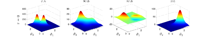
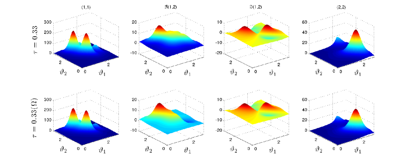
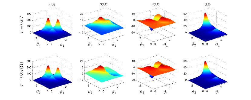
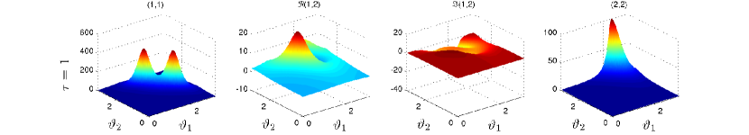
Figure 1: The path $\Phi_{\tau}(e^{j\bm{\vartheta}})$ between $\Phi_{0}(e^{j\bm{\vartheta}})$ and $\Phi_{1}(e^{j\bm{\vartheta}})$ for $\tau\in\{0,0.33,0.67,1\}$ using $\Omega$ defined in (38) – rows one, three, five and six – and $\Omega(e^{j\bm{\vartheta}})=I$ – rows one, two, four and six. The first and the last column show the entry of the spectral densities in position $(1,1)$ and $(2,2)$, respectively. The second and the third column show the real and the imaginary part of the entry of the spectral densities in position $(1,2)$.

VI The general case

The OTP’s analyzed before consider $\mathcal{P}$ as the set of Gaussian joint probability densities. This hypothesis, however, can be weakened. Notice that a Gaussian process is a particular elliptical process. More precisely, we can take $\mathcal{P}$ as the set of the joint probability densities such that $[\,\mathbf{x}^{T}\;\mathbf{y}^{T}\,]^{T}$ is an elliptical stationary process having zero mean and with joint power spectral density bounded and coercive. Accordingly, $\mathbf{x}$ and $\mathbf{y}$ are elliptical processes with zero mean. We conclude that the same reasoning and thus same results hold also in this case.

VII Conclusion

In this paper we have introduced the optimal transport problem between Gaussian aperiodic/periodic Gaussian random fields. The solution to these problems leads to a weighted Hellinger distance between multivariate and multidimensional power spectral densities. Such a distance can be characterized in terms of spectral factors. In the unidimensional case, the Hellinger distance can be defined in such a way to have the freedom in choosing one of these two spectral factors, see [8]; in particular, it is always possible to choose a rational spectral factor if the corresponding spectral density is rational. It is worth stressing that this last fact in the multidimensional case, however, is no longer true in general, [33, 34].

Finally, we have shown that the weighted Hellinger distance defines a geodesic, depending on the weight function, on the manifold of the multivariate and multidimensional spectral densities.

References

[1]
L. Kantorovich, “On the translocation of masses,” Doklady) Acad. Sci.
URSS (NS), vol. 37, pp. 199–201, 1942.
[2]
M. Knott and C. Smith, “On the optimal mapping of distributions,” Journal of Optimization Theory and Applications, vol. 43, no. 1, pp. 39–49,
1984.
[3]
T. Georgiou, J. Karlsson, and M. Takyar, “Metrics for power spectra: an
axiomatic approach,” IEEE Transactions on Signal Processing, vol. 57,
no. 3, pp. 859–867, 2008.
[4]
F. Elvander, A. Jakobsson, and J. Karlsson, “Interpolation and extrapolation
of Toeplitz matrices via optimal mass transport,” IEEE Transactions
on Signal Processing, vol. 66, no. 20, pp. 5285–5298, 2018.
[5]
L. Ning, T. Georgiou, and A. Tannenbaum, “On matrix-valued
Monge–Kantorovich optimal mass transport,” IEEE transactions on
automatic control, vol. 60, no. 2, pp. 373–382, 2015.
[6]
Y. Chen, T. Georgiou, L. Ning, and A. Tannenbaum, “Matricial Wasserstein-1
distance,” IEEE control systems letters, vol. 1, no. 1, pp. 14–19,
2017.
[7]
M. Zorzi, “Optimal transport between Gaussian stationary processes,” IEEE Transactions on Automatic Control, 2021.
[8]
A. Ferrante, M. Pavon, and F. Ramponi, “Hellinger versus Kullback-Leibler
multivariable spectrum approximation,” IEEE Trans. Autom. Control,
vol. 53, pp. 954–967, 2008.
[9]
F. Ramponi, A. Ferrante, and M. Pavon, “A globally convergent matricial
algorithm for multivariate spectral estimation,” IEEE Transactions on
Automatic Control, vol. 54, no. 10, pp. 2376–2388, 2009.
[10]
C. Byrnes, T. Georgiou, and A. Lindquist, “A new approach to spectral
estimation: A tunable high-resolution spectral estimator,” IEEE Trans.
Signal Processing, vol. 48, pp. 3189–3205, 2000.
[11]
T. Georgiou and A. Lindquist, “Kullback-Leibler approximation of spectral
density functions,” IEEE Transactions on Information Theory, vol. 49,
no. 11, pp. 2910–2917, 2003.
[12]
C. Byrnes, S. Gusev, and A. Lindquist, “A convex optimization approach to the
rational covariance extension problem,” SIAM J. Optim., vol. 37,
pp. 211–229, 1998.
[13]
J. Karlsson and T. Georgiou, “Uncertainty bounds for spectral estimation,”
IEEE Transactions on Automatic Control, vol. 58, no. 7, pp. 1659–1673,
2013.
[14]
M. Zorzi, “Rational approximations of spectral densities based on the Alpha
divergence,” Mathematics of Control, Signals, and Systems, vol. 26,
pp. 259–278, 2014.
[15]
A. Ferrante, C. Masiero, and M. Pavon, “Time and spectral domain relative
entropy: A new approach to multivariate spectral estimation,” IEEE
Trans. Autom. Control, vol. 57, pp. 2561–2575, 2012.
[16]
M. Zorzi, “Multivariate Spectral Estimation based on the concept of
Optimal Prediction,” IEEE Transactions on Automatic Control,
vol. 60, pp. 1647–1652, 2015.
[17]
M. Zorzi, “A new family of high-resolution multivariate spectral
estimators,” IEEE Transactions on Automatic Control, vol. 59,
pp. 892–904, 2014.
[18]
M. Zorzi, “An interpretation of the dual problem of the THREE-like
approaches,” Automatica, vol. 62, pp. 87–92, 2015.
[19]
M. Zorzi, “Empirical Bayesian learning in AR graphical models,” Automatica, vol. 109, p. 108516, 2019.
[20]
M. Zorzi, “Autoregressive identification of Kronecker graphical models,”
Automatica, vol. 119, p. 109053, 2020.
[21]
T. Georgiou, “Relative entropy and the multivariable multidimensional moment
problem,” IEEE Transactions on Information Theory, vol. 52, no. 3,
pp. 1052–1066, 2006.
[22]
A. Ringh, J. Karlsson, and A. Lindquist, “Multidimensional rational covariance
extension with applications to spectral estimation and image compression,”
SIAM Journal on Control and Optimization, vol. 54, no. 4,
pp. 1950–1982, 2016.
[23]
A. Ringh, J. Karlsson, and A. Lindquist, “Multidimensional rational covariance
extension with approximate covariance matching,” SIAM Journal on
Control and Optimization, vol. 56, no. 2, pp. 913–944, 2018.
[24]
B. Zhu, A. Ferrante, J. Karlsson, and M. Zorzi, “Fusion of sensors data in
automotive radar systems: A spectral estimation approach,” in 58th
Conference on Decision and Control (CDC 2019), pp. 5088–5093, 2019.
[25]
A. Ringh, J. Karlsson, and A. Lindquist, “The multidimensional circulant
rational covariance extension problem: Solutions and applications in image
compression,” in 54th Annual Conference on Decision and Control (CDC),
pp. 5320–5327, 2015.
[26]
B. Zhu, A. Ferrante, J. Karlsson, and M. Zorzi, “M2-spectral estimation:
A relative entropy approach,” Automatica, vol. 125, p. 109404, 2021.
[27]
B. Levy, R. Frezza, and A. Krener, “Modeling and estimation of discrete-time
Gaussian reciprocal processes,” IEEE Transactions on Automatic
Control, vol. 35, no. 9, pp. 1013–1023, 1990.
[28]
F. P. Carli, A. Ferrante, M. Pavon, and G. Picci, “A maximum entropy solution
of the covariance extension problem for reciprocal processes,” IEEE
Transactions on Automatic Control, vol. 56, no. 9, pp. 1999–2012, 2011.
[29]
A. G. Lindquist and G. Picci, “The circulant rational covariance extension
problem: The complete solution,” IEEE Transactions on Automatic
Control, vol. 58, no. 11, pp. 2848–2861, 2013.
[30]
A. Lindquist, C. Masiero, and G. Picci, “On the multivariate circulant
rational covariance extension problem,” in 52nd IEEE Conference on
Decision and Control, pp. 7155–7161, 2013.
[31]
D. Alpago, M. Zorzi, and A. Ferrante, “Identification of sparse
reciprocal graphical models,” IEEE Control Systems Letters, vol. 2,
no. 4, pp. 659–664, 2018.
[32]
L. Ning, X. Jiang, and T. Georgiou, “On the geometry of covariance
matrices,” IEEE Signal Processing Letters, vol. 20, no. 8,
pp. 787–790, 2013.
[33]
J. S. Geronimo and M. J. Lai, “Factorization of multivariate positive
Laurent polynomials,” Journal of Approximation Theory, vol. 139,
no. 1-2, pp. 327–345, 2006.
[34]
J. S. Geronimo and H. J. Woerdeman, “Positive extensions, Fejér-Riesz
factorization and autoregressive filters in two variables,” Annals of
Mathematics, pp. 839–906, 2004.