Failure extropy, dynamic failure extropy and their weighted versions

Abstract

Extropy was introduced as a dual complement of the Shannon entropy (see Lad et al. (2015)). In this investigation, we consider failure extropy and its dynamic version. Various basic properties of these measures are presented. It is shown that the dynamic failure extropy characterizes the distribution function uniquely. We also consider weighted versions of these measures. Several virtues of the weighted measures are explored. Finally, nonparametric estimators are introduced based on the empirical distribution function.

Keywords: Failure extropy, Dynamic failure extropy, weighted random variable, stochastic ordering, nonparametric estimators.

1 Introduction

Since its introduction, the Shannon entropy has been of primary interest in various applied fields of information theory. Recently, Lad et al. (2015) showed that a complementary dual function of the Shannon entropy exists. They called it extropy. Let $X$ be a nonnegative and absolutely continuous random variable with probability density function (pdf) $f$, cumulative distribution function (cdf) $F$ and survival function (sf) $\bar{F}=1-F.$ The extropy of $X$ is defined as (see Lad et al. (2015))

$$\mathcal{E}(X)=-\frac{1}{2}\int_{0}^{\infty}f^{2}(x)dx=-\frac{1}{2}E\left[f(X)\right].$$ (1.1)

From (1.1), it is clear that $\mathcal{E}(X)\in[-\infty,0).$ The concept of extropy is usually applied to score the forecasting distributions based on the total log scoring method. We refer to Gneiting and Raftery (2007), Furuichi and Mitroi (2012) and Vontobel (2012) for further applications of extropy. Qiu (2017) studied various properties of extropy for order statistics and record values. Similar to the residual entropy, Qiu and Jia (2018) proposed extropy for the residual random variable. They studied some properties including monotonicity and characterization of the residual extropy. Kamari and Buono (2020) introduced past extropy and obtained characterization result for the past extropy of the largest order statistic.

The Shannon differential entropy has some drawbacks. One of these is that it is defined for the distributions having density functions. For example, the definition of the Shannon differential entropy is not applicable for a mixture density comprised of a combination of Guassians and delta functions. Due to this, Rao et al. (2004) introduced cumulative residual entropy by substituting sf in place of the pdf in the definition of the differential entropy. Di Crescenzo and Longobardi (2009) proposed cumulative entropy based on the cdf and investigated various properties. Motivated by the way, the cumulative residual entropy was developed, Zografos and Nadarajah (2005) proposed the notion of the generalized survival entropy, which parallels the Renyi entropy. Inspired by the generalized survival entropy, Abbasnejad (2011) introduced generalized failure entropy and discussed various properties with some characterization results. Very recently, Sathar and Nair (2019) borrowed the notion of the survival entropy in order to propose survival extropy of a nonnegative and absolutely continuous random variable. It is given by

$$\mathcal{E}_{s}(X)=-\frac{1}{2}\int_{0}^{\infty}\bar{F}^{2}(x)dx.$$ (1.2)

This measure was constructed after replacing pdf by sf in (1.1). In this paper, we introduce failure extropy, dynamic failure extropy and their weighted versions. We point out that the failure extropy has been proposed similarly to the cumulative entropy (see Di Crescenzo and Longobardi (2009)) by substituting cdf in place of the pdf in (1.1). Before presenting main results, we recall some notions of various stochastic orders. These are useful in deriving some ordering results based on the proposed measures in the subsequent sections. Let $X$ and $Y$ be two nonnegative and absolutely continuous random variables with pdfs $f$ and $g$, cdfs $F$ and $G$, sfs $\bar{F}=1-F$ and $\bar{G}=1-G,$ respectively. The hazard and reversed hazard rates of $X$ and $Y$ are respectively denoted by $h_{X},h_{Y}$ and $r_{X},r_{Y}.$ Further, denote the right continuous inverses of $F$ and $G$ by $F^{-1}$ and $G^{-1}$, respectively.

Definition 1.1.

The random variable $X$ is said to be smaller than $Y$ in the

• usual stochastic order, denoted by $X\leq_{st}Y$, if $F(x)\geq G(x)$, for all $x$ in the set of real numbers;

• dispersive order, denoted by $X\leq_{disp}Y$, if $F^{-1}(\alpha)-F^{-1}(\beta)\leq G^{-1}(\alpha)-G^{-1}(\beta)$, for all $0<\beta\leq\alpha<1;$

• hazard rate order, denoted by $X\leq_{hr}Y$, if $h_{X}(x)\geq h_{Y}(x)$, for all $x>0$;

• reversed hazard rate order, denoted by $X\leq_{rh}Y$, if $r_{X}(x)\leq r_{Y}(x)$, for all $x>0$;

• likelihood ratio order, denoted by $X\leq_{lr}Y$, if $g(x)/f(x)$ is increasing with respect to $x>0.$

The terms increasing and decreasing are used in non-strict sense. The paper is organized as follows. In Section $2$, the failure extropy is proposed. We study various properties of it. In addition, the concept of the bivariate failure extropy is introduced. Section $3$ studies dynamic form of the failure extropy. Several properties similar to the failure extropy are investigated. It is shown that the dynamic failure extropy uniquely determines the distribution function. Further, a characterization for the power distribution is provided in Section $3$. Weighted versions of the failure extropy and the dynamic failure extropy are considered in Section $4.$ Properties related to the weighted measures are discussed. Nonparametric estimators of the measures are proposed in Section $5$. Real data sets are considered for the purpose of computation of the proposed estimators. Finally, concluding remarks are provided in Section $6.$

2 Failure extropy

In this section, we study some properties of the failure extropy. The definition of extropy, proposed here, is analogous to the definition of the cumulative entropy by Di Crescenzo and Longobardi (2009). Consider a nonnegative absolutely continuous random variable $X$ with support $S_{X},$ cdf $F$ and pdf $f$. The failure extropy of $X$, denoted by $\mathcal{E}_{f}(X)$ is defined as (see also Kundu (2020) and Nair and Sathar (2020))

$$\mathcal{E}_{f}(X)=-\frac{1}{2}\int_{0}^{\sup S_{X}}F^{2}(x)\mathrm{d}x.$$ (2.1)

Note that the above equation has been obtained after substituting the cdf of $X$ in place of the pdf in (1.1). Like extropy, the failure extropy given by (2.1) is always negative. Below, we obtain closed-form expressions for the failure extropy of various distributions.

Example 2.1.

• Let $X$ have uniform distribution in the interval $(0,b)$. Then, $\mathcal{E}_{f}(X)=-b/6.$

• Suppose $X$ has Type III extreme value distribution with cdf $F(x)=\exp\{\alpha(x-\beta)\},~{}x<\beta,~{}\alpha>0.$ Then, $\mathcal{E}_{f}(X)=-(e^{2\beta\alpha}-1)/(4\alpha e^{2\beta\alpha}).$

• Let us assume that $X$ follows power distribution with cdf $F(x)=x^{a},~{}0<x<1,~{}a>0.$ Then, $\mathcal{E}_{f}(X)=-1/(2(2a+1))$.

Remark 2.1.

If the support of the absolutely continuous random variable is unbounded, then the failure extropy is equal to $-\infty.$

In the following, we provide lower as well as upper bounds of the failure extropy when a random variable has bounded support. The lower bound can be achieved using $F^{2}(x)\leq F(x).$ On the other hand, the upper bound can be obtained utilizing Jensen’s inequality for integrals.

Proposition 2.1.

For a nonnegative and absolutely continuous random variable $X$ with support $[0,u]$ and cdf $F$, we have $(u<\infty)$

• $\mathcal{E}_{f}(X)\geq-\frac{1}{2}\int_{0}^{u}F(x)dx=-\frac{1}{2}[u-E(X)].$

• $\mathcal{E}_{f}(X)\leq-\frac{1}{2u}\left(\int_{0}^{u}F(x)dx\right)^{2}=-\frac{1}{2u}[u-E(X)]^{2}.$

Remark 2.2.

Let $X$ follow uniform distribution in the interval (0,u). Then, from the above proposition, lower and upper bounds of the extropy of uniform distribution can be obtained as $-u/4$ and $-u/8$, respectively. Clearly, $-u/4<\mathcal{E}_{f}(X)(=-u/6)<-u/8.$

Next, we take monotone transformations and examine its effect on the failure extropy.

Theorem 2.1.

Consider a nonnegative absolutely continuous random variable $X$ with cdf $F$. Take $\psi:S\rightarrow T$, a strictly monotone and differentiable function, where $S$ is the support of $X$ and $T$ is an interval, say $[u,v]$. Denote the failure extropy of $Y=\psi(X)$ by $\mathcal{E}_{f}(Y).$ Then,

$$\mathcal{E}_{f}(Y)=\begin{cases}-\frac{1}{2}\int_{\psi^{-1}(u)}^{\psi^{-1}(v)}\psi^{\prime}(x)F^{2}(x)dx,&if~{}\psi~{}\mbox{is strictly increasing;}\\ -\frac{1}{2}\int_{\psi^{-1}(v)}^{\psi^{-1}(u)}|\psi^{\prime}(x)|F^{2}(x)dx,&if~{}\psi~{}\mbox{is strictly decreasing.}\end{cases}$$

Proof.

We assume that $\psi$ is strictly increasing. The cdf of $Y$ is $G(y)=F(\psi^{-1}(y)).$ As a result, from the definition of the failure extropy, we have

$$\mathcal{E}_{f}(Y)=-\frac{1}{2}\int_{u}^{v}G^{2}(y)dy=-\frac{1}{2}\int_{u}^{v}F^{2}(\psi^{-1}(y))dy.$$ (2.2)

Now, utilizing the inverse transform $x=\psi^{-1}(y)$ in (2.2), the first part follows. The second part can be proved similarly and is omitted. This completes the proof. ∎

The following corollary is immediate from Theorem 2.1. It shows that the failure extropy is a shift-independent measure.

Corollary 2.1.

If $Y=aX+b$, where $a>0$ and $b\geq 0,$ then $\mathcal{E}_{f}(Y)=a\mathcal{E}_{f}(X).$

Let us now consider three nonnegative random variables $X,~{}X_{\tau}^{*}$ and $\tau X$, where $\tau>0.$ The cdf of $X_{\tau}^{*}$ is taken as $F^{*}(x)=[F(x)]^{\tau}.$ This is known as the proportional reversed hazard rate model. Now, we obtain inequality among the failure extropies of $X,~{}X_{\tau}^{*}$ and $\tau X$ (see also Nair and Sathar (2020)).

Proposition 2.2.

The inequalities $\mathcal{E}_{f}(X^{*}_{\tau})\leq\mathcal{E}_{f}(X)\leq\mathcal{E}_{f}(\tau X)$ hold when $\tau\in(0,1]$. The inequalities get reversed when $\tau\in[1,\infty).$

Proof.

The proof follows from Corollary 2.1 and the result $F^{2}(x)\leq(\geq)F^{2\tau}(x)$ when $0<\tau\leq 1~{}(\tau\geq 1)$. ∎

Remark 2.3.

Let $X_{1},\ldots,X_{n}$ be a random sample drawn from a population with cdf $F.$ Denote the largest order statistic of the sample by $X_{n:n}$. Further, it is known that the cdf of $X_{n:n}$ denoted by $F_{n:n}(x)$ is equal to $[F(x)]^{n},$ where $n$ is a positive integer. Thus, as an application of Proposition 2.2, we have $\mathcal{E}_{f}(nX_{1})\leq\mathcal{E}_{f}(X_{n:n})$.

The notions of partial orderings between the random variables have been introduced in the literature. These have useful applications in the theory of reliability and economics (see Shaked and Shanthikumar (2007)). Here, we propose a partial preorder, which helps to find out a better system in the sense of less uncertainty. Let $X$ and $Y$ be two nonnegative absolutely continuous random variables with cdfs $F$ and $G$, respectively. Next, let us define uncertainty order based on the failure extropy.

Definition 2.1.

A random variable $X$ is said to be smaller than $Y$ in the sense of the failure extropy, if $\mathcal{E}_{f}(X)\leq\mathcal{E}_{f}(Y).$ We denote $X\leq_{fe}Y$.

It is easy to see that the order defined above is a partial preorder, since it is reflexive, antisymmetric and transitive. There are many distributions for which the failure extropy order holds. For example, let us consider two random variables $X$ and $Y$ with respective cdfs $F(x)=x^{a_{1}}$ and $G(x)=x^{a_{2}}$, $0<x<1$. Further, let $0<a_{1}<a_{2}.$ Then, it can be clearly shown that $\mathcal{E}_{f}(X)\leq\mathcal{E}_{f}(Y)$, that is, $X\leq_{fe}Y$. Now, the question arises. Is there any relation between the usual stochastic order and the failure extropy order? The answer is yes. The following implication can be easily obtained from the definitions of the usual stochastic and failure extropy orders (see Nair and Sathar (2020))

$$X\leq_{st}Y\Rightarrow X\leq_{fe}Y.$$ (2.3)

Let $\{X_{1},\ldots,X_{m}\}$ be a collection of independent and identically distributed random observations. Denote the $l$th order statistic by $X_{l:m}$. It is not difficult to see that $X_{l:m}\leq_{st}X_{p:m}$, for all $1\leq l<p\leq m.$ For samples with possibly unequal sample sizes, we have $X_{m:m}\leq_{lr}X_{m+1:m+1}$ and $X_{1:m+1}\leq_{lr}X_{1:m}$ (see Shaked and Shanthikumar (2007)). Again, the likelihood ratio order implies the usual stochastic order. Thus, from (2.3), we have the following observations:

• $\mathcal{E}_{f}(X_{l:m})\leq\mathcal{E}_{f}(X_{p:m}),$ for all $1\leq l<p\leq m;$

• $\mathcal{E}_{f}(X_{m:m})\leq\mathcal{E}_{f}(X_{m+1:m+1});$

• $\mathcal{E}_{f}(X_{1:m+1})\leq\mathcal{E}_{f}(X_{1:m})$.

Further, it is well known that $X\leq_{disp}Y\Rightarrow X\leq_{st}Y.$ Thus, from (2.3), the extended implication chain is

$$X\leq_{disp}Y\Rightarrow X\leq_{st}Y\Rightarrow X\leq_{fe}Y.$$ (2.4)

It can be seen that the variance and differential entropy act additively when they are computed for the sum of two independent random variables. This property is not satisfied by the survival extropy. Below, we show that for two independent random variables, a lower bound of the failure extropy of the sum is the maximum of the individual failure extropies (also see Kundu (2020))

Proposition 2.3.

Consider two independent random variables $X$ and $Y$ having log-concave density functions. Then,

$$\mathcal{E}_{f}(X+Y)\geq\max\{\mathcal{E}_{f}(X),\mathcal{E}_{f}(Y)\}.$$

Proof.

Under the assumption that $X$ has log-concave density function and using Theorem $3.B.7$ of Shaked and Shanthikumar (2007), we obtain $X\leq_{disp}X+Y$. Thus, from (2.4), $\mathcal{E}_{f}(X)\leq\mathcal{E}_{f}(X+Y).$ Further, considering the case that $Y$ has log-concave density function, we get $\mathcal{E}_{f}(Y)\leq\mathcal{E}_{f}(X+Y).$ Combining these inequalities, we obtain the required result. ∎

Next, we derive conditions under which the failure extropy of two random variables can be ordered. It is known that a random variable $X$ has decreasing failure rate (DFR) if its failure rate function is decreasing. We have $X\leq_{disp}Y$ under the conditions that $X\leq_{hr}Y$ and $X$ or $Y$ is DFR. Thus, from (2.4), we have the following result.

Proposition 2.4.

If $X\leq_{hr}Y$ and $X$ or $Y$ is DFR, then $\mathcal{E}_{f}(X)\leq\mathcal{E}_{f}(Y).$

In the following proposition, we show that the failure extropy of $X$ can be expressed in terms of the expectations of $X$ and $Y$. Denote $R(x)=-\frac{1}{2}\int_{x}^{\infty}F(u)du.$

Proposition 2.5.

Consider two nonnegative and absolutely continuous random variables $X$ and $Y$ having unequal means and let $X\leq_{st}Y.$ If $R(x)<\infty$ and $E[R(Y)]<\infty$, then

$$\mathcal{E}_{f}(X)=E[R(Y)]+E[R^{\prime}(V)][E(Y)-E(X)],$$

where $V$ is nonnegative and absolutely continuous random variable with pdf

$$k(v)=\frac{\bar{G}(v)-\bar{F}(v)}{E(Y)-E(X)},~{}v>0$$

.

Proof.

The failure extropy can be expressed as $\mathcal{E}_{f}(X)=E(R(X)).$ Now, the rest of the proof follows from Di Crescenzo (1999). Thus, it is omitted. ∎

In this part of the section, we introduce failure extropy of bivariate random vector. Consider a bivariate random vector $(X,Y)$ with joint pdf $k$ and cdf $K$. The supports of $X$ and $Y$ are denoted by $S_{X}$ and $S_{Y}$, respectively. Further, assume that the marginal pdfs and cdfs of $X$ and $Y$ are denoted by $f,g$ and $F,G$, respectively. The bivariate failure extropy of $(X,Y)$ is defined as

$$\mathcal{E}_{f}(X,Y)=\frac{1}{4}\int_{0}^{\sup S_{X}}\int_{0}^{\sup S_{Y}}K^{2}(x,y)dxdy.$$ (2.5)

Let $X$ and $Y$ be independent, that is, $K(x,y)=F(x)G(y)$. Utilizing this in (2.5), we get

$$\mathcal{E}_{f}(X,Y)=\mathcal{E}_{f}(X)\mathcal{E}_{f}(Y).$$ (2.6)

This relation reveals that when $X$ and $Y$ are independent, the bivariate failure extropy has the additive property like the Shannon entropy. Now, we show that the bivariate failure extropy is not invariant under nonsingular transformations. Note that transformations play an important role to transform a distribution into another. So, it is always of interest to see the form of the bivariate failure extropy of the transformed random variables. Here we have studied the form of the bivariate failure extropy under the transformations $X_{i}\rightarrow\psi(X_{i})$, i=1,2.

Proposition 2.6.

Let $(Y_{1},Y_{2})$ be a nonnegative and absolutely continuous random vector. Further, let $Y_{i}=\psi(X_{i}),~{}i=1,2$ be one-to-one transformations such that $\psi(x_{i})$’s are differentiable. Then,

$$\mathcal{E}_{f}(Y_{1},Y_{2})=\frac{1}{4}\int_{0}^{\infty}\int_{0}^{\infty}K^{2}(x_{1},x_{2})|J|dx_{1}dx_{2},$$ (2.7)

where $J=\frac{\partial}{\partial x_{1}}\psi_{1}(x_{1})\frac{\partial}{\partial x_{2}}\psi_{2}(x_{2})$ is the Jacobian of the transformations.

Proof.

The proof is straightforward. Thus, it is omitted. ∎

Consider the conditional random variable $X|Y$ with cdf $K_{X|Y}(x|y)=\frac{K(x,y)}{G(y)}.$ Then, the conditional failure extropy is given by

$$\mathcal{E}_{f}(X|Y)=-\frac{1}{2}\int_{0}^{\infty}K^{2}_{X|Y}(x|y)dx.$$ (2.8)

Note that when $X$ and $Y$ are independent, then $K_{X|Y}(x|y)=F(x).$ Thus, clearly

$$\mathcal{E}_{f}(X|Y)=\mathcal{E}_{f}(X).$$

3 Dynamic failure extropy

In order to illustrate the effect of the age t on the uncertainty in random variables, dynamic information measures play a useful role in reliability. This section introduces dynamic version of the failure extropy. Suppose that a system is working. It is pre-planned that the system will be inspected at time $t>0$. At the inspection time, the system is down. Thus, uncertainty relies in the inactivity (past) time $(t-X|X<t).$ For the random variable $X$, the dynamic (past) failure extropy is defined as (see Kundu (2020) and Nair and Sathar (2020))

$$\mathcal{E}_{f}(X;t)=-\frac{1}{2}\int_{0}^{t}\left(\frac{F(x)}{F(t)}\right)^{2}dx,~{}t>0,~{}F(t)>0.$$ (3.1)

Under the condition that at time $t$, the system is down, $\mathcal{E}_{f}(X;t)$ quantifies the uncertainty about its past life. Clearly, $\mathcal{E}_{f}(X;0)=0$ and $\mathcal{E}_{f}(X;\infty)=\mathcal{E}_{f}(X)$. One can easily check that like the failure extropy, the dynamic failure extropy (DFE) takes negative values. The DFE of $X$ is equal to the failure extropy of the inactivity time. Now, we consider some distributions and obtain closed form expressions of the DFE.

Example 3.1.

• Let $X$ follow uniform distribution in the interval $(0,b)$. Thus, $F(x)=x/b$, $0<x<b$. Then, $\mathcal{E}_{f}(X;t)=-t/6$, for $0<t<b$.

• Let $X$ have type-III extreme value distribution with cdf $F(x)=\exp\{\alpha(x-\beta)\}$, $x<\beta$ and $\alpha>0$. Then, $\mathcal{E}_{f}(X;t)=-(\exp\{2\alpha t\}-1)/(4\alpha\exp\{2\alpha t\}),$ for $t<\beta.$

• Consider a Pareto random variable $X$ with cdf $F(x)=1-(b/x)^{a},~{}x>b>0,~{}a>0$. We obtain $\mathcal{E}_{f}(X;t)=-\frac{1}{2(1-(b/t)^{a})^{2}}[(t-b)+\frac{2b^{a}}{a-1}(\frac{1}{t^{a-1}}-\frac{1}{b^{a-1}})-\frac{b^{2a}}{2a-1}(\frac{1}{t^{2a-1}}-\frac{1}{b^{2a-1}})],$ for $a\neq 1,\frac{1}{2}$ and $t>b.$

We also consider exponential distribution with cdf $F(x)=1-e^{-\lambda x},~{}x>0,~{}\lambda>0$ to compute the DFE. This is given by

$$\mathcal{E}_{f}(X;t)=-\frac{1}{2(1-e^{-\lambda t})^{2}}\left[t+\frac{2e^{-\lambda t}}{\lambda}-\frac{e^{-2\lambda t}}{2\lambda}-\frac{2}{\lambda}+\frac{1}{2\lambda}\right].$$ (3.2)

For the purpose of visualization, we have depicted the DFE of exponential distribution for several values of the parameter $\lambda$ in Figure $1$.

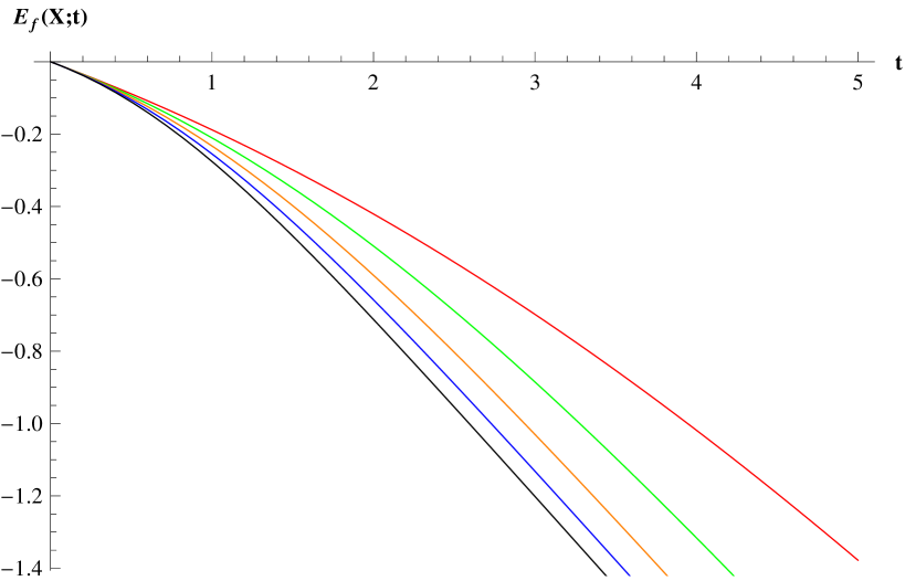
Figure 1: Plots of the dynamic failure extropy of the exponential distribution for various values of $\lambda.$ The values of $\lambda$ are taken as $0.5,~{}1,~{}1.5,~{}2$ and $2.5$ from above..

Similarly to Proposition 2.1, here, we obtain lower and upper bounds of the dynamic failure extropy. The proof is omitted.

Proposition 3.1.

Let $X$ be a nonnegative and absolutely continuous random variable with cdf $F.$ Further, denote the mean inactivity time of $X$ as $m_{I}(X;t)=E[t-X|X<t]=\int_{0}^{t}\frac{F(x)}{F(t)}dx.$ Then,

• $\mathcal{E}_{f}(X;t)\geq-\frac{1}{2F^{2}(t)}\int_{0}^{t}F(x)dx;$

• $\mathcal{E}_{f}(X;t)\leq-\frac{1}{2t}m_{I}^{2}(X;t).$

In the following theorem, we study the effect of monotone transformations on the DFE. The proof is similar to Theorem 2.1 and thus, it is omitted.

Theorem 3.1.

Let $X$ be a nonnegative absolutely continuous random variable with cdf $F$. Further, let $Y=\psi(X)$ be strictly monotone and differentiable. Denote the dynamic survival extropy of $Y$ by $\mathcal{E}_{f}(Y;t).$ Then,

$$\mathcal{E}_{f}(Y;t)=\begin{cases}-\frac{1}{2}\int_{\psi^{-1}(0)}^{\psi^{-1}(t)}\psi^{\prime}(x)\frac{F^{2}(x)}{F^{2}(\psi^{-1}(t))}dx,&if~{}\psi~{}\mbox{is strictly increasing;}\\ -\frac{1}{2}\int_{\psi^{-1}(t)}^{\psi^{-1}(0)}|\psi^{\prime}(x)|\frac{F^{2}(x)}{F^{2}(\psi^{-1}(t))}dx,&if~{}\psi~{}\mbox{is strictly decreasing.}\end{cases}$$

Below, we present the effect of the transformation $Y=\alpha X+\beta$, where $\alpha>0$ and $\beta\geq 0$ on the DFE. It immediately follows from Theorem 3.1.

Proposition 3.2.

If $Y=\alpha X+\beta$, where $\alpha>0$ and $\beta\geq 0$, then $\mathcal{E}_{f}(Y;t)=\alpha\mathcal{E}_{f}(X;\frac{t-\beta}{\alpha})$.

Sathar and Nair (2019) proposed ordering based on the dynamic survival extropy. Here, we consider ordering in terms of the DFE given by (3.1). One may refer to Kundu (2020) and Nair and Sathar (2020) for similar order.

Definition 3.1.

Let $X$ and $Y$ be two nonnegative and absolutely continuous random variables with cdfs $F$ and $G$, respectively. Then, $X$ is said to be samller than $Y$ in DFE, abbreviated by $X\leq_{dfe}Y$, if $\mathcal{E}_{f}(X;t)\leq\mathcal{E}_{f}(Y;t)$, for all $t>0.$

This definition of DFE ordering reveals that the uncertainty in $(X|X<t)$ about the predictability of the future time is smaller than that of $(Y|Y<t)$. Similar to the failure extropy order, the DFE order is also a partial order. Below, we obtain a connection between the reversed hazard rate ordering and the DFE ordering (also see Nair and Sathar (2020)).

Theorem 3.2.

Let $X$ and $Y$ be two nonnegative and absolutely continuous random variables with cdfs $F$ and $G$, respectively. Then,

$$X\leq_{rh}Y\Rightarrow X\leq_{dfe}Y.$$

Now, we consider an example, which is an application of Theorem 3.2.

Example 3.2.

Let $X_{1},\ldots,X_{n}$ be independent identical observations with reversed hazard rate $r$. Denote $X_{n:n}=\max\{X_{1},\ldots,X_{n}\}$ and its reversed hazard rate by $r_{n:n}(t)=nr(t).$ Then, $X_{1}\leq_{rh}X_{n:n}$. Thus, an application of Theorem 3.2 produces $\mathcal{E}_{f}(X_{1};t)\leq\mathcal{E}_{f}(X_{n:n};t).$

Remark 3.1.

Let $\xi$ be continuous and strictly increasing function. Then, from Nanda and Shaked (2001), we have

$$X\leq_{rh}Y\Rightarrow\xi(X)\leq_{rh}\xi(Y)\Rightarrow\mathcal{E}_{f}(\xi(X);t)\leq\mathcal{E}_{f}(\xi(Y);t)\Rightarrow\xi(X)\leq_{dfe}\xi(Y).$$ (3.3)

Basically, transformations are used to transform one probability density function into another. So, it is of interest to study if the uncertainty order (here $X\leq_{dfe}Y$) is preserved under some transformations. Next proposition provides sufficient conditions for preserving the ordering $X\leq_{dfe}Y$ under increasing (affine) transformations. Next result characterizes DFE ordering through increasing transformation.

Proposition 3.3.

Let $X$ and $Y$ be two nonnegative and absolutely continuous random variables such that $X\leq_{dfe}Y$. Let us take $Z_{1}=\alpha_{1}X+\beta_{1}$ and $Z_{2}=\alpha_{2}Y+\beta_{2}$ such that $0<\alpha_{1}\leq\alpha_{2}$ and $0<\beta_{1}\leq\beta_{2}.$ Then, $Z_{1}\leq_{dfe}Z_{2}$, provided $\mathcal{E}_{f}(X;t)$ is decreasing with respect to $t~{}(>\beta_{2})$.

Proof.

The proof follows under the assumptions made and Proposition 3.2. Thus, it is omitted. ∎

We propose a nonparametric class of distributions.

Definition 3.2.

A random variable $X$ with cdf $F$ belongs to the class of decreasing dynamic failure extropy (DDFE) if $\mathcal{E}_{f}(X;t)$ is decreasing with respect to $t.$

Clearly, uniform distribution belongs to this class. Next, we find conditions, under which the reversed hazard rate is decreasing. Note that Equation (3.1) can be alternatively expressed as

$$[F(t)]^{2}\mathcal{E}_{f}(X;t)=-\frac{1}{2}\int_{0}^{t}F^{2}(x)dx.$$ (3.4)

On differentiating (3.4) with respect to $t$, we obtain

$$\frac{d}{dt}\mathcal{E}_{f}(X;t)+2r(t)\mathcal{E}_{f}(X;t)+\frac{1}{2}=0,$$ (3.5)

where $r(t)=f(t)/F(t)$ is known as the reversed hazard rate of $X$. Further, differentiating (3.5) with respect to $t$, we get

$$\frac{d^{2}}{dt^{2}}\mathcal{E}_{f}(X;t)+2r^{\prime}(t)\mathcal{E}_{f}(X;t)+2r(t)\frac{d}{dt}\mathcal{E}_{f}(X;t)=0.$$ (3.6)

Thus, we have the following result.

Proposition 3.4.

Let $X$ be a nonnegative and absolutely continuous random variable. If $\mathcal{E}_{f}(X;t)$ is decreasing and concave, then $X$ has decreasing reversed hazard rate function.

The following proposition provides an upper bound of the reversed hazard rate function in terms of the DFE, when $X$ belongs to the DDFE class.

Proposition 3.5.

Let $X$ be an absolutely continuous and nonnegative random variable. Further, let $\mathcal{E}_{f}(X;t)$ be decreasing with respect to $t$. Then, $r(t)\leq-\frac{1}{4\mathcal{E}_{f}(X;t)}$.

Proof.

The proof follows from (3.5). ∎

It is always of interest to deal with the problem of characterizing probability distributions. The general characterization problem is to obtain conditions under which the DFE uniquely determines the distribution function. Next theorem shows that the DFE determines the distribution function uniquely. See Nair and Sathar (2020) for the proof.

Theorem 3.3.

Let $X$ have the cdf $F$ and reversed hazard rate function $r.$ Then, $\mathcal{E}_{f}(X;t)$ uniquely determines the cdf.

Let $(X_{1},X_{2})$ be the lifetimes of two units of a system. Assume that the first and second components are found failed at respective times $t_{1}$ and $t_{2}$. Then, the unceratinty associated with the past lifetimes of the system can be quantified by the two dimensional extension of the DFE. It is given by

$$\mathcal{E}_{f}(X_{1},X_{2};t_{1},t_{2})=\frac{1}{4}\int_{0}^{t_{1}}\int_{0}^{t_{2}}\left(\frac{K(x_{1},x_{2})}{K(t_{1},t_{2})}\right)^{2}dx_{1}dx_{2}.$$ (3.7)

Further, let $X_{1}$ and $X_{2}$ be independent. Therefore,

$$\mathcal{E}_{f}(X_{1},X_{2};t_{1},t_{2})=\mathcal{E}_{f}(X_{1};t_{1})\mathcal{E}_{f}(X_{2};t_{2}).$$ (3.8)

Similar to Proposition 2.6, it can be shown that the bivariate DFE is also not invariant under the nonsingular transformations $Y_{i}=\psi(X_{i}),~{}i=1,2$.

4 Weighted (dynamic) failure extropy

We now turn to the weighted versions of the failure extropy and DFE. In Balakrishnan et al. (2020), the authors studied the weighted versions of extropy and past extropy. First, let us discuss the weighted failure extropy. Note that the weighted distributions were introduced in the literature to get better fitted model of a dataset. Let $X$ be a nonnegative absolutely continuous random variable with cdf $F$ and pdf $f$. Then, the weighted (length-biased) random variable associated with the random variable $X$, denoted by $X_{w}$ has the pdf $f_{w}(t)=(w(t)f(t))/\mu_{w}$ and cdf $F_{w}(t)=(E[w(X)|X\leq t]F(t))/\mu_{w}$, where $w(x)~{}(\geq 0)$ is called weight function and $\mu_{w}=E(w(X))<\infty.$ Utilizing these, the failure extropy of $X_{w}$ is defined as

$$\mathcal{E}_{f}^{w}(X) = -\frac{1}{2}\int_{0}^{\infty}F^{2}_{w}(x)dx$$ (4.1)

$$= -\frac{1}{2\mu_{w}^{2}}\int_{0}^{\infty}\{E[w(X)|X\leq x]F(x)\}^{2}dx.$$

This is known as the weighted failure extropy (WFE). It takes negative values. Note that the WFE becomes the length-biased failure extropy when $w(x)=x.$ Let us denote the length-biased random variable by $X_{l}.$ Then, the pdf of $X_{l}$ is $f_{l}(t)=(tf(t))/\mu_{l}$ and cdf is $F_{l}(t)=(E[X|X\leq t]F(t))/\mu_{l},$ where $\mu_{l}=E(X).$ The failure extropy of $X_{l}$ is given by

$$\mathcal{E}_{f}^{l}(X) = -\frac{1}{2}\int_{0}^{\infty}F^{2}_{l}(x)dx$$ (4.2)

$$= -\frac{1}{2\mu_{l}^{2}}\int_{0}^{\infty}\{E[X|X\leq x]F(x)\}^{2}dx.$$

The following example illustrates the importance of the weighted (length-biased) failure extropy.

Example 4.1.

Consider two random variables $X$ and $Y$ with respective cdfs

$$F(x)=\begin{cases}0,&if~{}x\leq 2\\ \frac{x-2}{2},&if~{}2<x<4\\ 1,&if~{}x\geq 4\end{cases}$$ (4.3)

and

$$G(x)=\begin{cases}0,&if~{}x\leq 4\\ \frac{x-4}{2},&if~{}4<x<6\\ 1,&if~{}x\geq 6.\end{cases}$$ (4.4)

It can be computed that $\mathcal{E}_{f}(X)=\mathcal{E}_{f}(Y)=-\frac{1}{3},$ that is, the expected uncertainties contained in both distributions are the same. However, their associated uncertainties quantified via weighted (length-biased) failure entropy are not the same. These are obtained as $\mathcal{E}_{f}^{l}(X)\approx-0.2816$ and $\mathcal{E}_{f}^{l}(Y)\approx-0.813$.

The following proposition provides a lower bound of the weighted failure extropy based on the failure extropy. The similar statement also holds for the case of the length-biased failure extropy. The proof is straightforward and thus, it is omitted.

Proposition 4.1.

Let us assume that $E[w(X)|X\leq x]\leq E[w(X)].$ Then, $\mathcal{E}_{f}^{w}(X)\geq\mathcal{E}_{f}(X).$

In Section $2$, the inequalities of the failure extropies of the random variables $X_{\tau}^{*}$ and $X$ are obtained. Here, we try to obtain similar inequalities for the weighted version of the failure extropies of $X_{\tau}^{*}$ and $X$. We denote the weighted random variable associated with $X_{\tau}^{*}$ by $X_{w}^{*}.$ The cdf of $X_{w}^{*}$ is given by $F_{w}^{*}(x)=(E[w(X)|X\leq x]F^{\tau}(x))/\mu_{w}$. Thus, we have the following result. Its proof is similar to Proposition 2.2, and thus it is omitted.

Proposition 4.2.

Let $X$ be a nonnegative and absolutely continuous random variable with cdf $F$. Further, let $X_{\tau}^{*}$ be another random variable with cdf $F^{*}(x)=[F(x)]^{\tau},~{}\tau>0.$ Then, $\mathcal{E}_{f}^{w}(X_{\tau}^{*})\geq(\leq)\mathcal{E}_{f}^{w}(X)$ for $\tau>(<)1$.

Next, we introduce weighted form of the DFE. For the weighted random variable $X_{w}$, the DFE is defined as

$$\mathcal{E}_{f}^{w}(X;t) = -\frac{1}{2}\int_{0}^{t}\frac{F^{2}_{w}(x)}{F^{2}_{w}(t)}dx$$ (4.5)

$$= -\frac{1}{2}\int_{0}^{t}\frac{(E[w(X)|X\leq x]F(x))^{2}}{(E[w(X)|X\leq t]F(t))^{2}}dx.$$

This measure is known as the weighted DFE of the random variable $X$. Further, the length-biased DFE can be obtained from (4.5) by substituting $w(x)=x.$ It is given by

$$\mathcal{E}_{f}^{l}(X;t) = -\frac{1}{2}\int_{0}^{t}\frac{F^{2}_{l}(x)}{F^{2}_{l}(t)}dx$$ (4.6)

$$= -\frac{1}{2}\int_{0}^{t}\frac{(E[X|X\leq x]F(x))^{2}}{(E[X|X\leq t]F(t))^{2}}dx.$$

Differentiating (4.5) with respect to $t$, we obtain

$$\frac{d}{dt}\mathcal{E}_{f}^{w}(X;t)=-2r_{f}^{w}(t)\mathcal{E}_{f}^{w}(X;t)-\frac{1}{2},$$ (4.7)

where $r_{f}^{w}(t)=f_{w}(t)/F_{w}(t)$. Thus, we have the following proposition dealing with the bound of $\mathcal{E}_{f}^{w}(X;t).$

Proposition 4.3.

Let $\mathcal{E}_{f}^{w}(X;t)$ be decreasing with respect to $t$. Then, $\mathcal{E}_{f}^{w}(X;t)\geq-1/(4r_{f}^{w}(t)).$

Proof.

The proof of the proposition is immediate from (4.7). Thus, it is omitted. ∎

Similar to Proposition 3.4, we get the following result for the reversed hazard rate of the weighted random variable.

Proposition 4.4.

Let $\mathcal{E}_{f}^{w}(X;t)$ be decreasing and concave. Then, the weighted random variable $X_{w}$ has decreasing reversed hazard rate.

Proposition 4.5.

If $E[w(X)|X\leq x]\leq(\geq)E[w(X)|X\leq t]$ for $x\leq t$, then $\mathcal{E}_{f}^{w}(X;t)\geq(\leq)\mathcal{E}_{f}(X;t)$.

Proof.

The proof is straightforward and thus, it is omitted. ∎

The following corollary is immediate from the above proposition.

Corollary 4.1.

If $E[X|X\leq x]\leq(\geq)E[X|X\leq t]$ for $x\leq t$, then $\mathcal{E}_{f}^{l}(X;t)\geq(\leq)\mathcal{E}_{f}(X;t)$.

Now, we provide the effect of the scale transformation to the length-biased DFE.

Proposition 4.6.

Let $Y=aX$, where $a>0$. Then, $\mathcal{E}_{f}^{l}(Y;t)=a\mathcal{E}_{f}^{l}(X;t/a).$

Now, we define a nonparametric class based on the weighted DFE.

Definition 4.1.

A random variable $X$ with cdf $F$ is said to have decreasing weighted DFE, denoted by DWDFE if $\mathcal{E}_{f}^{w}(X;t)$ is decreasing with respect to $t>0.$

5 Estimation

In this section, we propose nonparametric estimators for the failure extropy, DFE and its weighted versions based on the empirical cumulative distribution function. Consider a simple random sample $(X_{1},\ldots,X_{n})$ of size $n$ from a population with cdf $F.$ The empirical distribution function of the sample is

$$\tilde{F}_{n}(x)=\frac{1}{n}\sum_{i=1}^{n}I(X_{i}\leq x),~{}~{}x\in\mathbb{R},$$ (5.1)

where $I$ is the indicator function. Denote the order statistics of $(X_{1},\ldots,X_{n})$ by $X_{(1)}\leq\ldots\leq X_{(i)}\leq\ldots\leq X_{(n)},$ where $X_{(i)}$ is the $i$th order statistic, $i=1,\ldots,n.$ Again,

$$\tilde{F}_{n}(x)=\displaystyle\left\{\begin{array}[]{ll}0,&\textrm{ $x<x_{(1)},$}\\ \frac{j}{n},&\textrm{$x_{(j)}\leq x<x_{(j+1)},~{}j=1,2,\ldots,n-1,$}\\ 1,&\textrm{$x\geq x_{(n)},$}\end{array}\right.$$

where $x_{(i)}$ is the realization of $X_{(i)}$. Thus, the empirical estimate of the failure extropy is

$$\mathcal{E}_{f}(\tilde{F}_{n}) = -\frac{1}{2}\int_{0}^{\sup S_{X}}\tilde{F}_{n}^{2}(x)dx$$ (5.3)

$$= -\frac{1}{2}\sum_{j=1}^{n-1}\int_{x_{(j)}}^{x_{(j+1)}}\tilde{F}_{n}^{2}(x)dx$$

$$= -\frac{1}{2}\sum_{j=1}^{n-1}\left(\frac{j}{n}\right)^{2}(x_{(j+1)}-x_{(j)}).$$

We consider two examples (see also Kayal (2016) and Di Crescenzo and Toomaj (2017)) which are dealing with exponential and uniform distributions.

Example 5.1.

Let $X_{1},\ldots,X_{n}$ be a random sample from exponential distribution with mean $1/\lambda,$ where $\lambda>0.$ Then, because of the independent sample spacings, $X_{(j+1)}-X_{(j)}$ follows exponential distribution with mean $1/(\lambda(n-j)).$ Thus, we have

$$E[\mathcal{E}_{f}(\tilde{F}_{n})]=-\frac{1}{2}\sum_{j=1}^{n-1}\left(\frac{j}{n}\right)^{2}\frac{1}{\lambda(n-j)}$$ (5.4)

and

$$Var[\mathcal{E}_{f}(\tilde{F}_{n})]=\frac{1}{4}\sum_{j=1}^{n-1}\left(\frac{j}{n}\right)^{4}\frac{1}{\lambda^{2}(n-j)^{2}}.$$ (5.5)

Example 5.2.

Consider a random sample $X_{1},\ldots,X_{n}$ from the uniform distribution in $(0,1)$. Then, $X_{(j+1)}-X_{(j)}$ follows beta distribution with parameters $1$ and $n$ with mean $E[X_{(j+1)}-X_{(j)}]=1/(n+1).$ Then.

$$E[\mathcal{E}_{f}(\tilde{F}_{n})]=-\frac{1}{2}\sum_{j=1}^{n-1}\left(\frac{j}{n}\right)^{2}\frac{1}{(n+1)}$$ (5.6)

and

$$Var[\mathcal{E}_{f}(\tilde{F}_{n})]=\frac{1}{4}\sum_{j=1}^{n-1}\left(\frac{j}{n}\right)^{4}\frac{n}{(n+1)^{2}(n+2)}.$$ (5.7)

Remark 5.1.

Clearly, from Example 5.2, we have

$$\lim_{n\rightarrow\infty}E[\mathcal{E}_{f}(\tilde{F}_{n})]=-1/6~{}~{}and~{}~{}\lim_{n\rightarrow\infty}Var[\mathcal{E}_{f}(\tilde{F}_{n})]=0.$$

This implies that the nonparametric estimator of the failure extropy is consistent when the random sample is taken from $U(0,1)$ distribution.

Now, for the case of the DFE, we assume that $x_{(1)}\leq\ldots\leq x_{(k)}\leq t\leq x_{(k+1)}\leq\ldots\leq x_{(n)},$ where $k=1,\ldots,n-1.$ Thus, the empirical DFE is given by

$$\mathcal{E}_{f}(\tilde{F}_{n};t) = -\frac{1}{2}\left[\sum_{j=1}^{k-1}\left(\frac{j}{k}\right)^{2}(x_{(j+1)}-x_{(j)})+(t-x_{(k)})\right].$$ (5.8)

Further, the nonparametric estimate of $\mathcal{E}_{f}^{w}(X)$ and $\mathcal{E}_{f}^{w}(X;t)$ are respectively given by

$$\mathcal{E}_{f}^{w}(\tilde{F}_{n}) = -\frac{1}{2}\left[\sum_{j=1}^{n-1}\left(\frac{j\sum_{i=1}^{j}w(x_{(i)})}{n\sum_{i=1}^{n}w(x_{(i)})}\right)^{2}(x_{(j+1)}-x_{(j)})\right],$$ (5.9)

$$\mathcal{E}_{f}^{w}(\tilde{F}_{n};t) = -\frac{1}{2}\left[\sum_{j=1}^{k-1}\left(\frac{j\sum_{i=1}^{j}w(x_{(i)})}{k\sum_{i=1}^{k}w(x_{(i)})}\right)^{2}(x_{(j+1)}-x_{(j)})+(t-x_{(k)})\right].$$ (5.10)

Next, we consider two real life data sets. The first consists of lifetimes (in days) of blood cancer patients (see Abu-Youssef (2002)) and the second contains spike times (in microseconds) of a neuron (see Kass et al. (2003)).

Example 5.3.

(i)  Lifetimes of blood cancer patients:-
$115,181,255,418,441,461,516,739,743,789,807,865,924,983,1024,1062,1063,1165,1191,\\ 1222,1222,1251,1277,1290,1357,1369,1408,1455,1478,1549,1578,1578,1599,1603,1605,\\ 1696,1735,1799,1815,1852.$

(ii)  Spike times observed in $8$ trials on a single neuron:-
$136.842,145.965,155.088,175.439,184.561,199.298,221.053,231.579,246.316,263.158,274.386,\\ 282.105,317.193,329.123,347.368,360.702,368.421,389.474,392.982,432.281,449.123,463.86,\\ 503.86,538.947,586.667,596.491,658.246,668.772,684.912.$

From the first set of data, we have $\mathcal{E}_{f}(\tilde{F}_{n})=-222.752$, $\mathcal{E}_{f}^{w}(\tilde{F}_{n})=-104.13$, $\mathcal{E}_{f}(\tilde{F}_{n};t=1000)=-128.069$ and $\mathcal{E}_{f}^{w}(\tilde{F}_{n};t=1000)=-55.237.$ Further, from the second dataset, we compute $\mathcal{E}_{f}(\tilde{F}_{n})=-113.135$, $\mathcal{E}_{f}^{w}(\tilde{F}_{n})=-50.9208$, $\mathcal{E}_{f}(\tilde{F}_{n};t=340)=-39.8138$ and $\mathcal{E}_{f}^{w}(\tilde{F}_{n};t=340)=-21.999.$

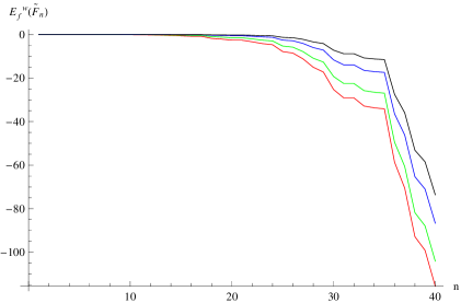
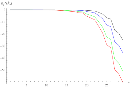
Figure 2: (a) Plot of the empirical estimator given by (5.9) for the the first dataset in Example 5.3 for various weight functions. The weight functions are taken as $w(x)=\sqrt{x},~{}x,~{}x^{2}$ and $x^{3}$ (from below to above). (b) Plot of the empirical estimator given by (5.9) for the the second dataset in Example 5.3 for various weight functions. The weight functions are taken as $w(x)=\sqrt{x},~{}x,~{}x^{2}$ and $x^{3}$ (from below to above).

6 Concluding remarks

Motivated by the concepts of the cumulative entropy and the failure entropy, in this paper, we have proposed failure extropy, dynamic failure extropy and their weighted versions. For failure extropy, we investigated various properties. Specifically, bounds, effect of monotone transformations and two dimensional version are studied. The uncertainty order based on the failure extropy has been introduced. Connection to other stochastic orders are also investigated. It has been shown that the usual stochastic order implies the failure extropy order. Since the failure extropy is not an useful tool to quantify uncertainty, which relies in a failed system, we also introduced a dynamic version of it. Similar properties have been discussed for this dynamic measure. A nonparametric class and some characterization results have been developed. Further, we have defined these measures for the weighted random variables. Various properties have been studied. Finally, empirical estimators of the proposed measures have been provided and computed numerically from two real life datasets.


Acknowledgements: The author would like to thank the Associate Editor and an anonymous reviewer for their positive remarks and useful comments. Suchandan Kayal gratefully acknowledges the partial financial support for this research work under a Grant MTR/2018/000350, SERB, India.

References

- (1)
- Abbasnejad (2011) Abbasnejad, M. (2011). Some characterization results based on dynamic survival and failure entropies, Communications for Statistical Applications and Methods. 18(6), 787–798.
- Abu-Youssef (2002) Abu-Youssef, S. (2002). A moment inequality for decreasing (increasing) mean residual life distributions with hypothesis testing application, Statistics & probability letters. 57(2), 171–177.
- Balakrishnan et al. (2020) Balakrishnan, N., Buono, F. and Longobardi, M. (2020). On weighted extropies, Communications in Statistics-Theory and Methods. pp. 1–31.
- Di Crescenzo (1999) Di Crescenzo, A. (1999). A probabilistic analogue of the mean value theorem and its applications to reliability theory, Journal of Applied Probability. 36(3), 706–719.
- Di Crescenzo and Longobardi (2009) Di Crescenzo, A. and Longobardi, M. (2009). On cumulative entropies, Journal of Statistical Planning and Inference. 139(12), 4072–4087.
- Di Crescenzo and Toomaj (2017) Di Crescenzo, A. and Toomaj, A. (2017). Further results on the generalized cumulative entropy, Kybernetika. 53(5), 959–982.
- Furuichi and Mitroi (2012) Furuichi, S. and Mitroi, F.-C. (2012). Mathematical inequalities for some divergences, Physica A: Statistical Mechanics and its Applications. 391(1-2), 388–400.
- Gneiting and Raftery (2007) Gneiting, T. and Raftery, A. E. (2007). Strictly proper scoring rules, prediction, and estimation, Journal of the American statistical Association. 102(477), 359–378.
- Kamari and Buono (2020) Kamari, O. and Buono, F. (2020). On extropy of past lifetime distribution, Ricerche di Matematica. pp. 1–11.
- Kass et al. (2003) Kass, R. E., Ventura, V. and Cai, C. (2003). Statistical smoothing of neuronal data, Network-Computation in Neural Systems. 14(1), 5–16.
- Kayal (2016) Kayal, S. (2016). On generalized cumulative entropies, Probability in the Engineering and Informational Sciences. 30(4), 640–662.
- Kundu (2020) Kundu, C. (2020). On cumulative residual (past) extropy of extreme order statistics, arXiv preprint arXiv:2004.12787. .
- Lad et al. (2015) Lad, F., Sanfilippo, G., Agro, G. et al. (2015). Extropy: complementary dual of entropy, Statistical Science. 30(1), 40–58.
- Nair and Sathar (2020) Nair, R. D. and Sathar, E. A. (2020). On dynamic failure extropy, Journal of the Indian Society for Probability and Statistics. 21(2), 287–313.
- Nanda and Shaked (2001) Nanda, A. K. and Shaked, M. (2001). The hazard rate and the reversed hazard rate orders, with applications to order statistics, Annals of the Institute of Statistical Mathematics. 53(4), 853–864.
- Qiu (2017) Qiu, G. (2017). The extropy of order statistics and record values, Statistics & Probability Letters. 120, 52–60.
- Qiu and Jia (2018) Qiu, G. and Jia, K. (2018). The residual extropy of order statistics, Statistics & Probability Letters. 133, 15–22.
- Rao et al. (2004) Rao, M., Chen, Y., Vemuri, B. C. and Wang, F. (2004). Cumulative residual entropy: a new measure of information, IEEE transactions on Information Theory. 50(6), 1220–1228.
- Sathar and Nair (2019) Sathar, E. and Nair, D. (2019). On dynamic survival extropy, Communications in Statistics-Theory and Methods. pp. 1–19.
- Shaked and Shanthikumar (2007) Shaked, M. and Shanthikumar, J. G. (2007). Stochastic orders, Springer Science & Business Media.
- Vontobel (2012) Vontobel, P. O. (2012). The bethe permanent of a nonnegative matrix, IEEE Transactions on Information Theory. 59(3), 1866–1901.
- Zografos and Nadarajah (2005) Zografos, K. and Nadarajah, S. (2005). Survival exponential entropies, IEEE transactions on information theory. 51(3), 1239–1246.