Low-Complexity Distance-Based Scheduling
for Multi-User XL-MIMO Systems

Abstract

We introduce Distance-Based Scheduling (DBS), a new technique for user selection in downlink multi-user communications with extra-large (XL) antenna arrays. DBS categorizes users according to their equivalent distance to the antenna array. Such categorization effectively accounts for inter-user interference while largely reducing the computational burden. Results show that (i) DBS achieves the same performance as the reference zero-forcing beamforming scheme with a lower complexity; (ii) a simplified version of DBS achieves a similar performance when realistic spherical-wavefront (SW) propagation features are considered; (iii) SW propagation brings additional degrees of freedom, which allows for increasing the number of served users.

I Introduction

The successful deployment of multi-user Multiple-Input Multiple-Output (MIMO) technology in the context of the 5G standard has been made possible by the massive MIMO concept [1]. As the commercial validation of massive MIMO is a key milestone in the roadmap of multi-user MIMO, the next steps move towards pushing the number of antennas and served users to a 10$\times$increase [2]. In this situation, the size of the extra-large (XL) antenna arrays becomes comparable to the user distances and the conventional far-field assumption no longer holds. Instead, non-stationary channel features need to be considered [3], which affect the scaling laws of the Signal-to-Noise Ratio (SNR) as the number of antennas grows [4].

Capacity-achieving schemes in multi-user MIMO based on dirty-paper coding (DPC) have a prohibitive complexity. Thus, the use of sub-optimal linear strategies based on Zero-Forcing (ZF) precoding to remove inter-user interference is usually preferred. ZF-beamforming (ZFBF) is known to have nearly as good performance as DPC, provided that a set of semi-orthogonal users are available for transmission [5]. However, since the computational complexity of linear precoders grows with the system dimensions, i.e., antennas and users [6], the problem of low-complexity user scheduling in XL-MIMO needs to be better examined. Besides, the interference behavior in XL-MIMO heavily depends on the user distances to the array elements, and interference can be incorrectly estimated when users are close to the antenna array [3].

The use of simple linear precoding techniques in the XL-MIMO regime was recently evaluated in [7], showing the impact of spatial non-stationarity on the downlink (DL) performance. The notion of visibility regions (VR) may partially alleviate the computational burden associated to ZF operation and Maximum Ratio Trasmission (MRT) through antenna selection [8], although the large array dimension still poses important challenges from a complexity viewpoint. Very recently, two low-complexity precoding schemes were proposed in [9] by a proper user grouping in the elevation domain. However, since both methods make use of a plane-wave (PW) approximation, their performance is degraded compared to the reference ZFBF for users closer to the Base Station (BS).

In this paper, we present two low-complexity techniques for DL user scheduling in XL-MIMO systems. Based on a novel definition of equivalent distance that accounts for the interference level, the user distance to the center of the array, and the number of antennas, we propose two schemes on which users are selected for transmission based on their equivalent distance to the BS; hence, we refer to these techniques as DBS. We show that DBS achieves the same performance as conventional ZFBF with a much lower complexity, while effectively capturing the spherical wavefront (SW) propagation experienced by users in the near-field region of the antenna array. We also see that a simplified-DBS scheme allows for an even lower complexity at the expense of a moderate performance degradation.

Notation: Throughout the article, lower-case bold letters denote vectors; the symbol $\sim$ reads as statistically distributed as; $\left(\cdot\right)^{\operatorname{T}}$ and $\left(\cdot\right)^{\operatorname{H}}$ denote the transpose and Hermitian transpose operations, respectively; ${\bf{1}}$ is the all-one vector; $\mathcal{N}_{\mathbb{C}}(0,\sigma^{2})$ is the zero-mean circularly symmetric Gaussian distribution with variance $\sigma^{2}$; $\|\cdot\|$ is the Euclidean norm; $\mathbb{C}^{M}$ is the $M$-dimensional complex vector space.

II System model

We consider an XL-MIMO setup where the BS deploys an extra-large antenna array with $M\gg 1$ elements, and communicates with $K$ single-antenna users. Without loss of generality, we assume a Uniform Linear Array (ULA) centered at the origin $\rm O$ and deployed along the ordinate axis. The position of the $k$-th user is then determined by the distance to the antenna array center, $r_{k}$, and the angle, $\theta_{k}$, formed by the line connecting user $k$ to $\rm O$ and the abscissa axis. Therefore, the array response vector ${\bf{a}}_{\rm k}\in\mathbb{C}^{M}$ reads as

$$\vspace{-1mm}{\bf{a}}_{\rm k}=[a_{1}(r_{k},\theta_{k}),a_{2}(r_{k},\theta_{k}),\ldots,a_{M}(r_{k},\theta_{k}))]^{\operatorname{T}},\vspace{-1mm}$$ (1)

where

$$\vspace{-1mm}a_{m}(r_{k},\theta_{k})=\tfrac{\sqrt{\beta_{0}}}{r_{k,m}}{\text{e}}^{-{\text{j}}\frac{2\pi}{\lambda}r_{k,m}},\vspace{-1mm}$$ (2)

is the $m$-th element of ${\bf{a}}_{\rm k}$, $\beta_{0}$ denotes the channel power at the reference distance $r_{\rm ref}=1$m, and $\lambda$ is the signal wavelength [4]. Finally, $r_{k,m}$ stands for the distance between the $k$-th user and the $m$-th element of the antenna array as

$$\vspace{-1mm}r_{k,m}=r_{k}\sqrt{1-2m{d}_{k}\sin\theta_{k}+{d}_{k}^{2}m^{2}},\,m\in\left[-\tfrac{M}{2},\tfrac{M}{2}\right],\vspace{-1mm}$$ (3)

with $d_{k}=\frac{d}{r_{k}}$, and $d$ is the separation between two consecutive antenna elements. As in [4, 10], we assume that the Line-of-Sight (LoS) component dominates the channel vector response.

Prior to transmission, the data symbols $s_{k}\sim\mathcal{N}_{\mathbb{C}}(0,1)$, $k=1,\ldots,K$ are precoded using the precoding vectors ${\bf{f}}_{\rm k}\in\mathbb{C}^{M}$, with $\|{\bf{f}}_{\rm k}\|=1$. The transmitted signal ${\bf{x}}_{\rm k}$ is then a linear combination of the precoded symbols, i.e., ${\bf{x}}_{\rm k}=\sum_{k}^{K}p_{k}{\bf{f}}_{\rm k}^{\operatorname{H}}s_{k}$, where $p_{k}$ are the power allocation scale factors such that $\sum_{k=1}^{K}p_{k}\leq P_{\text{TX}}$, with $P_{\text{TX}}$ the BS transmit power. For user $k$, the received signal $y_{k}$ is affected by the channel vector and the Additive White Gaussian Noise (AWGN) $n_{k}\sim\mathcal{N}_{\mathbb{C}}(0,\sigma^{2}_{w})$, as

$$\vspace{-1mm}y_{k}=p_{k}s_{k}{\bf{f}}_{\rm k}^{\operatorname{H}}{\bf{a}}_{\rm k}+\sum_{j\neq k}p_{j}s_{j}{\bf{f}}_{\rm j}^{\operatorname{H}}{\bf{a}}_{\rm k}+w_{k},\vspace{-1mm}$$ (4)

where the first term in (4) is the desired signal, and the second one represents the inter-user interference. Given the former expression, the achievable sum-rate is defined as [5]

$$\vspace{-1mm}R=\sum_{k=1}^{K}R_{k}=\sum_{k=1}^{K}\log_{2}\Bigg{(}1+\underbrace{\tfrac{|p_{k}{\bf{f}}_{\rm k}^{\operatorname{H}}{\bf{a}}_{\rm k}|^{2}}{\sigma^{2}_{w}+\sum_{j\neq k}|p_{j}{\bf{f}}_{\rm j}^{\operatorname{H}}{\bf{a}}_{\rm k}|^{2}}}_{\rm{SINR}_{k}}\Bigg{)},\vspace{-1mm}$$ (5)

where $\text{SINR}_{k}$ accounts for the $k$-th user Signal-to-Interference-plus-Noise Ratio (SINR). Our aim is to maximize the sum-rate in (5) subject to the power constraint, i.e.,

$$\vspace{-1mm}\operatorname*{argmax}_{\{{\bf{f}}_{\rm k},p_{k}\}_{k=1}^{K}}R\quad\text{s.t.}\quad\sum_{k=1}^{K}p_{k}\leq P_{\text{TX}}.\vspace{-.75mm}$$ (6)

We note from (5) that the achievable sum-rate is limited by the inter-user interference. However, the behavior of such interference severely changes with $r_{k,m}$ when near-field propagation effects are accounted for: e.g., the interference caused by users close to the BS is underestimated when assuming the PW model instead of (2). Conversely, as the spatial signature for each user depends on both their distances and their angles, when users $j$ and $k$ have similar angular values $\theta_{j}\approx\theta_{k}$ but different distances $r_{j}\neq r_{k}$, then the actual interference under the SW model is lower than that predicted by the PW assumption. With all the above considerations, a proper choice of the set of users $\mathcal{S}\subseteq\{1,\ldots,K\}$ served by the BS is crucial for the good functioning of the precoder and power allocation strategies. Hence, we split the problem in (6) into two sub-problems: (i) the selection of a user set $\mathcal{S}$ served by the BS according to the instantaneous channel conditions; and (ii) the precoder design and power allocation for the selected set $\mathcal{S}$.

III User scheduling in XL-MIMO

State-of-the-art user schedulers for massive MIMO setups employ the similarity between the channel vectors or the channel correlation matrices to perform user selection. These strategies become prohibitively complex in the XL-MIMO regime [11]. Besides, they often require a combinatorial search that is unfeasible for configurations with large $K$ and $M$ [6]. Greedy approximations [5, 12] reduce the number of combinations to check. This allows practical ZF schemes to achieve the capacity of DPC under the assumptions: (i) channel vectors with independent Gaussian entries and asymptotically large $K$, and (ii) PW model and sufficiently large $M$. Throughout this section, we propose a novel scheduling technique that largely alleviates the still large computational cost of conventional greedy schemes, while taking advantage of the specific features of XL-MIMO channels.

III-A Distance-Based Scheduling

We consider a greedy approach to joint scheduling and precoding inspired by superposition coding, where users are decoded according to their SNR levels. In our multi-user setup, we use the SINR definition in (5) so that users with larger SINRs are assigned higher priorities and, correspondingly, a larger allocation of the transmit power $P_{\text{TX}}$. In order to incorporate the interference caused by users enjoying higher priority levels, we base our scheduling policy on the concept of equivalent distance.

Let us consider the $n$-th iteration of the greedy procedure; the equivalent distance is defined as

$$r_{\text{eq},k}^{(n)}=r_{k}\Bigg{(}1-\frac{r_{k}^{2}}{M}\sum_{j\in\mathcal{S}^{(n)}}|{\bf{f}}^{{\operatorname{H}},(n)}_{\rm j}{\bf{a}}_{\rm k}|^{2}\Bigg{)}^{-1/2},$$ (7)

where $\mathcal{S}^{(n)}\subseteq\{1,\ldots,K\}$ is the sequence containing the $n$ served users, and ${\bf{f}}_{\rm j}^{(n)}$ is the precoder associated to user $j$, with $j\in\mathcal{S}^{(n)}$. In the initialization step, the equivalent distance $r_{\text{eq},k}^{(0)}$ is equal to the distance between the user and the BS, i.e., $r_{\text{eq},k}^{(0)}=r_{k}$. In (7), the equivalent distance is updated according to the level of interference caused by the scheduled users $\mathcal{S}^{(n)}$, the user distance to the BS $r_{k}$, and the number of antennas $M$. We see that for $\tfrac{r_{k}^{2}}{M}\ll 1$, the equivalent distance barely deviates from $r_{k}$ when including the interference caused by higher priority users. Conversely, when $\tfrac{r_{k}^{2}}{M}\gg 1$ inter-user interference strongly affects the computation of the equivalent distance. For a given $M$, these different behaviors are related to the distances between the users and the BS. The equivalent distance in (7) is used to assign higher priority levels to users close to the BS, as the impact of the inter-user interference is smaller than for users further away; therefore, we refer to this strategy as Distance-Based scheduling (DBS). In practice, the equivalent distance for user $k$ can be interpreted as an approximation to its $\text{SINR}_{k}$.

The set of precoders ${\bf{F}}(\mathcal{S}^{(n)})=[{\bf{f}}^{(n)}_{\rm k_{1}},\ldots,{\bf{f}}^{(n)}_{\rm k_{n}}]$, with $k_{1},\ldots,k_{n}\in\mathcal{S}^{(n)}$ is used to compute the equivalent distances (7), as the amount of interference depends on this choice. Considering the characteristics of the XL-MIMO setup with regard to the available spatial degrees of freedom and SNR regime, it is reasonable to apply ZF precoding at each iteration

$$\overline{{\bf{F}}}(\mathcal{S}^{(n)})=\left[{\bf{A}}(\mathcal{S}^{(n)})^{\operatorname{H}}\left({\bf{A}}(\mathcal{S}^{(n)}){\bf{A}}(\mathcal{S}^{(n)})^{\operatorname{H}}\right)^{-1}\right],$$ (8)

where ${\bf{A}}(\mathcal{S}^{(n)})=[{\bf{a}}^{(n)}_{\rm k_{1}},\ldots,{\bf{a}}^{(n)}_{\rm k_{n}}]^{\operatorname{T}}$ stacks the channel vectors corresponding to the sequence $\mathcal{S}^{(n)}$. To obtain the set of precoders ${\bf{F}}(\mathcal{S}^{(n)})$, we normalize the columns of $\overline{{\bf{F}}}(\mathcal{S}^{(n)})$. The equivalent channel gains $|{\bf{f}}_{\rm k}^{\operatorname{H}}{\bf{a}}_{\rm k}|^{2},\,k\in\mathcal{S}^{(n)}$ are then employed to compute the power allocation weights for the set of scheduled users ${\bf{p}}^{(n)}(\mathcal{S}^{(n)})\in\mathbb{R}^{n}$ using waterfilling.

Algorithm 1 Distance-Based Scheduling

1:  $n\leftarrow 0$, $\mathcal{S}^{(0)}\leftarrow\emptyset$, $\mathcal{K}\leftarrow\{1,\ldots,K\}$

2:  $r_{\text{eq},k}^{(0)}\leftarrow$ initialization

3:  repeat

4:     repeat

5:        $k\leftarrow\min_{i\in\mathcal{K}}r_{\text{eq},i}^{(n)}$

6:        $r_{\text{eq},k}^{(n)}\leftarrow$ update using (7)

7:        $q\leftarrow\min_{i\in\mathcal{K}}r_{\text{eq},i}^{(n)}$

8:     until $q=k$

9:     $n\leftarrow n+1$

10:     $\mathcal{S}^{(n)}\leftarrow\mathcal{S}^{(n-1)}\cup\{k\}$

11:     $\overline{{\bf{F}}}(\mathcal{S}^{(n)})\leftarrow$ Compute ZF precoders (8)

12:     ${\bf{F}}(\mathcal{S}^{(n)})\leftarrow$ Normalize $\overline{{\bf{F}}}(\mathcal{S}^{(n)})$ columns

13:     ${\bf{p}}^{(n)}(\mathcal{S}^{(n)})\leftarrow$ Power allocation using waterfilling

14:     $\mathcal{K}\leftarrow\mathcal{K}\setminus\{k\}$

15:  until $\mathcal{K}=\emptyset$ or stopping criterion

The proposed procedure for the DBS algorithm is summarized in Alg. 1: users start with their corresponding distances, and the algorithm seeks for the closest one to the BS. As new users are allocated, the equivalent distances are updated according to (7). If the user ordering does not change after the update, the closest user is selected as the candidate. Otherwise, the search continues with the following closest user. When the candidate user is selected, ZF precoders are computed according to the sequence $\mathcal{S}^{(n)}$, and then normalized to obtain the equivalent channel gains. Finally, these gains are used to decide the power distribution among users, ${\bf{p}}^{(n)}(\mathcal{S}^{(n)})$, with ${\bf{1}}^{\operatorname{T}}{\bf{p}}^{(n)}(\mathcal{S}^{(n)})=P_{\text{TX}}$. The algorithm ends after some stopping criterion is met like, for instance, a reduction on the achievable sum-rate or the maximum equivalent distance.

One interesting feature of DBS relies on the complexity reduction compared to the baseline greedy methods [5, 12], as we only evaluate the users within a certain distance range at each iteration of Alg. 1. This is especially noteworthy as the number of users $K$ grows and becomes comparable to $M$. Moreover, as we employ equivalent distances to determine the user ordering, most comparisons only involve scalars. Therefore, it is not only the number of comparisons that we reduce in DBS, but also the computational cost of making each of them. As we will later see, the relevant complexity reduction offered by DBS does not come at the price of a performance degradation compared to the ZFBF solutions [5].

III-B Simplified DBS

DBS algorithm allows to decrease the complexity associated to user selection; however, a moderately costly operation is necessary to update the equivalent distance in line 6 of the algorithm. We next evaluate an alternative to further reduce complexity at the expense of a certain performance loss.

From (7), it is clear that users with reduced $r_{k}$ are likely to be selected in the scheduling process, as the impact of the interference on the equivalent distance is proportional to $r_{k}^{2}$. Motivated by this observation, and noticing that an expensive step for the proposed DBS method is the distance update, we propose to use a naive approach that avoids this step. Therefore, the simplified DBS scheme, that we will refer to as DBS-s, will simply iterate using the distances $r_{k}$, regardless of the inter-user interference suffered by users with smaller priorities. Again, this approximation includes new users until a certain stopping criterion is met.

Note that, although the speed of this method is superior compared to regular DBS, the achievable performance of DBS-s strongly depends on the particular characteristics of the scenario. Consider, for example, a setup where users $1$ and $2$ are close to each other and satisfy $r_{1}<r_{2}\leq r_{k}$, $\forall k\in\{3,\ldots,K\}$. As the equivalent distance of user $2$ is not updated, the DBS-s algorithm would only serve user $1$. Hence, it is expected that the DBS-s scheme may incur in a performance loss, both in terms of served users and achievable rates. This will be assessed further in Section IV.

IV Numerical results

In this section, we provide the results of simulation experiments conducted to assess the advantages of the proposed scheduling methods. Table I shows the simulation parameter settings. The distance range considered is set to roughly twice the critical distance $r_{\text{cri}}=9Md$ in [4], which is the effective distance of the bound that separates the near-field and far-field regions. Since user distances within the coverage area are uniformly distributed, the proportion of users located in the near-field and far-field region is approximately $50\%$.

For benchmarking purposes, we compare the performance of the DBS and DBS-s methods with the classical linear precoding schemes considered in [7]. Specifically, we consider (i) the MRT precoder design followed by a waterfilling power allocation, and (ii) the greedy approach in [12] for ZFBF with successive user selection (SUS). The stopping criterion for the greedy approaches is a reduction on the achievable sum-rate. The SW propagation model in Section II is used, although reference results for the (incorrect) PW model associated to the far-field assumption are also included using dashed lines.

Table I: Simulation parameter settings.

Parameter	Value
Number of users	$K=1000$
Distance between antennas	$d=0.0628$ m
Transmit SNR ($\beta_{0}/\sigma^{2}_{w}$)	$\{0,5,10,15,20,25\}$ dB
Distance range	$[40,2r_{\text{cri}}-40]$ m
Angular range	$[-\frac{\pi}{4}\frac{\pi}{4}]$
Channel realizations	$1000$

Fig. 1 shows the achievable sum-rate $R$ as a function of the transmit SNR for all the schemes under evaluation. The first important observation is that the results obtained for the DBS and SUS schemes are equivalent regardless of the use of the SW or PW models, although for the latter model the achievable rate is slightly overestimated. This confirms that despite of using the equivalent distance as an approximation to the equivalent channel gains, there is no performance loss compared to the reference SUS. Remarkably, this will occur along all the ensuing investigated configurations. The performance of the MRT scheme notably degrades under SW propagation conditions. The opposite behavior is observed for the DBS-s scheme, for which the achievable rate is rather close to the reference schemes DBS/SUS. Hence, the DBS scheme can be seen as a simplified version of the SUS scheme but still offering, with lesser complexity, the best performance among the linear precoding schemes considered. This is confirmed by the execution times included in Table II which shows how DBS allows for a noticeable complexity reduction (around $80\%$) compared to SUS. For the DBS-s scheme, such reduction can even go well beyond $90\%$ at the expense of a minor performance degradation.

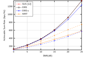
Figure 1: Achievable sum rate vs. SNR (dB) for $M=1000$ antennas. Parameter values are given in Table I. Solid/dashed lines correspond to the SW/PW models, respectively.

Table II: Execution time (ms)

Method/SNR(dB)	0	5	10	15	20	25
SUS [12]	3.65	5.35	7.46	10.18	13.25	18.14
DBS	0.35	0.57	0.94	1.50	2.33	3.72
DBS-s	0.16	0.30	0.50	0.76	1.15	1.70

Fig. 2 shows the number of served users as a function of the transmit SNR. As in the previous figure, the performance of SUS and DBS schemes is perfectly coincident. We see that a noticeable increase in served users is achieved when the SW propagation is accounted for, which is explained by the different interference behaviors exhibited by users closer to the antenna arrays. This provides more flexibility in the user selection, and allows to schedule a number of users larger than under the PW assumption. We also observe that while the performance of DBS-s seems poor under the PW assumption, it improves dramatically when the SW model is considered.

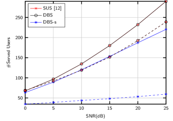
Figure 2: Number of served users vs. SNR (dB) for $M=1000$ antennas. Parameter values are given in Table I. Solid/dashed lines correspond to the SW/PW models, respectively.

Finally, the performance in terms of the number of antennas is evaluated in Fig. 3. As justified in Section III, the far-field approximation underestimates inter-user interference for users close to the BS, thus providing exceedingly optimistic performance results, especially when the number of antennas is small compared to the number of users. This observation is also supported by the results obtained with the simple MRT design. Conversely, the achievable sum-rates for the DBS-s scheme largely improves again under SW propagation conditions, so that including users close to the BS is key to obtain good performance results. This confirms the important role of the equivalent distance parameter accounting for the near-field propagation: for instance, the amount of inter-user interference between users with similar angular values is small if the distances are different.

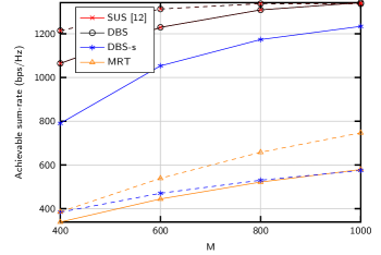
Figure 3: Achievable sum rate vs. number of antennas $M$ for SNR$=25$ dB. Parameter values are given in Table I. Solid/dashed lines correspond to the SW/PW models, respectively.

V Conclusion

The use of DBS schemes for user selection in DL XL-MIMO systems reduces the complexity of state-of-the-art methods. The performance of DBS is the same as that of the reference ZFBF approach. The complexity of DBS may be further reduced with a minor performance degradation under SW propagation. As a final remark, we pose that the optimality conditions for ZFBF may not hold in the XL-MIMO regime, as shown in the Appendix. This suggests that the development of capacity-approaching precoding techniques for XL-MIMO requires further investigation, although we conjecture that ZFBF (and hence, DBS) still can achieve the best performance among linear precoding schemes.

Appendix: On the optimality of ZFBF

Linear precoding achieves the performance of DPC under certain assumptions [5]. In XL-MIMO, however, this conclusion does not apply. In the following, we prove our statement constructively using a counter example.

Let us define a metric to characterize the power distribution among the transmit antenna elements. Such metric is given by the quotient between the normalized channel vector norm $\frac{1}{M}\|{\bf{a}}_{\rm k}\|^{2}=\frac{\beta_{0}\varphi}{Mr_{k}d\cos(\theta_{k})}$ from [4] and the maximum per-antenna-element power, $|a_{n}(r_{k},\theta_{k})|^{2}$, i.e.,

$$c(r_{k},\theta_{k}) =\tfrac{r_{k,n}^{2}\varphi}{Mr_{k}d\cos(\theta_{k})},$$ (9)

where $n\in\{-\frac{M}{2},\ldots,\frac{M}{2}\}$ is the index corresponding to the antenna array element closest to user $k$, and $\varphi\in[0,\pi]$ is

$$\varphi=\operatorname{atan}\left({\tfrac{Md-2r_{k}\sin(\theta_{k})}{2r_{k}\cos(\theta_{k})}}\right)+\operatorname{atan}\left(\tfrac{Md+2r_{k}\sin(\theta_{k})}{2r_{k}\cos(\theta_{k})}\right).$$

Next, consider users $k$ and $j$ and their associated distances and angles, i.e., $r_{k}$ and $r_{j}$, and $\theta_{k}$ and $\theta_{j}$, respectively. We now introduce the interference experienced by user $j$ if user $k$ employs the MRT precoder ${\bf{f}}_{\rm k}=\frac{1}{\|{\bf{a}}_{\rm k}\|}{\bf{a}}^{\operatorname{H}}_{\rm k}$. This leads to

$$|{\bf{f}}_{\rm k}^{\operatorname{H}}{\bf{a}}_{\rm j}|=\left|\sum_{m=-M/2}^{M/2}\tfrac{\beta_{0}}{\|{\bf{a}}_{\rm k}\|r_{m,i}r_{m,j}}{\text{e}}^{-{\text{j}}\frac{2\pi}{\lambda}(r_{m,j}-r_{m,i})}\right|,$$ (10)

with $r_{m,k}$ defined in (3). Without loss of generality, we assume that $r_{j}>r_{k}$, and consider $\theta_{k}=0$ for ease of exposition. Now, for $\frac{r_{k}^{2}}{M}\ll 1$, equation (9) shows that the transmit power concentrates over a reduced number of antennas $M^{\prime}\ll M$ close to the center of the array. Hence, for the significant antenna elements $m\in\{-M^{\prime}/2,\ldots,M^{\prime}/2\}$, the far-field assumption approximately holds and we have $a_{m}(r_{k},\theta_{k})\approx\tfrac{\sqrt{\beta_{0}}}{r_{k}}{\text{e}}^{-{\text{j}}\frac{2\pi}{\lambda}r_{k}}$ and $a_{m}(r_{j},\theta_{j})\approx\tfrac{\sqrt{\beta_{0}}}{r_{j}}{\text{e}}^{-{\text{j}}\frac{2\pi}{\lambda}(r_{j}-md\sin(\theta_{j}))}$. We rewrite (10) as

$$|{\bf{f}}_{\rm k}^{\operatorname{H}}{\bf{a}}_{\rm j}| \approx\tfrac{\beta_{0}}{\|{\bf{a}}_{\rm k}\|r_{k}r_{j}}\left|\sum_{m=-M^{\prime}/2}^{M^{\prime}/2}{\text{e}}^{-{\text{j}}\frac{2\pi}{\lambda}(r_{j}-md\sin(\theta_{j})-r_{k})}\right|$$

$$=\tfrac{\beta_{0}}{\|{\bf{a}}_{\rm k}\|r_{k}r_{j}}\left|\tfrac{\sin\left(\frac{\pi}{\lambda}dM^{\prime}\sin(\theta_{j})\right)}{\sin\left(\frac{\pi}{\lambda}d\sin(\theta_{j})\right)}\right|=i(\theta_{j}),$$ (11)

where $i(\theta_{j})$ accounts for the interference incident through angle $\theta_{j}$.

Next, we evaluate the probability of finding a set of semi-orthogonal users in the angular direction $\theta_{j}$. We introduce the interference threshold $\alpha$ and define the probability function $P\{i(\theta_{j})<\alpha\}$. To determine this probability, we define $\frac{M^{\prime}-1}{2}$ partitions $\mathcal{A}_{q}$ of the interval $[0,\frac{\pi}{2}]$, $\mathcal{A}_{q}=\left[l_{q,L},l_{q,U}\right]$, whose boundaries satisfy $i(l_{q,L})=i(l_{q,U})=0$. This condition is met for $l_{q,L}=\arcsin\left(\frac{\lambda q}{dM^{\prime}}\right)$, $l_{q,U}=\arcsin\left(\frac{\lambda(q+1)}{dM^{\prime}}\right)$, and $q\in\{0,(M^{\prime}-3)/2\}$. Based on these partitions, we determine $P\{i(\theta_{j})<\alpha\}$ as

$$P\{i(\theta_{j})<\alpha\}=2\sum_{q=0}^{\frac{M^{\prime}-1}{2}}P\{i(\theta_{j})<\alpha\,\cap\,\theta_{j}\in\mathcal{A}_{q}\}$$ (12)

$$\leq 2\sum_{q=0}^{\frac{M^{\prime}-1}{2}}P\left\{\left|\sin\left(\tfrac{\pi}{\lambda}dM^{\prime}\sin(\theta_{j})\right)\right|<\sin\left(\tfrac{\pi q}{M^{\prime}}\right)\alpha^{\prime}\,\cap\,\theta_{j}\in\mathcal{A}_{q}\right\}$$

where $\alpha^{\prime}=r_{k}r_{j}\alpha\|{\bf{a}}_{\rm k}\|\beta_{0}^{-1}$. The inequality results from bounding the denominator in (11) as $\sin\left(\frac{\pi}{\lambda}d\sin(\theta_{j})\right)\leq\sin\left(\frac{\pi q}{M^{\prime}}\right)$ for $\theta_{j}\in\mathcal{A}_{q}$; equality holds if $M^{\prime}\rightarrow\infty$. To compute (12), observe that there are two angles $\phi_{q,L},\phi_{q,U}\in\mathcal{A}_{q}$ fulfilling $\left|\sin\left(\frac{\pi}{\lambda}dM^{\prime}\sin(\phi_{q,L})\right)\right|=\left|\sin\left(\frac{\pi}{\lambda}dM^{\prime}\sin(\phi_{q,U})\right)\right|=\sin\left(\frac{\pi q}{M^{\prime}}\right)\alpha^{\prime}$. These angles follow the expressions

$$\phi_{q,L} =\arcsin\left(\tfrac{\lambda q}{M^{\prime}d}+\tfrac{\arcsin\left(\alpha^{\prime}\sin\left(\frac{\pi q}{M^{\prime}}\right)\right)}{\pi}\tfrac{\lambda}{M^{\prime}d}\right),$$ (13)

$$\phi_{q,U} =\arcsin\left(\tfrac{\lambda(q+1)}{M^{\prime}d}-\tfrac{\arcsin\left(\alpha^{\prime}\sin\left(\frac{\pi q}{M^{\prime}}\right)\right)}{\pi}\tfrac{\lambda}{M^{\prime}d}\right).$$

Using this result, we rewrite the probability in (12) as

$$\tfrac{P\{i(\theta_{j})<\alpha\}}{2} \leq\sum_{m=0}^{\frac{M^{\prime}-1}{2}}P\left\{\theta_{j}\in\left[l_{q,L},\phi_{q,L}\right]\right\}$$

$$+P\left\{\theta_{j}\in\left[\phi_{q,U},l_{q,U}\right]\right\}.$$ (14)

Note that $c(r_{k},0)$ in (9) satisfies $\lim_{M\rightarrow\infty}c(r_{k},0)=0$. Therefore, $M^{\prime}\approx 1$ in the asymptotic limit, and the right-hand side of (14) becomes $0$, regardless the chosen value of $\alpha$. It is therefore impossible to find a set of semi-orthogonal users. Furthermore, note that $\lim_{M\rightarrow\infty}c(r_{k},\theta_{k})=0$ also holds in the case $\theta_{k}\neq 0$. We note that $|\theta_{k}|>0$ leads to a smaller number of significant antennas $M^{\prime}$.

References

- [1] T. L. Marzetta, “Noncooperative Cellular Wireless with Unlimited Numbers of Base Station Antennas,” IEEE Trans. Wireless Commun., vol. 9, no. 11, pp. 3590–3600, 2010.
- [2] E. Björnson, L. Sanguinetti, H. Wymeersch, J. Hoydis, and T. L. Marzetta, “Massive MIMO is a reality—What is next?: Five promising research directions for antenna arrays,” Digit. Signal Process., vol. 94, pp. 3–20, 2019, special Issue on Source Localization in Massive MIMO.
- [3] E. D. Carvalho, A. Ali, A. Amiri, M. Angjelichinoski, and R. W. Heath, “Non-Stationarities in Extra-Large-Scale Massive MIMO,” IEEE Wireless Commun., vol. 27, no. 4, pp. 74–80, 2020.
- [4] H. Lu and Y. Zeng, “How Does Performance Scale with Antenna Number for Extremely Large-Scale MIMO?” 2020. [Online]. Available: https://arxiv.org/abs/2010.16232v1
- [5] Taesang Yoo and A. Goldsmith, “On the optimality of multiantenna broadcast scheduling using zero-forcing beamforming,” IEEE J. Sel. Areas Commun., vol. 24, no. 3, pp. 528–541, 2006.
- [6] A. Mueller, A. Kammoun, E. Björnson, and M. Debbah, “Linear precoding based on polynomial expansion: reducing complexity in massive MIMO,” EURASIP J. Wirel. Commun. Netw., vol. 2016, no. 1, p. 63, 2016.
- [7] A. Ali, E. D. Carvalho, and R. W. Heath, “Linear Receivers in Non-Stationary Massive MIMO Channels With Visibility Regions,” IEEE Wireless Commun. Lett., vol. 8, no. 3, pp. 885–888, 2019.
- [8] J. C. Marinello, T. Abrão, A. Amiri, E. de Carvalho, and P. Popovski, “Antenna Selection for Improving Energy Efficiency in XL-MIMO Systems,” IEEE Trans. Veh. Technol., vol. 69, no. 11, pp. 13 305–13 318, 2020.
- [9] L. N. Ribeiro, S. Schwarz, and M. Haardt, “Low-Complexity Zero-Forcing Precoding for XL-MIMO Transmissions,” arXiv preprint arXiv:2103.00971, 2021.
- [10] Z. Zhou, X. Gao, J. Fang, and Z. Chen, “Spherical Wave Channel and Analysis for Large Linear Array in LoS Conditions,” in 2015 IEEE Globecom Workshops (GC Wkshps), 2015, pp. 1–6.
- [11] A. Adhikary, J. Nam, J. Y. Ahn, and G. Caire, “Joint Spatial Division and Multiplexing: The Large-Scale Array Regime,” IEEE Trans. Inf. Theory, vol. 59, no. 10, pp. 6441–6463, October 2013.
- [12] C. Guthy, W. Utschick, and G. Dietl, “Low-Complexity Linear Zero-Forcing for the MIMO Broadcast Channel,” IEEE J. Sel. Top. Signal Process., vol. 3, no. 6, pp. 1106–1117, December 2009.