Existence, uniqueness, and approximation of a fictitious domain formulation for fluid-structure interactions

Abstract.

In this paper we describe a computational model for the simulation of fluid-structure interaction problems based on a fictitious domain approach. We summarize the results presented over the last years when our research evolved from the Finite Element Immersed Boundary Method (FE-IBM) to the actual Finite Element Distributed Lagrange Multiplier method (FE-DLM). We recall the well-posedness of our formulation at the continuous level in a simplified setting. We describe various time semi-discretizations that provide unconditionally stable schemes. Finally we report the stability analysis for the finite element space discretization where some improvements and generalizations of the previous results are obtained.

1. Introduction

In this paper we summarize in a unified setting some results of our research on the modeling and the approximation of fluid-structure interaction problems. Our aim is to describe the dynamics of a solid elastic body immersed in a Newtonian incompressible fluid. Here, we consider the so called zero-codimension case, that is the solid and the fluid are both two- or three-dimensional. From the mathematical point of view, the interaction is described by different partial differential equations in the regions occupied by the fluid and the solid, coupled with suitable transmission conditions along the interface between the two. It is well known that the numerical approximation of fluid-structure interaction problems is challenging for several reasons: first of all the numerical method must track the movement of the structure and the corresponding computational grids should allow the evaluation of quantities defined on moving domains. In this context, the use of a Lagrangian framework is more suited for the simulation of the structure deformation, while the approximation of the fluid velocity and pressure is better performed by an Eulerian approach.

Another crucial issue related to the approximation of fluid-structure interactions is how to deal with the coupling of the two underlying models: monolithic approaches perform the simultaneous computation of the fluid and structure unknowns, while partitioned schemes combine different solvers in the two subregions with an iterative procedure. In general monolithic schemes require implicit nonlinear solvers and a careful trade off between superior stability properties and more demanding computational load.

The research in this framework is very active and is based on a wide literature, ranging from boundary fitted approaches which, typically, use the so called Arbitrary Lagrangian Eulerian method [38, 28, 40, 29] to non fitted approaches which include, for instance, level set methods [21] Nitsche and XFEM methods [18, 1]. Our model belongs to the latter family originating from the Immersed Boundary Method (IBM) [45, 7] and evolved towards a fictitious domain approach in the spirit of [35, 34, 31, 33, 32, 52]. Obviously, no method is the optimal choice for all cases and, depending on the particular situation, it could be preferable to make use of different approaches; our formulation has the advantage to be unconditionally stable in time [6, 15] without the need of using fully implicit time schemes and, being based on non fitted meshes, can accommodate larger displacements. On the other hand, the coupling between fluid and structure models requires the evaluation of integrals that combine basis functions defined on different meshes. A solid mathematical analysis has been performed; we shall review some of the results in the following sections giving reference to the original papers when appropriate. Moreover, we extend the discretization of our model, allowing for more general choices of finite element spaces. We describe an incompressible solid immersed in an incompressible fluid; more general situation could be considered, involving compressible solids [13].

In Section 2 we recall the problem we are interested in, and introduce our fictitious domain formulation. Next, we analyze the continuous problem in Section 3 in a linearized setting, assuming that the motion of the solid is prescribed. Section 4 deals with the time discretization; the main result of this section is the unconditional stability of the evolution scheme. The space discretization is considered in Section 5 where a stability analysis is presented which leads to optimal convergence estimates for the steady state solution. Finally, Section 6 reports on several numerical tests that confirm the good behavior of our approach.

2. Model problem and fictitious domain formulation

The problem we want to address is easily explained in the following simplified setting. We consider a solid immersed in a fluid in two or three dimensions. At time $t$ the solid is located in the region $\Omega^{s}_{t}\subset\mathbb{R}^{d}$ ($d=2,3$) which is the image of a reference configuration $\mathcal{B}$ through a mapping $\mathbf{X}:\mathcal{B}\to\mathbb{R}^{d}$. The fluid occupies the region $\Omega^{f}_{t}\subset\mathbb{R}^{d}$ so that we are interested in a dynamic occurring in the union of $\Omega^{s}_{t}$ and $\Omega^{f}_{t}$. A typical assumption is that, denoting by $\Omega$ the interior of the union of the closures of $\Omega^{s}_{t}$ and $\Omega^{f}_{t}$, then $\Omega$ does not depend on $t$. This assumption is reasonable for several applications; in general $\Omega$ can be thought as a container where the dynamics takes place: for instance, the solid can be inside the fluid and far away from the exterior boundary of it, or the solid can touch one fixed part of the container. In this paper we deal with the first situation. We denote by $\Gamma_{t}$ the interface between fluid and solid, which can be defined as the interior of the intersection of $\overline{\Omega^{s}_{t}}$ and $\overline{\Omega^{f}_{t}}$.

The system is described by the fluid velocity $\mathbf{u}^{f}$ and pressure $p^{f}$, and by the solid position $\mathbf{X}$. The velocity and the pressure depend on time and on the space Eulerian variable $\mathbf{x}\in\Omega^{f}_{t}$, while the position $\mathbf{X}$ depends on time and on the Lagrangian variable $\mathbf{s}\in\mathcal{B}$. In the fixed domain $\Omega$ we are using the Eulerian framework and the corresponding variable $\mathbf{x}$. A point $\mathbf{x}$ of the domain $\Omega^{s}_{t}$ can be expressed at time $t$ in the Lagrangian setting as

$$\mathbf{x}=\mathbf{X}(\mathbf{s},t).$$

The kinematic condition is expressed by the following relationship between the material velocity $\mathbf{u}^{s}$ and $\mathbf{X}$:

$$\mathbf{u}^{s}(\mathbf{x},t)=\frac{\partial\mathbf{X}}{\partial t}(\mathbf{s},t),$$

where $\mathbf{x}=\mathbf{X}(\mathbf{s},t)$. The deformation gradient is given by

$$\mathbb{F}(\mathbf{s},t)=\frac{\partial\mathbf{X}}{\partial\mathbf{s}}(\mathbf{s},t).$$

We denote by $|\mathbb{F}|$ its determinant. We consider an incompressible solid, so that $|\mathbb{F}|$ is constant in time; in particular, in the case when $\mathcal{B}$ is the initial configuration $\Omega^{s}_{0}$ of $\Omega^{s}_{t}$, we have $|\mathbb{F}|=1$.

In the incompressible fluid the Navier–Stokes equations describe the dynamics as follows

(1) $$\rho_{f}\left(\frac{\partial\mathbf{u}^{f}}{\partial t}+\mathbf{u}^{f}\cdot\operatorname{\boldsymbol{\nabla}}\mathbf{u}^{f}\right)=\operatorname{\mathrm{div}}\boldsymbol{\sigma}^{f} \text{in }\Omega^{f}_{t}$$

$$\operatorname{\mathrm{div}}\mathbf{u}^{f}=0 \text{in }\Omega^{f}_{t},$$

where $\rho_{f}$ is the fluid density and $\boldsymbol{\sigma}^{f}$ is the Cauchy stress tensor that reads

$$\boldsymbol{\sigma}^{f}=-p^{f}{\mathbb{I}}+\nu_{f}\operatorname{\underline{\boldsymbol{\varepsilon}}}(\mathbf{u}^{f}),$$

$\nu_{f}>0$ being the viscosity of the fluid and $\operatorname{\underline{\boldsymbol{\varepsilon}}}$ the symmetric gradient.

We assume an incompressible viscoelastic material that can be described by a Cauchy stress tensor composed of two parts $\boldsymbol{\sigma}^{s}=\boldsymbol{\sigma}^{s}_{f}+\boldsymbol{\sigma}^{s}_{s}$: the first one is analogous to the fluid stress with the introduction of an artificial pressure $p^{s}$, which is the Lagrange multiplier associated with the incompressibility,

$$\boldsymbol{\sigma}^{s}_{f}=-p^{s}{\mathbb{I}}+\nu_{s}\operatorname{\underline{\boldsymbol{\varepsilon}}}(\mathbf{u}^{s}),$$

$\nu_{s}>0$ being the body viscosity; the second term is related to the Piola–Kirchhoff elasticity stress tensor $\mathbb{P}$ via the Piola transformation

$$\boldsymbol{\sigma}^{s}_{s}=|\mathbb{F}|^{-1}\mathbb{P}\mathbb{F}^{\top}.$$

The elastic part of the stress can be modeled using a potential energy density $W(\mathbb{F},\mathbf{s},t)$ so that

$$\mathbb{P}(\mathbb{F},\mathbf{s},t)=\frac{\partial W}{\partial\mathbb{F}}(\mathbb{F},\mathbf{s},t).$$

Taking all this into account, the equations describing the solid are

(2) $$\rho_{s}\frac{\partial^{2}\mathbf{X}}{\partial t^{2}}=\operatorname{\mathrm{div}}_{\mathbf{s}}(|\mathbb{F}|\boldsymbol{\sigma}_{f}^{s}\mathbb{F}^{-\top}+\mathbb{P}(\mathbb{F}))\ \text{in }\mathcal{B}$$

$$\operatorname{\mathrm{div}}\mathbf{u}^{s}=0 \text{in }\Omega^{s}_{t},$$

where $\rho_{s}$ is the solid density. The description of the model requires suitable transmission conditions enforcing the appropriate continuities of the velocity and of the Cauchy stress across the interface $\Gamma_{t}$ which can be stated as follows

(3) $$\mathbf{u}^{f}=\mathbf{u}^{s} \text{on }\partial\Omega^{s}_{t}$$

$$\boldsymbol{\sigma}^{f}\mathbf{n}_{f}=-(\boldsymbol{\sigma}^{s}_{f}+|\mathbb{F}|^{-1}\mathbb{P}\mathbb{F}^{\top})\mathbf{n}_{s} \text{on }\partial\Omega^{s}_{t},$$

where $\mathbf{n}_{f}$ and $\mathbf{n}_{s}$ stand for the outward unit normal vectors to $\Omega^{f}_{t}$ and $\Omega^{s}_{t}$, respectively. In conclusion, the system is described by (1), (2), (3), and the following initial and boundary conditions

(4) $$\mathbf{u}^{f}(0)=\mathbf{u}^{f}_{0} \text{in }\Omega^{f}_{0}$$

$$\mathbf{u}^{s}(0)=\mathbf{u}^{s}_{0} \text{in }\Omega^{s}_{0}$$

$$\mathbf{X}(0)=\mathbf{X}_{0} \text{in }\mathcal{B}$$

$$\mathbf{u}^{f}=0 \text{on }\partial\Omega.$$

Before describing our variational formulation we recall some standard notation that we are going to adopt [41]. Given a domain $D$, the space $\mathscr{D}(D)$ is the space of infinitely differentiable functions with compact support in $D$, $L^{2}(D)$ is the space of square integrable functions on $D$, the standard Sobolev spaces are denoted by $W^{s,p}(D)$, where $s\in\mathbb{R}$ refers to the differentiability and $p\in[1,+\infty]$ to the integrability exponent. As usual, when $p=2$ we use the notation $H^{s}(D)$. The corresponding norm is indicated by $\|\cdot\|_{s,D}$ and the scalar product in $L^{2}(D)$ by $(\cdot,\cdot)_{D}$; when no confusion arises we omit the indication of the domain $D$. In particular we will usually omit $\Omega$, while we will indicate explicitly when quantities are defined on the domain $\mathcal{B}$. $L^{2}_{0}(D)$ stands for the subspace of zero mean valued functions and $H^{1}_{0}(D)$ is the subset of functions in $H^{1}(D)$ with zero trace on $\partial D$. Given Banach spaces $X$ and $Y$, the notation $Y(0,T;X)$ contains space-time functions that for almost all $t\in 0,T$ are in $X$ and that are in $Y$ as functions from $(0,T)$ to $X$. Functional spaces of vector valued functions are indicated with boldface letters.

The main idea behind the fictitious domain approach that we are going to adopt, consists in extending the fluid variables inside the solid domain so that all involved quantities are defined in $\Omega$ (Eulerian variables) or $\mathcal{B}$ (Lagrangian variables). We started considering a fictitious domain model for a simplified interface problem [2, 14] which has been extended to fluid-structure interactions in [6].

We denote by $\mathbf{u}$ and $p$ the velocity and pressure in $\Omega$, with the understanding that their restrictions to the two subdomains $\Omega^{f}_{t}$ and $\Omega^{s}_{t}$ coincide with $\mathbf{u}^{f}$, $p^{f}$ and $\mathbf{u}^{s}$, $p^{s}$, respectively. With the aim of presenting a variational formulation of our problem, the condition $\mathbf{u}|_{\Omega^{s}_{t}}=\mathbf{u}^{s}$ will be enforced with the help of a bilinear form. Let $\boldsymbol{\Lambda}$ be a Hilbert space and $c:\boldsymbol{\Lambda}\times\mathbf{H}^{1}(\mathcal{B})\to\mathbb{R}$ a continuous bilinear form with the property

$$c(\boldsymbol{\mu},\mathbf{Y})=0\quad\forall\mu\in\boldsymbol{\Lambda}\quad\text{implies}\quad\mathbf{Y}=0.$$

The variational formulation is described by making use of the following notation.

$$\nu=\begin{cases}\nu_{f}&\text{in }\Omega^{f}_{t}\\ \nu_{s}&\text{in }\Omega^{s}_{t}\end{cases}$$

$$a(\mathbf{u},\mathbf{v})=\int_{\Omega}\nu\operatorname{\underline{\boldsymbol{\varepsilon}}}(\mathbf{u}):\operatorname{\underline{\boldsymbol{\varepsilon}}}(\mathbf{v})\,d\mathbf{x}$$

$$b(\mathbf{u},\mathbf{v},\mathbf{w})=\int_{\Omega}\frac{\rho_{f}}{2}\left((\mathbf{u}\cdot\operatorname{\boldsymbol{\nabla}}\mathbf{v})\cdot\mathbf{w}-(\mathbf{u}\cdot\operatorname{\boldsymbol{\nabla}}\mathbf{w})\cdot\mathbf{v}\right)\,d\mathbf{x}$$

$$\delta_{\rho}=\rho_{s}-\rho_{f}.$$

Problem 1 (Fictitious domain formulation).

Given $\mathbf{u}_{0}\in\mathbf{H}^{1}_{0}(\Omega)$, $\mathbf{X}_{0}\in\mathbf{W}^{1,\infty}(\mathcal{B})$, and $\mathbf{X}_{1}\in\mathbf{H}^{1}(\mathcal{B})$, find $\mathbf{u}(t)\in\mathbf{H}^{1}_{0}(\Omega)$, $p(t)\in L^{2}_{0}(\Omega)$, $\mathbf{X}(t)\in\mathbf{H}^{1}(\mathcal{B})$, and $\boldsymbol{\lambda}(t)\in\boldsymbol{\Lambda}$ such that, for almost every $t\in(0,T)$, it holds

(5) $$\rho_{f}\left(\frac{\partial\mathbf{u}}{\partial t}(t),\mathbf{v}\right)+b(\mathbf{u}(t),\mathbf{u}(t),\mathbf{v})+a(\mathbf{u}(t),\mathbf{v})$$

$$\qquad-(\operatorname{\mathrm{div}}\mathbf{v},p(t))+c\left(\boldsymbol{\lambda}(t),\mathbf{v}(\mathbf{X}(\cdot,t))\right)=0 \forall\mathbf{v}\in\mathbf{H}^{1}_{0}(\Omega)$$

$$(\operatorname{\mathrm{div}}\mathbf{u}(t),q)=0 \forall q\in L^{2}_{0}(\Omega)$$

$$\delta_{\rho}\left(\frac{\partial^{2}\mathbf{X}}{\partial t^{2}}(t),\mathbf{Y}\right)_{\mathcal{B}}+\left(\mathbb{P}(\mathbb{F}(t)),\operatorname{\boldsymbol{\nabla}}_{\mathbf{s}}\mathbf{Y}\right)_{\mathcal{B}}-c\left(\boldsymbol{\lambda}(t),\mathbf{Y}\right)=0 \forall\mathbf{Y}\in\mathbf{H}^{1}(\mathcal{B})$$

$$c\left(\boldsymbol{\mu},\mathbf{u}(\mathbf{X}(\cdot,t),t)-\frac{\partial\mathbf{X}}{\partial t}(t)\right)=0 \forall\boldsymbol{\mu}\in\boldsymbol{\Lambda}$$

$$\begin{aligned} &\mathbf{u}(0)=\mathbf{u}_{0}&&\text{in }\Omega\\ &\mathbf{X}(0)=\mathbf{X}_{0}&&\text{in }\mathcal{B}\\ &\frac{\partial\mathbf{X}}{\partial t}(0)=\mathbf{X}_{1}&&\text{in }\mathcal{B}.\end{aligned}$$

Remark 1.

The initial condition $\mathbf{X}_{1}$ in Problem 1 is related to $\mathbf{u}_{0}^{s}$ of 4 by the relation

$$\mathbf{X}_{1}=\mathbf{u}_{0}^{s}(\mathbf{X}_{0})\qquad\text{in $\mathcal{B}$}.$$

Various choices have been presented for the bilinear form $c$ responsible for the coupling of the Lagrangian and Eulerian frames.

In our setting two possible definitions of $c$ have been discussed in [6, 9]: a natural choice is to consider as $\boldsymbol{\Lambda}$ the dual space of $\mathbf{H}^{1}(\mathcal{B})$ so that $c$ can be taken as the duality pairing that certainly satisfies the required properties; a second equivalent choice stems from interpreting the duality pairing as the scalar product in $\mathbf{H}^{1}(\mathcal{B})$ by the Riesz representation theorem so that $\boldsymbol{\Lambda}=\mathbf{H}^{1}(\mathcal{B})$. More in detail, we have the following definitions

1. $\boldsymbol{\Lambda}_{1}=\mathbf{H}^{1}(\mathcal{B})^{\prime}$ and $c_{1}:\boldsymbol{\Lambda}_{1}\times\mathbf{H}^{1}(\mathcal{B})\to\mathbb{R}$ with

   (6) $$c_{1}(\boldsymbol{\mu},\mathbf{Y})={}_{\boldsymbol{\Lambda}_{1}}\langle\boldsymbol{\mu},\mathbf{Y}\rangle_{\mathbf{H}^{1}(\mathcal{B})}$$

2. $\boldsymbol{\Lambda}_{2}=\mathbf{H}^{1}(\mathcal{B})$ and $c_{2}:\boldsymbol{\Lambda}_{2}\times\mathbf{H}^{1}(\mathcal{B})\to\mathbb{R}$ with

   (7) $$c_{2}(\boldsymbol{\mu},\mathbf{Y})=(\boldsymbol{\mu},\mathbf{Y})_{\mathcal{B}}+(\operatorname{\boldsymbol{\nabla}}_{\mathbf{s}}\boldsymbol{\mu},\operatorname{\boldsymbol{\nabla}}_{\mathbf{s}}\mathbf{Y})_{\mathcal{B}}.$$

While the two definitions are equivalent for the continuous problem, they give rise to different discretizations. In the sequel we are going to use the generic notation $\boldsymbol{\Lambda}$ and $c$, while indicating explicitly one of the two cases when needed.

An analogous formulation, which is outside the topics of the present work, can also be used in the case of codimension one structures. We refer the interested reader to [6, 9].

We end this section by stating a stability result for the continuous problem which was proved in [6].

Proposition 1.

Let $\mathbf{u}(t)\in\mathbf{H}^{1}_{0}(\Omega)$ and $\mathbf{X}(t)\in\mathbf{H}^{1}(\mathcal{B})$ be solutions of Problem 1. Assume that $\partial\mathbf{X}(t)/\partial t\in\mathbf{L}^{2}(\mathcal{B})$ and consider the elastic potential energy of the body given by

$$E\left(\mathbf{X}(t)\right)=\int_{\mathcal{B}}W(\mathbb{F}(\mathbf{s},t))\,d\mathbf{s}.$$

Then the following conservation property is satisfied for almost every $t\in(0,T)$

$$\frac{\rho_{f}}{2}\frac{d}{dt}||\mathbf{u}(t)||^{2}_{{0,\Omega}}+||\nu^{1/2}\operatorname{\underline{\boldsymbol{\varepsilon}}}(\mathbf{u}(t))||^{2}_{{0,\Omega}}+\frac{\delta_{\rho}}{2}\frac{d}{dt}\left\|\frac{\partial\mathbf{X}}{\partial t}(t)\right\|^{2}_{{0,\mathcal{B}}}+\frac{d}{dt}E(\mathbf{X}(t))=0.$$

3. Existence and uniqueness of the linearized problem

Not many results are available in the literature about existence and uniqueness of the solution to fluid-structure interaction problems. This is not surprising since the coupling between fluids and solids gives rise in general to highly non linear problems. In the case when a fluid is containing rigid solids or elastic bodies described by a finite number of modes, existence and uniqueness of weak solutions have been studied for instance in [22, 25, 26, 27, 30, 36, 37, 39, 47, 48, 49]; when a fluid is enclosed in a solid membrane then the existence and uniqueness of weak solutions have been discussed in [3, 20, 42, 43]. Moreover, local-in-time existence and uniqueness of strong solutions for an elastic structure immersed in a fluid are proved in [23, 24, 46, 16, 17].

In this section we describe the analysis performed in [11] about the existence and the uniqueness of a linearization of Problem 1 in the case when $\boldsymbol{\Lambda}=\mathbf{H}^{1}(\mathcal{B})$ and the bilinear form $c$ is equal to the scalar product in $\mathbf{H}^{1}(\mathcal{B})$. This is a first step towards the analysis of the full problem which could make use of some fixed point strategy.

We consider a given function $\overline{\mathbf{X}}$ that describes the motion of the solid. We assume that $\overline{\mathbf{X}}$ belongs to $C^{1}([0,T];\mathbf{W}^{1,\infty}(\mathcal{B}))$, is invertible with Lipschitz inverse, and coincides with the identity at time $t=0$, that is $\overline{\mathbf{X}}(\mathbf{s},0)=\mathbf{s}$. Moreover, we assume that the motion of the solid is compatible with the incompressibility constraint, that is $\det(\operatorname{\boldsymbol{\nabla}}_{\mathbf{s}}\overline{\mathbf{X}}(t))=1$ for all $t$.

We choose a linear model for the elasticity, namely $\mathbb{P}(\mathbb{F})=\kappa\mathbb{F}$; moreover, we introduce a new variable $\mathbf{w}(t)$ equal to the velocity of the solid $\partial\mathbf{X}(t)/\partial t$, so that, after neglecting the convective term in the Navier–Stokes equation, we are led to the following problem.

Problem 2 (Linearized formulation).

Let us assume that $\overline{\mathbf{X}}\in C^{1}([0,T];\mathbf{W}^{1,\infty}(\mathcal{B}))$ satisfies the hypotheses described above. Given $\mathbf{u}_{0}\in\mathbf{H}^{1}_{0}(\Omega)$, $\mathbf{X}_{0}\in\mathbf{W}^{1,\infty}(\mathcal{B})$, and $\mathbf{X}_{1}\in\mathbf{H}^{1}(\mathcal{B})$, find $\mathbf{u}(t)\in\mathbf{H}^{1}_{0}(\Omega)$, $p(t)\in L^{2}_{0}(\Omega)$, $\mathbf{X}(t)\in\mathbf{H}^{1}(\mathcal{B})$, $\mathbf{w}\in\mathbf{H}^{1}(\mathcal{B})$, and $\boldsymbol{\lambda}(t)\in\mathbf{H}^{1}(\mathcal{B})$ such that, for almost every $t\in(0,T)$, it holds

(8) $$\rho_{f}\left(\frac{\partial\mathbf{u}}{\partial t}(t),\mathbf{v}\right)+a(\mathbf{u}(t),\mathbf{v})-(\operatorname{\mathrm{div}}\mathbf{v},p(t))$$

$$\qquad\qquad\qquad\qquad\qquad+c(\boldsymbol{\lambda}(t),\mathbf{v}(\overline{\mathbf{X}}(\cdot,t)))=0 \forall\mathbf{v}\in\mathbf{H}^{1}_{0}(\Omega)$$

$$(\operatorname{\mathrm{div}}\mathbf{u}(t),q)=0 \forall q\in L^{2}_{0}(\Omega)$$

$$\delta_{\rho}\left(\frac{\partial\mathbf{w}}{\partial t}(t),\mathbf{Y}\right)_{\mathcal{B}}+\kappa(\operatorname{\boldsymbol{\nabla}}_{\mathbf{s}}\mathbf{X}(t),\operatorname{\boldsymbol{\nabla}}_{\mathbf{s}}\mathbf{Y})_{\mathcal{B}}-c(\boldsymbol{\lambda}(t),\mathbf{Y})=0 \forall\mathbf{Y}\in\mathbf{H}^{1}(\mathcal{B})$$

$$\left(\frac{\partial\mathbf{X}}{\partial t}(t),\mathbf{y}\right)_{\mathcal{B}}=(\mathbf{w}(t),\mathbf{y})_{\mathcal{B}} \forall\mathbf{y}\in\mathbf{L}^{2}(\mathcal{B})$$

$$c\left(\boldsymbol{\mu},\mathbf{u}(\overline{\mathbf{X}}(\cdot,t),t)-\mathbf{w}(t)\right)=0 \forall\boldsymbol{\mu}\in\mathbf{H}^{1}(\mathcal{B})$$

$$\begin{aligned} &\mathbf{u}(0)=\mathbf{u}_{0}&&\text{in }\Omega\\ &\mathbf{X}(0)=\mathbf{X}_{0}&&\text{in }\mathcal{B}\\ &\mathbf{w}(0)=\mathbf{X}_{1}&&\text{in }\mathcal{B}.\end{aligned}$$

The following existence and uniqueness result was proved in [11].

Theorem 2.

Under the assumptions reported above, there exists a unique solution to Problem 8 that satisfies the following regularity

$$\mathbf{u}\in\mathbf{L}^{\infty}(0,T;\mathbf{H}_{0})\cap\mathbf{L}^{2}(0,T;\mathbf{V}_{0})$$

$$p\in L^{2}(0,T;L^{2}_{0}(\Omega))$$

$$\mathbf{X}\in\mathbf{L}^{\infty}(0,T;\mathbf{H}^{1}(\mathcal{B}))$$

$$\mathbf{w}\in\mathbf{L}^{\infty}(0,T;\mathbf{L}(\mathcal{B}))\cap\mathbf{L}^{2}(0,T;\mathbf{H}^{1}(\mathcal{B}))$$

$$\boldsymbol{\lambda}\in\mathbf{L}^{2}(0,T;\mathbf{H}^{1}(\mathcal{B})),$$

where

$$\mathscr{V}_{0}=\{\mathbf{v}\in\mathscr{D}(\Omega)^{d}:\operatorname{\mathrm{div}}\mathbf{v}=0\}$$

$$\mathbf{H}_{0}=\text{ the closure of }\mathscr{V}_{0}\text{ in }L^{2}_{0}(\Omega)$$

$$\mathbf{V}_{0}=\text{ the closure of }\mathscr{V}_{0}\text{ in }\mathbf{H}^{1}_{0}(\Omega).$$

The proof of this result is obtained by considering first a reduced problem where the unknowns $p$ and $\boldsymbol{\lambda}$ are eliminated since the velocity is sought in the kernel of the divergence operator $\mathbf{V}_{0}$ and the pair $(\mathbf{u}(t),\mathbf{w}(t))$ is required to satisfy the constraint

(9) $$c\left(\boldsymbol{\mu},\mathbf{u}(\overline{\mathbf{X}}(\cdot,t),t)-\mathbf{w}(t)\right)=0\quad\forall\boldsymbol{\mu}\in\mathbf{H}^{1}(\mathcal{B}).$$

In this setting, the proof follows a suitable modification of the Galerkin arguments used in [50] for the analysis of Navier–Stokes equations.

Finally, the Lagrange multiplier and the pressure are recovered by using Lax–Milgram lemma and the Banach closed range theorem.

4. Time advancing schemes

We begin in this section the study of the numerical approximation of Problem 1, starting from the time discretization.

Let us introduce a time discretization parameter $\Delta t$, and let us denote by $t_{n}$, $n=0,\dots,N$ the corresponding nodes; the following system is obtained by the application of the backward Euler scheme.

Problem 3 (Backward Euler scheme).

Given $\mathbf{u}_{0}\in\mathbf{H}^{1}_{0}(\Omega)$, $\mathbf{X}_{0}\in\mathbf{W}^{1,\infty}(\mathcal{B})$, and $\mathbf{X}_{1}\in\mathbf{H}^{1}(\mathcal{B})$, for all $n=1,\dots,N$ find $\mathbf{u}^{n}\in\mathbf{H}^{1}_{0}(\Omega)$, $p^{n}\in L^{2}_{0}(\Omega)$, $\mathbf{X}^{n}\in\mathbf{H}^{1}(\mathcal{B})$, and $\boldsymbol{\lambda}^{n}\in\boldsymbol{\Lambda}$ such that

(10) $$\rho_{f}\left(\frac{\mathbf{u}^{n+1}-\mathbf{u}^{n}}{\Delta t},\mathbf{v}\right)+b\left(\mathbf{u}^{n+1},\mathbf{u}^{n+1},\mathbf{v}\right)+a\left(\mathbf{u}^{n+1},\mathbf{v}\right)$$

$$\hskip 58.32823pt-\left(\operatorname{\mathrm{div}}\mathbf{v},p^{n+1}\right)+c\left(\boldsymbol{\lambda}^{n+1},\mathbf{v}(\mathbf{X}^{n+1})\right)=0 \forall\mathbf{v}\in\mathbf{H}^{1}_{0}(\Omega)$$

$$\left(\operatorname{\mathrm{div}}\mathbf{u}^{n+1},q\right)=0 \forall q\in L^{2}_{0}(\Omega)$$

$$\delta_{\rho}\left(\frac{\mathbf{X}^{n+1}-2\mathbf{X}^{n}+\mathbf{X}^{n-1}}{\Delta t^{2}},\mathbf{Y}\right)_{\mathcal{B}}+\left(\mathbb{P}(\mathbb{F}^{n+1}),\operatorname{\boldsymbol{\nabla}}_{\mathbf{s}}\mathbf{Y}\right)_{\mathcal{B}}$$

$$\hskip 156.49014pt-c\left(\boldsymbol{\lambda}^{n+1},\mathbf{Y}\right)=0 \forall\mathbf{Y}\in\mathbf{H}^{1}(\mathcal{B})$$

$$c\left(\boldsymbol{\mu},\mathbf{u}^{n+1}(\mathbf{X}^{n+1})-\frac{\mathbf{X}^{n+1}-\mathbf{X}^{n}}{\Delta t}\right)=0 \forall\boldsymbol{\mu}\in\boldsymbol{\Lambda}$$

$$\begin{aligned} &\mathbf{u}^{0}=\mathbf{u}_{0}&&\text{in }\Omega\\ &\mathbf{X}^{0}=\mathbf{X}_{0}&&\text{in }\mathcal{B},\end{aligned}$$

where $\mathbf{X}^{-1}$ can be defined, for instance, from the following equation

$$\frac{\mathbf{X}^{0}-\mathbf{X}^{-1}}{\Delta t}=\mathbf{X}_{1}\qquad\text{in }\mathcal{B}.$$

In [6] the following stability estimate was proved for the time discretization presented in Problem 3

$$\frac{\rho_{f}}{2\Delta t}\left(\|\mathbf{u}^{n+1}\|_{{0,\Omega}}^{2}-\|\mathbf{u}^{n}\|_{{0,\Omega}}^{2}\right)+\nu\|\operatorname{\underline{\boldsymbol{\varepsilon}}}\mathbf{u}^{n+1}\|_{{0,\Omega}}^{2}+\frac{E(\mathbf{X}^{n+1})-E(\mathbf{X}^{n})}{\Delta t}$$

$$\qquad+\frac{\delta_{\rho}}{2\Delta t}\left(\left\|\frac{\mathbf{X}^{n+1}-\mathbf{X}^{n}}{\Delta t}\right\|_{{0,\mathcal{B}}}^{2}-\left\|\frac{\mathbf{X}^{n}-\mathbf{X}^{n-1}}{\Delta t}\right\|_{{0,\mathcal{B}}}^{2}\right)\leq 0.$$

Despite the nice stability property, it is clear that solving Problem 3 requires expensive numerical strategies in order to deal with the fully implicit non-linear scheme. For that reason, we considered other semi-implicit schemes based on the use of the position of the structure at time $n$ instead of $n+1$. A possible semi-implicit version of (10) reads

(11) $$\rho_{f}\left(\frac{\mathbf{u}^{n}-\mathbf{u}^{n}}{\Delta t},\mathbf{v}\right)+b\left(\mathbf{u}^{n},\mathbf{u}^{n+1},\mathbf{v}\right)+a\left(\mathbf{u}^{n+1},\mathbf{v}\right)$$

$$\hskip 56.9055pt-\left(\operatorname{\mathrm{div}}\mathbf{v},p^{n+1}\right)+c\left(\boldsymbol{\lambda}^{n+1},\mathbf{v}(\mathbf{X}^{n})\right)=0 \forall\mathbf{v}\in\mathbf{H}^{1}_{0}(\Omega)$$

$$\left(\operatorname{\mathrm{div}}\mathbf{u}^{n+1},q\right)=0 \forall q\in L^{2}_{0}(\Omega)$$

$$\delta_{\rho}\left(\frac{\mathbf{X}^{n+1}-2\mathbf{X}^{n}+\mathbf{X}^{n-1}}{\Delta t^{2}},\mathbf{Y}\right)_{\mathcal{B}}+\left(\mathbb{P}(\mathbb{F}^{n+1}),\operatorname{\boldsymbol{\nabla}}_{\mathbf{s}}\mathbf{Y}\right)_{\mathcal{B}}$$

$$\hskip 145.10922pt-c\left(\boldsymbol{\lambda}^{n+1},\mathbf{Y}\right)=0 \forall\mathbf{Y}\in\mathbf{H}^{1}(\mathcal{B})$$

$$c\left(\boldsymbol{\mu},\mathbf{u}^{n+1}(\mathbf{X}^{n})-\frac{\mathbf{X}^{n+1}-\mathbf{X}^{n}}{\Delta t}\right)=0 \forall\boldsymbol{\mu}\in\boldsymbol{\Lambda}$$

$$\begin{aligned} &\mathbf{u}^{0}=\mathbf{u}_{0}&&\text{in }\Omega\\ &\mathbf{X}^{0}=\mathbf{X}_{0}&&\text{in }\mathcal{B}\\ &\frac{\mathbf{X}^{0}-\mathbf{X}^{-1}}{\Delta t}=\mathbf{X}_{1}&&\text{in }\mathcal{B}.\end{aligned}$$

Moreover, in each particular situation, the quantity $\mathbb{P}(\mathbb{F}^{n+1})$ should also need a linearization in order to avoid the presence of fully implicit terms.

The following stability estimate was proved in [6].

Proposition 3.

Let us assume that the potential energy density $W$ is a $C^{1}$ convex function, then the solution of (11) satisfies

$$\frac{\rho_{f}}{2\Delta t}\left(\|\mathbf{u}^{n+1}\|^{2}_{0}-\|\mathbf{u}^{n}\|^{2}_{0}\right)+\nu\|\operatorname{\underline{\boldsymbol{\varepsilon}}}(\mathbf{u}^{n+1})\|^{2}_{0}$$

$$+\frac{\delta_{\rho}}{2\Delta t}\left(\left\|\frac{\mathbf{X}^{n+1}-\mathbf{X}^{n}}{\Delta t}\right\|^{2}_{0,\mathcal{B}}-\left\|\frac{\mathbf{X}^{n}-\mathbf{X}^{n-1}}{\Delta t}\right\|^{2}_{0,\mathcal{B}}\right)+\frac{E(\mathbf{X}^{n+1})-E(\mathbf{X}^{n})}{\Delta t}\leq 0.$$

Remark 2.

The stability results presented in Proposition 3 is a significant improvement over other schemes used for the approximation of fluid-structure interactions problems. A keystone result in this framework is reported in [19] where it is shown that schemes based on the Arbitrary Lagrangian Eulerian (ALE) approach cannot be stable, when the density of the fluid is close to that of the solid, unless they are fully implicit. Within the Immersed Boundary Method (IBM), when finite differences are used for the space discretization, it is shown that unconditional stability estimates can be obtained in some circumstances [44]. In our previous works we have shown a conditional stability, subject to a CFL condition, for the FE-IBM [7, 12].

In [15] we investigated how to apply higher order schemes. We have to pay attention to the term involving the second time derivative of $\mathbf{X}$; as it is common in this case, we reduce the order of the time derivative by introducing a new variable $\mathbf{w}$ corresponding to the first derivative of $\mathbf{X}$ (see also Problem 8). For instance, a scheme based on the $\mathsf{BDF2}$ discretization reads

(12) $$\rho_{f}\left(\frac{3\mathbf{u}^{n+1}-4\mathbf{u}^{n}+\mathbf{u}^{n-1}}{2\Delta t},\mathbf{v}\right)+b\left(\mathbf{u}^{n},\mathbf{u}^{n+1},\mathbf{v}\right)$$

$$\hskip 14.22636pt+a\left(\mathbf{u}^{n+1},\mathbf{v}\right)-\left(\operatorname{\mathrm{div}}\mathbf{v},p^{n+1}\right)+c\left(\boldsymbol{\lambda}^{n+1},\mathbf{v}(\mathbf{X}^{n})\right)=0 \forall\mathbf{v}\in\mathbf{H}^{1}_{0}(\Omega)$$

$$\left(\operatorname{\mathrm{div}}\mathbf{u}^{n+1},q\right)=0 \forall q\in L^{2}_{0}(\Omega)$$

$$\left(\frac{3\mathbf{X}^{n+1}-4\mathbf{X}^{n}+\mathbf{X}^{n-1}}{2\Delta t},\mathbf{y}\right)_{\mathcal{B}}=(\mathbf{w}^{n+1},\mathbf{y})_{\mathcal{B}} \forall\mathbf{y}\in\mathbf{L}^{2}(\mathcal{B})$$

$$\delta_{\rho}\left(\frac{3\mathbf{w}^{n+1}-4\mathbf{w}^{n}+\mathbf{w}^{n-1}}{2\Delta t},\mathbf{Y}\right)_{\mathcal{B}}+\left(\mathbb{P}(\mathbb{F}^{n+1}),\operatorname{\boldsymbol{\nabla}}_{\mathbf{s}}\mathbf{Y}\right)_{\mathcal{B}}$$

$$\hskip 162.18062pt-c\left(\boldsymbol{\lambda}^{n+1},\mathbf{Y}\right)=0 \forall\mathbf{Y}\in\mathbf{H}^{1}(\mathcal{B})$$

$$c\left(\boldsymbol{\mu},\mathbf{u}^{n+1}(\mathbf{X}^{n})-\frac{3\mathbf{X}^{n+1}-4\mathbf{X}^{n}+\mathbf{X}^{n-1}}{2\Delta t}\right)=0 \forall\boldsymbol{\mu}\in\boldsymbol{\Lambda}$$

$$\begin{aligned} &\mathbf{u}^{0}=\mathbf{u}_{0}&&\text{in }\Omega\\ &\mathbf{X}^{0}=\mathbf{X}_{0}&&\text{in }\mathcal{B}\\ &\mathbf{w}^{0}=\mathbf{X}_{1}&&\text{in }\mathcal{B}.\end{aligned}$$

The following stability estimate was proved in [15].

Proposition 4.

Let us assume that the Piola–Kirchhoff tensor is linear $\mathbb{P}(\mathbb{F})=\kappa\mathbb{F}$, then the solution of (12) satisfies

$$\frac{\rho_{f}}{4\Delta t}\left[\left\|\mathbf{u}_{h}^{n+1}\right\|_{\Omega}^{2}+\left\|2\mathbf{u}_{h}^{n+1}-\mathbf{u}_{h}^{n}\right\|_{\Omega}^{2}-\left\|\mathbf{u}_{h}^{n}\right\|_{\Omega}^{2}-\left\|2\mathbf{u}_{h}^{n}-\mathbf{u}_{h}^{n-1}\right\|_{\Omega}^{2}\right.$$

$$\qquad\left.+\left\|\mathbf{u}_{h}^{n+1}-2\mathbf{u}_{h}^{n}+\mathbf{u}_{h}^{n-1}\right\|_{\Omega}^{2}\right]+\nu\left\|\operatorname{\underline{\boldsymbol{\varepsilon}}}(\mathbf{u}_{h}^{n+1})\right\|_{\Omega}^{2}$$

$$\qquad+\frac{\delta_{\rho}}{4\Delta t^{2}}\left(\|\dot{\mathbf{X}}_{h}^{n+1}\|_{\mathcal{B}}^{2}+\|2\dot{\mathbf{X}}_{h}^{n+1}-\dot{\mathbf{X}}_{h}^{n}\|^{2}_{\mathcal{B}}\right.$$

$$\qquad\left.-\|\dot{\mathbf{X}}_{h}^{n}\|^{2}_{\mathcal{B}}-\|2\dot{\mathbf{X}}_{h}^{n}-\dot{\mathbf{X}}_{h}^{n-1}\|^{2}_{\mathcal{B}}+\|\dot{\mathbf{X}}_{h}^{n+1}-2\dot{\mathbf{X}}_{h}^{n}+\dot{\mathbf{X}}_{h}^{n-1}\|^{2}_{\mathcal{B}}\right)$$

$$\qquad+\frac{\kappa}{4\Delta t}\left(\|\mathbb{F}_{h}^{n+1}\|_{\mathcal{B}}^{2}+\|2\mathbb{F}_{h}^{n+1}-\mathbb{F}_{h}^{n}\|^{2}_{\mathcal{B}}\right.$$

$$\qquad\left.-\|\mathbb{F}_{h}^{n}\|^{2}_{\mathcal{B}}-\|2\mathbb{F}_{h}^{n}-\mathbb{F}_{h}^{n-1}\|^{2}_{\mathcal{B}}+\|\mathbb{F}_{h}^{n+1}-2\mathbb{F}_{h}^{n}+\mathbb{F}_{h}^{n-1}\|^{2}_{\mathcal{B}}\right)\leq 0.$$

We refer the interested reader to [15] for other second order schemes based on the Crank–Nicolson method and to their corresponding stability properties which are analogous of the ones presented above. Some numerical experiments will be presented in Section 6.

5. Analysis and finite element approximation of the associated saddle point problem

In this section we discuss the finite element discretization in space of our problem. We consider the semi-implicit version of one of the schemes introduced in the previous section. At each time step we have to solve a stationary problem that we are going to present, approximate, and analyze. We consider $\overline{\mathbf{X}}\in\mathbf{W}^{1,\infty}(\mathcal{B})^{d}$ that corresponds to $\mathbf{X}^{n}$ and $\overline{\mathbf{u}}\in\mathbf{L}^{\infty}(\Omega)$ that corresponds to $\mathbf{u}^{n}$. In this section we deal with the following Piola–Kirchhoff tensor

$$\mathbb{P}(\mathbb{F})=\kappa\mathbb{F}=\kappa\operatorname{\boldsymbol{\nabla}}_{\mathbf{s}}\mathbf{X}.$$

Moreover, we define the following bilinear forms

$$a_{f}(\mathbf{u},\mathbf{v})=\alpha(\mathbf{u},\mathbf{v})+a(\mathbf{u},\mathbf{v})+b(\overline{\mathbf{u}},\mathbf{u},\mathbf{v}) \forall\mathbf{u},\mathbf{v}\in\mathbf{H}^{1}_{0}(\Omega)$$

$$a_{s}(\mathbf{X},\mathbf{Y})=\beta(\mathbf{X},\mathbf{Y})_{\mathcal{B}}+\gamma(\operatorname{\boldsymbol{\nabla}}_{\mathbf{s}}\mathbf{X},\operatorname{\boldsymbol{\nabla}}_{\mathbf{s}}\mathbf{Y})_{\mathcal{B}} \forall\mathbf{X},\mathbf{Y}\in\mathbf{H}^{1}(\mathcal{B}),$$

where the constants $\alpha$, $\beta$, and $\gamma$ depend on the time step and on the coefficients of our model. For instance, in the case of backward Euler method we have

$$\alpha=\rho_{f}/\Delta t,\ \beta=\delta_{\rho}/\Delta t,\ \gamma=\kappa\Delta t.$$

Then, setting $\mathbf{u}=\mathbf{u}^{n+1}$, $p=p^{n+1}$, $\mathbf{X}=\mathbf{X}^{n+1}/\Delta t$, $\boldsymbol{\lambda}=\boldsymbol{\lambda}^{n+1}$, we are led to the following problem.

Problem 4 (Saddle point problem).

Given $\mathbf{f}\in\mathbf{L}^{2}(\Omega)$, $\mathbf{g}\in\mathbf{L}^{2}(\mathcal{B})$, and $\mathbf{d}\in\mathbf{L}^{2}(\mathcal{B})$, find $\mathbf{u}\in\mathbf{H}^{1}_{0}(\Omega)$, $p\in L^{2}_{0}(\Omega)$, $\mathbf{X}\in\mathbf{H}^{1}(\mathcal{B})$, and $\boldsymbol{\lambda}\in\boldsymbol{\Lambda}$ such that

(13) $$a_{f}(\mathbf{u},\mathbf{v})-(\operatorname{\mathrm{div}}\mathbf{v},p)+c(\boldsymbol{\lambda},\mathbf{v}(\overline{\mathbf{X}}))=(\mathbf{f},\mathbf{v}) \forall\mathbf{v}\in\mathbf{H}^{1}_{0}(\Omega)$$

$$(\operatorname{\mathrm{div}}\mathbf{u},q)=0 \forall q\in L^{2}_{0}(\Omega)$$

$$a_{s}(\mathbf{X},\mathbf{Y})-c(\boldsymbol{\lambda},\mathbf{Y})=(\mathbf{g},\mathbf{Y})_{\mathcal{B}} \forall\mathbf{Y}\in\mathbf{H}^{1}(\mathcal{B})$$

$$c(\boldsymbol{\mu},\mathbf{u}(\overline{\mathbf{X}})-\mathbf{X})=c(\boldsymbol{\mu},\mathbf{d}) \forall\boldsymbol{\mu}\in\boldsymbol{\Lambda}.$$

In general, $\mathbf{f}$, $\mathbf{g}$, and $\mathbf{d}$ are related to quantities at previous time steps. For instance, in the case of the backward Euler scheme we have

$$\mathbf{f}=\frac{\rho_{f}}{\Delta t}\mathbf{u}^{n},\quad\mathbf{g}=\frac{\delta_{\rho}}{\Delta t^{2}}\left(2\mathbf{X}^{n}-\mathbf{X}^{n-1}\right),\quad\mathbf{d}=-\frac{1}{\Delta t}\mathbf{X}^{n}.$$

Problem 13, after converting bilinear forms into linear operators with natural notation, reads

$$\left[\begin{array}[]{ccc|c}\mathsf{A}_{f}&\mathsf{B}_{f}^{\top}&\mathsf{0}&\mathsf{C}_{f}^{\top}\\ \mathsf{B}_{f}&\mathsf{0}&\mathsf{0}&\mathsf{0}\\ \mathsf{0}&\mathsf{0}&\mathsf{A}_{s}&-\mathsf{C}_{s}^{\top}\\ \hline\cr\mathsf{C}_{f}&\mathsf{0}&-\mathsf{C}_{s}&\mathsf{0}\end{array}\right]\left[\begin{array}[]{c}\mathsf{u}\\ \mathsf{p}\\ \mathsf{X}\\ \hline\cr\mathsf{\lambda}\end{array}\right]=\left[\begin{array}[]{c}\mathsf{f}\\ \mathsf{0}\\ \mathsf{g}\\ \hline\cr\mathsf{d}\end{array}\right]$$

which has a saddle point structure. While the analysis of this problem has been published in [9], in [10] we observed that it was more convenient to rearrange the unknowns as follows

$$\left[\begin{array}[]{ccc|c}\mathsf{A}_{f}&\mathsf{0}&\mathsf{C}_{f}^{\top}&\mathsf{B}_{f}^{\top}\\ \mathsf{0}&\mathsf{A}_{s}&-\mathsf{C}_{s}^{\top}&\mathsf{0}\\ \mathsf{C}_{f}&-\mathsf{C}_{s}&\mathsf{0}&\mathsf{0}\\ \hline\cr\mathsf{B}_{f}&\mathsf{0}&\mathsf{0}&\mathsf{0}\end{array}\right]\left[\begin{array}[]{c}\mathsf{u}\\ \mathsf{X}\\ \mathsf{\lambda}\\ \hline\cr\mathsf{p}\end{array}\right]=\left[\begin{array}[]{c}\mathsf{f}\\ \mathsf{g}\\ \mathsf{d}\\ \hline\cr\mathsf{0}\end{array}\right].$$

The saddle point structure is evident by introducing the following operators: $\mathbb{A}:\mathbb{V}\to\mathbb{V}^{\prime}$ and $\mathbb{B}:\mathbb{V}\to L^{2}_{0}(\Omega)^{\prime}$ given by

(14) $$\mathbb{A}=\left[\begin{array}[]{cc;{2pt/2pt}c}\mathsf{A}_{f}&\mathsf{0}&\mathsf{C}_f^\top\\ \mathsf{0}&\mathsf{A}_{s}&-\mathsf{C}_s^\top\\ \hdashline[2pt/2pt]\mathsf{C}_{f}&-\mathsf{C}_{s}&\mathsf{0}\end{array}\right],\qquad\mathbb{B}=\left[\begin{array}[]{cc;{2pt/2pt}c}\mathsf{B}_{f}&\mathsf{0}&\mathsf{0}\end{array}\right],$$

where $\mathbb{V}=\mathbf{H}^{1}_{0}(\Omega)\times\mathbf{H}^{1}(\mathcal{B})\times\boldsymbol{\Lambda}$ equipped with the graph norm. In particular the operator $\mathbb{A}$ has itself a saddle point structure which is highlighted by the dashed lines. In [10] it is shown that Problem 13 is well posed by proving the following properties.

• The operator $\mathbb{A}$ is invertible in the kernel of $\mathbb{B}$.

• The operator $\mathbb{B}$ is surjective.

Since $\mathbb{A}$ is characterized by a saddle point structure, its invertibility is proved by showing the validity of two inf-sup conditions, while the surjectivity of $\mathbb{B}$ follows from the standard inf-sup condition of Stokes-like problems. For the sake of completeness, we recall the statements of the results that are needed in order to prove that $\mathbb{A}$ is invertible in the kernel of $\mathbb{B}$.

We start by observing that $\mathbf{V}=(\mathbf{v},\mathbf{X},\boldsymbol{\mu})\in\mathbb{V}$ belongs to the kernel of $\mathbb{B}$ if and only if $\operatorname{\mathrm{div}}\mathbf{v}=0$. We recall that the divergence free subspace of $\mathbf{H}^{1}_{0}(\Omega)$ was denoted by $\mathbf{V}_{0}$.

In order to study the operator $\mathbb{A}$ we use the following kernel (see also (9))

$$\mathbb{K}=\left\{(\mathbf{v},\mathbf{Y})\in\mathbf{V}_{0}\times\mathbf{H}^{1}(\mathcal{B}):c\left(\boldsymbol{\mu},\mathbf{v}(\overline{\mathbf{X}})-\mathbf{Y}\right)=0\ \forall\boldsymbol{\mu}\in\boldsymbol{\Lambda}\right\}$$

and we show that there exists $\alpha_{0}>0$ such that

$$a_{f}(\mathbf{u},\mathbf{u})+a_{s}(\mathbf{X},\mathbf{X})\geq\alpha_{0}\left(\|\mathbf{u}\|^{2}_{1}+\|\mathbf{X}\|^{2}_{1,\mathcal{B}}\right)\quad\forall(\mathbf{u},\mathbf{X})\in\mathbb{K}.$$

The invertibility of $\mathbb{A}$ in the kernel of $\mathbb{B}$ is then implied by the following inf-sup condition: there exists a constant $\beta_{0}>0$ such that

$$\sup_{(\mathbf{v},\mathbf{Y})\in\mathbf{V}_{0}\times\mathbf{H}^{1}(\mathcal{B})}\frac{c\left(\boldsymbol{\mu},\mathbf{v}(\overline{\mathbf{X}})-\mathbf{Y}\right)}{\left(\|\mathbf{v}\|_{1}^{2}+\|\mathbf{Y}\|^{2}_{1,\mathcal{B}}\right)^{1/2}}\geq\beta_{0}\|\boldsymbol{\mu}\|_{\boldsymbol{\Lambda}}\quad\forall\boldsymbol{\mu}\in\boldsymbol{\Lambda}.$$

The above estimate holds true for both choices of the bilinear form $c$ defined in (6) and (7), and is a natural consequence of the definition of the norm of $\boldsymbol{\Lambda}$.

5.1. Finite element discretization

The finite element discretization of Problem 13 is performed by considering finite dimensional subspaces $\mathbf{V}_{h}\subset\mathbf{H}^{1}_{0}(\Omega)$, $Q_{h}\subset L^{2}_{0}(\Omega)$, $\mathbf{S}_{h}\subset\mathbf{H}^{1}(\mathcal{B})$, and $\boldsymbol{\Lambda}_{h}\subset\boldsymbol{\Lambda}$. We assume that the spaces $\mathbf{V}_{h}$ and $Q_{h}$ are an inf-sup stable choice for the approximation of the Stokes problem.

In this paper we consider a more general setting than the one studied in [9] where we assumed that $\boldsymbol{\Lambda}_{h}$ and $\mathbf{S}_{h}$ were equal to each other.

The finite element spaces are constructed starting from three fixed shape-regular meshes: $\mathcal{T}_{\mathbf{V}}$ with mesh size $h_{\mathbf{x}}$ for the domain $\Omega$, $\mathcal{T}_{\mathbf{S}}$ with mesh size $h_{\mathbf{s}}$ for the domain $\mathcal{B}$, and $\mathcal{T}_{\boldsymbol{\Lambda}}$ with mesh size $h_{\boldsymbol{\lambda}}$ for the domain $\mathcal{B}$. The first mesh is associated with the use of the Eulerian variable $\mathbf{x}$, while the other two meshes correspond to the Lagrangian variable $\mathbf{s}$. Here we are assuming that $\Omega$ and $\mathcal{B}$ are polytopes and that $\mathcal{B}$ corresponds to the initial configuration of the solid. If this is not the case, then further approximations should be introduced. In any case a crucial property of our model is that the meshes are fixed during the entire evolution of the system.

The discrete counterpart of Problem 13 can be written as follows.

Problem 5 (Discrete saddle point problem).

Given $\mathbf{f}\in\mathbf{L}^{2}(\Omega)$, $\mathbf{g}\in\mathbf{L}^{2}(\mathcal{B})$, and $\mathbf{d}\in\mathbf{L}^{2}(\mathcal{B})$, find $\mathbf{u}_{h}\in\mathbf{V}_{h}$, $p_{h}\in Q_{h}$, $\mathbf{X}_{h}\in\mathbf{S}_{h}$, and $\boldsymbol{\lambda}_{h}\in\boldsymbol{\Lambda}_{h}$ such that

(15) $$a_{f}(\mathbf{u}_{h},\mathbf{v})-(\operatorname{\mathrm{div}}\mathbf{v},p_{h})+\hat{c}(\boldsymbol{\lambda}_{h},\mathbf{v}(\overline{\mathbf{X}}))=(\mathbf{f},\mathbf{v}) \forall\mathbf{v}\in\mathbf{V}_{h}$$

$$(\operatorname{\mathrm{div}}\mathbf{u}_{h},q)=0 \forall q\in Q_{h}$$

$$a_{s}(\mathbf{X}_{h},\mathbf{Y})-\hat{c}(\boldsymbol{\lambda}_{h},\mathbf{Y})=(\mathbf{g},\mathbf{Y})_{\mathcal{B}} \forall\mathbf{Y}\in\mathbf{S}_{h}$$

$$\hat{c}(\boldsymbol{\mu},\mathbf{u}_{h}(\overline{\mathbf{X}})-\mathbf{X}_{h})=\hat{c}(\boldsymbol{\mu},\mathbf{d}) \forall\boldsymbol{\mu}\in\boldsymbol{\Lambda}_{h}.$$

In the formulation presented above we used the notation $\hat{c}$ for the discrete realization of the bilinear form $c$ considered in Problem 13. Let us detail how this realization looks like in the two cases described in (6) and (7). If $\boldsymbol{\Lambda}=\boldsymbol{\Lambda}_{1}$, observing that any reasonable finite element space $\boldsymbol{\Lambda}_{h}$ is included in $\mathbf{L}^{2}(\mathcal{B})$, it is possible to identify the duality pairing $c_{1}$ with the inner product of $\mathbf{L}^{2}(\mathcal{B})$, so that we take

$$\hat{c}_{1}(\boldsymbol{\mu},\mathbf{Y})=(\boldsymbol{\mu},\mathbf{Y})_{\mathcal{B}}.$$

On the other hand, in the case $\boldsymbol{\Lambda}=\boldsymbol{\Lambda}_{2}$ we can take the same bilinear form as in the continuous case

$$\hat{c}_{2}(\boldsymbol{\mu},\mathbf{Y})=(\boldsymbol{\mu},\mathbf{Y})_{\mathcal{B}}+(\operatorname{\boldsymbol{\nabla}}_{\mathbf{s}}\boldsymbol{\mu},\operatorname{\boldsymbol{\nabla}}_{\mathbf{s}}\mathbf{Y})_{\mathcal{B}}.$$

We are going to use the same notation $c$ for both approaches as for the continuous case. When we need to refer explicitly to one of the two formulations, we shall use the full notation.

The analysis of the discrete problem makes use of the same technique that we described above for the continuous case. We report the main ingredients of the proof in a more general setting than it was presented in [10]; this is also the occasion to amend some detail of [9].

Using the notation introduced above for the space $\mathbb{V}$, we introduce as follows the bilinear forms $\mathscr{A}:\mathbb{V}\times\mathbb{V}\to\mathbb{R}$ and $\mathscr{B}:\mathbb{V}\times L^{2}_{0}(\Omega)\to\mathbb{R}$ in order to highlight the saddle point structure of the problem and to make easier the description of the result

$$\mathscr{A}(\mathbf{U},\mathbf{V})=a_{f}(\mathbf{u},\mathbf{v})+a_{s}(\mathbf{X},\mathbf{Y})+c(\boldsymbol{\lambda},\mathbf{v}(\overline{\mathbf{X}})-\mathbf{Y})-c(\boldsymbol{\mu},\mathbf{u}(\overline{\mathbf{X}})-\mathbf{X})$$

$$\mathscr{B}(\mathbf{V},q)=(\operatorname{\mathrm{div}}\mathbf{v},q),$$

where we used the notation $\mathbf{U}=(\mathbf{u},\mathbf{X},\boldsymbol{\lambda})$ and $\mathbf{V}=(\mathbf{v},\mathbf{Y},\boldsymbol{\mu})$. It is clear that the bilinear forms $\mathscr{A}$ and $\mathscr{B}$ correspond to the operators $\mathbb{A}$ and $\mathbb{B}$ defined above.

We denote by $\mathbb{V}_{h}=\mathbf{V}_{h}\times\mathbf{S}_{h}\times\boldsymbol{\Lambda}_{h}$ the subspace of $\mathbb{V}$ that we are using for the approximation. Hence, Problem 15 reads: given $\mathbf{f}\in\mathbf{L}^{2}(\Omega)$, $\mathbf{g}\in\mathbf{L}^{2}(\mathcal{B})$, and $\mathbf{d}\in\mathbf{H}^{1}(\mathcal{B})$, find $(\mathbf{U}_{h},p_{h})\in\mathbb{V}_{h}\times Q_{h}$ such that

(16) $$\mathscr{A}(\mathbf{U}_{h},\mathbf{V})+\mathscr{B}(\mathbf{V},p_{h})=(\mathbf{f},\mathbf{v})+(\mathbf{g},\mathbf{Y})_{\mathcal{B}}-c(\boldsymbol{\mu},\mathbf{d}) \forall\mathbf{V}\in\mathbb{V}_{h}$$

$$\mathscr{B}(\mathbf{U}_{h},q)=0 \forall q\in Q_{h}.$$

Let $\mathbf{V}_{0,h}$ be the subset of $\mathbf{V}_{h}$ containing the discretely divergence free vectorfields, that is $\mathbf{v}_{h}\in\mathbf{V}_{0,h}$ if and only if

$$(\operatorname{\mathrm{div}}\mathbf{v}_{h},q)=0\quad\forall q\in Q_{h}.$$

We are going to use the discrete kernel

$$\mathbb{K}_{h}=\left\{(\mathbf{v}_{h},\mathbf{Y}_{h})\in\mathbf{V}_{0,h}\times\mathbf{S}_{h}:c\left(\boldsymbol{\mu},\mathbf{v}_{h}(\overline{\mathbf{X}})-\mathbf{Y}_{h}\right)=0\ \forall\boldsymbol{\mu}\in\boldsymbol{\Lambda}_{h}\right\}.$$

We state the following compatibility between the spaces $\mathbf{S}_{h}$ and $\boldsymbol{\Lambda}_{h}$ that will be useful in the sequel.

Assumption 1.

There exists a constant $\zeta>0$ such that for all $\boldsymbol{\mu}_{h}\in\boldsymbol{\Lambda}_{h}$ it holds

(17) $$\sup_{\mathbf{Y}_{h}\in\mathbf{S}_{h}}\frac{c(\boldsymbol{\mu}_{h},\mathbf{Y}_{h})}{\|\mathbf{Y}_{h}\|_{1,\mathcal{B}}}\geq\zeta\|\boldsymbol{\mu}_{h}\|_{\boldsymbol{\Lambda}}.$$

In order to show the stability of (16) we need to prove the following inf-sup conditions [4].

• There exists $\gamma_{1}>0$ such that

  (18) $$\inf_{\mathbf{U}_{h}\in\mathbb{K}_{h}}\sup_{\mathbf{V}_{h}\in\mathbb{K}_{h}}\frac{\mathscr{A}(\mathbf{U}_{h},\mathbf{V}_{h})}{\|\mathbf{U}_{h}\|_{\mathbb{V}}\|\mathbf{V}_{h}\|_{\mathbb{V}}}\geq\gamma_{1}.$$

• There exists $\gamma_{2}>0$ such that

  (19) $$\inf_{q_{h}\in Q_{h}}\sup_{\mathbf{V}_{h}\in\mathbb{V}_{h}}\frac{\mathscr{B}(\mathbf{V}_{h},q_{h})}{\|q_{h}\|_{0}\|\mathbf{V}_{h}\|_{\mathbb{V}}}\geq\gamma_{2}.$$

The inf-sup condition for the bilinear form $\mathscr{B}$ is immediate if the spaces $\mathbf{V}_{h}$ and $Q_{h}$ are a good Stokes pair. Indeed it is easy to see that

$$\inf_{q_{h}\in Q_{h}}\sup_{\mathbf{V}_{h}\in\mathbb{V}_{h}}\frac{\mathscr{B}(\mathbf{V}_{h},q_{h})}{\|q_{h}\|_{0}\|\mathbf{V}_{h}\|_{\mathbb{V}}}=\inf_{q_{h}\in Q_{h}}\sup_{\mathbf{v}_{h}\in\mathbf{V}_{h}}\frac{(\operatorname{\mathrm{div}}\mathbf{v}_{h},q_{h})}{\|q_{h}\|_{0}\|\mathbf{v}_{h}\|_{1}}\geq\gamma_{2},$$

where $\gamma_{2}$ is the inf-sup constant related to $\mathbf{V}_{h}$ and $Q_{h}$ for the divergence operator.

In order to show the inf-sup condition for the bilinear form $\mathscr{A}$, we start with the following proposition.

Proposition 5.

For all $\beta\geq 0$, there exists a constant $\alpha_{1}>0$ not depending on the mesh sizes such that

$$a_{f}(\mathbf{u}_{h},\mathbf{u}_{h})+a_{s}(\mathbf{X}_{h},\mathbf{X}_{h})\geq\alpha_{1}\left(\|\mathbf{u}_{h}\|^{2}_{1}+\|\mathbf{X}_{h}\|^{2}_{1,\mathcal{B}}\right)\quad\forall(\mathbf{u}_{h},\mathbf{X}_{h})\in\mathbb{K}_{h}.$$

Proof.

This proposition extends the conclusions of [10, Prop. 7]. For $\beta>0$, the result follows directly from

$$a_{f}(\mathbf{u}_{h},\mathbf{u}_{h})+a_{s}(\mathbf{X}_{h},\mathbf{X}_{h}) \geq C\|\mathbf{u}_{h}\|^{2}_{1}+\beta\|\mathbf{X}_{h}\|^{2}_{0,\mathcal{B}}+\kappa\|\operatorname{\boldsymbol{\nabla}}_{\mathbf{s}}\mathbf{X}_{h}\|^{2}_{0,\mathcal{B}}$$

$$\geq C\|\mathbf{u}_{h}\|^{2}_{1}+\min(\beta,\kappa)\|\mathbf{X}_{h}\|^{2}_{1,\mathcal{B}}.$$

For $\beta=0$, we have

(20) $$a_{f}(\mathbf{u}_{h},\mathbf{u}_{h})+a_{s}(\mathbf{X}_{h},\mathbf{X}_{h})\geq C\|\mathbf{u}_{h}\|^{2}_{1}+\kappa\|\operatorname{\boldsymbol{\nabla}}_{\mathbf{s}}\mathbf{X}_{h}\|^{2}_{0,\mathcal{B}}.$$

The next step is to show that we can control $\|\mathbf{X}_{h}\|_{{0,\mathcal{B}}}$ by the right hand side of (20). This can be done at once for both possible choices of $\boldsymbol{\Lambda}$ and $c$. In order to use the Poincaré inequality we split $\mathbf{X}_{h}$ as the sum of its mean value $\mathring{\mathbf{X}}_{h}$ and the rest, so that

$$\|\mathbf{X}_{h}\|_{{0,\mathcal{B}}}\leq\|\mathring{\mathbf{X}}_{h}\|_{{0,\mathcal{B}}}+\|\mathbf{X}_{h}-\mathring{\mathbf{X}}_{h}\|_{{0,\mathcal{B}}}\leq\|\mathring{\mathbf{X}}_{h}\|_{{0,\mathcal{B}}}+C\|\operatorname{\boldsymbol{\nabla}}_{\mathbf{s}}\mathbf{X}_{h}\|_{{0,\mathcal{B}}}.$$

The constant part $\mathring{\mathbf{X}}_{h}$ can be estimated by using the fact that the finite element space $\boldsymbol{\Lambda}_{h}$ contains the global constant functions as follows. Since $(\mathbf{u}_{h},\mathbf{X}_{h})\in\mathbb{K}_{h}$ we have

$$c(\boldsymbol{\mu}_{h},\mathring{\mathbf{X}}_{h})=c(\boldsymbol{\mu}_{h},\mathbf{u}_{h}(\overline{\mathbf{X}}))-c(\boldsymbol{\mu}_{h},\mathbf{X}_{h}-\mathring{\mathbf{X}}_{h})\qquad\forall\boldsymbol{\mu}_{h}\in\boldsymbol{\Lambda}_{h}.$$

Choosing $\boldsymbol{\mu}_{h}=\mathring{\mathbf{X}}_{h}$ we obtain

$$\|\mathring{\mathbf{X}}_{h}\|_{{0,\mathcal{B}}}^{2}=c(\mathring{\mathbf{X}}_{h},\mathbf{u}_{h}(\overline{\mathbf{X}}))\leq\|\mathring{\mathbf{X}}_{h}\|_{{0,\mathcal{B}}}\|\mathbf{u}_{h}(\overline{\mathbf{X}})\|_{{0,\mathcal{B}}}.$$

Indeed, if $\boldsymbol{\mu}_{h}$ is constant then the term $c(\boldsymbol{\mu}_{h},\mathbf{X}_{h}-\mathring{\mathbf{X}}_{h})$ vanishes and, even in the case when $c$ is the scalar product in $\mathbf{H}^{1}(\mathcal{B})$, the term involving $\operatorname{\boldsymbol{\nabla}}_{\mathbf{s}}\boldsymbol{\mu}_{h}$ vanishes so that $c$ acts as the scalar product in $\mathbf{L}^{2}(\mathcal{B})$. Hence, we get the final bound $\|\mathring{\mathbf{X}}_{h}\|_{{0,\mathcal{B}}}\leq\|\mathbf{u}_{h}\|_{0}$. ∎

The next step consists in showing the following uniform inf-sup condition.

Proposition 6.

Let us suppose that Assumption 17 is satisfied. Then, for $\beta_{1}=\zeta$ from (17) we have

$$\sup_{(\mathbf{v}_{h},\mathbf{Y}_{h})\in\mathbf{V}_{0,h}\times\mathbf{S}_{h}}\frac{c\left(\boldsymbol{\mu}_{h},\mathbf{v}_{h}(\overline{\mathbf{X}})-\mathbf{Y}_{h}\right)}{\left(\|\mathbf{v}_{h}\|_{1}^{2}+\|\mathbf{Y}_{h}\|^{2}_{1,\mathcal{B}}\right)^{1/2}}\geq\beta_{1}\|\boldsymbol{\mu}_{h}\|_{\boldsymbol{\Lambda}_{h}}\quad\forall\boldsymbol{\mu}_{h}\in\boldsymbol{\Lambda}_{h}.$$

Proof.

Using Assumption 17 we have

$$\zeta\|\boldsymbol{\mu}_{h}\|_{\boldsymbol{\Lambda}}\leq\sup_{\mathbf{Y}_{h}\in\mathbf{S}_{h}}\frac{c(\boldsymbol{\mu}_{h},\mathbf{Y}_{h})}{\|\mathbf{Y}_{h}\|_{1,\mathcal{B}}}\leq\sup_{(\mathbf{v}_{h},\mathbf{Y}_{h})\in\mathbf{V}_{0,h}\times\mathbf{S}_{h}}\frac{c(\boldsymbol{\mu}_{h},\mathbf{v}_{h}(\overline{\mathbf{X}})-\mathbf{Y}_{h})}{(\|\mathbf{v}_{h}\|^{2}_{1}+\|\mathbf{Y}_{h}\|^{2}_{1,\mathcal{B}})^{1/2}}.$$

∎

We now present some possible choices of $\mathbf{S}_{h}$ and $\boldsymbol{\Lambda}_{h}$ for which Assumption 17 holds true.

We start by considering the case when $\boldsymbol{\Lambda}=\boldsymbol{\Lambda}_{2}$ and the bilinear form $\hat{c}=c_{2}$, namely it corresponds to the scalar product in $\mathbf{H}^{1}(\mathcal{B})$. The most natural situation is when $\boldsymbol{\Lambda}_{h}\subseteq\mathbf{S}_{h}$ which is the object of the following proposition. This condition is satisfied, for instance, if the mesh $\mathcal{T}_{\mathbf{S}}$ is the same as $\mathcal{T}_{\boldsymbol{\Lambda}}$ or a refinement of it and the space $\mathbf{S}_{h}$ contains polynomials of degree higher than or equal to those in $\boldsymbol{\Lambda}_{h}$.

Proposition 7.

Let $\boldsymbol{\Lambda}=\boldsymbol{\Lambda}_{2}$ and the bilinear form $\hat{c}=c_{2}$ be the scalar product in $\mathbf{H}^{1}(\mathcal{B})$. If $\boldsymbol{\Lambda}_{h}\subseteq\mathbf{S}_{h}$ then the inf-sup condition (17) is satisfied.

Proof.

Given $\boldsymbol{\mu}_{h}\in\boldsymbol{\Lambda}_{h}$, since $\boldsymbol{\Lambda}_{h}\subseteq\mathbf{S}_{h}$, it is possible to take $\mathbf{Y}_{h}=\boldsymbol{\mu}_{h}$ so that

$$\|\boldsymbol{\mu}_{h}\|_{\boldsymbol{\Lambda}}=\frac{(\boldsymbol{\mu}_{h},\mathbf{Y}_{h})_{\mathcal{B}}+(\operatorname{\boldsymbol{\nabla}}_{\mathbf{s}}\boldsymbol{\mu}_{h},\operatorname{\boldsymbol{\nabla}}_{\mathbf{s}}\mathbf{Y}_{h})_{\mathcal{B}}}{\|\mathbf{Y}_{h}\|_{1,\mathcal{B}}}=\frac{c_{2}(\boldsymbol{\mu}_{h},\mathbf{Y}_{h})}{\|\mathbf{Y}_{h}\|_{1,\mathcal{B}}}\leq\sup_{\mathbf{Y}_{h}\in\mathbf{S}_{h}}\frac{c_{2}(\boldsymbol{\mu}_{h},\mathbf{Y}_{h})}{\|\mathbf{Y}_{h}\|_{1,\mathcal{B}}}.$$

Hence the inf-sup condition (17) holds true with $\zeta=1$.

∎

Let us now consider the case when $\boldsymbol{\Lambda}=\boldsymbol{\Lambda}_{1}$ is the dual of $\mathbf{H}^{1}(\mathcal{B})$ and the bilinear form $\hat{c}=\hat{c}_{1}$ is the scalar product in $\mathbf{L}^{2}(\mathcal{B})$. We take again the most natural situation when $\boldsymbol{\Lambda}_{h}\subseteq\mathbf{S}_{h}$ as in Proposition 7. In this case, however, the validity of the inf-sup condition (17) relies on an additional hypothesis that involves the $\mathbf{H}^{1}(\mathcal{B})$-stability of the $\mathbf{L}^{2}(\mathcal{B})$-projection onto $\mathbf{S}_{h}$.

Proposition 8.

Let $\boldsymbol{\Lambda}=\boldsymbol{\Lambda}_{1}=(\mathbf{H}^{1}(\mathcal{B}))^{\prime}$ and the bilinear form $\hat{c}=\hat{c}_{1}$ be the scalar product in $\mathbf{L}^{2}(\mathcal{B})$. Let $P_{0}$ denote the $\mathbf{L}^{2}(\mathcal{B})$-projection from $\mathbf{H}^{1}(\mathcal{B})$ onto $\mathbf{S}_{h}$ and assume that there is a constant $C$ such that

(21) $$\|P_{0}\mathbf{Y}\|_{1,\mathcal{B}}\leq C_{0}\|\mathbf{Y}||_{1,\mathcal{B}}\quad\forall\mathbf{Y}\in\mathbf{H}^{1}(\mathcal{B}).$$

Then, if $\boldsymbol{\Lambda}_{h}\subseteq\mathbf{S}_{h}$, the inf-sup condition (17) is satisfied.

Proof.

By definition of the norm in $\boldsymbol{\Lambda}$ there exists $\tilde{\mathbf{Y}}\in\mathbf{H}^{1}(\mathcal{B})$ such that

$$\|\boldsymbol{\mu}_{h}\|_{\boldsymbol{\Lambda}}=\frac{\hat{c}_{1}(\boldsymbol{\mu}_{h},\tilde{\mathbf{Y}})}{\|\tilde{\mathbf{Y}}\|_{1,\mathcal{B}}}=\frac{\hat{c}_{1}(\boldsymbol{\mu}_{h},P_{0}\tilde{\mathbf{Y}})}{\|\tilde{\mathbf{Y}}\|_{1,\mathcal{B}}},$$

where in the last equality we used $\boldsymbol{\Lambda}_{h}\subseteq\mathbf{S}_{h}$. Finally, using the $\mathbf{H}^{1}(\mathcal{B})$-stability of $P_{0}$ stated in (21), we get

$$\|\boldsymbol{\mu}_{h}\|_{\boldsymbol{\Lambda}}\leq C_{0}\frac{\hat{c}_{1}(\boldsymbol{\mu}_{h},P_{0}\tilde{\mathbf{Y}})}{\|P_{0}\tilde{\mathbf{Y}}\|_{1,\mathcal{B}}}\leq C_{0}\sup_{\mathbf{Y}_{h}\in\mathbf{S}_{h}}\frac{\hat{c}_{1}(\boldsymbol{\mu}_{h},\mathbf{Y}_{h})}{\|\mathbf{Y}_{h}\|_{1,\mathcal{B}}}.$$

Hence, the proposition is proved with $\zeta=1/C_{0}$.

∎

The cases considered in Propositions 7 and 8 generalize the situation discussed in [9], where $\boldsymbol{\Lambda}_{h}$ was chosen equal to $\mathbf{S}_{h}$. It will be the object of further investigation to explore other possible combinations for $\boldsymbol{\Lambda}_{h}$ and $\mathbf{S}_{h}$. In particular, it would be quite natural to take a space of discontinuous finite elements for the multiplier in the case when $\boldsymbol{\Lambda}=(\mathbf{H}^{1}(\mathcal{B}))^{\prime}$. On the other hand, our present analysis does not cover for instance the situation when $\boldsymbol{\Lambda}_{h}$ is the space of piecewise constants and $\mathbf{S}_{h}$ is the space of continuous piecewise linear elements in each component: Assumption 17 requires $\dim(\mathbf{S}_{h})\geq\dim(\boldsymbol{\Lambda}_{h})$ as a necessary condition, which is not satisfied on general meshes for this choice of finite elements.

The results of this section can be summarized in the following stability and convergence theorems.

Theorem 9.

Under the assumptions of Propositions 5 and 6, there exists $\gamma_{1}>0$ such that the inf-sup condition (18) is satisfied.

If, moreover, $\mathbf{V}_{h}$ and $Q_{h}$ satisfy the usual compatibility condition for the solution of the Stokes problem, then the inf-sup condition (19) holds true.

Proof.

The results of this theorem follow from the previous propositions with classical arguments related to the stability of saddle point problems [4] (see also [51]).

The inf-sup condition (18) is the necessary and sufficient condition for the uniform invertibility of the matrix

$$\underline{\mathbb{A}}=\left[\begin{array}[]{cc;{2pt/2pt}c}\underline{\mathsf{A}}_{f}&\mathsf{0}&\text@underline{\mathsf{C}}_f^\top\\ \mathsf{0}&\underline{\mathsf{A}}_{s}&-\text@underline{\mathsf{C}}_s^\top\\ \hdashline[2pt/2pt]\underline{\mathsf{C}}_{f}&-\underline{\mathsf{C}}_{s}&\mathsf{0}\end{array}\right]$$

restricted to the discrete kernel of the matrix

$$\underline{\mathbb{B}}=\left[\begin{array}[]{cc;{2pt/2pt}c}\underline{\mathsf{B}}_{f}&\mathsf{0}&\mathsf{0}\end{array}\right],$$

where the blocks $\underline{\mathsf{A}}_{f}$, $\underline{\mathsf{A}}_{s}$, $\underline{\mathsf{B}}_{f}$, $\underline{\mathsf{C}}_{f}$, and $\underline{\mathsf{C}}_{s}$ are matrix representations of the corresponding operators in (14).

Proposition 5 states the uniform invertibility of the block

$$\left[\begin{array}[]{cc}\underline{\mathsf{A}}_{f}&\mathsf{0}\\ \mathsf{0}&\underline{\mathsf{A}}_{s}\end{array}\right]$$

restricted to the kernel $\mathbb{K}_{h}$ of

$$\left[\begin{array}[]{cc}\underline{\mathsf{C}}_{f}&-\underline{\mathsf{C}}_{s}\end{array}\right].$$

Proposition 6 states the surjectivity of this last matrix with uniform bound of its inverse.

Putting things together, we get the inf-sup condition (18). The second part of the theorem has been discussed after formula (19).

∎

From the stability of the discrete problems, the convergence result follows in a straightforward way.

Theorem 10.

Let $\mathbf{V}_{h}$ and $Q_{h}$ satisfy the usual compatibility condition for the solution of the Stokes problem and let us assume the hypotheses of Propositions 5 and 6. Then there exists a unique solution $(\mathbf{u}_{h},p_{h},\mathbf{X}_{h},\boldsymbol{\lambda}_{h})$ to Problem 15. Let $(\mathbf{u},p,\mathbf{X},\boldsymbol{\lambda})$ be the solution to the continuous Problem 13. Then the following optimal error estimate holds true

$$\|\mathbf{u}-\mathbf{u}_{h}\|_{1}+\|p-p_{h}\|_{0}+\|\mathbf{X}-\mathbf{X}_{h}\|_{1,\mathcal{B}}+\|\boldsymbol{\lambda}-\boldsymbol{\lambda}_{h}\|_{\boldsymbol{\Lambda}}$$

$$\qquad\leq C\left(\inf_{\mathbf{v}\in\mathbf{V}_{h}}\|\mathbf{u}-\mathbf{v}\|_{1}+\inf_{q\in Q_{h}}\|p-q\|_{0}+\inf_{\mathbf{Y}\in\mathbf{S}_{h}}\|\mathbf{X}-\mathbf{Y}\|_{1,\mathcal{B}}+\inf_{\boldsymbol{\mu}\in\boldsymbol{\Lambda}_{h}}\|\boldsymbol{\lambda}-\boldsymbol{\mu}\|_{\boldsymbol{\Lambda}}\right).$$

6. Numerical results

In this section we collect some numerical experiments that have been reported in previous papers and that confirm the effectiveness of the method.

We start with a test reported in [6] confirming the unconditional stability stated in Proposition 3. We consider a benchmark test problem where at the initial time the solid occupies an ellipsoidal region which evolves approaching a circular equilibrium configuration. We approximate the problem by using the enhanced Bercovier–Pironneau element introduced and analyzed in [5], consisting in a P1-iso-P2 discretization of the velocities and in a continous P1 discretization of the pressures augmented by piecewise constant functions in order to improve the mass conservation of the scheme. We compare our fictitious domain approach FE-DLM (solid line) with the FE-IBM scheme (dashed line), see [12]. We take $\Omega$ equal to the square of side $(-1,1)$ and we study a ring-shaped immersed structure with reference configuration given by $\mathcal{B}=\{\mathbf{x}\in\mathbb{R}^{2}:0.3\leq|\mathbf{x}|\leq 0.5\}$. For symmetry reasons, we reduce the computation to a quarter of $\Omega$ so that the configuration is the one reported schematically in Figure 1.

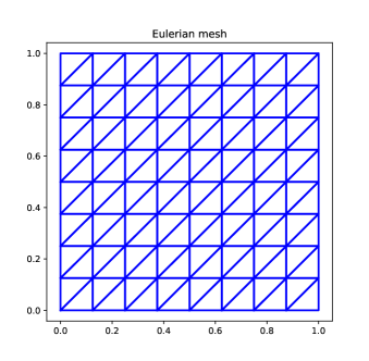
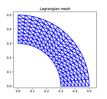
Figure 1. Sketch of the meshes used for the fluid and the structure

The materials properties are $\rho_{f}=1$, $\nu=0.05$, $\delta_{\rho}=0.3$, and $\kappa=1$. The solid mesh size is equal to $1/8$ and the figures show the behavior of the following energy ratio as a function of the time step and of the fluid mesh size

(22) $$\Pi(\mathbf{X}_{h}^{n},\mathbf{u}_{h}^{n})=\frac{\rho_{f}}{2}\|\mathbf{u}_{h}^{n}\|^{2}_{0}+\frac{\delta_{\rho}}{2}\left\|\frac{\mathbf{X}_{h}^{n}-\mathbf{X}_{h}^{n-1}}{\Delta t}\right\|^{2}_{0,\mathcal{B}}+E(\mathbf{X}_{h}^{n}).$$

(a) $\Delta t=10^{-1}$, $h_{x}=1/4$.

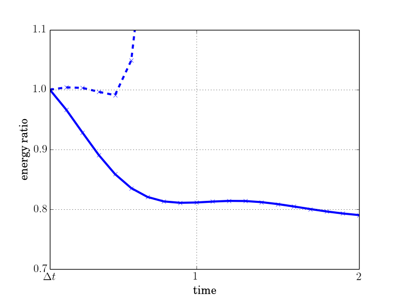
(b) $\Delta t=10^{-1}$, $h_{x}=1/8$.

(c) $\Delta t=10^{-1}$, $h_{x}=1/16$.

(d) $\Delta t=5\cdot 10^{-2}$, $h_{x}=1/4$.

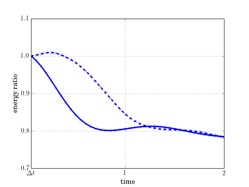
(e) $\Delta t=5\cdot 10^{-2}$, $h_{x}=1/8$.

(f) $\Delta t=5\cdot 10^{-2}$, $h_{x}=1/16$.

Figure 2. Evolution of the quantity $\Pi(\mathbf{X}_{h}^{n},\mathbf{u}_{h}^{n})/\Pi(\mathbf{X}_{h}^{0},\mathbf{u}_{h}^{0})$ (see Equation (22)) for different $\Delta t$ when $h_{x}$ varies. The solid line corresponds to the formulation FE-DLM described in this paper, while the dashed line refers to the FE-IBM scheme which is only conditionally stable

In Table 1 we report the results presented in [15] about the convergence rates in time when different time schemes are used. In these computations the mesh of $\Omega$ is based on a subdivision of $(-1,1)$ in $32$ equal subintervals and the structure is modeled by a Lagrangian mesh obtained by halving the meshsize of the one reported in Figure 1. The fluid is initially at rest and the structure is stretched by a factor $1.4$ in the vertical direction and shrunk by the same factor in the horizontal direction.

The physical parameters are $\rho_{f}=\rho_{s}=1$, $\nu=0.1$, $\kappa=10$, and $T=1$.

We consider BDF1 (semi-implicit backward Euler (11)), BDF2 (see (12)), and two variants of Crank–Nicolson scheme. We denote by CNm the case when the nonlinear terms are evaluated using the midpoint rule and by CNt the case when the trapezoidal rule is used.

The reference solution is calculated by using a smaller timestep with the BDF2 scheme.

Fluid velocity
	BDF1		BDF2		CNm		CNt
$\Delta t$	$L^{2}$ error	rate	$L^{2}$ error	rate	$L^{2}$ error	rate	$L^{2}$ error	rate
$0.05$	$9.18\cdot 10^{-2}$		$3.89\cdot 10^{-2}$		$2.36\cdot 10^{-1}$		$2.39\cdot 10^{-1}$
$0.025$	$5.05\cdot 10^{-2}$	$0.86$	$8.59\cdot 10^{-3}$	$2.18$	$7.54\cdot 10^{-2}$	$1.64$	$7.06\cdot 10^{-2}$	$1.76$
$0.0125$	$2.63\cdot 10^{-2}$	$0.94$	$3.32\cdot 10^{-3}$	$1.37$	$4.24\cdot 10^{-2}$	$0.83$	$2.22\cdot 10^{-2}$	$1.67$
$0.00625$	$1.33\cdot 10^{-2}$	$0.98$	$1.40\cdot 10^{-3}$	$1.24$	$2.19\cdot 10^{-2}$	$0.96$	$4.19\cdot 10^{-3}$	$2.40$

Structure deformation
	BDF1		BDF2		CNm		CNt
$\Delta t$	$L^{2}$ error	rate	$L^{2}$ error	rate	$L^{2}$ error	rate	$L^{2}$ error	rate
$0.05$	$2.03\cdot 10^{-3}$		$7.86\cdot 10^{-4}$		$1.81\cdot 10^{-3}$		$6.51\cdot 10^{-4}$
$0.025$	$1.06\cdot 10^{-3}$	$0.93$	$3.28\cdot 10^{-4}$	$1.26$	$9.75\cdot 10^{-4}$	$0.89$	$1.31\cdot 10^{-4}$	$2.31$
$0.0125$	$5.34\cdot 10^{-4}$	$1.00$	$1.44\cdot 10^{-4}$	$1.18$	$5.10\cdot 10^{-4}$	$0.93$	$4.82\cdot 10^{-5}$	$1.44$
$0.00625$	$2.69\cdot 10^{-4}$	$0.99$	$6.31\cdot 10^{-5}$	$1.19$	$2.55\cdot 10^{-4}$	$1.00$	$1.29\cdot 10^{-5}$	$1.90$

Table 1. Convergence results for the semi-implicit scheme on the fine mesh

We conclude this section by showing the evolution of the structure corresponding to the last example, see Figure 3. A similar example corresponding to a square structure was reported in [8], see Figure 4

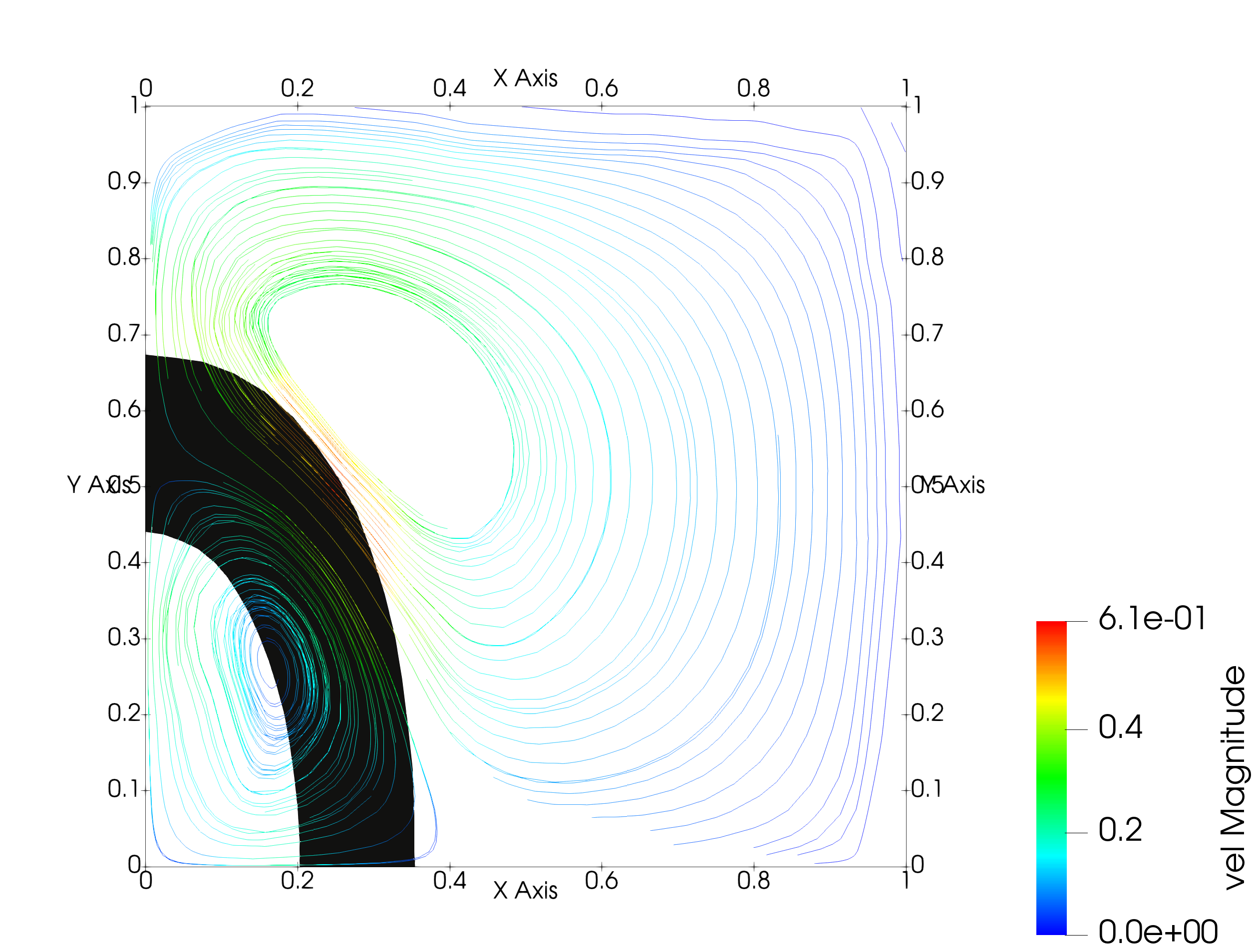
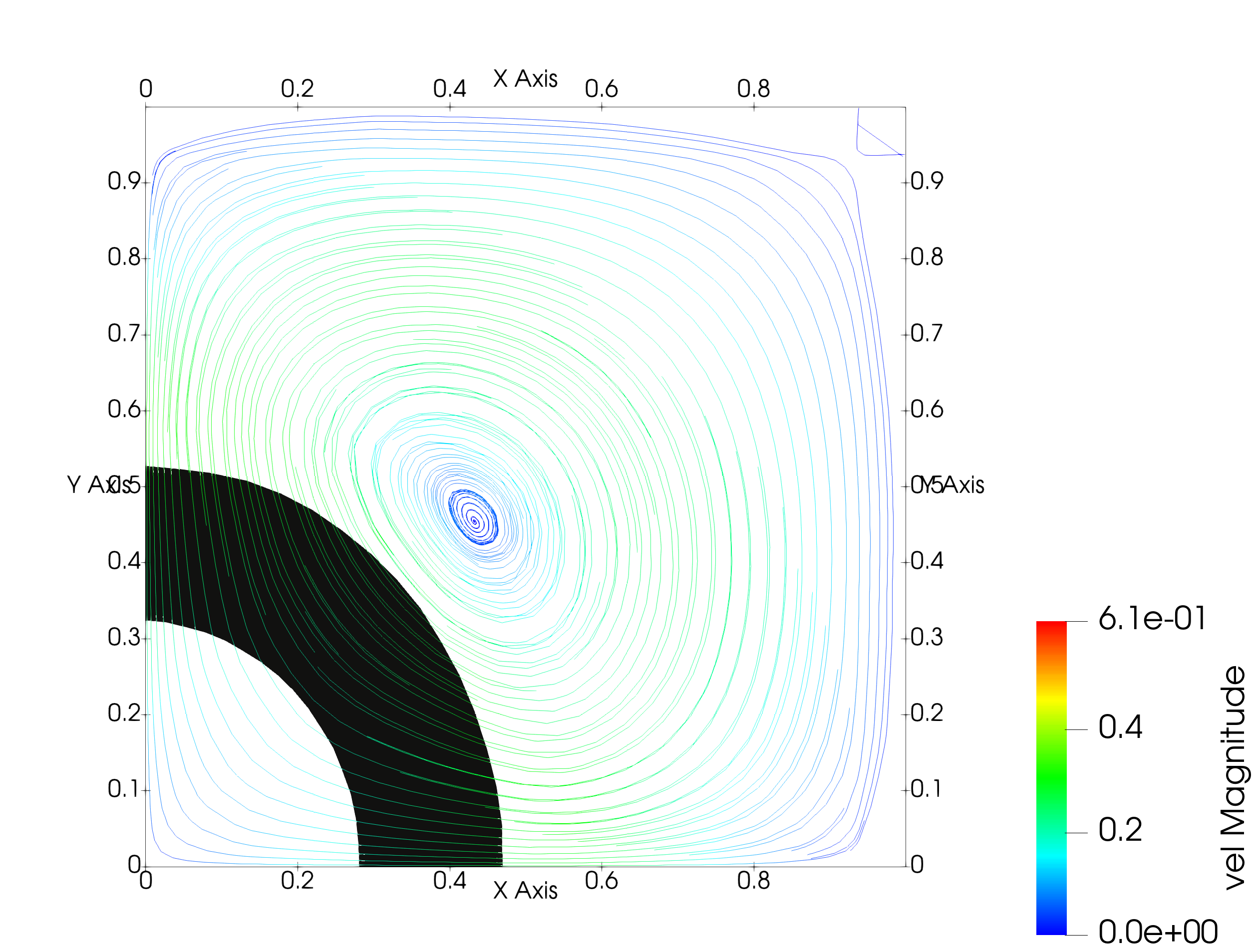
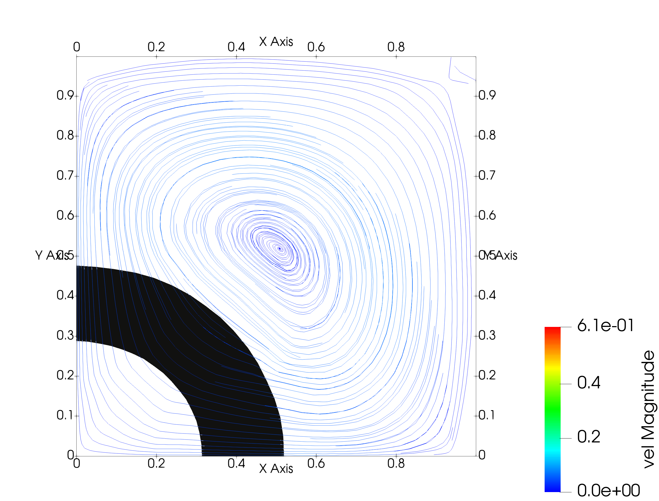
Figure 3. The evolution of an initially deformed ring-shaped structure (computation performed on a quarter of a square for symmetry reasons)

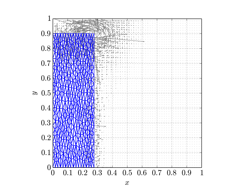
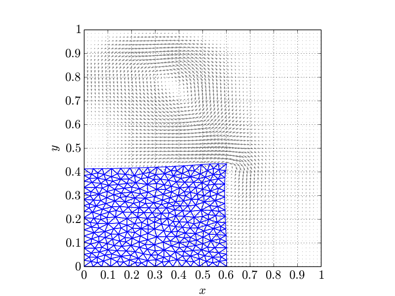
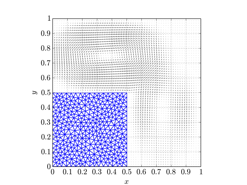
Figure 4. Evolution of an initially deformed square structure immersed in a fluid

References

[1]
Frédéric Alauzet, Benoit Fabrèges, Miguel A. Fernández, and Mikel
Landajuela.
Nitsche-XFEM for the coupling of an incompressible fluid with
immersed thin-walled structures.
Comput. Methods Appl. Mech. Engrg., 301:300–335, 2016.
[2]
Ferdinando Auricchio, Daniele Boffi, Lucia Gastaldi, Adrien Lefieux, and
Alessandro Reali.
On a fictitious domain method with distributed Lagrange multiplier
for interface problems.
Appl. Numer. Math., 95:36–50, 2015.
[3]
H. Beirão da Veiga.
On the existence of strong solutions to a coupled fluid-structure
evolution problem.
J. Math. Fluid Mech., 6(1):21–52, 2004.
[4]
D. Boffi, F. Brezzi, and M. Fortin.
Mixed Finite Element Methods and Applications, volume 44 of
Springer Series in Computational Mathematics.
Springer-Verlag, New York, 2013.
[5]
D. Boffi, N. Cavallini, F. Gardini, and L. Gastaldi.
Local mass conservation of Stokes finite elements.
J. Sci. Comput., 52(2):383–400, 2012.
[6]
D. Boffi, N. Cavallini, and L. Gastaldi.
The finite element immersed boundary method with distributed
Lagrange multiplier.
SIAM J. Numer. Anal., 53(6):2584–2604, 2015.
[7]
D. Boffi, L. Gastaldi, L. Heltai, and C. S. Peskin.
On the hyper-elastic formulation of the immersed boundary method.
Comput. Methods Appl. Mech. Engrg., 197(25-28):2210–2231,
2008.
[8]
Daniele Boffi, Nicola Cavallini, and Lucia Gastaldi.
Advances in the mathematical theory of the finite element immersed
boundary method.
In Giovanni Russo, Vincenzo Capasso, Giuseppe Nicosia, and Vittorio
Romano, editors, Progress in Industrial Mathematics at ECMI 2014, pages
303–310, Cham, 2016. Springer International Publishing.
[9]
Daniele Boffi and Lucia Gastaldi.
A fictitious domain approach with Lagrange multiplier for
fluid-structure interactions.
Numer. Math., 135(3):711–732, 2017.
[10]
Daniele Boffi and Lucia Gastaldi.
A fictitious domain approach with Lagrange multiplier for
fluid-structure interactions.
arXiv:1510.06856v2 [math.NA], 2017.
[11]
Daniele Boffi and Lucia Gastaldi.
On the existence and the uniqueness of the solution to a
fluid-structure interaction problem.
Submitted. arXiv:2006.10536 [math.AP], 2020.
[12]
Daniele Boffi, Lucia Gastaldi, and Luca Heltai.
Numerical stability of the finite element immersed boundary method.
Math. Models Methods Appl. Sci., 17(10):1479–1505, 2007.
[13]
Daniele Boffi, Lucia Gastaldi, and Luca Heltai.
A distributed Lagrange formulation of the finite element immersed
boundary method for fluids interacting with compressible solids.
In Mathematical and numerical modeling of the cardiovascular
system and applications, volume 16 of SEMA SIMAI Springer Ser., pages
1–21. Springer, Cham, 2018.
[14]
Daniele Boffi, Lucia Gastaldi, and Michele Ruggeri.
Mixed formulation for interface problems with distributed Lagrange
multiplier.
Comput. Math. Appl., 68(12, part B):2151–2166, 2014.
[15]
Daniele Boffi, Lucia Gastaldi, and Sebastian Wolf.
Higher-order time-stepping schemes for fluid-structure interaction
problems.
Discrete Contin. Dyn. Syst. Ser. B, 25(10):3807–3830, 2020.
[16]
M. Boulakia and S. Guerrero.
On the interaction problem between a compressible fluid and a
Saint-Venant Kirchhoff elastic structure.
Adv. Differential Equations, 22(1-2):1–48, 2017.
[17]
M. Boulakia, S. Guerrero, and T. Takahashi.
Well-posedness for the coupling between a viscous incompressible
fluid and an elastic structure.
Nonlinearity, 32(10):3548–3592, 2019.
[18]
Erik Burman and Miguel A. Fernández.
An unfitted Nitsche method for incompressible fluid-structure
interaction using overlapping meshes.
Comput. Methods Appl. Mech. Engrg., 279:497–514, 2014.
[19]
P. Causin, J. F. Gerbeau, and F. Nobile.
Added-mass effect in the design of partitioned algorithms for
fluid-structure problems.
Comput. Methods Appl. Mech. Engrg., 194(42-44):4506–4527,
2005.
[20]
A. Chambolle, B. Desjardins, M. J. Esteban, and C. Grandmont.
Existence of weak solutions for the unsteady interaction of a viscous
fluid with an elastic plate.
J. Math. Fluid Mech., 7(3):368–404, 2005.
[21]
Y. C. Chang, T. Y. Hou, B. Merriman, and S. Osher.
A level set formulation of Eulerian interface capturing methods for
incompressible fluid flows.
J. Comput. Phys., 124(2):449–464, 1996.
[22]
C. Conca, J. San Martín H., and M. Tucsnak.
Existence of solutions for the equations modelling the motion of a
rigid body in a viscous fluid.
Comm. Partial Differential Equations, 25(5-6):1019–1042, 2000.
[23]
D. Coutand and S. Shkoller.
Motion of an elastic solid inside an incompressible viscous fluid.
Arch. Ration. Mech. Anal., 176(1):25–102, 2005.
[24]
D. Coutand and S. Shkoller.
The interaction between quasilinear elastodynamics and the
Navier-Stokes equations.
Arch. Ration. Mech. Anal., 179(3):303–352, 2006.
[25]
B. Desjardins and M. J. Esteban.
Existence of weak solutions for the motion of rigid bodies in a
viscous fluid.
Arch. Ration. Mech. Anal., 146(1):59–71, 1999.
[26]
B. Desjardins and M. J. Esteban.
On weak solutions for fluid-rigid structure interaction: compressible
and incompressible models.
Comm. Partial Differential Equations, 25(7-8):1399–1413, 2000.
[27]
B. Desjardins, M. J. Esteban, C. Grandmont, and P. Le Tallec.
Weak solutions for a fluid-elastic structure interaction model.
Rev. Mat. Complut., 14(2):523–538, 2001.
[28]
J. Donea, P. Fasoli-Stella, and S. Giuliani.
Lagrangian and eulerian finite element techniques for transient
fluid-structure interaction problems.
Therm and Fluid/Struct Dyn Anal, B, 1977.
cited By 0.
[29]
Jean Donea, Antonio Huerta, J.-Ph. Ponthot, and A. Rodríguez-Ferran.
Arbitrary Lagrangian–Eulerian Methods.
John Wiley & Sons, Ltd, 2004.
[30]
E. Feireisl.
On the motion of rigid bodies in a viscous compressible fluid.
Arch. Ration. Mech. Anal., 167(4):281–308, 2003.
[31]
V. Girault and R. Glowinski.
Error analysis of a fictitious domain method applied to a Dirichlet
problem.
Japan J. Indust. Appl. Math., 12(3):487–514, 1995.
[32]
V. Girault, R. Glowinski, and T.-W. Pan.
A fictitious-domain method with distributed multiplier for the
Stokes problem.
In Applied nonlinear analysis, pages 159–174. Kluwer/Plenum,
New York, 1999.
[33]
R. Glowinski, T.-W. Pan, T.I. Hesla, and D.D. Joseph.
A distributed Lagrange multiplier/fictitious domain method for
particulate flows.
International Journal of Multiphase Flow, 25(5):755 – 794,
1999.
[34]
R. Glowinski, T.-W. Pan, and J. Périaux.
A fictitious domain method for Dirichlet problem and applications.
Comput. Methods Appl. Mech. Engrg., 111(3-4):283–303, 1994.
[35]
R. Glowinski, T.-W. Pan, and J. Périaux.
A fictitious domain method for external incompressible viscous flow
modeled by Navier-Stokes equations.
Comput. Methods Appl. Mech. Engrg., 112(1-4):133–148, 1994.
Finite element methods in large-scale computational fluid dynamics
(Minneapolis, MN, 1992).
[36]
C. Grandmont and Y. Maday.
Existence for an unsteady fluid-structure interaction problem.
M2AN Math. Model. Numer. Anal., 34(3):609–636, 2000.
[37]
M. D. Gunzburger, H.-C. Lee, and G. A. Seregin.
Global existence of weak solutions for viscous incompressible flows
around a moving rigid body in three dimensions.
J. Math. Fluid Mech., 2(3):219–266, 2000.
[38]
C. W. Hirt, A. A. Amsden, and J. L. Cook.
An arbitrary Lagrangian-Eulerian computing method for all flow
speeds [J. Comput. Phys. 14 (1974), no. 3, 227–253].
volume 135, pages 198–216. 1997.
[39]
K.-H. Hoffmann and V. N. Starovoitov.
On a motion of a solid body in a viscous fluid. Two-dimensional
case.
Adv. Math. Sci. Appl., 9(2):633–648, 1999.
[40]
Thomas J. R. Hughes, Wing Kam Liu, and Thomas K. Zimmermann.
Lagrangian-Eulerian finite element formulation for incompressible
viscous flows.
Comput. Methods Appl. Mech. Engrg., 29(3):329–349, 1981.
[41]
J.-L. Lions and E. Magenes.
Non-homogeneous boundary value problems and applications. Vol.
I.
Springer-Verlag, New York-Heidelberg, 1972.
[42]
B. Muha and S. Čanić.
Existence of a weak solution to a nonlinear fluid-structure
interaction problem modeling the flow of an incompressible, viscous fluid in
a cylinder with deformable walls.
Arch. Ration. Mech. Anal., 207(3):919–968, 2013.
[43]
B. Muha and S. Čanić.
Existence of a weak solution to a fluid-elastic structure interaction
problem with the Navier slip boundary condition.
J. Differential Equations, 260(12):8550–8589, 2016.
[44]
Elijah P. Newren, Aaron L. Fogelson, Robert D. Guy, and Robert M. Kirby.
Unconditionally stable discretizations of the immersed boundary
equations.
J. Comput. Phys., 222(2):702–719, 2007.
[45]
C. S. Peskin.
The immersed boundary method.
Acta Numer., 11:479–517, 2002.
[46]
J.-P. Raymond and M. Vanninathan.
A fluid-structure model coupling the Navier-Stokes equations and
the Lamé system.
J. Math. Pures Appl. (9), 102(3):546–596, 2014.
[47]
D. Serre.
Chute libre d’un solide dans un fluide visqueux incompressible.