Abstract

Post-deployment monitoring of ML systems is critical for ensuring reliability, especially as new user inputs can differ from the training distribution. Here we propose a novel approach, MLDemon, for ML Deployment monitoring. MLDemon integrates both unlabeled data and a small amount of on-demand labels to produce a real-time estimate of the ML model’s current performance on a given data stream. Subject to budget constraints, MLDemon decides when to acquire additional, potentially costly, expert supervised labels to verify the model. On temporal datasets with diverse distribution drifts and models, MLDemon outperforms existing approaches. Moreover, we provide theoretical analysis to show that MLDemon is minimax rate optimal for a broad class of distribution drifts.

1 INTRODUCTION

When ground-truth labels are not readily available at deployment time, which is often the case if labels are expensive, the most common solution is to use an unsupervised, feature-based anomaly detector (Lu et al.,, 2018; Rabanser et al.,, 2018). In some cases, these detectors work well. However, they may also fail catastrophically since it is possible for model accuracy to fall precipitously without possible detection in just the features. This can happen in one of two ways. First, for high-dimensional data, feature detectors may simply lack a sufficient number of samples to detect all covariate drifts. Second, it is possible that drift only occurs in the conditional distribution of the label $y$ given the features $x$ (this can not be detected without supervision). One potential approach, proposed in Yu et al., (2018), applies statistical tests to estimate a change in distribution in the features and then requests expert labels only when such a change is detected. While it is natural to assume that a distribution drift in features should be indicative of a drift in the model's accuracy, in reality feature drift is neither necessary nor sufficient as a predictor of accuracy drift In fact, we find that unsupervised anomaly detectors are often brittle. Thus, any monitoring policy that only triggers supervision from feature-based anomaly can fail both silently and catastrophically.

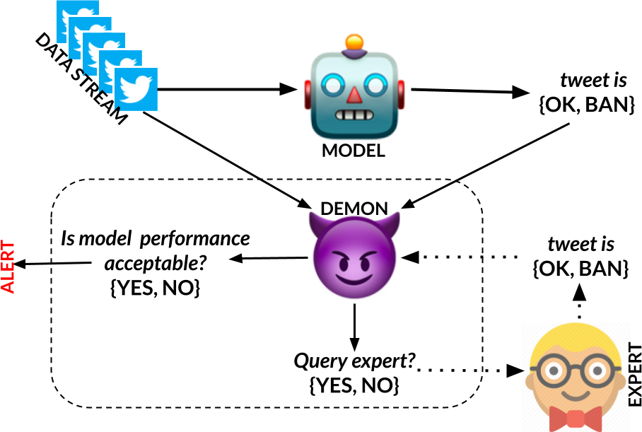
Figure 1: A schematic for the deployment monitoring workflow. For example, an ML system could be deployed to help automate content moderation on a social media platform. In real-time, a trained model determines if a post or tweet should result in a ban. A human expert content moderator can review if the content has been correctly classified by the model, though this review is expensive. A deployment monitoring (demon) policy prioritizes expert attention by determining when tweets get forwarded to the expert for labeling. The demon policy also estimates the model performance during deployment which can be used to alert stakeholders if the model performance is not acceptable.

Deployment monitoring is a vast topic. In this work, we focus on a particular streaming setting where an automated deployment monitoring policy can query experts for labels during deployment (Fig. 1). The goal of the policy is to estimate the model's real-time accuracy throughout deployment while querying the fewest amount of expert labels. Of course, these two objectives are in contention. We seek to design a policy that can effectively prioritize expert attention at key moments. We focus strictly on monitoring, and do not consider policies that automatically update or debug the deployed model.

Contributions

Our contributions are three-fold.

(1) We provide a new mathematical formulation of the ML deployment monitoring problem which is tractable and captures the key trade-off between monitoring cost and risk.

(2) We theoretically prove that our proposed adaptive monitoring policy, MLDemon, is minimax rate optimal up to logarithmic factors and is superior to prior techniques.

(3) Our experiments reveal that feature-based anomaly detectors can be brittle with respect to real distribution shifts and that MLDemon simultaneously provides robustness to errant detectors while reaping the benefits of informative detectors.

2 PROBLEM FORMULATION

We consider a novel online streaming setting (Munro and Paterson,, 1980; Karp,, 1992), where for each time point $t=1,2,\cdots,T$, the data point $X_{t}\in\mathcal{X}$ and the corresponding label $Y_{t}\in\{0,1\}$ are generated from a distribution that may vary over time: $(X_{t},Y_{t})\sim P_{t}$. For a given model $f:\mathcal{X}\rightarrow\{0,1\}$, let $\mu_{t}=\mathbf{Pr}[f(X_{t})=Y_{t}]$ denote its accuracy at time $t$. The total time $T$ can be understood as the life-cycle of the model as measured by the number of user queries. In addition, we assume that we have an anomaly detector, which can depend on both present and past observations and is potentially informative of the accuracy $\mu_{t}$. For example, the detector can quantify the distributional shift of the feature stream $\{X_{t}\}$ where a large drift may imply a deterioration of the model accuracy.

We consider scenarios where high-quality labels $\{Y_{t}\}$ are costly to obtain and are only available upon request from an expert. Therefore, we wish to monitor the model performance $\mu_{t}$ over time while obtaining a minimum number of labels. We consider two settings that are common in machine learning deployments: 1) point estimation of the model accuracy $\mu_{t}$ across all time points (estimation problem), 2) determining if the model's current accuracy $\mu_{t}$ is above or below a user-specified threshold $\rho$ (decision problem). At time $t$, the policy receives a data point $X_{t}$ and submits a pair of actions $(a_{t},\hat{\mu}_{t})$, where $a_{t}\in\{0,1\}$ denotes whether or not to query for an expert label on $X_{t}$ and $\hat{\mu}_{t}$ is the estimate of the model's current accuracy.

It is desirable to balance two types of costs: the average number of queries $Q=\frac{1}{T}\sum_{t}a_{t}$ and the monitoring risk.

In the estimation problem we consider the mean absolute error (MAE) for the monitoring risk:

$$R_{\text{mae}}=\frac{1}{T}\sum_{t}|\hat{\mu}_{t}-\mu_{t}|.$$ (1)

In the decision problem, we consider a binary version $R_{\text{bin}}$ and a continuous version $R_{\text{hinge}}$ for the monitoring risk:

$$R_{\text{bin}}=\frac{1}{T}\sum_{t}\mathfrak{R}_{t},\leavevmode\nobreak\ \leavevmode\nobreak\ \leavevmode\nobreak\ \leavevmode\nobreak\ R_{\text{hinge}}=\frac{1}{T}\sum_{t}|\rho-\mu_{t}|\mathfrak{R}_{t}$$ (2)

where $\mathfrak{R}_{t}=\mathbf{1}\{\mu_{t}>\rho,\hat{\mu}_{t}<\rho\}+\mathbf{1}\{\mu_{t}<\rho,\hat{\mu}_{t}>\rho\}$ is $1$ if the predicted accuracy $\hat{\mu}_{t}$ and the true accuracy $\mu_{t}$ incur different decisions when compared to the threshold $\rho$. We use $R$ to denote the monitoring risk in general when there is no need to distinguish between the risk functions. Therefore, the combined loss Lagrangian (Luenberger et al.,, 1984) can be written as: $\mathcal{L}=cQ+R,$ where $c$ indicates the cost per label query and controls the trade-off between the two types of loss. This Lagrangian implicitly amortizes the query costs and monitoring risks over time. Our goal is to design a policy to minimize the expectation of this amortized loss: $\mathbb{E}_{P}[\mathcal{L}]$.

Assumption on Distributional Drift

We are interested in settings for which the distribution $P_{t}$ varies in time. Without any assumption about how $P_{t}$ changes over time, it is impossible to guarantee that any labeling strategy achieves reasonable performance. Fortunately, many real-world data drifts tend to be more gradual over time. Many ML systems can process hundreds or thousands of user queries per hour, while many real-world data drifts tend to take place over days or weeks. Motivated by this, we consider distribution drifts that are Lipschitz-continuous (O'Searcoid,, 2006) over time in total variation (Villani,, 2008): $\mathcal{P}=\{\{P_{t}\}_{t=1}^{T}:d_{\text{TV}}(P_{t},P_{t-1})\leq\Delta,\forall t\}$. The $\Delta$-Lipschitz constraint captures that the distribution shift must happen in a way that is controlled over time, which is a natural assumption for many cases. The magnitude of $\Delta$ captures the inherent difficulty of the monitoring problem; a small $\Delta$ indicates that the deployment is easier to monitor because the stream drifts slowly. For our theory, we focus on asymptotic regret, in terms of $\Delta$, but amortized over the length of the deployment $T$. While our theoretical analysis relies on the $\Delta$-Lipschitz assumption, our algorithm does not require it to work well empirically.

Feature-Based Anomaly Detection

We assume that our policy has access to a feature-based anomaly detector that computes an anomaly signal from the online feature stream. We let $G_{t}$ denote the anomaly detection signal at time $t$. In practice, most anomaly detectors combine a domain-specific summary statistic (or representation) for dimensionality reduction with a statistical metric for testing for drifts in summary statistics (see Rabanser et al., (2018); Yu et al., (2018); Wang et al., (2019); Pinto et al., (2019); Kulinski et al., (2020); Xuan et al., (2020) for recent examples). Following this general scheme for anomaly detection, we define summary representation $E:\mathcal{X}\rightarrow\mathbb{R}^{s}$ with dimensionality $s$ that embeds the features in a semantically useful space and (generalized) statistical metric $\mathsf{d}:\mathbb{P}(\mathbb{R}^{s})\times\mathbb{P}(\mathbb{R}^{s})\rightarrow\mathbb{R}^{+}$ where $\mathbb{P}(\mathbb{R}^{s})$ denotes the set of all distributions over $\mathbb{R}^{s}$. For any two detection windows $S,S^{\prime}\subset[t]$, we define the detection function $g$:

$$g(S,S^{\prime})=\mathsf{d}\left(\hat{E}(S),\hat{E}(S^{\prime})\right)$$ (3)

where $\hat{E}(S)$ denotes the empirical distribution of $\{E(X_{s}):s\in S\}$. At each time $t$, the policy is responsible for providing the detector with the choice of the two detection windows $(S_{t},S^{\prime}_{t})$ and the anomaly detection signal returns $G_{t}=g(S_{t},S^{\prime}_{t})$. For example, if $\mathsf{d}(P,Q)=||\mathbb{E}{P}-\mathbb{E}{Q}||$, then the anomaly signal $G_{t}$ is equivalent (up to monotonic transformation) to a $Z$-test's $p$-value (Montgomery et al.,, 2009) over the detection windows, and if $\mathsf{d}$ is KS-distance (Naaman,, 2021), then $G_{t}$ is equivalent a KS-test's $p$-value (Lilliefors,, 1967). Common summary representations $E$ include embedding layers of deep neural models or even just the model confidence.

Linear Detection Condition

The core idea of MLDemon is to combine the information from the expert labels and the detection signal based on the feature stream. Practically speaking, any policy that outright ignores the detector is clearly wasting that side information. On the other hand, any policy that blindly trusts the detector is not robust to model assumption violations. MLDemon strikes a balance between these two extreme positions. There is no universal answer as to how this balance should be struck, as it clearly depends on the particular nature of the detector, drift and problem instance in question. However, it is reasonable to assume that for a well-designed detector (i.e., appropriate choices of $E$ and $\mathsf{d}$), for at least a reasonable fraction of instances, the anomaly signal should roughly correlate with the accuracy drift: $|\mu_{t}-\mu_{t^{\prime}}|\approx w\mathsf{d}(E(X_{t}),E(X_{t^{\prime}}))$ for some (unknown) constant $w$. The motivating intuition is that the anomaly signal often correlates with the (absolute) accuracy drift. When this is true, one should expect to be able to fit a linear model to partially capture the relationship even if the true relationship is not exactly linear. We do not require the linear model to always hold; given enough evidence against it, MLDemon learns to discard the assumption. We more formally encode this intuition as the linear detection condition:

Definition 2.1.

(Linear Detection Condition) The linear detection condition holds if with probability at least $q$, for all $S,S^{\prime}$:

$$|\mu(S)-\mu(S^{\prime})|=wg(S,S^{\prime})+\mathcal{N}$$ (4)

where $\mu(S)=\frac{1}{|S|}\sum_{s\in S}\mu_{s}$, $\mathcal{N}$ is an independent and identically distributed zero-mean Gaussian perturbation of arbitrary variance, and $w$ is an arbitrary constant.

This condition is used for theoretical insights of the proposed algorithm rather than a strictly required assumption. That the condition holds probabilistically is a statement about the assumed distribution over problem instances (and in particular about the relationship between $\{P_{t}\}$ and $\{G_{t}\}$ ) that the policy will encounter.

3 Algorithms

We present MLDemon along with two baselines. The first baseline, Periodic Querying (PQ), is a simple non-adaptive policy that periodically queries labels in batches according to a predetermined schedule. The second baseline, Request-and-Reverify (RR), proposed in Yu et al., (2018), is the previous state-of-art to our problem (code sketch in Alg. 2). All of the policies run in constant space and amortized constant time — an important requirement for a scalable long-term monitoring system.

Periodic Querying

works for both the estimation problem and the decision problem. As shown in Alg. 1, given a budget $B$ for the average number of queries per round, PQ periodically queries for a batch of $n$ labels in every $\frac{n}{B}$ rounds, and uses the estimate from the current batch of labels for the entire period.

Inputs: At each time $t$, the previously observed data points and queried labels

Outputs: At each time $t$, $a_{t}\in\{0,1\}$, $\hat{\mu}_{t}\in[0,1]$

Hyperparameters: Window length $n$, budget $B\in[0,1]$

  do:

1. Query ($a_{t}\leftarrow 1$) for $n$ consecutive labels and then do not query ($a_{t}\leftarrow 0$) for $(1/B-1)n$ rounds

2. Compute $\hat{\mu}_{t}$ from most recent $n$ labels as empirical mean

  repeat

Algorithm 1 Periodic Querying

Request-and-Reverify

sets a predetermined threshold $\phi\geq 0$ for anomaly signal $G_{t}$ and queries for a batch of $n$ labels whenever the threshold is exceeded by the anomaly signal $G_{t}\geq\phi$. As for the anomaly detector, RR applies a statistical test on a sliding window of model confidence scores. As discussed in Section 2, the choice of test corresponds to a particular statistical distance $\mathsf{d}$. By varying the threshold $\phi$, RR can vary the number of labels queried in a deployment. In optimistic circumstances, RR is the essentially optimal policy. For example, consider the problem instance: $\mu_{t}=1$ for $t<\tau$, $\mu_{t}=0$ for $t\geq\tau$, and $G_{t}=1$ at $t=\tau$, $G_{t}=0$ otherwise. On the other hand, while training data can be used to calibrate the threshold, in our theoretical analysis we show that for any $\Delta>0$, RR cannot provide a non-trivial worst-case guarantee for monitoring risk, regardless of the choice of anomaly detector. This worst-case is realized when the detector is errant.

Inputs: At each time $t$, the previously observed data points and queried labels, and anomaly signal $G_{t}$

Outputs: At each time $t$, $a_{t}\in\{0,1\}$, $\hat{\mu}_{t}\in[0,1]$

Hyperparameters: Window length $n$, threshold $\phi$

  $G_{t}\leftarrow\text{Compute anomaly score}$

  if $G_{t}\geq\phi$ and not currently querying  then

     (1) Query ($a_{t}\leftarrow 1$) for a batch of $n$ consecutive labels

     (2 $\hat{\mu}_{t}\leftarrow$ empirical mean of $n$ most recent observed outcomes

  else

     Do not query for labels ($a_{t}\leftarrow 0$) and keep $\hat{\mu}_{t}$ fixed

  end if

Algorithm 2 Request-and-Reverify

Detection Windows

Recall that any policy specifies two detection windows at each time, $S_{t},S^{\prime}_{t}$. PQ does not use the anomaly signal, and thus the detection windows are irrelevant. For RR and MLDemon, it is natural in both cases to use the same strategy, defined in Alg. 3.

Hyperparameters: Window length $n$

Outputs: At each time $t$, detection windows $S_{t},S^{\prime}_{t}\subset[t]$

  $\tau\leftarrow\text{time since most recent query batch}$

  $S_{t}\leftarrow\{t-\tau-n,\dots,t-\tau\}$

  $S^{\prime}_{t}\leftarrow\{t-n,\dots,t\}$

  return $(S_{t},S^{\prime}_{t})$

Algorithm 3 Detection Windows

MLDemon

follows a periodic query cycle like PQ. However, MLDemon also fits and evaluates a linear estimate of the accuracy drift based on the anomaly signal. If and when MLDemon becomes sufficiently confident in the model, MLDemon will extend the period in between querying if the anomaly signal yields enough evidence that the model accuracy is sufficiently stable. MLDemon does this by independently generating confidence intervals around $\hat{\mu}_{t}$ based on both the expert labels and on the anomaly signal. MLDemon then combines these independent intervals with Bayes rule (Tipping,, 2003). We think of Alg. 4 as a routine that runs at each time $t$.

As discussed, $E$ and $\mathsf{d}$ are considered part of the problem instance via the given detector. Thus, one of MLDemon's jobs is to select detection windows $(S_{t},S^{\prime}_{t})$ (see Alg. 3). Whenever a new batch of label queries is completed, MLDemon has a good estimate of $\hat{u}_{t}$, and thus it is a good time to fit the linear detection model using the anomaly signal. Concretely, MLDemon applies an ordinary least squares (OLS) update to $\hat{w}$ based on $(G_{t},\partial_{t}\mu)$ where $\partial_{t}\mu=|\hat{\mu}(S_{t})-\hat{\mu}(S^{\prime}_{t})|$.

Inputs: Anomaly signal $\{G_{t}\}$, point estimate history $\{\hat{\mu}_{t}\}$,

Outputs: At each time $t$, action $a_{t}\in\{0,1\}$, accuracy estimate $\hat{\mu}_{t}\in[0,1]$

Hyperparameters: Batch size $n$, risk tolerance $\epsilon$, query period $\alpha$, drift bound $\Delta$, linear detection prior $q$

  $N\leftarrow 0$

  do:

1. Query ($a_{t}\leftarrow 1$) for $n$ consecutive labels and then do not query ($a_{t}\leftarrow 0$) for $\alpha\cdot n$ rounds

2. compute $\hat{\mu}_{t}$ from the most recent $n$ labels as empirical mean

  if At the end of a query period then

     $S\leftarrow\{\text{previous label batch}\}$

     $S^{\prime}\leftarrow\{\text{current label batch}\}$

     $G_{t}\leftarrow g(S,S^{\prime})$

     $\partial_{t}^{\mu}\leftarrow|\hat{\mu}(S)-\hat{\mu}(S^{\prime})|$

     $\hat{w}_{t}\leftarrow\text{OLS update on }\hat{w}_{t-1}\text{ given new data point }(G_{t},\partial_{t}^{\mu})$

     $N\leftarrow N+1$

  end if

  if At the end of a do-not-query period then

     $\mathsf{se}_{t}\leftarrow\text{std. err. of the forecast \cite[citep]{(\@@bibref{AuthorsPhrase1Year}{buteikis2019practical}{\@@citephrase{, }}{})} using OLS}$

     $\tau\leftarrow\text{time since most recent query}$

     $G_{t}\leftarrow\text{Compute anomaly score}$

     $\nu_{t}\leftarrow\Delta\cdot(\tau+(n+1)/2)$

     if decision problem then

        $\ell_{t}\leftarrow\max\{|\hat{\mu}_{t}-\rho|-\epsilon,0\}/\Delta$

     else

        $\ell_{t}\leftarrow 0$

     end if

     $p_{\text{lbl}}\leftarrow 1-2\exp(-2n(\nu_{t}-\epsilon+\ell_{t}-n\Delta)^{2})$

     $p_{\text{det}}\leftarrow 2-2\cdot\mathtt{Student\_t\_cdf\_with\_(N-2)\_deg\_of\_freedom}\left(\frac{\epsilon+\ell_{t}-n\Delta}{\mathsf{se}_{t}}\right)$

     $p_{t}\leftarrow q\left(\frac{p_{\text{lbl}}p_{\text{det}}}{p_{\text{lbl}}p_{\text{det}}+(1-p_{\text{lbl}})(1-p_{\text{det}})}\right)+(1-q)p_{\text{lbl}}$

     if $p_{t}\geq 1-\epsilon$ and $\epsilon-\nu_{t}+\ell_{t}-n\Delta>0$ then

        Extend the do not query period by 1:

        $a_{t}\leftarrow 0$

     else

        End the do not query period and begin to query:

        $a_{t}\leftarrow 1$

     end if

  end if

  repeat

Algorithm 4 MLDemon

MLDemon aggregates the information from recent labels with the anomaly signal from the detector to yield confidence intervals around $\hat{\mu}_{t}$. The label information, via the queries, is used to construct an $\epsilon$-width interval at confidence level $1-p_{\text{lbl}}$ (that is what $\ell_{t}$ and $\nu_{t}$ are used for). The precise formula used to compute $p_{\text{lbl}}$ is based on our novel extension of Hoeffding's Inequality to $\Delta$-Lipschitz setting (see Appendix). The feature information, via anomaly detection signal, is used to construct an $\epsilon$-width interval at confidence level $1-p_{\text{det}}$ (assuming the linear detection condition). The precise formula used to compute $p_{\text{det}}$ is based on the standard prediction interval using a Student-t distribution (which is valid when $\mathcal{N}$ is Gaussian). These two intervals are independent and can be combined with the Bayes rule using the prior $q$ to obtain the joint confidence level $p_{t}$.

The anomaly signal may not correlate with changes in the model's accuracy, so we would also like to incorporate some robustness to counteract the possible failure event of an uninformative or errant detector. Therefore, MLDemon treats $q$ as a hyperparameter that encodes the system's prior belief in the informativeness of the detection signal. Even if the $q$ given to MLDemon is incorrect, MLDemon will still behave reasonably. Unlike RR, MLDemon never assumes the detector is trustworthy, even if $q\leftarrow 1$. MLDemon only trusts the detector it verifies that the detector predicts the drift in $\hat{\mu}$.

For MLDemon, the key variables are (1) monitoring risk tolerance $\epsilon$ that is a desired upper bound on $\mathbb{E}[R]$, (2) the window length for batches of label queries, (3) the query rate, given by $\Theta(1/\alpha)$ for $\alpha\geq 1$, and (4) a Lipschitz constant on the drift, $\Delta$. To deploy MLDemon one must specify two out of $(\epsilon,\Delta,n,\alpha)$. One could also specify $q$ as the prior for the linear detection condition, but, as we shall see, $q\leftarrow 1-\epsilon$ is also a solid choice theoretically and empirically. Upon specifying these two variables as hyperparameters, MLDemon can automatically solve for the remaining two (see Appendix for more details concerning hyperparameter selection).

For the decision problem, we can additionally increase the query period based off the estimated margin to the target threshold using our estimate of $|\hat{\mu}_{t}-\rho|$. With a larger margin, we need a looser confidence interval to guarantee the same monitoring risk. This translates into fewer label queries while still preserving a risk tolerance upper bound of $\epsilon$.

4 Theoretical Analysis

Minimax Analysis

Our asymptotic analysis in this section is concerned with an asymptotic rate in terms of small $\Delta$ and amortized by a large $T$. When using asymptotic notation, by loss $\mathcal{L}=O(\Delta^{k})$ we mean $\lim_{\Delta\rightarrow 0}\lim_{T\rightarrow\infty}\mathcal{L}\leq c_{0}\Delta^{k}$, for some constant $c_{0}>0$. Recall that amortization is implicit in the definition of $\mathcal{L}=cQ+R$ (defined in Section 2). We use tilde notation (for example, $\widetilde{O}$) to denote the omission of logarithmic factors. We let $\mathcal{L}_{g}^{\pi}$ be the combined loss when using policy $\pi$ and anomaly detector $g$. Recall that a detector $g$ is defined by representation $E$ and statistical distance $\mathsf{d}$. When using MAE risk, we only consider estimation problems, and when using hinge risk, we only consider decision problems. All the proofs are in the appendix.

Theorem 4.1.

Let $\mathcal{P}=\mathbf{Lip}(\Delta)$ be the set of $\Delta$-Lipschitz drifts and let $\Pi$ be the space of deployment monitoring policies. For both MAE risk and hinge risk, for any model $f$ and anomaly detector $g$:

(i) PQ has a worst-case expected loss $\sup_{P\in\mathcal{P}}\mathbb{E}_{P}[\mathcal{L}^{\mathbf{PQ}}_{g}]=\widetilde{O}\big{(}\Delta^{1/4}\big{)}$ ;

(ii) When $0\leq q<1$ is constant and $\epsilon=\Theta(\Delta^{1/4})$, MLDemon has a worst-case expected loss $\sup_{P\in\mathcal{P}}\mathbb{E}_{P}[\mathcal{L}^{\mathbf{MLD}}_{g}]=\widetilde{O}\big{(}\Delta^{1/4}\big{)}$;

(iii) RR has a worst-case expected loss $\sup_{P\in\mathcal{P}}\mathbb{E}_{P}[\mathcal{L}^{\mathbf{RR}}_{g}]=\Theta(1)$;

(iv) No policy can achieve a better worse-case expected loss than MLDemon and PQ: $\inf_{\pi}\text{ }\sup_{P}\mathbb{E}_{P}[\mathcal{L}^{\pi}_{g}]=\Omega\left(\Delta^{1/4}\right)$.

MLDemon is minimax rate optimal up to logarithmic factors. This analysis treats MLDemon's $q$ as a non-asymptotic hyperparameter, but Thm. 4.1 does not assume the linear detection condition. In contrast to the robustness of MLDemon, RR can fail catastrophically with any detector. For hard problem instances, the anomaly signal is errant and the threshold margin is small, so MLDemon cannot outperform PQ from a minimax perspective.

Lemma 4.2.

Under the conditions of Thm. 4.1, for both MAE and hinge risk, PQ and MLDemon achieve a worst-case expected monitoring risk of $O(\epsilon)$ with a query rate of $O(\frac{\Delta\log(1/\epsilon)}{\epsilon^{3}})$ and no policy can achieve a query rate of $\omega(\Delta/\epsilon^{3})$ with monitoring risk $O(\epsilon)$.

Lem. 4.2 is used to prove Thm. 4.1, but we include it here because it is of independent interest to understand the trade-off between monitoring risk and query costs and it also gives intuition for Thm. 4.1. The emergence of the $\Delta^{1/4}$ rate also follows from Lem. 4.2 by considering the combined loss $\mathcal{L}$ optimizing over $\epsilon$ to minimize $\mathcal{L}$ subject to the constraints imposed by Lem. 4.2. Lem. 4.2 itself follows from an analysis that pairs a lower bound derived with Le Cam's method (Yu,, 1997) and an upper bound constructed with an extended Hoeffding's inequality (Hoeffding,, 1994) that handles samples with $\Delta$-Lipschitz drift.

Optimistic Analysis

We investigate how much MLDemon can improve over PQ by using the linear detection condition. When it holds with probability $q$, MLDemon can guarantees a worst-case monitoring risk $\epsilon$ while reducing the labeling rate significantly if: (i) the noise magnitude of $\mathcal{N}$ is small and (ii) the accuracy drift $\{\mu_{t}\}$ is stable. Condition (i) enables MLDemon to fit the linear model with low forecast error and condition (ii) enables MLDemon to extend the query period since the policy can confidently forecast that $\{\mu_{t}\}$ is not drifting. For the following theorem, it will be useful to recall that $Q^{\mathbf{PQ}}=\sup_{P\in\mathcal{P}}\mathcal{Q}^{\mathbf{MLD}}_{g}$ since MLDemon only ever reduces the query rate compared to PQ.

Theorem 4.3.

Under the conditions of Thm. 4.1, the following hold if, additionally, $(E,\mathsf{d})$ satisfies the linear detection condition with probability $q$:

(i) if using MAE risk and $q<1-\epsilon$ then,

$$\frac{3}{13}-\widetilde{O}(\Delta^{1/4})\leq\inf_{P\in\mathcal{P}}\mathbb{E}_{P}\left[\frac{\mathcal{Q}^{\mathbf{MLD}}_{g}}{\mathcal{Q}^{\mathbf{PQ}}_{g}}\right]\leq\frac{9}{19}-\widetilde{O}(\Delta^{1/4})$$

(ii) if using hinge risk and $q<1-\epsilon$ then,

$$\inf_{P\in\mathcal{P}}\mathbb{E}_{P}\left[\frac{\mathcal{Q}_{g}^{\mathbf{MLD}}}{\mathcal{Q}_{g}^{\mathbf{PQ}}}\right]=\widetilde{O}(\Delta^{1/4})$$

(iii) if $q\geq 1-\epsilon$, then there exist problem instances $P$ for which $Q_{g}^{\mathbf{MLD}}/Q_{g}^{\mathbf{PQ}}=0$ almost surely.

Thus, there are two regimes for MLDemon. When $q\rightarrow 1$ (part iii), there exist problem instances for which MLDemon exhibits behavior like RR, namely, the possibility of never querying for a label after a certain point in the stream (which is a dangerous behavior). When $q$ is constant (parts i & ii), MLDemon is still minimax rate optimal as stated in Thm. 4.1, but can reduce the number of label queries by up to a factor of about 2-4$\times$ when using MAE risk and $\Delta$ is small and even more so when using hinge risk.

Average-Case Analysis

For the hinge risk, there is gap a in asymptotic query rates for minimax and optimistic situations. To investigate this further, we perform an average-case analysis with a stochastic model implying a distribution over problem instances in $\mathcal{P}$. Our model assumes the following law, denoted as $\mathcal{S}$, for generating the sequence $\{\mu_{t}\}$ from any arbitrary initial condition $\mu_{0}$: $\mu_{t}=\mathbf{min}\{\mathbf{max}\{\mu_{t-1}+\mathbf{Unif}(-\Delta,\Delta),1\},0\}$. The accuracy drift is modeled as a simple random walk. As discussed in Szpankowski, (2011) the maximum entropy principle (used by our model at each time step under the $\Delta$-Lipschitz constraint) is often a reasonable stochastic model for average-case analysis.

Theorem 4.4.

For hinge risk and model $f$, and detector $g$, when $0\leq q<1$ is constant and $\epsilon=\Theta(\Delta^{1/4})$:

$$\frac{\mathbb{E}_{P\sim\mathcal{S}}\mathcal{L}_{g}^{\mathbf{MLD}}}{\mathbb{E}_{P\sim\mathcal{S}}\mathcal{L}_{g}^{\mathbf{PQ}}}\leq\widetilde{O}(\Delta^{1/12})$$

The reason we have a better asymptotic gain in the decision problem is illuminated below in Lem. 4.5.

Lemma 4.5.

For hinge risk under model $\mathcal{S}$, MLDemon achieves an expected monitoring hinge risk $O(\epsilon)$ with an amortized query amount $\widetilde{O}\left(\Delta/\epsilon^{2}\right)$.

MLDemon can save an average $1/\epsilon$ factor in query cost, which translates into the rate improvement in Thm. 4.4. MLDemon does this by leveraging the margin between estimate $\hat{\mu}$ and threshold $\rho$ to increase the confidence interval width around the estimate without increasing risk. Note that when using the minimax optimal hyperparameters $\epsilon=\Theta(\Delta^{1/4})$, then Lem. 4.5 also implies that the expected ratio of query rates behaves like the optimistic ratio: $\mathbb{E}_{\mathcal{S}}[{Q^{\mathbf{MLD}}/Q^{\mathbf{PQ}}}]=\mathbb{E}_{\mathcal{S}}[Q^{\mathbf{MLD}}]/Q^{\mathbf{PQ}}=\widetilde{O}(\Delta^{1/4})$ (see appendix for more details).

5 Experiments

Our asymptotic analysis indicates that MLDemon can achieve robustness close to that of PQ yet also reap the benefits of an informative detector like RR. In this section, we implement the algorithms on real data streams as a proof-of-concept.

Data Streams

We benchmark the 3 policies on 3 data stream benchmarks (summarized below and in Table 1).

(1) SPAM-CORPUS (Katakis et al.,, 2006): A non-stationary data set for detecting spam mail over time based on text. It represents a real, chronologically ordered email inbox from the early 2000s and is a canonical benchmark for non-stationary learning.

(2) WEATHER-AUS: A non-stationary data set for predicting if it will rain in Australia based on other weather and geographic features. The data is gathered from a range of locations and time spanning years.

(3) FACE-R (Wang et al.,, 2020): A data set that contains multiple images of hundreds of individuals, both masked and unmasked. The distribution drift mimics the onset of a pandemic by increasing the percentage of masked individuals. Initially, the masked percentage grows slowly, followed by a sharp increase.

Data Stream Details
Data Stream	$T$	# class	Model	$\mu_{0}$	$\mathsf{se}$	$(\varepsilon_{\min},\varepsilon_{\max})$
SPAM-CORPUS	7,300	2	Logistic Reg.	$92\%$	0.0695	$(0.0674,0.134)$
WEATHER-AUS	45,000	2	Logistic Reg.	$86\%$	0.175	$(0.091,0.134)$
FACE-RECOG	40,000	400	Residual CNN	$38\%$	0.0304	$(0.053,0.097)$

Table 1: Three data streams used in our empirical study. $T$ is the length of the stream in our benchmark. The initial test accuracy on the training distribution at time $t=0$ is denoted by $\mu_{0}$ and standard error of the forecast by an OLS linear model following Eqn. 4 is denoted by $\mathsf{se}$. The minimal and maximal empirical average monitoring risk are denoted by $\varepsilon_{\min}$ and $\varepsilon_{\max}$, respectively. Also reported are the number of classes in the classification task and the classifier used.

Anomaly Detector

Following Yu et al., (2018); Rabanser et al., (2018), for SPAM-CORPUS and WEATHER-AUS, we take let representation $E(X)$ be the model's confidence on a particular data point $X$, as given by the model logits. This is a popular choice and is often the only possible choice when using inference APIs. For FACE-RECOG, we use the face embedding $E(X)$ produced by a residual CNN for face $X$. For the choice of $\mathsf{d}$, we follow Rabanser et al., (2018) and simply take $\mathsf{d}(P,Q)=||\mathbb{E}{P}-\mathbb{E}{Q}||$ (equivalent to a $Z$-test on the empirical means).

The informativeness of the anomaly detection signal is a key aspect of a problem instance. Over the entire stream, we can globally quantify this with the standard error of the forecast (Buteikis,, 2019) (herein denoted $\mathsf{se}$) of an OLS linear fit of the anomaly signal. Smaller $\mathsf{se}$ indicate more accurate predictions from the linear model. While $\mathsf{se}$ is a reasonable global metric, it does not capture all of the nuances. Notice that the realized informativeness of the anomaly signal can depend on the label query rate. Taking RR as an example, suppose $\phi$ is high enough such that it is exceeded but once and RR only queries for one batch of labels. Further suppose that this occurs at the precisely optimal moment given that the policy will only query one batch of labels. For this example, it would seem the detector was highly informative. However, in the same example instance, it could be that even slightly lowering $\phi$ causes RR to make many additional label batch queries at particularly sub-optimal moments (for example, if the stream is not drifting at those moments). At a higher label rate, the same detector may seem mostly uninformative or even outright errant.

Training, Implementation & Hyperparameters

For the logistic regression models, we train models on the first $5\%$ of the drift, then treat the rest as the deployment test. For FACE-R, we use an open-source facial recognition package that is powered by a pre-trained residual CNN (He et al.,, 2015) that computes face embeddings.

Each dataset is a time-series of labeled data $\{(X_{t},Y_{t})\}$. For each dataset, we generate 8 streams by randomly shuffling the data locally. As a proxy for the true $\{\mu_{t}\}$, which is unknown for real data, we use compute a moving average for the empirical $\mu_{t}=\frac{1}{\ell}\sum_{i=0}^{\ell}\mathbf{1}\{f(X_{t-i})=Y_{t-i}\}$ with sliding window length $\ell=250$. For all methods, we fix the label query batch size $n=35$. This was a neutral choice made by tuning for the best batch size for PQ on a synthetic dataset. For PQ, we sweep the amortized query budget $B$. For MLDemon, with $n$ fixed, for consistency with PQ, we choose to sweep query rate parameter $\alpha$. For RR we also sweep the anomaly threshold $\phi$. See Appendix for more details.

(a) Lower monitoring risk: $\eta=0.15$. The baseline avg. query rate for PQ is $7.4\%$ on WEATHER-AUS, $7.1\%$ on SPAM-CORPUS, and $1.3\%$ on FACE-RECOG.

(b) Moderate monitoring risk: $\eta=0.30$. The baseline avg. query rate for PQ is $4.1\%$ on WEATHER-AUS, $6.3\%$ on SPAM-CORPUS, and $0.5\%$ on FACE-RECOG.

Figure 2: Number of label queries needed by PQ, RR, and MLDemon to achieve a target monitoring risk. Each target monitoring risk (MAE) is computed by $\varepsilon=\eta(\varepsilon_{\max}-\varepsilon_{\min})+\varepsilon_{\min}$ for each benchmark. Error bars are interpolated std. err. of the mean.

Minimal and Maximal Monitoring Risk

We define the maximal monitoring risk as $\varepsilon_{\max}=\frac{1}{T}\sum_{{}_{t}}|\mu_{0}-\mu_{t}|$. The maximal monitoring risk serves as a good upper bound for the monitoring risk $R$ because it is the risk of a policy that never queries for a single label and simply relies on the initial test accuracy. Similarly, for a given batch size $n$ (in this case $n=35$), the minimal monitoring risk is defined as $\varepsilon_{\min}=\frac{1}{T}\sum_{{}_{t}}|\frac{1}{\tau}\sum_{\tau=t-n}^{t}Y_{\tau}-\mu_{t}|$. The minimal monitoring risks serves as a good lower bound for $R$ because it the risk of a policy that queries for every single label while using a given batch size for estimating $\hat{\mu}$.

Results (Fig. 2)

MLDemon performs at least as well as PQ and RR, and in some cases, performs significantly better (around a third fewer labels than RR and up to a $40\%$ reduction in labels compared to PQ). When the anomaly detector is errant (as evidenced by RR performing significantly worse than PQ), we MLDemon behaves nearly identically to PQ, because the OLS linear fit is not dependable. If RR performs equivalently to PQ, MLDemon may sometimes also perform equivalently, but might also moderately improve upon both.

On WEATHER-AUS, the $\mathsf{se}$ is not low enough for MLDemon to extend the query period, and thus it behaves like PQ. For low monitoring risk $(\eta=0.15)$, RR behaves comparably, although not identically. At $\eta=0.3$, RR performs poorly. On SPAM-CORPUS, MLDemon is able slightly outperform the baselines at $\eta=0.15$ and more substantially at $\eta=0.3$ (recall that detector quality depends on the query rate and thus the monitoring risk). On FACE-RECOG, the face embeddings tend to have an easily detectable signal as to whether or not the individual is masked, which results in a larger improvement for RR and MLDemon. However, RR fails to detect gradual decreases in accuracy early on in the stream, only querying near the end when the larger transition occurs. MLDemon's surveillance querying captures the slow drifts that might be too gradual for the anomaly signal.

The experimental findings support the theoretical conclusion that it is a risky policy to purely rely on potentially brittle anomaly detection instead of balancing surveillance queries with anomaly-driven queries. Of course, we caution that the quality of the anomaly detector is not the only factor in a policy's performance. The stability of the drift also plays a major role.

6 Discussion

Related Works

While our problem setting is novel, there are a variety of settings relating to ML deployment and distribution drift. One such line of work focuses on reweighting data to detect and counteract label drift (Lipton et al.,, 2018; Garg et al.,, 2020). Another related problem is when one wants to combine expert and model labels to maximize the accuracy of a joint classification system (Cesa-Bianchi et al.,, 1997; Farias and Megiddo,, 2006; Morris,, 1977; Fern and Givan,, 2003). The problem is similar in that some policy needs to decide which user queries are answered by an expert versus an AI, but the problem is different in that it is interesting even in the absence of online drift or high labeling costs. It would be interesting to augment our formulation with a reward for the policy when it can use an expert label to correct a user query that the model got wrong. This setting would combine both the online monitoring aspects of our setting along with ensemble learning (Polikar,, 2012; Minku et al.,, 2009) under concept drift with varying costs for using each classifier depending on if it is an expert or an AI.

Complementary to MLDemon's focus on the supervision-monitoring trade-off is work by Shao et al., (2020) and Pinto et al., (2019), which are more focused on the alerting, explanation, and drift detection aspects of the problem without investigating the supervision-monitoring trade-off. Another related approach, explored in Schelter et al., (2020), is to try to corrupt training data synthetically in order to fit a predictor that generalizes to natural drift in deployment.

Adaptive sampling rates are a well-studied topic in the signal processing literature (Dorf et al.,, 1962; Mahmud,, 1989; Peng and Nair,, 2009; Feizi et al.,, 2010). The essential difference is that in signal processing, measurements tend to be exact whereas in our setting a measurement just reveals the outcome of a single Bernoulli trial. Another popular related direction is online learning or lifelong learning during concept drift. Despite a large and growing body of work in this direction, including (Fontenla-Romero et al.,, 2013; Hoi et al.,, 2014; Nallaperuma et al.,, 2019; Gomes et al.,, 2019; Chen et al.,, 2019; Nagabandi et al.,, 2018; Hayes and Kanan,, 2020; Chen and Liu,, 2018; Liu,, 2017; Hong et al.,, 2018), this problem is by no means solved. Our setting assumes that after some time $T$, the model will eventually be retired for an updated one. It would be interesting to allow a policy to update $f$ based on the queried labels. Model robustness is a related topic that focuses on designing $f$ such that accuracy does not fall during distribution drift (Zhao et al.,, 2019; Lecué et al.,, 2020; Li,, 2018; Goodfellow et al.,, 2018; Zhang et al.,, 2019; Shafique et al.,, 2020; Miller et al.,, 2020).

Broader Impacts & Limitations

Anomaly detectors may be fragile. By robustifying the monitoring process, MLDemon can help organizations and stakeholders safely deploy ML models. MLDemon's limitation is that it lacks the ability to go beyond alert generation. An interesting direction for future work is to incorporate downstream model repair and retraining together with monitoring.

Conclusion & Future Directions

We pose and analyze a novel formulation for studying automated ML deployment monitoring. Understanding the trade-off between expert attention and monitoring quality is of both research and practical interest. Our proposed policy comes with theoretical guarantees and performs favorably on empirical benchmarks. The potential impact of this work is that MLDemon could be used to improve the reliability and efficiency of ML systems in deployment. Since this is a relatively new research direction, there are interesting directions for future work. We have assumed that experts respond to label requests instantly. In the future, we can allow the policy to incorporate labeling delay. Also, we have assumed that an expert label is as good as a ground-truth label. We can relax this assumption to allow for noisy expert labels. We could also let the policy more actively evaluate the apparent informativeness of the anomaly signal over time or even input an ensemble of different anomaly signals and learn which are most relevant at a given time. While MLDemon is robust even if the feature-based anomaly detector is not good, it is more powerful with an informative detector. Improving the robustness of anomaly detectors for specific applications and domains is a promising area of research.

Acknowledgements

We'd like to acknowledge V. Bagaria and B. He for useful conversations about this work. Also, we thank A. Grosskopf for helping with figure design and editorial help with the manuscript. Additionally, we thank the anonymous reviewers for helpful feedback. A.A.G. is supported by a Stanford Bio-X Fellowship. M.J.Z. is supported by NIH R01 MH115676. J.Z. is supported by NSF CAREER 1942926 and funding from the Chan-Zuckerberg Initiative and the Stanford AI Lab.

 

Supplementary Material:
MLDemon:
Deployment Monitoring for Machine Learning Systems

 

Appendix A IMPLEMENTATION DETAILS

A.1 Hyperparameter Selection for MLDemon

First, we describe in more detail the hyperparameter selection for MLDemon. We delve into the quantitative laws that bind the hyperparameters; these ultimately enable MLDemon to automatically select some of the hyperparameters as discussed below.

In total, MLDemon has the following hyperparameters: $n,\alpha,\Delta,\epsilon,\rho$ and $q$. Of these, only two out of $n,\alpha,\Delta$ and $\epsilon$ are to be specified, with the exception of the pair $n,\epsilon$. Recall that $\rho$ specifies the threshold when in a decision problem. Without loss of generality, we let $\rho\geq 1/2$ (if $\rho<1/2$, simply reflect about $1/2$). For most of our analysis, the particular choice of $\rho$ only impacts the key quantities up to a constant factor, and thus we sometimes omit explicit reference to $\rho$ or carry out the analysis with $\rho\leftarrow 1/2$.

Generally, it always makes sense to specify $n$ (the batch size of a the label queries) and $\alpha$ (specifies the ratio of the minimum waiting period in between label batches to the batch size). Based on these selections, MLDemon automatically chooses rate optimal pairs $(\epsilon,\Delta)$ such that if the drift is indeed $\Delta$-Lipschitz, MLDemon will guarantee expected monitoring risk lower than $\epsilon$.

Another practical option is to specify $\epsilon$ and $\alpha$. In this case, MLDemon automatically chooses a batch size $n$ in order to guarantee $\epsilon$ and computes the best possible $\Delta$ for which it can guarantee $\epsilon$ given $n$ and $\alpha$.

In our theoretical analysis, $\Delta$, $q$ and $\rho$ are problem instances parameters. The threshold $\rho$ is known in practice since it is generally set by the system designer. Obviously, in practice, $\Delta$ might not be known (or may not even exist). However, sometimes, $\Delta$ can reasonably be upper bounded from historical trends, in which case one is also free to specify it. Although we do not formally address this here, the results in this paper should also generalize to the case in which the drift is $\Delta$-Lipschitz with high probability.

As for $q$, it is of course not known in practice, but the choice $q\leftarrow 1-\epsilon$ has solid theoretical properties and is recommended.

Law for $n$ as a function of $\epsilon$:

$$n\leftarrow\frac{9\log(2\rho/\epsilon)}{2\epsilon^{2}}$$ (5)

Law for $\epsilon$ as a function of $n$:

$$\epsilon\leftarrow 2\rho\cdot\exp{\left(-\frac{1}{2}W\left(\frac{16n\rho^{2}}{9}\right)\right)}$$ (6)

where $W$ denotes the Lambert-W function (Veberič,, 2012; Valluri et al.,, 2000).

Law relating $\Delta$, $\epsilon$, and $\alpha$:

$$\Delta=\frac{\epsilon^{3}}{15\alpha\log(2\rho/\epsilon)}$$ (7)

Note that these laws are not arbitrary. They are constructed intentionally. Reading the proofs should illuminate them.

A.2 Data Stream Details

We describe each of the eight data streams in greater detail. All data sets are public and may be found in the references. All lengths for each data stream were determined by ensuring that the stream was long enough to capture interesting drift dynamics.

A.2.1 Data Stream Construction

1. SPAM-CORPUS: We take the first $7400$ points from the data in the order that it comes in the data file.

2. WEATHER-AUS: For each random seed, we uniformly at random select of block of length $45,000$ from the data while preserving the chronological the order of the data.

3. FACE-R: We randomly subsample 400 individuals out of the data set that have at least 3 unmasked images and 1 masked image to create a reference set. For these 400 individuals, we begin with a masking fraction of 10%, and at some uniformly at random point in time (for each seed) we increase the masking fraction to 99%. The total duration is 40,000.

A.2.2 Bootstrapping

In order to get iterates for each data set, we generate the stream by bootstrap as follows. We block the data sequence into blocks of length $32$ and uniformly at random permute the data within each block. Because $32\ll T$ this bootstrapping preserves the structure of the drift.

A.3 Models

A.3.1 Logistic Regression

For the logistic regression model, we used the default solver provided in the scikit-learn library (Pedregosa et al.,, 2011). As mentioned in the main text, we compute confidence scores in the usual way, meaning that we just take the logit value. Because these models are shallow, standard training routines produce fairly well calibrated models.

A.3.2 Facial Recognition

For the facial recognition system, we used the open-source model referenced in the main text. The model computes face embeddings given images. The embeddings are then used to compute a similarity score as described in the API. For any query image belonging to one of 400 individuals, the model looks for the best match among the 400 individuals by comparing the query image to each of the 3 reference images for each individual and taking an average similarity score. The highest average similarity score out of the 400 individuals is returned as the predicted matching individual.

Appendix B MATHEMATICAL DETAILS AND PROOFS

We begin with reviewing definitions and notations. We will then proceed with proofs for the results. We strongly recommend reading the proofs in the presented order.

B.1 Definitions & Notation

B.1.1 Problem Instances

Although this we have defined the notion of a problem instance throughout the main text, we briefly but formally revisit this here.

We consider sequences of distributions $\{P_{t}\}$ each over $(X,Y)$ that are $\Delta$-Lipschitz in the sense defined in the main text's problem formulation. Each problem instance has a fixed model $f$ and accuracy at time $t$ given by $\mu_{t}=\mathbf{Pr}[Y_{t}=f(X_{t})]$. Additionally, each problem instance specifies a detection function $g$ that is parameterized by representation $E$ and statistical metric $\mathsf{d}$ (as described in the main text).

Definition B.1.

Space of all Distributions over a Measurable Space

For a given measurable space $\Omega$, we let $\mathbb{P}(\Omega)$ denote the set of all probability distributions over $\Omega$. In the case that $\Omega$ is Euclidean, we assume the standard Borel $\sigma$-algebra.

Definition B.2.

Anomaly Detector

An anomaly detector (or anomaly detection signal) $g$ is pair $(E,\mathsf{d})$ such that $E:\mathcal{X}\rightarrow\mathbb{R}^{s}$ and $\mathsf{d}:\mathbb{P}(\mathbb{R}^{s})\times\mathbb{P}(\mathbb{R}^{s})\rightarrow\mathbb{R}^{+}$. We let $\mathcal{G}$ denote the space of all such possible anomaly detectors.

Additionally, we sometimes may assume the linear detection condition (Def. 2.1) which implicitly is a statement about some assumed distribution over problem statements. In other words, assuming the linear detection condition is like assuming that the problem instance itself is a random variable from a distribution that satisfies some additional constraints but is otherwise unknown.

B.1.2 Initial Model Accuracy

We use the convention that $\mu_{0}$ is known from some held-out data. All policies can make use of this as their initial estimate.

Definition B.3.

Accuracy at time $0$:

$$\hat{\mu}_{0}=\mu_{0}$$ (8)

B.1.3 Monitoring Risk

We first define the instantaneous monitoring risk, $r$ which we distinguish here from the amortized monitoring risk $R$ (defined in the main text). Instantaneous monitoring risk $r$ is the risk for a particular data point whereas $R$ is the amortized risk over the entire deployment.

Definition B.4.

Instantaneous Monitoring Risk

We define the monitoring risks in MAE and hinge settings for a single data point in the stream below.

$$r_{\mathbf{mae}}(\theta,\hat{\theta})=|\theta-\hat{\theta}|$$ (9)

$$r_{\mathbf{hinge}}(\theta,\hat{\theta};\rho)=|\rho-\theta|\left(\mathbf{1}\{\theta>\rho,\hat{\theta}<\rho\}+\mathbf{1}\{\theta<\rho,\hat{\theta}>\rho\}\right)$$ (10)

As mentioned in the main text, we omit the subscript when the loss function is clear from context or is not relevant. In the context of our online problem, at time $t$ for policy $\pi$, we may generally infer that $\theta=\mu_{t}$, $\hat{\theta}=\hat{\mu}_{t}$ and $\rho$ is fixed over time. In this case, we might use the shorthand $r^{\pi}(t)$, as below:

Definition B.5.

Amortized Monitoring Risk

$$R^{\pi}=\frac{1}{T}\sum_{t=1}^{T}r^{\pi}(t)$$ (11)

where $\pi$ is the policy and $R$ is the usual amortized monitoring risk term defined in Section 2.

We may also omit the superscript $\pi$ when the policy is clear from context.

Also recall from Section 2 that we defined the query rate $Q$:

Definition B.6.

Amortized Query Rate

$$Q^{\pi}=\frac{1}{T}\sum_{t=1}^{T}{a_{t}}$$ (12)

where $a_{t}=1$ if the policy queries a label at time $t$ and $a_{t}=0$ otherwise.

Definition B.7.

Policy Loss

$$\mathcal{L}=R+cQ$$ (13)

for some $0\leq c\leq 1$ that encodes trade-off between labeling cost and monitoring risk.

B.1.4 Policies

We use the following abbreviations to formally denote the PQ, RR, and MLDemon policies: $\mathbf{PP}$, $\mathbf{RR}$, and $\mathbf{MLD}$, respectively. These three policies are defined in the main text, so we only briefly review them here.

PQ

We let $\mathbf{PQ}$ denote the PQ policy as defined in Section 3 of the main text. Recall that $\mathbf{PQ}$ can be parameterized by a particular query rate budget $B$ as defined in the main text. Alternatively, we can parameterize $\mathbf{PQ}$ by an upper bound of the worst-case risk tolerance $\epsilon$ such that $\mathbb{E}[R]\leq\epsilon$ in any problem instance. Using the theory we will presently develop, we can convert a risk tolerance $\epsilon$ into a constant average query rate given by $1/\alpha$ (based on $\alpha$ as computed in A.1). We use the same $\alpha$ for $\mathbf{PQ}$ as well as for MLDemon. The guaranteed risk tolerance $\epsilon$ implicitly depends on the Lipschitz constant $\Delta$, which we can assume to be known or upper bounded for the purposes of our mathematical analysis. For our asymptotic theory regarding PQ, we are thus implicitly using a hyperparameterization satisfying $B=\Theta(1/\alpha)=\widetilde{\Theta}(\Delta^{1/4})$ and $n=\widetilde{\Theta}(\Delta^{-1/2})$. By convention, if $\hat{\mu}_{t}$ is not updated at a given time $t$, then $\hat{\mu}_{t}\leftarrow\hat{\mu}_{t-1}$.

RR

RR is defined in the main text. We write $\mathbf{RR}(\phi)$ to emphasize the dependence on a particular threshold hyperparameter $\phi\geq 0$. Recall that $\phi$ is set at time $0$ and fixed throughout deployment. When $\phi$ is omitted, the dependence is to be inferred. RR is the same for both decision and estimation problems.

MLD

We let MLD denote the MLDemon policy. For our theoretical analysis, we shall parameterize directly by $\epsilon$ and $\Delta$. In practice, we might use an estimate for $\Delta$ or just use $\alpha$ to parameterize MLD (as discussed in A.1). Notice that if $\Delta$ is not used as a parameter for MLD, our theoretical analysis has the alternative interpretation of defining an upper bound for $\Delta$ based on the hyperparameter conversions used by MLDemon.

We begin by reviewing and explicitly defining some of the key quantities used in MLDemon. We encourage the reader to revisit the code sketch (Alg. 4) in the main text if he or she should need a refresher on the algorithm. For the purposes of ensuring quantities internal to MLDemon are well-defined at all times, if they are not explicitly set or updated at a given time $t$, then assume the value from the previous time $t-1$ carries over. Quantities that are not explicitly initialized may be initialized arbitrarily.

Admittedly, some of the following definition may seem somewhat mysterious at first. As we develop our theory, it will become clear how each definition is used.

Definition B.8.

(Decision Margin)

For decision problems, at time $t$, the decision margin is given by $\ell_{t}$:

$$\ell_{t}\leftarrow\max\{|\hat{\mu}_{t}-\rho|-\epsilon,0\}$$ (14)

For estimation problems,

$$\ell_{t}\leftarrow 0$$ (15)

Definition B.9.

(Realized Bias Correction Term)

Let $\tau$ denote the amount of time elapsed since MLDemon's most recent query. At time $t$, the realized bias correction is given by $\nu_{t}$:

$$\nu_{t}\leftarrow\Delta\cdot(\tau+(n+1)/2)$$ (16)

The following definition makes use of quantities $G_{t}$ and $\partial_{t}^{\mu}$. These quantities are discussed in the main text and defined in Alg. 4.

B.1.5 Confidence Intervals for MLDemon

Of central importance to MLD is how we go about constructing the confidence intervals. We can think of $p_{\text{lbl}}$ as the likelihood that $\hat{\mu}_{t}$ is outside of the $\epsilon$-ball around $\mu_{t}$ according to the information in the label queries. We can think of $p_{\text{det}}$ as the likelihood that $\hat{\mu}_{t}$ is outside of the $\epsilon$-ball around $\mu_{t}$ according to the information in the anomaly detection signal. For decision problems, we can further increase the interval width to based on the decision margin. Using the linear detection condition, MLDemon can aggregate these two disparate sources of information with Bayesian inference.

While the construction of these confidence intervals are given Alg. 4, we review them here, beginning with $p_{\text{det}}$.

Definition B.10.

(Data for Drift Estimation)

At time $t$, the data for drift estimation is set of comprised of pairs $(G_{t},\partial_{t}^{\mu})$. At the end of each batch of queries, $G_{t}$ and $\partial_{t}^{\mu}$ are added to the data set as new points.

Definition B.11.

(Weight for Drift Estimation)

At time $t$, the weight for drift estimation, denoted by the $\hat{w}_{t}$, is the OLS solution using the data for drift estimation to predict $\partial^{\mu}$ given $G$.

Of course, we can apply constant time OLS updates rather than recomputing the OLS weight from scratch.

We now state Prop. B.12. This is a standard result, so we simply refer the reader to an appropriate text.

Proposition B.12.

(Prediction Interval for Ordinary Least Squares (Buteikis,, 2019))

Assume $(X,Y)\sim\mathsf{P}$ follow a linear model with iid zero-mean Gaussian noise. Let $\mathsf{t}_{m}^{-1}$ denote the inverse CDF (i.e., quantile function) of the student-$\mathsf{t}$ distribution with $m$ degrees of freedom. Let $\mathsf{se}$ denote the standard error of the forecast for an OLS fit based on $N$ iid samples from $\mathsf{P}$. Let $\hat{Y}$ denote the OLS point estimate for $Y$ given $X$. Then, a $1-p$ prediction interval is given by

$$\mathbf{Pr}[|Y-\hat{Y}|\geq\mathsf{se}\cdot\mathsf{t}_{N-2}^{-1}(1-p/2)]\leq p$$

More details regarding Prop. B.12 can be found in Buteikis, (2019). Based on Prop. B.12, we can easily derive a $1-p_{\text{det}}$ interval for the $\epsilon$-ball around $\mu_{t}$ in MLD.

Proposition B.13.

(Detection-Based Confidence Interval)

Let $\mathsf{t}_{m}$ denote the CDF of the student-$\mathsf{t}$ distribution with $m$ degrees of freedom. Let $\mathsf{se}_{t}$ denote the standard error of the forecast (Buteikis,, 2019) for $\hat{w}$ at time $t$. Let $N$ be the number of data points in the dataset for drift estimation.

Then a $1-p_{\emph{det}}(t)$ confidence interval for $I(t)$ is given by:

$$p_{\emph{det}}(t)=2-2\mathsf{t}_{N-2}\left(\frac{\epsilon+\ell_{t}-n\Delta}{\mathsf{se}_{t}}\right)$$ (17)

$$I(t)=[\hat{\mu}_{t}-\epsilon-\ell_{t}+n\Delta,\hat{\mu}_{t}+\epsilon+\ell_{t}-n\Delta]\cap[0,1]$$ (18)

Proof.

For the estimation case, this follows directly from Prop.B.12 by solving for $p$ in terms of the interval width. For the decision case, simply note that the policy is only penalized if the $\hat{\mu}_{t}$ is on the wrong side of $\rho$, meaning we can extend our confidence interval using the decision margin. ∎

Beyond this section, we generally omit the explicit time dependency for $p_{\text{lbl}},p_{\text{det}}$ and interval $I$. We now turn our attention to discussing how we can derive $p_{\text{lbl}}$.

Proposition B.14.

(Label-Based Confidence Interval)

At time $t$, a $1-p_{\emph{lbl}}(t)$ confidence interval for $I(t)$ is given by:

$$p_{\emph{lbl}}(t)=1-2\exp\left(-2n(\epsilon-\nu_{t}+\ell_{t}-n\Delta)^{2}\right)$$ (19)

$$I(t)=[\hat{\mu}_{t}-\epsilon-\ell_{t}+n\Delta,\hat{\mu}_{t}+\epsilon+\ell_{t}-n\Delta]\cap[0,1]$$ (20)

Proof.

The estimation case follows directly from B.19. The decision case follows using the same reasoning as in the proof of B.13. ∎

MLDemon aggregates these two confidence intervals using standard Bayesian inference. The prior value of $q$ for the linear detection condition tells MLDemon how strongly to weigh the detection-based confidence interval against the label-based confidence interval.

Proposition B.15.

(Bayesian Confidence Interval)

Assume the linear detection condition with prior $q$. Then, at time $t$, a $1-p_{t}$ confidence interval for $I(t)$ is given by

$$p_{t}=q\left(\frac{p_{\emph{lbl}}p_{\emph{det}}}{p_{\emph{lbl}}p_{\emph{det}}+(1-p_{\emph{lbl}})(1-p_{\emph{det}})}\right)+(1-q)p_{\emph{lbl}}$$ (21)

$$I(t)=[\hat{\mu}_{t}-\epsilon-\ell_{t}+n\Delta,\hat{\mu}_{t}+\epsilon+\ell_{t}-n\Delta]\cap[0,1]$$ (22)

Proof.

If the linear detection condition holds, we can directly combine the detection-based and label-based confidence intervals since they use the same interval $I$. If does not hold, we should only use the label-based confidence interval. Given the prior probability $q$ that the linear detection condition holds, we can use Bayes rule (Abu-Mostafa et al.,, 2012) to generate a confidence interval that probabilistically integrates between these two outcomes. ∎

B.2 Preliminary Results

B.2.1 Bounding Accuracy Drift in Absolute Value Based on Total Variation

We begin with proving the claim from the introduction regarding the equivalence of a $\Delta$-Lipschitz bound in terms of accuracy drift and total variation between the distribution drift. Although Prop. B.16 may not be immediately obvious for one unfamiliar with total variation distance on probability measures, the result is in fact trivial. To clarify notation, for probability measure $Q$ and event $\omega$ we let $Q(\omega)=\mathbb{E}_{Q}(\mathbf{1}\{\omega\})$.

Proposition B.16.

Let $P$ and $P^{\prime}$ be two supervised learning tasks (formally, distributions over $\mathcal{X}\times\mathcal{Y}$). Let $f:\mathcal{X}\rightarrow\mathcal{Y}$ be a model. If $d_{\text{TV}}(P,P^{\prime})\leq\Delta$ then $|\mu-\mu^{\prime}|\leq\Delta$ where $\mu=\mathbb{E}_{P}(\mathbf{1}\{f(X)=Y\})$ and $\mu^{\prime}=\mathbb{E}_{P^{\prime}}(\mathbf{1}\{f(X)=Y\})$.

Proof.

Let $\mathbf{\Omega}$ be the sample space for distributions $P$ and $P^{\prime}$. TV-distance has many equivalent definitions. One of them is given in Eqn. 23 below (Villani,, 2008):

$$d_{\text{TV}}(P,P^{\prime})=\sup_{A\subset\Omega}|P(A)-P^{\prime}(A)|$$ (23)

$$\geq|P(f(X)=Y)-P^{\prime}(f(X)=Y)|=|\mu-\mu^{\prime}|$$ (24)

∎

B.2.2 Adapting Hoeffding's Inequality for Lipschitz Sequences

One of the key ingredients in many of the proofs is the following modification to Hoeffding's inequality that enables us to use it to construct a confidence interval for the empirical mean of observed outcomes even though $P_{t}$ is drifting (rather than i.i.d. as is usual).

Lemma B.17.

Hoeffing's Inequality for Bernoulli Samples with Bounded Bias

Assume we have a random sample of $n$ Bernoulli trials such that each trials is biased by some small amount: $X_{i}\sim\mathbf{Bern}(p+\varepsilon_{i})$. Let $\bar{X}=\frac{1}{n}\sum_{i}X_{i}$ denote a sample mean. Let $\psi=\frac{1}{n}\sum_{i}|\varepsilon_{i}|$.

Then:

$$\mathbf{Pr}(|\bar{X}-p|\geq\delta+\psi)\leq 2\exp(-2n\delta^{2})$$

Proof.

We can invoke the classical version of Hoeffding's (Hoeffding,, 1994):

$$\mathbf{Pr}(|\bar{X}-\mathbb{E}(\bar{X})|\geq\delta)\leq 2\exp(-2n\delta^{2})$$ (25)

Notice that $\mathbb{E}(\bar{X})=p+\bar{\varepsilon}$. Plugging in below yields:

$$\mathbf{Pr}(|\bar{X}-p+\bar{\varepsilon}|\geq\delta)\leq 2\exp(-2n\delta^{2})$$ (26)

Also, notice that due to the reverse triangle inequality (Sutherland,, 2009):

$$|\bar{X}-p+\bar{\varepsilon}|\geq||\bar{X}-p|-|\bar{\varepsilon}||\geq|\bar{X}-p|-|\bar{\varepsilon}|\geq|\bar{X}-p|-\psi$$ (27)

Implying:

$$\mathbf{Pr}(|\bar{X}-p|-\psi\geq\delta)\leq\mathbf{Pr}(|\bar{X}-p+\bar{\varepsilon}|\geq\delta)\leq 2\exp(-2n\delta^{2})$$ (28)

Moving the $\psi$ to the other side of the inequality finishes the result:

$$\mathbf{Pr}(|\bar{X}-p|\geq\delta+\psi)\leq 2\exp(-2n\delta^{2})$$ (29)

∎

All of the work has already been in done above in Lem. B.17, but in order to make it more clear how it is applied to a Lipschitz sequence of distributions ${P_{t}}$ we also state Lem B.19.

Bias Correction Term

It will be convenient to explicitly define the bias correction term, $\psi$, from the lemma above. Notice that MLDemon explicitly keeps track of the bias correction term at time $t$, denoted by $\psi_{t}$ within the algorithm.

Definition B.18.

(Bias Correction Term)

We denote the bias correction term, with $\psi$:

$$\psi=\frac{1}{n}\sum_{i}|\epsilon_{i}|$$ (30)

as defined in Lemma B.17.

Lemma B.19.

Hoeffing's Inequality for Lipschitz Sequences

Assume drift $\{P_{t}\}\in\mathbf{Lip}(\Delta)$ is $\Delta$-Lipschitz. Let $\mathcal{I}$ be any subset of the set of rounds for which policy $\pi$ has queried:

$$\mathcal{I}\subset\{i:C_{i}\geq 0\}$$ (31)

Let

$$\overline{C}=\frac{1}{|\mathcal{I}|}\sum_{i\in\mathcal{I}}C_{i}$$ (32)

denote a sample mean of observed outcomes for rounds in $\mathcal{I}$.

Let

$$\psi=\frac{1}{|\mathcal{I}|}\sum_{i\in\mathcal{I}}|t-i|\Delta$$ (33)

be defined analogously to Lemma B.17.

Then:

$$\mathbf{Pr}(|\overline{C}-\mathbb{E}\{f(X_{t})=Y_{t}\}|\geq\delta+\psi)\leq 2\exp(-2n\delta^{2})$$ (34)

Proof.

The result follows by setting $\varepsilon_{i}=|t-i|\Delta$ and applying Lemma B.17. ∎

B.3 Zero-Noise Detection and Perfect Models

It will prove fruitful to define and study a particular class of problem instance.

Definition B.20.

(Zero-Noise Linear Detection Instance) We say a problem instance is a zero-noise linear (ZL) instance if the linear detection condition holds with $\mathcal{N}=0$ for all $t$.

Definition B.21.

(Zero-Noise Linear Detection Instance with Perfect Model) We say a problem instance is a zero-noise linear with perfect model (ZLPM) instance if it is ZL and additionally $\mu_{t}=1$ for all $t$.

Consider a ZLPM instance. In this case, when using MLDemon, the standard error of the forecast for MLDemon's linear model is 0:

$$\mathsf{se}=0$$ (35)

Based on this, we obtain perfect confidence surrounding our estimate: $p_{\text{det}}=1$.

Recall the update rule for setting MLDemon's internal confidence intervals around $\hat{\mu}_{t}$:

$$p_{t}\leftarrow q\left(\frac{p_{\text{lbl}}p_{\text{det}}}{p_{\text{lbl}}p_{\text{det}}+(1-p_{\text{lbl}})(1-p_{\text{det}})}\right)+(1-q)p_{\text{lbl}}$$ (36)

As we shall see in Lemma B.24, the relationship between monitoring risk tolerance $\epsilon$ and linear detection prior $q$ determines MLDemon's query period.

For now, we point out that ZLPM problem instances are deterministic and thus MLDemon's behavior is deterministic in such instances.

B.4 Proof of Lemma 4.2

We study the average query rate required to achieve a worst-case monitoring risk, taken over all $\Delta$-Lipschitz drifts. Note that in the worst-case, the anomaly signal $\{G_{t}\}$ is uninformative and thus adaptivity with respect to the detection signal will not be helpful. The following results hold both for MAE loss and hinge loss. Lemma 4.2 has two parts. The first statement is about PQ whereas the second is for MLDemon.

We begin by proving Lem. 4.2 for PQ. Some constructions and equations derived in this proof will be useful in later proofs as well, which is why we start with this. We will return to Lem. 4.2 later on to prove it for MLDemon too.

B.4.1 Lemma 4.2 for Periodic Querying

Lemma B.22.

(Lemma 4.2 for PQ)

Let $\mathbf{Lip}(\Delta)$ be the class of $\Delta$-Lipschitz drifts. Assume $\Delta\leq\frac{\epsilon^{3}}{10\log(2/\epsilon)}$. For both estimation and decision problems (using MAE and hinge loss), PQ achieves a worst-case expected monitoring risk of $\epsilon$ with a query rate of $O\left(\frac{\Delta\log(1/\epsilon)}{\epsilon^{3}}\right)$:

Proof.

Because $r_{\mathbf{mae}}(t)\geq r_{\mathbf{hinge}}(t)$ for all $t$, it will be sufficient to prove the result for the estimation case (doing so directly implies the decision case).

By construction, the amortized query complexity for PQ (Alg. 1) is $\Theta(\frac{1}{\alpha})$. This query rate indeed satisfies the query rate condition. This holds for any choice of $\{P_{t}\}$ because PQ is an open-loop policy.

$$Q^{\mathbf{PQ}}\leq\Theta\left(\frac{1}{\alpha}\right)=O\left(\frac{\Delta\log(1/\epsilon)}{\epsilon^{3}}\right)$$ (37)

It remains to verify that the choice of $n$ and $\alpha$ results in a worst-case expected warning risk of $\epsilon$.

Consider Lemma B.19. Based on Lemma B.19, imagine we are applying Eqn. 34 at each point in time $t$ with quantity $\overline{C}$ being used as our point estimate $\hat{\mu}$. If, for all time:

$$\psi+\delta\leq\epsilon\textbf{ and }2\exp({-2n\delta^{2}})\leq\epsilon$$ (38)

Then it follows from Eqn. 34 that PQ attains monitoring risk $\epsilon$ because we the event $|\hat{\mu}_{t}-\mu_{t}|\geq\epsilon$ occurs with probability less than $\epsilon$ (and, of course, $|\hat{\mu}_{t}-\mu_{t}|\leq 1$ always).

Fixing $\delta\leftarrow\epsilon/3$, it is easy to verify that $2\exp({-2n\delta^{2}})\leq\epsilon$.

Recall that $n$ is fixed:

$$n=\frac{9\log(2/\epsilon)}{2\epsilon^{2}}$$ (39)

Plugging in the above $n,\delta$ produces:

$$2\exp({-2n\delta^{2}})=\epsilon$$ (40)

It remains to verify the first inequality, $\psi+\delta\leq\epsilon$, at all $t$. This is slightly more involved, as $\psi$ is not constant over time. We ask ourselves, what is the worst-case $\psi$ that would be possible in Eqn. 34 when using PQ? Well, the PQ policy specifies a query batch of size $n$, and maintains the empirical accuracy from this batch as the point estimate for the next $(\alpha+1)n$ rounds in the stream. Thus, $\psi$ is largest when precisely when the policy is one query away from completing a batch. At this point in time, because the policy has not yet updated $\hat{\mu}$ because it only does so at the end of the batch once all $n$ queries have been made. Thus, we are using an estimate that is the empirical mean of $n$ label queries such that this batch was started $n(\alpha+1)-1$ iterations ago and was completed $n\alpha-1$ iterations ago.

The maximal value possible for $\psi$ is hence:

$$\max_{t}\{\psi\}=\frac{\Delta}{n}\sum_{i=n\alpha-1}^{n(\alpha+1)-1}i$$ (41)

It is easy to upper bound this sum as follows:

$$<\frac{\Delta}{n}\sum_{i=n\alpha}^{n(\alpha+1)}i=\frac{\Delta}{n}(n^{2}\alpha+\sum_{i=1}^{n}i)=\Delta n\alpha+\Delta(n+1)/2$$ (42)

Recall $\alpha$:

$$\alpha=\frac{\epsilon^{3}}{15\Delta\log(2/\epsilon)}$$ (43)

Plugging in $\alpha,n$ into $\max\{\psi\}$, along with the upper bound for $\Delta\leq\frac{\epsilon^{3}}{10\log(2/\epsilon)}$ yields:

$$\Delta n\alpha<\epsilon/3$$ (44)

$$\Delta(n+1)/2\leq\frac{9}{40}\epsilon+\frac{1}{20}\epsilon^{3}<\epsilon/3$$ (45)

Together, these inequalities imply:

$$\psi<\Delta n\alpha+\Delta(n+1)/2<2\epsilon/3$$ (46)

Recalling that we fixed $\delta$:

$$\delta\leftarrow\epsilon/3$$ (47)

We conclude,

$$\psi+\delta\leq\epsilon\text{ }\forall t$$ (48)

Thus, by application Lemma B.19, for all $t$:

$$\mathbb{E}[r^{\mathbf{PQ}}(t)]\leq\epsilon\text{ }\forall t$$ (49)

from which the amortized result follows via the linearity of expectation.

∎

B.4.2 Lemma 4.2 for MLDemon

To begin, we clarify an important distinction regarding MLD's monitoring risk in the following remark.

Remark B.23.

Under the conditions of Thm. 4.1, MLDemon achieves a worst-case expected monitoring risk of $2\epsilon$. Additionally, if $(E,\mathsf{d})$ satisfies the linear detection condition with probability $q$, then MLDemon achieves worst-case expected monitoring risk of $\epsilon$.

Notice that based on Remark B.23, the minimax rate for $\mathcal{L}$ remains the same regardless of if we admit the linear detection condition. Another interpretation is that when using MLDemon without wanting to admit the linear detection condition, one can halve the effective monitoring risk hyperparameter in order to get an exact guarantee.

Lemma B.24.

Under the conditions of Thm. 4.1, if $q<1-\epsilon$, then MLDemon's query period is always finite.

Proof.

The key to understanding MLDemon is to understand how the confidence intervals are computed. At each time $t$, MLDemon produces a confidence $p_{t}$ that $|\mu_{t}-\hat{\mu}_{t}|\leq\epsilon-n\Delta$. If $p_{t}\geq 1-\epsilon$, then MLDemon can guarantee that a monitoring risk of $\epsilon$ by virtue of the confidence interval. The $n\Delta$ correction is needed to account for the $n$ points that go by while the next batch of labels is being collected.

MLDemon assumes the linear detection condition at a prior probability $q$. As a result, MLDemon makes use of Bayes rule to combine the independent confidence intervals $p_{\text{lbl}}$ (from the label batches) and $p_{\text{det}}$ (from the anomaly detector). The dependence on $t$ for these two quantities is omitted.

From Bayes rule it follows:

$$p_{t}=q\left(\frac{p_{\text{lbl}}p_{\text{det}}}{p_{\text{lbl}}p_{\text{det}}+(1-p_{\text{lbl}})(1-p_{\text{det}})}\right)+(1-q)p_{\text{lbl}}$$ (50)

Where the first term, multiplied by factor $q$, comes from the joint interval produced by two independent intervals, and the second term, multiplied by factor $1-q$ is the result of the possibility that the linear detection condition does not hold, in which case we only make use of the information from the labels, $p_{\text{lbl}}$.

Label information will eventually become stale in time if no new batches are acquired. More concretely, assume there exists $\tau$ such that $a_{t}=0$ for all $t>\tau$, then

$$\lim_{t\rightarrow\infty}p_{\text{lbl}}=0$$ (51)

Based on Eqn. 50, we can see that when $q<1-\epsilon$

$$\lim_{t\rightarrow\infty}p_{t}<1-\epsilon$$ (52)

Because $p_{t}$ is asymptotically upper bounded by $1-\epsilon$, we can conclude that no such $\tau$ exists such that $a_{t}=0$ for all $t>\tau$. Otherwise, it would contradict MLDemon's contract that only delays a label batch if $p_{t}\geq 1-\epsilon$.

Thus, the condition $q<1-\epsilon$ is sufficient to establish a finite query period for MLDemon. ∎

After establishing that the query period is finite, the next step is to upper and lower bound the query period.

Definition B.25.

(Maximal period extension)

We define MLDemon's maximal period extension as the largest possible increase in query period over all problem instances.

Note that the maximal period extension can vary significantly based on if we are in an estimation problem or decision problem. For the proof of Lemma 4.2, we will primarily focus on the maximal period extension for estimation problems. The maximal period extension for decision problems turns out to be less relevant for Lemma 4.2, but it does come up in the proof of Lemma 4.5.

Lemma B.26.

Assume $\Delta\leq\frac{\epsilon^{3}}{10\log(2/\epsilon)}$ and $q<1-\epsilon$. Under the conditions of Thm. 4.1, for estimation problems (using MAE loss), MLDemon's maximal period extension, denoted $\mathfrak{n}_{\max}$, is bounded by:

$$1/3\leq\frac{\Delta\mathfrak{n}_{\max}}{\epsilon}\leq 1$$

Proof.

In this proof, our task is to bound $\mathfrak{n}_{\max}$, which denotes the largest possible $\mathfrak{n}\in\{0,\dots,\mathfrak{n}_{\max}\}$ that MLDemon would ever allow in any problem instance.

It will be helpful to recall notion and definition of bias correction $\psi$ from Lemmas B.19 and B.22.

We aim to quantify the longest possible query period. At any given time $t$, recall from Alg. 4 that $\tau(t)$ is the time since the end of the most recent batch of label queries. If $\tau\geq n\alpha$, then the current period extension is given by

$$\mathfrak{n}(t)=\tau(t)-n\alpha$$ (53)

Henceforth we omit the explicit time dependence. Obviously, $\mathfrak{n}_{\max}>0$, so we will assume that $\mathfrak{n}(t)\geq 1$ at this particular time $t$.

To account for the increase in bias correction required as the time elapsed since the most recent query batch grows, we can modify the upper bound to $\psi$ in Ineq. (42) as follows:

$$\psi\leq\Delta n\alpha+\mathfrak{n}\Delta+\Delta(n+1)/2=\Delta(\tau+(n+1)/2)$$ (54)

Notice that this upper bound is precisely the realized bias correction $\nu_{t}$:

$$\nu_{t}=\Delta(\tau+(n+1)/2)$$ (55)

Although, MLDemon does not explicitly set a value for $\delta$, we can actually set a virtual $\delta$ as follows:

$$\delta=\epsilon-\nu_{t}$$ (56)

In which case we can see that the conditions in 38 would become:

$$\nu_{t}+\delta\leq\epsilon\textbf{ and }2\exp({-2n\delta^{2}})\leq\epsilon$$ (57)

The query conditions in Alg. 4 immediately follow with $\delta\leftarrow\epsilon-\nu_{t}-n\Delta$ when we evaluate that $\ell_{t}\leftarrow 0$ in the estimation case and we also provide the $n\Delta$ buffer term in order to ensure that we will be able to complete a query batch without violating the inequality.

Recall Ineq. (46): $\psi\leq 2\epsilon/3$. With that in mind, we assert the following:

$$\nu_{t}\leq\epsilon$$ (58)

Due to the non-negativity of $\delta$ and that $\nu_{t}+\delta\leq\epsilon$. Combined with (1) the non-negativity of $\psi$ and (2) the upper bound $\psi\leq 2\epsilon/3$, we can determine that:

$$\epsilon/3\leq\nu_{t}-\psi\leq\epsilon$$ (59)

Dividing by $\epsilon$ and substituting $\nu_{t}-\psi=\Delta\mathfrak{n}$ yields the result. ∎

Lemma B.27.

(Lemma 4.2 for $\mathbf{MLD}$ under MAE Loss)

Let $\mathbf{Lip}(\Delta)$ be the class of $\Delta$-Lipschitz drifts. Assume $\Delta\leq\frac{\epsilon^{3}}{10\log(2/\epsilon)}$ and $q<1-\epsilon$. Under the conditions of Thm. 4.1, for estimation problems (using MAE loss), MLD achieves a worst-case expected monitoring risk of $2\epsilon$ with a query rate of $\widetilde{O}\left(\frac{\Delta}{\epsilon^{3}}\right)$:

Lemma B.28.

(Lemma 4.2 for $\mathbf{MLD}$ under MAE Loss)

Let $\mathbf{Lip}(\Delta)$ be the class of $\Delta$-Lipschitz drifts. Assume $\Delta\leq\frac{\epsilon^{3}}{10\log(2/\epsilon)}$ and $q<1-\epsilon$. Under the conditions of Thm. 4.1, for estimation problems (using MAE loss), MLD achieves a worst-case expected monitoring risk of $2\epsilon$ with a query rate of $\widetilde{O}\left(\frac{\Delta}{\epsilon^{3}}\right)$:

Proof.

First, we analyze the query rate. Strictly speaking, it is trivial to see that MLD never increases the query rate compared to PQ. So, it is sufficient to bound the possible degradation in monitoring risk to prove this lemma. However, in order to built a bit of intuition, we will take a brief detour to show how our bounds on the maximal query period extension convert to bounds on the asymptotic query rate. Afterwards, we analyze the monitoring risk.

With upper and lower bounds on the maximal query period extension (Lemma B.26), we can establish that:

$$\mathfrak{n}_{\max}=\Theta(\epsilon/\Delta)$$ (60)

Recall that in ZPLM problem instances, $p_{\text{det}}=1$ for all $t$. This implies that MLDemon's query period is always as long as possible. Let $P_{\text{ZPLM}}$ denote a ZPLM instance and we know:

$$P_{\text{ZPLM}}\in\operatorname*{arg\,min}_{P\in\mathbf{Lip}(\Delta)}\{\mathbb{E}_{P}[Q^{\mathbf{MLD}}]\}$$ (61)

Furthermore, in a ZPLM problem instance outcomes and behavior are deterministic, so we know:

$$\mathbb{E}_{P_{\text{ZPLM}}}[Q^{\mathbf{MLD}}]=\frac{n}{(\alpha+1)n+\mathfrak{n}_{\max}}$$ (62)

And therefore, the min query rate is given by:

$$\inf_{P\in\mathbf{Lip}(\Delta)}\{\mathbb{E}Q^{\mathbf{MLD}}\}=\frac{n}{(\alpha+1)n+\mathfrak{n}_{\max}}$$ (63)

$$=\frac{n}{(\alpha+1)n+\Theta(\epsilon/\Delta)}$$ (64)

Notice the following asymptotic conversions between variables:

$$\alpha=\widetilde{\Theta}(\Delta^{-1/4})$$ (65)

$$\epsilon=\widetilde{\Theta}(\Delta^{1/4})$$ (66)

$$n=\widetilde{\Theta}(\Delta^{-1/2})$$ (67)

Using the above conversions in Eqn. 64 yields:

$$\inf_{P\in\mathbf{Lip}(\Delta)}\{\mathbb{E}Q^{\mathbf{MLD}}\}=\frac{1}{1+\widetilde{\Theta}(\Delta^{-1/4})}$$ (68)

$$=\widetilde{\Theta}(\Delta^{1/4})=\widetilde{\Theta}(\Delta/\epsilon^{3})$$ (69)

The key insight from the above analysis is that $\mathfrak{n}_{\max}=\Theta(\alpha n)\sim\Delta^{-3/4}$, from which we can observe that the period extensions in $\mathbf{MLD}$ do not affect the minimax rates from an asymptotic perspective.

To complete the proof, we must now turn our attention to the the worst-case expected monitoring risk, $\mathbb{E}\left[R^{\mathbf{MLD}}\right]$. However, given that the rates are invariant with respect to the period extensions, we should expect that the worst-case expected monitoring risk increases by at most a constant factor due to the period extension.

Recall the conditions from (57):

$$\nu_{t}+\delta\leq\epsilon\textbf{ and }2\exp({-2n\delta^{2}})\leq\epsilon$$ (70)

The second condition does not depend on the query period. Rather, it is the first condition that could break down if $\nu_{t}$ grows too much as a result of too long a query period. However, we have Lemma B.26 at hand to upper bound $\nu_{t}$ through $\mathfrak{n}_{\max}$.

By definition,

$$\nu_{t}\leq\psi+\Delta\mathfrak{n}_{\max}.$$ (71)

And with Lemma B.26:

$$\Delta\mathfrak{n}_{\max}\leq\epsilon$$ (72)

Therefore,

$$\nu_{t}+\delta\leq\psi+\Delta\mathfrak{n}_{\max}+\delta\leq\psi+\epsilon+\delta\leq 2\epsilon$$ (73)

From this, it follows that

$$\sup_{P\in\mathbf{Lip}(\Delta)}\{\mathbb{E}_{P}[R^{\mathbf{MLD}}]\}\leq 2\epsilon=O(\epsilon)$$ (74)

∎

Lemma B.29.

(Lemma 4.2 for $\mathbf{MLD}$ under Hinge Loss)

Let $\mathbf{Lip}(\Delta)$ be the class of $\Delta$-Lipschitz drifts. Assume $\Delta\leq\frac{\epsilon^{3}}{10\log(2/\epsilon)}$ and $q<1-\epsilon$. Under the conditions of Thm. 4.1, for decision problems (using hinge loss), MLD achieves a worst-case expected monitoring risk of $2\epsilon$ with a query rate of $\widetilde{O}\left(\frac{\Delta}{\epsilon^{3}}\right)$:

Proof.

For this proof we must show that MLD does achieve a worst-case expected monitoring risk of $O(\epsilon)$ for decision problems. Of course, the max query rate for decision problems is the same as for estimation problems.

The possible issue with MLD for decision problems is that MLD is too aggressive with extending the query period based on the decision margin, resulting in a monitoring risk that is unacceptable.

However, it is not difficult to see that this is not the case. It is straightforward to note that the decision margin is the appropriate interval width for decision problems. Next, consider the following variant on the conditions in 38:

$$\nu_{t}+\delta\leq\ell_{t}+2\epsilon\textbf{ and }2\exp({-2n\delta^{2}})\leq\epsilon$$ (75)

The factor of $2$ for the $\epsilon$ comes from Lemma B.28. These are the conditions which must always hold true for MLD to maintain the monitoring risk guarantee.

Setting $\delta=2\epsilon-\nu_{t}+\ell_{t}-n\Delta$ is sufficient to satisfy the conditions. By construction MLD, only extends the query period as long as it can satisfy these conditions (with the $n\Delta$ correction as a buffer to give time to complete the next query batch).

∎

We can combine Lemma B.28 and Lemma B.29 to prove Lemma 4.2 from the main text. We now turn our attention to Thm. 4.1, which shall make use of Lemma 4.2 in parts (i) and (ii).

B.5 Proof of Theorem 4.1

Theorem B.30.

(Theorem 4.1) Let $\mathcal{P}=\mathbf{Lip}(\Delta)$ be the set of $\Delta$-Lipschitz drifts and let $\Pi$ be the space of deployment monitoring policies. On both estimation problems with MAE risk and decision problems with hinge risk, for any model $f$ and anomaly detector $g$, the following (i) - (iv) hold.

(i) PQ has a worst-case expected loss

$$\sup_{P\in\mathcal{P}}\mathbb{E}_{P}[\mathcal{L}^{\mathbf{PQ}}_{g}]=\widetilde{O}\big{(}\Delta^{1/4}\big{)}$$

(ii) When $0\leq q<1$ is constant and $\epsilon=\Theta(\Delta^{1/4})$, MLDemon has a worst-case expected loss

$$\sup_{P\in\mathcal{P}}\mathbb{E}_{P}[\mathcal{L}^{\mathbf{MLD}}_{g}]=\widetilde{O}\big{(}\Delta^{1/4}\big{)}$$

(iii) RR has a worst-case expected loss

$$\sup_{P\in\mathcal{P}}\mathbb{E}_{P}[\mathcal{L}^{\mathbf{RR}}_{g}]=\Theta(1)$$

(iv) No policy can achieve a better worse-case expected loss than MLDemon and PQ:

$$\inf_{\pi\in\Pi}\text{ }\sup_{P\in\mathcal{P}}\mathbb{E}_{P}[\mathcal{L}^{\pi}_{g}]=\Omega\left(\Delta^{1/4}\right)$$

B.5.1 Part (i)

Lemma B.31.

(Theorem 4.1.i) PQ has a worst-case expected loss $\sup_{P\in\mathcal{P}}\mathbb{E}_{P}[\mathcal{L}^{\mathbf{PQ}}_{g}]=\widetilde{O}\big{(}\Delta^{1/4}\big{)}$

Proof.

$$\sup_{(g,P)\in\mathcal{G}\times\mathbf{Lip}(\mathbf{\Delta})}\mathbb{E}_{P}[\mathcal{L}^{\pi}_{g}]=\sup_{(g,P)\in\mathcal{G}\times\mathbf{Lip}(\mathbf{\Delta})}\mathbb{E}_{P}[R^{\pi}_{g}+cQ^{\pi}_{g}]$$ (76)

$$\leq\sup_{(g,P)\in\mathcal{G}\times\mathbf{Lip}(\mathbf{\Delta})}\mathbb{E}_{P}[R^{\pi}_{g}]+\sup_{(g,P)\in\mathcal{G}\times\mathbf{Lip}(\mathbf{\Delta})}\mathbb{E}_{P}[Q^{\pi}_{g}]$$ (77)

Because $\pi=\mathbf{PQ}(\epsilon)$ we can apply Lemma 4.2:

$$=\epsilon+\widetilde{O}(\Delta/\epsilon^{3})$$ (78)

Risk tolerance $\epsilon$ is a user-specified parameter. Setting $\epsilon=\Theta(\Delta^{1/4})$ yields:

$$\epsilon+\widetilde{O}(\Delta/\epsilon^{3})=\widetilde{O}(\epsilon)=\widetilde{O}(\Delta^{1/4})$$ (79)

which completes the proof. ∎

B.5.2 Part (ii)

Lemma B.32.

(Theorem 4.1.ii) When $0\leq q<1$ is constant and $\epsilon=\Theta(\Delta^{1/4})$, MLDemon has a worst-case expected loss $\sup_{P\in\mathcal{P}}\mathbb{E}_{P}[\mathcal{L}^{\mathbf{MLD}}_{g}]=\widetilde{O}\big{(}\Delta^{1/4}\big{)}$

Proof.

See the preceding proof for Part (i). We follow the same argument, except that $\pi=\mathbf{MLD}$. Given that Lemma 4.2 applies to both MLD and PQ under the assumptions, the proof from Part (i) also applies to Part (ii). ∎

B.5.3 Part (iii)

We can contrast the rates from Parts (i) and (ii) with the minimax rate for RR. Lemma B.33 follows from the fact that in the worst-case the anomaly signal is poorly calibrated. Either the model accuracy drifts without alerting the detector or the policy will spuriously query too often.

Lemma B.33.

(Theorem 4.1.iii) For any initial distribution $(X,Y)\sim P_{0}$ The worst-case expected regret of RR is

$$\inf_{\phi}\text{ }\sup_{P}\Big{(}\mathbb{E}_{P}\big{[}\mathcal{L}^{\mathbf{R}(\phi)}\big{]}\Big{)}\geq\mathbf{min}\{1-\rho,c\}$$

Proof.

At a high-level, the proof idea is that there always exists $P_{t}$ that can make the $\mathbf{R}(\phi)$ policy either query too much or too little, regardless of what the original $P_{0}$ is.

For any head $\{x_{1},...,x_{\tau-1}\}$ of any length $\tau$ and any $\chi\in\mathcal{X}$ the constant tail $\{\chi,\chi,\chi,...\}\in\{\chi\}^{\infty}$ results in a constant anomaly signal $G_{t}=C$. This follows from the fact that feature data going into the detection windows is constant. If $C\geq\phi$, then RR is constantly querying, meaning that both the detection windows are constantly repopulated with the same data $(\chi,\chi,...,\chi)$ and if $C<\phi$, then RR will never query again because one detection window will be held fixed and the second is constantly repopulated with the same data, producing the same $G_{t}$ for all time.

However, recall that the result should hold for all possible initial distributions $P_{0}$. This will not prove to be a major obstacle though.

Below, we define distribution $P^{\prime}$ (parameterized by $\chi\in\mathcal{X}$) over $\mathcal{X}\times\mathcal{Y}$ in terms of the marginal over $X$ and the conditional for $Y|X$.

$$P_{X}^{\prime}(X=\chi)=1,\text{ }P^{\prime}_{Y|X}=(P_{0})_{Y|X}$$ (80)

Thus, $P^{\prime}$ is a point mass at $\chi$ while holding the same conditional as $P_{0}$. Note that $d_{\text{TV}}(P_{0},P^{\prime})\leq 1$ (this holds for any two distributions by definition of TV-distance). There exists a $\Delta$-Lipschitz sequence head $\{P_{0},...,P_{\mathbf{ceil}(1/\Delta)}\}$ of length $\mathbf{ceil}(1/\Delta)$ such that $P_{\mathbf{ceil}(1/\Delta)}=P^{\prime}$. For example, the head given by the following sequence of mixtures:

$$P_{j}=(j/\mathbf{ceil}(1/\Delta))P_{0}+(1-j/\mathbf{ceil}(1/\Delta))P^{\prime}$$ (81)

For reasons to be made apparent later, we pad this sequence head with a buffer of length $m$ of repeating $P^{\prime}$. Thus our head becomes $\{P_{0},...,P_{\mathbf{ceil}(1/\Delta)},...,P_{m+\mathbf{ceil}(1/\Delta)}\}$ where $P_{t}=P^{\prime}$ if $\mathbf{ceil}(1/\Delta)\leq t\leq m+\mathbf{ceil}(1/\Delta)$.

We now turn our attention to constructing the tail of the sequence. We begin by defining $P^{\prime\prime}$ and letting $P_{m+\mathbf{ceil}(2/\Delta)}=P^{\prime\prime}$. For $P^{\prime\prime}$, hold $X_{t}$ concentrated as a point mass on $\chi$. Thus it is sufficient to define $P^{\prime\prime}_{Y|X=\chi}(y)$. Let $V\sim\mathbf{Bern}(1/2)$.

$$P^{\prime\prime}_{Y|X=\chi}(y)=\begin{cases}f(\chi)&\textbf{if }V=1\\ y^{\prime}\in\{\tilde{y}:\tilde{y}\neq f(\chi),\tilde{y}\in\mathcal{Y}\}&\textbf{if }V=0\\ \end{cases}$$

As before, there must exists some sequence head $\{P_{0},...,P_{\mathbf{ceil}(1/\Delta)},...,P_{m+\mathbf{ceil}(1/\Delta)},...,P_{m+\mathbf{ceil}(2/\Delta)}\}$ such that $P_{\mathbf{ceil}(1/\Delta)}=P^{\prime}$ and $P_{\mathbf{ceil}(2/\Delta)}=P^{\prime\prime}$. Beyond time $t=\mathbf{ceil}(2/\Delta)$ we keep the sequence constant at distribution $P^{\prime\prime}$ such that the final sequence is given by

$$\{P_{0},...,P^{\prime},...,P^{\prime},...,P^{\prime\prime},P^{\prime\prime},P^{\prime\prime},...\}$$ (82)

$$\text{ where }P_{t}=P^{\prime}\text{ for }\mathbf{ceil}(1/\Delta)\leq t\leq m+\mathbf{ceil}(1/\Delta)$$

and

$$P_{t}=P^{\prime\prime}\text{ for }t\geq{m+\mathbf{ceil}(2/\Delta)}$$

And the intermediate length $\mathbf{ceil}(1/\Delta)$ segments

$$\{P_{1},...,P_{\mathbf{ceil}(1/\Delta)-1}\}$$

$$\{P_{m+\mathbf{ceil}(1/\Delta)+1},...,P_{m+\mathbf{ceil}(2/\Delta)-1}\}$$

are guaranteed to exist within the $\Delta$-Lipschitz constraint.

We can conclude that there exists a $\Delta$-Lipschitz $\{P_{t}\}$ from any initial $P_{0}$ that results in a constant $G_{t}=C$. From this line of reasoning it follows that

$$\mathbf{Pr}(a_{t}=1)=c\mathbf{1}\{C\geq\phi\},\text{ for }t>m+1/\Delta$$ (83)

Letting us conclude

$$\mathbb{E}_{P,V}\big{[}Q^{\mathbf{R}(\phi)}\big{]}=c\mathbf{1}\{C\geq\phi\}+O(1/T)$$ (84)

where $\mathbb{E}_{P,V}$ is a short-hand notation for the expectation under the mixture of $\{P_{t}\}|V=1$ and $\{P_{t}\}|V=1$ induced by the randomness in $V$.

Furthermore, if $C<\phi$, then the policy collects no more labels beyond round $m+1/\Delta$ which implies that $\hat{\mu}_{t}=\hat{\mu}_{m+1/\Delta}$ for all $t\geq m+1/\Delta$. Of course, because no labels are collected after round $m+1/\Delta$ it is immediate that the long-term expected monitoring risk is at least $\frac{1-\rho}{2}$:

$$\mathbb{E}_{P,V}\big{[}\ell^{\mathbf{R}(\phi)}(t)|C<\phi\big{]}\geq\frac{1-\rho}{2}\text{ if }t\geq m+2/\Delta$$ (85)

Letting us conclude

$$\mathbb{E}_{P,V}\big{[}L^{\mathbf{R}(\phi)}|C<\phi\big{]}\geq\frac{1-\rho}{2}+O(1/T)$$ (86)

We proceed to lower bound the combined loss $\mathcal{L}$ in both the event that $\{C<\phi\}$ and the event that $\{C\geq\phi\}$

$$\mathbb{E}_{P,V}\big{[}\mathcal{L}^{\mathbf{R}(\phi)}|C\geq\phi\big{]}\geq$$ (87)

$$\mathbb{E}_{P,V}\big{[}L^{\mathbf{R}(\phi)}|C\geq\phi\big{]}+\mathbb{E}_{P,V}\big{[}Q^{\mathbf{R}(\phi)}|C\geq\phi\big{]}\geq$$ (88)

$$\mathbb{E}_{P,V}\big{[}Q^{\mathbf{R}(\phi)}|C\geq\phi\big{]}\geq c+O(1/T)$$ (89)

$$\mathbb{E}_{P,V}\big{[}\mathcal{L}^{\mathbf{R}(\phi)}|C<\phi\big{]}\geq$$ (90)

$$\mathbb{E}_{P,V}\big{[}L^{\mathbf{R}(\phi)}|C<\phi\big{]}+\mathbb{E}_{P,V}\big{[}Q^{\mathbf{R}(\phi)}|C<\phi\big{]}\geq$$ (91)

$$\mathbb{E}_{P,V}\big{[}L^{\mathbf{R}(\phi)}|C<\phi\big{]}\geq\frac{1-\rho}{2}+O(1/T)$$ (92)

To complete the proof:

$$\sup_{P}\big{(}\mathbb{E}_{P}\big{[}\mathcal{L}^{\mathbf{R}(\phi)}\big{]}\big{)}\geq$$ (93)

$$\mathbb{E}_{P,V}\big{[}\mathcal{L}^{\mathbf{R}(\phi)}\big{]}\geq$$ (94)

$$\mathbf{min}\bigg{\{}\mathbb{E}_{P,V}\big{[}\mathcal{L}^{\mathbf{R}(\phi)}|C<\phi\big{]},\text{ }\mathbb{E}_{P,V}\big{[}\mathcal{L}^{\mathbf{R}(\phi)}|C\geq\phi\big{]}\bigg{\}}\geq$$ (95)

$$\mathbf{min}\bigg{\{}c+O(1/T),\text{ }\frac{1-\rho}{2}+O(1/T)\bigg{\}}\geq$$ (96)

$$\mathbf{min}\{c,(1-\rho)/2\}+O(1/T)$$ (97)

Taking the asymptotic in $T$ yields the result. ∎

Thus, even if the data stream should be easy to monitor because $\Delta$ is small, the RR policy can perform significantly worse than even a naive periodic baseline.

We also point out that this result is not dependent on the specific choice of detection window strategy we used (Alg. 3). The proof for Thm. 4.1.iii still works even if we change the detection window strategy.

Remark B.34.

The proof for Thm. 4.1.iii holds for any time-bounded detection window strategy for which there exists some universal $L$ such that $S,S^{\prime}\subset\{t-L,\dots,t\}$.

That we should restrict our detection window strategy to time-bounded windows seems reasonable. We can imagine that looking further and further back in time eventually ceases to be helpful.

B.5.4 Part (iv)

We proceed to give a proof for Part (iv) of Theorem 4.1. This result is heavily based in Le Cam's method (Le Cam,, 2012). We begin with Lemma B.35 which is a Le Cam bound for Bernoulli random variables under MAE loss. This is a standard result which follows directly from the well-established MSE rates. We use Lemma B.35 in Lemma B.36 which contains the crux of the proof.

Lemma B.35.

Let $X^{n}\sim_{\mathbf{iid}}\mathbf{Bern}(\theta)$ and let the minimization over $\Psi$ take place over the set of all estimators mapping from $\{0,1\}^{n}$ to $[0,1]$.

$$\inf_{\Psi:\{0,1\}^{n}\rightarrow[0,1]}\sup_{\theta}\text{ }\mathbb{E}(|\Psi(X^{n})-\theta|)\geq\Theta(1/\sqrt{n})$$

Proof.

See references for minimax optimal rates (for example, see Duchi, (2016)). It is well established that the minimax optimal rate for estimating the mean of a Bernoulli variable under mean square error (MSE) is $\Theta(1/n)$. Elementary modifications to these results yield that under MAE loss the minimax rate is $\Theta(1/\sqrt{n})$. ∎

Lemma B.36.

No policy can achieve a worst-case expected hinge risk of $\epsilon$ with an average query rate of $\omega(\Delta/\epsilon^{3})$.

Proof.

For concreteness, we will focus on the hinge loss $R_{\mathbf{hinge}}$ since the MAE loss will follow immediately from the same proof.

Of course, the following is straightforward for any choice of distribution $F$ over sequences $\{P_{t}\}$ with support $\mathbf{supp}(F)\subset\mathbf{Lip}(\Delta)$.

$$\mathbf{max}_{P\in\mathbf{Lip}(\Delta)}\mathbb{E}_{P}[R]\geq\mathbb{E}_{P\sim F}[R]$$ (98)

The strategy is to construct $F$ for $P_{t}\in\mathbf{Lip}(\Delta)$ such that monitoring risk $R_{\mathbf{hinge}}$ requires the same sample complexity as estimating the mean of a Bernoulli under MAE loss. Once this has been done, we will show that that any query rate asymptotically lower than order $\Delta/\epsilon^{3}$ leads to a clear contradiction.

Let $m=6\epsilon/\Delta$. We proceed to define a generative model for the distribution over $\mathbf{Lip}(\Delta)$. Define distribution $P_{Z}$ as below:

$$P_{Z}(z)=\begin{cases}1/2&\textbf{if }z=1\\ 1/2&\textbf{if }z=-1\\ 0&\textbf{else}\par\end{cases}$$

Sequence $\{\mu_{t}\}$ then is generated following:

$$\mu_{0}=\frac{1}{2}+3\epsilon$$

$$\mu_{m}=\frac{1}{2}+3\epsilon Z_{1}$$

$$\mu_{2m}=\frac{1}{2}+3\epsilon Z_{2}$$

$$\vdots$$

$$\mu_{im}=\frac{1}{2}+3\epsilon Z_{i}$$

$$\vdots$$

$$\mu_{Tm}=\frac{1}{2}+3\epsilon Z_{T}$$

The rest of $\{\mu_{t}\}$ is defined by a linear interpolation between the $\mu_{t}$ specified above.

It is important to note that for any indices $i,j$ such that $|i-j|>2m$, that $\mu_{i}$ is statistically independent of $\mu_{j}$:

$$\mu_{i}\perp\mu_{j}\text{ if }|i-j|>2m$$ (99)

For any policy $\pi$, the following lower bounds apply:

$$\inf_{\pi}\text{ }\mathbb{E}[R_{\mathbf{hinge}}(\mu_{t},\hat{\mu}_{t};\rho)]\geq\frac{1}{T}\sum_{t}\inf_{\pi}\text{ }\mathbb{E}[r_{\mathbf{hinge}}(\mu_{t},\hat{\mu}_{t};\rho)]$$ (100)

$$=\frac{1}{T}\sum_{i=0}^{T/m}\sum_{j=0}^{m}\inf_{\pi}\text{ }\mathbb{E}[r_{\mathbf{hinge}}(\mu_{t},\hat{\mu}_{t};\rho)]\text{ for }t=j+iT/m$$ (101)

$$\begin{split}=\frac{1}{T}\sum_{i=0}^{T/m}\sum_{j=0}^{m}\inf_{\pi}\Big{(}\mathbf{Pr}(Z_{i-1}=Z_{i})\mathbb{E}[r_{\mathbf{hinge}}(\mu_{t},\hat{\mu}_{t};\rho)|Z_{i-1}=Z_{i}]+\mathbf{Pr}(Z_{i-1}\neq Z_{i})\mathbb{E}[r_{\mathbf{hinge}}(\mu_{t},\hat{\mu}_{t};\rho)|Z_{i-1}\neq Z_{i}]\Big{)}\end{split}$$ (102)

$$\begin{split}=\frac{1}{T}\sum_{i=0}^{T/m}\sum_{j=0}^{m}\inf_{\pi}\Big{(}\frac{1}{2}\mathbb{E}[r_{\mathbf{hinge}}(\mu_{t},\hat{\mu}_{t};\rho)|Z_{i-1}=Z_{i}]+\frac{1}{2}\mathbb{E}[r_{\mathbf{hinge}}(\mu_{t},\hat{\mu}_{t};\rho)|Z_{i-1}\neq Z_{i}]\Big{)}\end{split}$$ (103)

$$\begin{split}\geq\frac{1}{2T}\sum_{i,j}\inf_{\pi}\Big{(}\mathbb{E}[r_{\mathbf{hinge}}(\mu_{t},\hat{\mu}_{t};\rho)|Z_{i-1}=Z_{i}]\Big{)}+\inf_{\pi}\Big{(}\mathbb{E}[r_{\mathbf{hinge}}(\mu_{t},\hat{\mu}_{t};\rho)|Z_{i-1}\neq Z_{i}]\Big{)}\end{split}$$ (104)

$$\geq\frac{1}{2T}\sum_{i,j}\inf_{\pi}\Big{(}\mathbb{E}[r_{\mathbf{hinge}}(\mu_{t},\hat{\mu}_{t};\rho)|Z_{i-1}=Z_{i}]\Big{)}$$ (105)

$$\geq\frac{1}{2T}\sum_{i,j}\inf_{\Psi}\Big{(}\mathbb{E}[r_{\mathbf{hinge}}(\mu_{t},\Psi(\{C_{t}\}_{t})|Z_{i-1}=Z_{i}];\rho)]\Big{)}$$ (106)

$$=\frac{1}{2T}\sum_{i,j}\inf_{\Psi}\Big{(}\mathbb{E}[r_{\mathbf{hinge}}(\mu_{t},\Psi(\{C_{\tau}\}_{\tau=t-2m}^{t+2m});\rho)|Z_{i-1}=Z_{i}]\Big{)}$$ (107)

$$\begin{split}=\frac{1}{2T}\sum_{i,j}\inf_{\Psi}\text{ }\mathbb{E}(\Psi(X^{4m})=\theta)=\\ \frac{1}{2}\inf_{\Psi}\text{ }\mathbb{E}(\Psi(X^{4m})=\theta)=\\ \frac{1}{2}\inf_{\Psi}\text{ }\mathbf{Pr}(\Psi(X^{4m})=\theta)\end{split}$$ (108)

$$\geq\Theta(1/\sqrt{m})$$ (109)

$$=\Theta(\sqrt{\Delta/\epsilon})$$ (110)

(100) follows from the definition of $r$ and $R$.

(101) follows from breaking up the sum into a double sum and re-indexing.

(102) follows from the law of total expectation (Johnson et al.,, 2000).

(103) follows from the Bernoulli distribution of $Z_{i}$.

(104) follows from basic properties of optimization (Luenberger et al.,, 1984).

(105) follows from the non-negativity of $\ell$.

(106) follows from the fact that the optimal (non-casual) estimator $\Psi$ has access to the entire sequence ${C_{t}}$ — in other words all of the labels, even those from the future.

(107) follows from (99). The labels beyond $2m$ in the future or $2m$ in the past cannot improve the optimal estimator $\Psi$ because they are statistically independent to $\mu_{t}$ under the generative model for $\{P_{t}\}$.

(108) follows from the fact that $\mu_{t}=\rho+3\epsilon$ with probability $1/2$ and $\mu_{t}=\rho-3\epsilon$ with probability $1/2$.

Thus, optimal estimator based on $\{C_{\tau}\}_{\tau=t-2m}^{t+2m}$ is no better in expectation than the optimal estimator based on i.i.d. samples from $\mathbf{Bern}(\mu_{t})$. This allows us to invoke Lemma B.35 to arrive at (109).

(110) follows from plugging-in the definition of $m$.

Finally, to complete the proof, recall that by assumption:

$$\epsilon\geq\mathbb{E}(R_{\mathbf{hinge}})\$$ (111)

Combining (110) with (111) yields:

$$\Theta\left(\sqrt{\frac{\Delta}{\epsilon}}\right)\leq\epsilon$$ (112)

Simplify by squaring both sides and multiplying by $\epsilon$. This yields:

$$\Theta(\Delta)\leq\Theta(\epsilon^{3})$$ (113)

From which we conclude that any policy $\pi$ obtaining $\mathbb{E}(Q^{\pi})=\omega(\Delta/\epsilon^{3})=\omega(1)$ actually is querying at a diverging expected rate as $\Delta\rightarrow 0$:

$$\mathbb{E}(Q^{\pi})\rightarrow\infty$$ (114)

which is of course a contradiction when we know that $\mathbb{E}(Q^{\pi})\leq 1$.

∎

Corollary B.36.1.

No policy can achieve a worst-case expected MAE risk of $\epsilon$ with an average query rate of $\omega(\Delta/\epsilon^{3})$

Proof.

The proof for Lemma B.36 goes through essentially unchanged for MAE. Simply note that for all $t$:

$$r_{\mathbf{mae}}(t)\geq r_{\mathbf{hinge}}(t)$$ (115)

which makes $R_{\mathbf{hinge}}$ a lower bound for $R_{\mathbf{mae}}$.

∎

Theorem B.37.

(Theorem 4.1.iv)

No policy can achieve a worst-case expected loss below $\Omega\left(\Delta^{1/4}\right)$

$$\inf_{(\pi,g)\in\Pi\times\mathcal{G}}\Bigg{(}\sup_{P\in\mathbf{Lip}(\Delta)}\mathbb{E}_{P}[\mathcal{L}^{\pi}_{g}]\Bigg{)}=\Omega\left(\Delta^{1/4}\right)$$

Proof.

Let $F$ be the distribution over problem instance defined in Lemma B.36.

We know that:

$$\begin{split}\inf_{\pi,g}\Bigg{(}\sup_{P}\mathbb{E}_{P}[\mathcal{L}^{\pi}_{g}]\Bigg{)}\geq\inf_{\pi,g}\mathbb{E}_{P\sim F}[\mathcal{L}_{g}^{\pi}]\end{split}$$ (116)

Define $(\pi^{*},g^{*})$ as an argmin:

$$(\pi^{*},g^{*})\in\text{arg}\inf_{\pi,g}\text{ }\mathbb{E}_{P\sim F}[\mathcal{L}_{g}^{\pi}]$$ (117)

$$\mathbb{E}_{P\sim F}[\mathcal{L}_{g^{*}}^{\pi^{*}}]=\mathbb{E}_{P\sim F}[R_{g^{*}}^{\pi^{*}}]+c\cdot\mathbb{E}_{P\sim F}[Q_{g^{*}}^{\pi^{*}}]$$ (118)

Let $\mathbb{E}_{P\sim F}[R_{g^{*}}^{\pi^{*}}]=\epsilon$. Then using Lemma B.36 for hinge loss and its extension, Corollary B.36.1 for MAE:

$$\mathbb{E}_{P\sim F}[\mathcal{L}_{g^{*}}^{\pi^{*}}]=\epsilon+\Omega(\Delta/\epsilon^{3})$$ (119)

As a final step in the lower bound:

$$\inf_{\epsilon}\mathbb{E}_{P\sim F}[\mathcal{L}_{g^{*}}^{\pi^{*}}]=\inf_{\epsilon}\big{(}\epsilon+\Omega(\Delta/\epsilon^{3})\big{)}=\Omega(\Delta^{1/4})$$ (120)

∎

B.6 Proof of Theorem 4.3

This result separately analyzes the monitoring risk and the query rates. We introduce the notion of a best-case expected query rate in order to understand the potential upside of the method under favorable conditions.

B.6.1 Proof of Theorem 4.3.i

Lemma B.38.

Under the conditions of Thm. 4.1, the following hold if $(E,\mathsf{d})$ satisfies the linear detection condition with probability $q$:

(i) If in an estimation problem with MAE loss and $q<1-\epsilon$ then,

$$\frac{3}{13}-\widetilde{O}(\Delta^{1/4})\leq\inf_{P\in\mathcal{P}}\mathbb{E}_{P}\left[\frac{\mathcal{Q}^{\mathbf{MLD}}_{g}}{\mathcal{Q}^{\mathbf{PQ}}_{g}}\right]\leq\frac{9}{19}-\widetilde{O}(\Delta^{1/4})$$

Proof.

Begin by observing that $Q^{\mathbf{PQ}}$ is constant:

$$\inf_{P\in\mathcal{P}}\mathbb{E}_{P}\left[\frac{\mathcal{Q}^{\mathbf{MLD}}_{g}}{\mathcal{Q}^{\mathbf{PQ}}_{g}}\right]=\frac{\inf_{P}\mathbb{E}_{P}[\mathcal{Q}^{\mathbf{MLD}}_{g}]}{\mathcal{Q}^{\mathbf{PQ}}_{g}}$$ (121)

Going forward, we may omit the subscript $g$ for brevity. Recall that $\mathcal{Q}^{\mathbf{PQ}}=\frac{n}{(\alpha+1)n}$. Furthermore, recall from (63) that: $\inf_{P}\mathbb{E}_{P}\mathcal{Q}^{\mathbf{MLD}}=\frac{n}{(\alpha+1)n+\mathfrak{n}_{\max}}$.

The ratio comes out to be:

$$\frac{(\alpha+1)n}{(\alpha+1)n+\mathfrak{n}_{\max}}=\frac{1}{1+\zeta}$$ (122)

where $\zeta$ is defined as:

$$\zeta=\frac{\mathfrak{n}_{\max}}{(\alpha+1)n}$$ (123)

Thus, the key in understanding the ratio lies in understanding $\zeta$. To proceed, we will plug-in the values of $\alpha$, $n$ and $\mathfrak{n}_{\max}$ in terms of $\epsilon$ and $\Delta$ in order to simplify the expression.

Recall:

$$\alpha=\frac{\epsilon^{3}}{15\Delta\log(2\rho/\epsilon)}$$ (124)

$$n=\frac{9\log(2\rho/\epsilon)}{2\epsilon^{2}}$$ (125)

where the above two equations follow by construction (refer to A.1) and

$$\mathfrak{n}_{\max}=\mathsf{b}\epsilon/\Delta$$ (126)

for some $1/3\leq\mathsf{b}\leq 1$. This follows from Lemma B.26.

Plugging these into $\zeta$ and simplifying yields a constant term and a term vanishing in $\Delta$:

$$\zeta=\frac{30\mathsf{b}}{9}+\widetilde{O}(\Delta^{1/4})$$ (127)

Now, plugging $\zeta$ back into the ratio gives us:

$$\inf_{P\in\mathcal{P}}\mathbb{E}_{P}\left[\frac{\mathcal{Q}^{\mathbf{MLD}}}{\mathcal{Q}^{\mathbf{PQ}}}\right]=\frac{9}{30\mathsf{b}+9}-\widetilde{O}(\Delta^{1/4})$$ (128)

Applying the upper and lower bounds on $\mathsf{b}$ completes the proof. ∎

B.6.2 Proof of Theorem 4.3.ii

Theorem B.39.

Under the conditions of Thm. 4.1, the following hold if $(E,\mathsf{d})$ satisfies the linear detection condition with probability $q$:

(ii) if using hinge risk and $q<1-\epsilon$ then,

$$\inf_{P\in\mathcal{P}}\mathbb{E}_{P}\left[\frac{\mathcal{Q}^{\mathbf{MLD}}_{g}}{\mathcal{Q}^{\mathbf{PQ}}_{g}}\right]=\widetilde{O}(\Delta^{1/4})$$

Proof.

This is a trivial corollary to Lemma 4.5.

For any choice of generative model for $P$ (such as $\mathcal{S}$ from Lemma 4.5):

$$\inf_{P}\left(\mathbb{E}_{P}[\mathcal{Q}^{\mathbf{MLD}}]\right)\leq\mathbb{E}_{P\sim\mathcal{S}}[\mathcal{Q}^{\mathbf{MLD}}]$$ (129)

∎

B.6.3 Proof of Theorem 4.3.iii

Theorem B.40.

Under the conditions of Thm. 4.1, the following hold if $(E,\mathsf{d})$ satisfies the linear detection condition with probability $q$:

(iii) if $q\geq 1-\epsilon$, then there exist problem instances $P$ for which $Q_{g}^{\mathbf{MLD}}=0$ almost surely: $\frac{\mathcal{Q}^{\mathbf{PQ}}_{g}}{\inf_{P\in\mathcal{P}}\mathbb{E}_{P}[\mathcal{Q}^{\mathbf{MLD}}_{g}]}=\infty$

Proof.

Consider a problem instance in which the linear detection condition holds with $\mathcal{N}=0$ and $\mu_{t}=1$ for all $t$. In this case, the standard error of the forecast for MLDemon's linear model is 0:

$$\mathsf{se}=0$$ (130)

Based on this, we obtain perfect confidence surrounding our estimate: $p_{\text{det}}=1$

Therefore, $p_{t}\geq 1-\epsilon$ for all $t$. The conclusion from this is that MLDemon never queries for another batch of labels.

∎

B.7 Proofs of Lemma 4.5 and Theorem 4.4

B.7.1 Proof of Lemma 4.5

We proceed to finish our mathematical details with proving the average-case analysis. Refer to the main text for the definition of random walk that generates model $\mathcal{S}$ for the drift. We begin with Lemma 4.5, since Theorem 4.4 is a simple corollary thereof.

Lemma B.41.

(Lemma 4.5)

For decision problems with hinge risk under model $\mathcal{S}$, MLDemon achieves an expected monitoring hinge risk $O(\epsilon)$ with an amortized query rate $\widetilde{O}\left(\Delta/\epsilon^{2}\right)$.

Proof.

The bound on monitoring risk follows from Lemma 4.2. More concretely, the monitoring risk is no greater than $2\epsilon$ (see Remark B.23). We shall also make use of the decision margin $\ell_{t}$ (B.8) in this proof. We proceed compute the amortized query rate.

Notice that as $t\rightarrow\infty$ we have that $\mu_{t}\rightarrow\mathbf{Unif}(0,1)$ in distribution. The policy's estimate $\hat{\mu}_{t}$ takes on values in $\{0,1/n,2/n,...,1\}$. For any fraction $\mathfrak{u}\in\{0,1/n,2/n,...,1\}$ we can lower bound the steady-state probability that $\hat{\mu}_{t}$ takes on $\mathfrak{u}$:

$$\lim_{t\rightarrow\infty}\mathbf{Pr}[\hat{\mu}_{t}=\mathfrak{u}]=\Theta(1/n)$$ (131)

We shall use the short-hand notation $\mathbf{Pr}_{\infty}[\cdot]=\lim_{t\rightarrow\infty}\mathbf{Pr}[\cdot]$.

Furthermore, note that for any $\mathfrak{u}\leq 1/2$, we still have

$$\mathbf{Pr}_{\infty}[|\hat{\mu}_{t}-\rho|=\mathfrak{u}]=\Theta(1/n)\text{ for }\mathfrak{u}\leq 1/2$$ (132)

Since for any choice of $\rho$ (and $\mathfrak{u}\leq 1/2$):

$$\mathbf{Pr}_{\infty}[\hat{\mu}_{t}=\mathfrak{u}]\leq\mathbf{Pr}_{\infty}[|\hat{\mu}_{t}-\rho|=\mathfrak{u}]\leq 2\mathbf{Pr}_{\infty}[\hat{\mu}_{t}=\mathfrak{u}]$$ (133)

Based on 132, we can see steady-state expectation of $\ell_{t}$:

$$\lim_{t\rightarrow\infty}\mathbb{E}[\ell_{t}]\geq\sum_{i=\mathbf{ceil}(\epsilon)}^{n/2}\frac{i}{n}\left(\mathbf{Pr}\left[\hat{\mu}_{t}=\frac{i}{n}\right]\right)$$ (134)

$$=\sum_{i=\mathbf{ceil}(\epsilon)}^{n/2}i\cdot\Theta\left({\frac{1}{n^{2}}}\right)=\Theta\left(1\right)$$ (135)

Recall the satisfiability condition 38:

$$\nu_{t}+\delta\leq\ell_{t}+2\epsilon$$ (136)

We must ask ourselves, how large does $\nu_{t}$ become now? Recall that $\nu_{t}=\Delta(\tau+(n+1)/2)$. In order for MLD to commence a query batch, it must be the case that:

$$\nu_{t}\sim\ell_{t}=\Theta(1)$$ (137)

Implying

$$\Delta\tau=\Theta(1)$$ (138)

Starting with the rate $\tau=\Theta(1/\Delta)$ and then following an argument nearly identical to that of (60)-(69), we arrive at:

$$\mathbb{E}_{P\sim\mathcal{S}}[Q^{\mathbf{MLD}}]=\widetilde{\Theta}(\Delta/\epsilon^{2})=\widetilde{\Theta}(\Delta^{1/2})$$ (139)

∎

B.7.2 Proof of Theorem 4.4

Theorem B.42.

Let $\mathcal{S}$ be the distribution over problem instances implied by the stochastic model. For any model $f$ and any detector $g$, on the decision problem with hinge risk:

$$\frac{\mathbb{E}_{\mathcal{S}}\mathcal{L}_{g}^{\mathbf{MLD}}}{\mathbb{E}_{\mathcal{S}}\mathcal{L}_{g}^{\mathbf{PQ}}}=\widetilde{O}(\Delta^{1/12})$$

Proof.

For both $\mathbf{MLD}$ and $\mathbf{PQ}$, the choice of $g$ affects both $R$ and $Q$ up to constant factors.

Following Lem. B.31, but replacing the worst-case expected amortized query of $\widetilde{O}(\Delta/\epsilon^{3})$ with the expectation under $S$ of $\widetilde{O}(\Delta/\epsilon^{2})$ yields a combined loss:

$$\mathbb{E}_{\mathcal{S}}[\mathcal{L}^{\mathbf{MLD}}]=\widetilde{O}(\Delta^{1/3})$$ (140)

On the other hand, we know that $PQ$ is not data dependent, so the expected loss on $\mathcal{S}$ is the same as the worst-case. From Lem. 4.2:

$$\mathbb{E}_{\mathcal{S}}[\mathcal{L}^{\mathbf{PQ}}]=\sup_{P\in\mathbf{Lip}(\Delta)}\mathbb{E}_{P}[\mathcal{L}^{\mathbf{PQ}}]=\widetilde{\Theta}(\Delta^{1/4})$$ (141)

From which we obtain the rate improvement ratio $\widetilde{O}(\Delta^{1/12})$.

∎

Appendix C VISUALIZATIONS

Here, we provide some additional results with the goal of helping visualize the algorithms and give some extra intuition to the behaviors of the algorithms. These visualizations capture sequential behavior for a single random seed. Recall that the batch size is held constant in all experiments (at $n=35$).

In Figs. 3 & 4 below, the orange signal is the true $\mu_{t}$ over time. The blue spikes indicate that the policy elected to query a batch of labels. The blue signals in 3c and 4e are the detection signal $g_{t}$.

Fig. 3 illustrates the unintutitve yet possible scenario in which RR performs worse than both PQ and MLDemon even though the detection signal is correlated and informative (3c). RR (3a) simply waits too long to query because the detection signal's largest spikes are near the end of the stream. The result is that RR performs worse than PQ and MLDemon. Such drifts showcase the need for adaptivity in how the policy interprets the detection signal.

(a) RR at $\phi=0.2$. RR queries for $6$ batches
at empirical risk $R=886.6$.

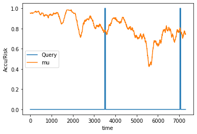
(b) MLDemon & PQ (same behavior). Both query for $2$ batches at empirical risk $R=516.2$.

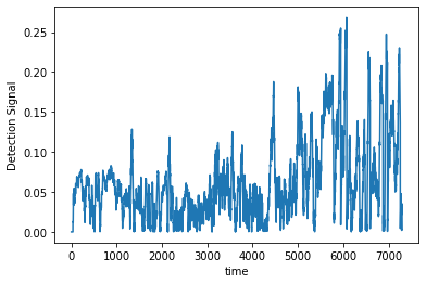
(c) Detection signal $G_{t}$

Figure 3: Sequential behavior on a single random seed for SPAM-CORPUS

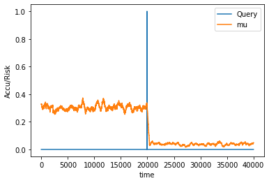
(a) RR at $\phi=5$.

(b) RR at $\phi=3$.

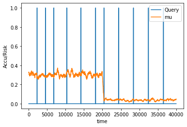
(c) MLD at $\alpha=64$.

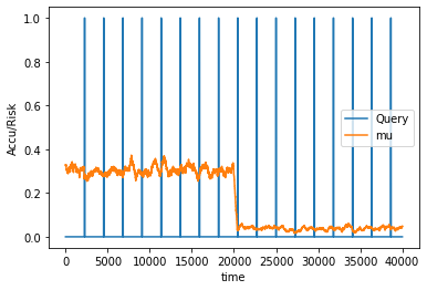
(d) PQ at $\alpha=64$.

(e) Detection signal $G_{t}$

Figure 4: Sequential behavior on a single random seed for FACE-RECOG

Interestingly, we can see that this example also illustrates an instance in which MLDemon and PQ behave the same. MLDemon needs at least a few samples in order to gain enough confidence in the model fit to extend the period. In the limit of few queries, MLDemon always performs like PQ.

In Fig. 4, all 3 policies attain roughly the same empirical risk. This is fairly intuitive from seeing when the query batches take place. However, we can see that the different policies use vastly different numbers of query batches to get here.

Compare 4a and 4b to see how RR picks the optimal time to query when only using 1 batch, but neglects the beginning of the stream as $\phi$ increases (resulting in label waste). This happens because the detection signal (4e) correctly detects the large drop in accuracy, but has a higher baseline after the drop than before.

Furthermore, observe how PQ uses 17 query batches in 4d while MLDemon uses only 11 in 4c. Furthermore, if we look closely at 4c, we can observe the way that MLDemon extends the query period after the first few batches, but reverts back when the detection signal spikes. This visualization neatly showcases MLDemon's behavior and how MLDemon builds an advantage over PQ.

References

- Abu-Mostafa et al., (2012) Abu-Mostafa, Y. S., Magdon-Ismail, M., and Lin, H.-T. (2012). Learning from data, volume 4. AMLBook New York, NY, USA:.
- Buteikis, (2019) Buteikis, A. (2019). Practical econometrics and data science.
- Cesa-Bianchi et al., (1997) Cesa-Bianchi, N., Freund, Y., Haussler, D., Helmbold, D. P., Schapire, R. E., and Warmuth, M. K. (1997). How to use expert advice. Journal of the ACM (JACM), 44(3):427–485.
- Chen et al., (2020) Chen, L., Zaharia, M., and Zou, J. (2020). Frugalml: How to use ml prediction apis more accurately and cheaply. arXiv preprint arXiv:2006.07512.
- Chen et al., (2019) Chen, Y., Xiong, J., Xu, W., and Zuo, J. (2019). A novel online incremental and decremental learning algorithm based on variable support vector machine. Cluster Computing, 22(3):7435–7445.
- Chen and Liu, (2018) Chen, Z. and Liu, B. (2018). Lifelong machine learning. Synthesis Lectures on Artificial Intelligence and Machine Learning, 12(3):1–207.
- Dorf et al., (1962) Dorf, R., Farren, M., and Phillips, C. (1962). Adaptive sampling frequency for sampled-data control systems. IRE Transactions on Automatic Control, 7(1):38–47.
- Duchi, (2016) Duchi, J. (2016). Lecture notes for statistics 311/electrical engineering 377. URL: https://stanford. edu/class/stats311/Lectures/full_notes. pdf. Last visited on, 2:23.
- Farias and Megiddo, (2006) Farias, D. P. D. and Megiddo, N. (2006). Combining expert advice in reactive environments. Journal of the ACM (JACM), 53(5):762–799.
- Feizi et al., (2010) Feizi, S., Goyal, V. K., and Médard, M. (2010). Locally adaptive sampling. In 2010 48th Annual Allerton Conference on Communication, Control, and Computing (Allerton), pages 152–159. IEEE.
- Fern and Givan, (2003) Fern, A. and Givan, R. (2003). Online ensemble learning: An empirical study. Machine Learning, 53(1):71–109.
- Fontenla-Romero et al., (2013) Fontenla-Romero, Ó., Guijarro-Berdiñas, B., Martinez-Rego, D., Pérez-Sánchez, B., and Peteiro-Barral, D. (2013). Online machine learning. In Efficiency and Scalability Methods for Computational Intellect, pages 27–54. IGI Global.
- Garg et al., (2020) Garg, S., Wu, Y., Balakrishnan, S., and Lipton, Z. C. (2020). A unified view of label shift estimation. arXiv preprint arXiv:2003.07554.
- Gomes et al., (2019) Gomes, H. M., Read, J., Bifet, A., Barddal, J. P., and Gama, J. (2019). Machine learning for streaming data: state of the art, challenges, and opportunities. ACM SIGKDD Explorations Newsletter, 21(2):6–22.
- Goodfellow et al., (2018) Goodfellow, I., McDaniel, P., and Papernot, N. (2018). Making machine learning robust against adversarial inputs. Communications of the ACM, 61(7):56–66.
- Hayes and Kanan, (2020) Hayes, T. L. and Kanan, C. (2020). Lifelong machine learning with deep streaming linear discriminant analysis. In Proceedings of the IEEE/CVF Conference on Computer Vision and Pattern Recognition Workshops, pages 220–221.
- He et al., (2015) He, K., Zhang, X., Ren, S., and Sun, J. (2015). Deep residual learning for image recognition. arxiv 2015. arXiv preprint arXiv:1512.03385.
- Hoeffding, (1994) Hoeffding, W. (1994). Probability inequalities for sums of bounded random variables. In The Collected Works of Wassily Hoeffding, pages 409–426. Springer.
- Hoi et al., (2014) Hoi, S. C., Wang, J., and Zhao, P. (2014). Libol: A library for online learning algorithms. Journal of Machine Learning Research, 15(1):495.
- Hong et al., (2018) Hong, X., Wong, P., Liu, D., Guan, S.-U., Man, K. L., and Huang, X. (2018). Lifelong machine learning: outlook and direction. In Proceedings of the 2nd International Conference on Big Data Research, pages 76–79.
- Johnson et al., (2000) Johnson, R. A., Miller, I., and Freund, J. E. (2000). Probability and statistics for engineers, volume 2000. Pearson Education London.
- Karp, (1992) Karp, R. M. (1992). On-line algorithms versus off-line algorithms: How much. In Algorithms, Software, Architecture: Information Processing 92: Proceedings of the IFIP 12th World Computer Congress, Madrid, Spain, 7-11 September 1992, volume 1, page 416. North-Holland.
- Katakis et al., (2006) Katakis, I., Tsoumakas, G., and Vlahavas, I. (2006). Dynamic feature space and incremental feature selection for the classification of textual data streams. in in ecml/pkdd-2006 international workshop on knowledge discovery from data streams.
- Kulinski et al., (2020) Kulinski, S., Bagchi, S., and Inouye, D. I. (2020). Feature shift detection: Localizing which features have shifted via conditional distribution tests. Advances in Neural Information Processing Systems, 33.
- Le Cam, (2012) Le Cam, L. (2012). Asymptotic methods in statistical decision theory. Springer Science & Business Media.
- Lecué et al., (2020) Lecué, G., Lerasle, M., et al. (2020). Robust machine learning by median-of-means: theory and practice. Annals of Statistics, 48(2):906–931.
- Li, (2018) Li, J. Z. (2018). Principled approaches to robust machine learning and beyond. PhD thesis, Massachusetts Institute of Technology.
- Lilliefors, (1967) Lilliefors, H. W. (1967). On the kolmogorov-smirnov test for normality with mean and variance unknown. Journal of the American statistical Association, 62(318):399–402.
- Lipton et al., (2018) Lipton, Z., Wang, Y.-X., and Smola, A. (2018). Detecting and correcting for label shift with black box predictors. In International conference on machine learning, pages 3122–3130. PMLR.
- Liu, (2017) Liu, B. (2017). Lifelong machine learning: a paradigm for continuous learning. Frontiers of Computer Science, 11(3):359–361.
- Lu et al., (2018) Lu, J., Liu, A., Dong, F., Gu, F., Gama, J., and Zhang, G. (2018). Learning under concept drift: A review. IEEE Transactions on Knowledge and Data Engineering, 31(12):2346–2363.
- Luenberger et al., (1984) Luenberger, D. G., Ye, Y., et al. (1984). Linear and nonlinear programming, volume 2. Springer.
- Mahmud, (1989) Mahmud, S. M. (1989). High precision phase measurement using adaptive sampling. IEEE Transactions on Instrumentation and Measurement, 38(5):954–960.
- Miller et al., (2020) Miller, J., Krauth, K., Recht, B., and Schmidt, L. (2020). The effect of natural distribution shift on question answering models. In International Conference on Machine Learning, pages 6905–6916. PMLR.
- Minku et al., (2009) Minku, L. L., White, A. P., and Yao, X. (2009). The impact of diversity on online ensemble learning in the presence of concept drift. IEEE Transactions on knowledge and Data Engineering, 22(5):730–742.
- Montgomery et al., (2009) Montgomery, D. C., Runger, G. C., and Hubele, N. F. (2009). Engineering statistics. John Wiley & Sons.
- Morris, (1977) Morris, P. A. (1977). Combining expert judgments: A bayesian approach. Management Science, 23(7):679–693.
- Munro and Paterson, (1980) Munro, J. I. and Paterson, M. S. (1980). Selection and sorting with limited storage. Theoretical computer science, 12(3):315–323.
- Naaman, (2021) Naaman, M. (2021). On the tight constant in the multivariate dvoretzky–kiefer–wolfowitz inequality. Statistics & Probability Letters, 173:109088.
- Nagabandi et al., (2018) Nagabandi, A., Finn, C., and Levine, S. (2018). Deep online learning via meta-learning: Continual adaptation for model-based rl. arXiv preprint arXiv:1812.07671.
- Nallaperuma et al., (2019) Nallaperuma, D., Nawaratne, R., Bandaragoda, T., Adikari, A., Nguyen, S., Kempitiya, T., De Silva, D., Alahakoon, D., and Pothuhera, D. (2019). Online incremental machine learning platform for big data-driven smart traffic management. IEEE Transactions on Intelligent Transportation Systems, 20(12):4679–4690.
- O'Searcoid, (2006) O'Searcoid, M. (2006). Metric spaces. Springer Science & Business Media.
- Pedregosa et al., (2011) Pedregosa, F., Varoquaux, G., Gramfort, A., Michel, V., Thirion, B., Grisel, O., Blondel, M., Prettenhofer, P., Weiss, R., Dubourg, V., et al. (2011). Scikit-learn: Machine learning in python. the Journal of machine Learning research, 12:2825–2830.
- Peng and Nair, (2009) Peng, J.-H. and Nair, N.-K. (2009). Adaptive sampling scheme for monitoring oscillations using prony analysis. IET generation, transmission & distribution, 3(12):1052–1060.
- Pinto et al., (2019) Pinto, F., Sampaio, M. O., and Bizarro, P. (2019). Automatic model monitoring for data streams. arXiv preprint arXiv:1908.04240.
- Polikar, (2012) Polikar, R. (2012). Ensemble learning. In Ensemble machine learning, pages 1–34. Springer.
- Rabanser et al., (2018) Rabanser, S., Günnemann, S., and Lipton, Z. C. (2018). Failing loudly: An empirical study of methods for detecting dataset shift. arXiv preprint arXiv:1810.11953.
- Schelter et al., (2020) Schelter, S., Rukat, T., and Biessmann, F. (2020). Learning to validate the predictions of black box classifiers on unseen data. In Proceedings of the 2020 ACM SIGMOD International Conference on Management of Data, pages 1289–1299.
- Shafique et al., (2020) Shafique, M., Naseer, M., Theocharides, T., Kyrkou, C., Mutlu, O., Orosa, L., and Choi, J. (2020). Robust machine learning systems: Challenges, current trends, perspectives, and the road ahead. IEEE Design & Test, 37(2):30–57.
- Shao et al., (2020) Shao, Z., Yang, J., and Ren, S. (2020). Increasing trustworthiness of deep neural networks via accuracy monitoring. arXiv preprint arXiv:2007.01472.
- Sutherland, (2009) Sutherland, W. A. (2009). Introduction to metric and topological spaces. Oxford University Press.
- Szpankowski, (2011) Szpankowski, W. (2011). Average case analysis of algorithms on sequences, volume 50. John Wiley & Sons.
- Tipping, (2003) Tipping, M. E. (2003). Bayesian inference: An introduction to principles and practice in machine learning. In Summer School on Machine Learning, pages 41–62. Springer.
- Valluri et al., (2000) Valluri, S. R., Jeffrey, D. J., and Corless, R. M. (2000). Some applications of the lambert w function to physics. Canadian Journal of Physics, 78(9):823–831.
- Veberič, (2012) Veberič, D. (2012). Lambert w function for applications in physics. Computer Physics Communications, 183(12):2622–2628.
- Villani, (2008) Villani, C. (2008). Optimal transport: old and new, volume 338. Springer Science & Business Media.
- Wang et al., (2019) Wang, X., Kang, Q., An, J., and Zhou, M. (2019). Drifted twitter spam classification using multiscale detection test on kl divergence. IEEE Access, 7:108384–108394.
- Wang et al., (2020) Wang, Z., Wang, G., Huang, B., Xiong, Z., Hong, Q., Wu, H., Yi, P., Jiang, K., Wang, N., Pei, Y., et al. (2020). Masked face recognition dataset and application. arXiv preprint arXiv:2003.09093.
- Xuan et al., (2020) Xuan, J., Lu, J., and Zhang, G. (2020). Bayesian nonparametric unsupervised concept drift detection for data stream mining. ACM Transactions on Intelligent Systems and Technology (TIST), 12(1):1–22.
- Yu, (1997) Yu, B. (1997). Assouad, fano, and le cam. In Festschrift for Lucien Le Cam, pages 423–435. Springer.
- Yu et al., (2018) Yu, S., Wang, X., and Príncipe, J. C. (2018). Request-and-reverify: hierarchical hypothesis testing for concept drift detection with expensive labels. In Proceedings of the 27th International Joint Conference on Artificial Intelligence, pages 3033–3039.
- Zhang et al., (2019) Zhang, J. J., Liu, K., Khalid, F., Hanif, M. A., Rehman, S., Theocharides, T., Artussi, A., Shafique, M., and Garg, S. (2019). Building robust machine learning systems: Current progress, research challenges, and opportunities. In Proceedings of the 56th Annual Design Automation Conference 2019, pages 1–4.
- Zhao et al., (2019) Zhao, H., Des Combes, R. T., Zhang, K., and Gordon, G. (2019). On learning invariant representations for domain adaptation. In International Conference on Machine Learning, pages 7523–7532. PMLR.