Noise driven current reversal and stabilisation in the tilted ratchet potential subject to tempered stable Lévy noise

Abstract

We consider motion of a particle in a one-dimensional tilted ratchet potential subject to two-sided tempered stable Lévy noise characterised by strength $\Omega$, fractional index $\alpha$, skew $\theta$ and tempering $\lambda$. We derive analytic solutions to the corresponding Fokker-Planck Lévy equations for the probability density. Due to the periodicity of the potential, we carry out reduction to a compact domain and solve for the analogue there of steady-state solutions which we represent as wrapped probability density functions. By solving for the expected value of the current associated with the particle motion, we are able to determine threshold for metastability of the system, namely when the particle stabilises in a well of the potential and when the particle is in motion, for example as a consequence of the tilt of the potential. Because the noise may be asymmetric, we examine the relationship between skew of the noise and the tilt of the potential. With tempering, we find two remarkable regimes where the current may be reversed in a direction opposite to the tilt or where the particle may be stabilised in a well in circumstances where deterministically it should flow with the tilt.

Keywords: Fokker-Planck, tempered-stable Lévy noise, tilted ratchet potential

I Introduction

The impact of stochastic driving in non-linear systems Reimann02 is significant in diverse physical, chemical, and biological systems; we would also include here social systems for reasons to be given soon. For all the sophistication of many models here, some features are common: a potential energy landscape with a tilt - or bias - superimposed with some form of periodicity in the distributions of local minima. These are known as tilted ratchet potentials because of the behaviour that, under metastable circumstances, a particle may drift down the tilt but temporarily ‘catch’ in the periodically occuring wells Linder01 . Many works have addressed Gaussian or Brownian noise in such potentials, or analogous forms such as ‘washboard’ potentials Henn2009 ; MulHenn2011 , and multi-dimensional forms of these ChallJack2013 . However, more general forms of noise particularly with jumps drawn from heavy-tails BorovkovBorovkov08 are now topical in the literature, for example spatially stable Lévy noise Chambers76 ; Twee1984 and tempered stable Lévy noise MantStan1994 ; Koponen1995 ; BaeMeer2010 ; GajMag2010 ; MeerSab2016 - leading to the study of so-called fractional (or super) diffusion MetzKlaft2000 ; Jumarie2004 ; MetzKlaft2004 . There is a long history of applications to more standard one-dimensional systems JMF1999 ; MetzKlaft2000b ; CGKMT2002 ; MagWer2007 ; CGGKS2008 ; Gorska2011 . Such non-Gaussian noise models have been applied to ratchet potentials in the absence of tilt KullCast2012 . In this paper we extend these analyses to the case of non-zero tilt.

The signature behaviours of interest in stochastic tilted ratchets RPHR2002 ; Henn2009 ; MulHenn2011 are those of current stabilisation - where the particle may be localised in a well under the influence of the noise when deterministically it would seek to roll down the tilt - and current reversal - where the particle is driven against the tilt by the noise. This phenomena form a subset of non-linear collective behaviours alongside stochastically driven resonance GHJM1998 ; GHJM2009 and synchronisation Kawa2014 . Given the importance of noise characterised by jumps and heavy tails in diverse contexts Kleinert2009 such as the fluid properties of plasmas delCastCarrLyn2005 ; delCastGonCheck2008 , finance EllvdHoek2003 ; CarteaDelCast2007 and brain waves RobBoonBreak2015 , the application of this to the collective phenomena of tilted ratchets is evident. Already in the presence of periodic potentials under tempered stable noise, current reversal has been observed KullCast2012 . In this paper we explore the role in this phenomenon of the tilt - which should naturally inhibit current reversal - in the vicinity of the deterministic threshold for current flow.

Our interest in this problem arises from a quite different problem, that of synchronisation on networks as exemplified in the stylised Kuramoto model Kur84 . Firstly, the property of metastability for the Kuramoto model on ring graphs subject to weak Gaussian noise has been identified DeVille12 . This uses the approach to stochastic metastability of Freidlin-Wentzell (FW) theory Freidlin98 . Secondly, the Kuramoto model close to the synchronisation threshold maps to a tilted ratchet potential; some of us have explored this property for a generalisation of the Kuramoto model for two populations on separate networks ZupKall2013 and subject to Gaussian noise Holder2017 . Finally, some of us have begun explorations of the ordinary Kuramoto model subject to stable KallRob2017 and tempered stable noise KallRob2017b - with hints at stochastic synchronisation there as well.

The paper is structured as follows. In the next section we set-up the tempered stable stochastic system, first using the fractional Langevin formalism and then the Fokker-Planck formalism. We then discuss the reduction procedure in light of the periodic structure of the potential, using the Gaussian case as an example. We then present the main results showing the solution to the reduced Fokker-Planck probability density and associated expected value of the current associated with the particle; in this we use a little-known representation of the solutions as ‘wrapped probability densities’. We examine these under variations of parameters such as the fractional $\alpha$, the tilt and the tempering of the noise. Here we identify the regimes of current reversal and stabilisation. The paper concludes with prospects for future work.

II Tempered-fractional-Fokker-Planck equations

II.1 Fractional Langevin equations

We begin with a generalisation of the Langevin equation capturing the combination of deterministic and stochastic dynamics written in stochastic differential notation:

$$dx(t)=-V^{\prime}(x(t))dt+dL^{\alpha,\theta,\lambda}(t)$$ (1)

where $\alpha\in(0,1)\cup(1,2]$ is the fractional index describing the power law behaviour of the Lévy process, $\theta\in[-1,1]$ is the asymmetry or skew of the noise distribution, and $\lambda\in(0,\infty)$ is the tempering parameter for the heavy tails KawMas2011 . For $\alpha=2$, the Lévy noise term in Eq.(1) becomes Gaussian.

For this work the potential $V(x)$ is given by

$$V(x)=-\mu x-\gamma\cos(x-\rho),\;\;\rho\in(-\pi,\pi]$$ (2)

where $\mu\in\mathbb{R}$ and $\gamma\in\mathbb{R}$ are referred to as the tilt and amplitude respectively. Eq.(2) is commonly referred to as a tilted periodic ratchet Linder01 ; Reimann02 . The potential has two important features. The first is the periodicity $V^{\prime}(x)=V^{\prime}(x+2\pi)$. The second is given by the sign of the quantity

$${\cal K}=\gamma^{2}-\mu^{2}$$ (3)

which encapsulates the interplay between the tilt and the amplitude. Specifically, if ${\cal K}>0$ then $V(x)$ contains a series of local minima (stable fixed points) at $x=\rho+\sin^{-1}(\mu/\gamma)$ mod $2\pi$, and a series of local maxima (unstable fixed points) at $x=\pi+\rho-\sin^{-1}(\mu/\gamma)$ mod $2\pi$. If ${\cal K}=0$ then the maxima and minima collapse into each other and form a series of inflection points (unstable fixed points). Lastly, if ${\cal K}<0$ then $V(x)$ becomes an entirely monotonic function with no inflection points, namely no stationary points.

II.2 Tempered-fractional diffusion

The probability density ${\cal P}(x,t)$ associated with the tempered-stable Lévy process in Eq.(1) obeys the following so-called Tempered Fractional Fokker-Planck equation (TFFP) Cartea07

$$\begin{split}\frac{\partial}{\partial t}{\cal P}(x,t)=\left\{\Omega\partial^{\alpha,\theta,\lambda}_{x}+\frac{\partial}{\partial x}V^{\prime}(x)\right\}{\cal P}(x,t)\\ {\cal P}(x,0)=\delta(x-y),\end{split}$$ (4)

where $\Omega\in\mathbb{R}_{+}$ is the diffusivity and the operator $\partial^{\alpha,\theta,\lambda}_{x}$ is the tempered-fractional-diffusion operator, given explicitly by KullCast2012

$$\partial^{\alpha,\theta,\lambda}_{x}={\cal D}^{\alpha,\theta,\lambda}_{x}+v^{\alpha,\theta,\lambda}\frac{\partial}{\partial x}+\nu^{\alpha,\lambda}.$$ (5)

Here $v^{\alpha,\theta,\lambda}$ and $\nu^{\alpha,\lambda}$ are so-called ‘induced’ drift and source/sink terms given by,

$$v^{\alpha,\theta,\lambda}=\left\{\begin{array}[]{cl}0,&\alpha\in(0,1)\\ \frac{\alpha\theta\lambda^{\alpha-1}}{|\cos(\pi\alpha/2)|}&\alpha\in(1,2)\end{array}\right.,\;\;\nu^{\alpha,\lambda}=\frac{\lambda^{\alpha}}{\cos(\pi\alpha/2)}.$$ (6)

The operator ${\cal D}^{\alpha,\theta,\lambda}_{x}$ is the $\lambda$-truncated fractional derivative of order $\alpha$, given by,

$${\cal D}^{\alpha,\theta,\lambda}_{x}=l(\theta)e^{-\lambda x}\,_{-\infty}D^{\alpha}_{x}e^{\lambda x}-r(\theta)e^{\lambda x}\,_{x}D^{\alpha}_{\infty}e^{-\lambda x}$$ (7)

where the operators $\,{}_{-\infty}D^{\alpha}_{x}$ and $\,{}_{x}D^{\alpha}_{\infty}$ are the Riemann-Liouville derivatives del-Castillo-Negrete12 . Both operators have the following form in Fourier space Podlubny99 ; Samko93

$$\begin{split}{\cal F}\left[e^{-\lambda x}\,_{-\infty}D^{\alpha}_{x}e^{\lambda x}f(x)\right]=(\lambda-ik)^{\alpha}\widehat{f}(k)\\ {\cal F}\left[e^{\lambda x}\,_{x}D^{\alpha}_{\infty}e^{-\lambda x}f(x)\right]=(\lambda+ik)^{\alpha}\widehat{f}(k)\end{split}$$ (8)

where our convention for the Fourier transform is:

$$\begin{split}{\cal F}\left[f(x)\right]=\int^{\infty}_{-\infty}dxe^{ikx}f(x)=\widehat{f}(k)\\ {\cal F}^{-1}\left[\widehat{f}(k)\right]=\int^{\infty}_{-\infty}\frac{dk}{2\pi}e^{-ikx}\widehat{f}(k)=f(x).\end{split}$$ (9)

Finally, for definitional purposes, the weighting factors

$$l(\theta)=\frac{\theta-1}{2\cos(\pi\alpha/2)},\;\;r(\theta)=\frac{\theta+1}{2\cos(\pi\alpha/2)}$$ (10)

give the asymmetry imposed on each of the Riemann-Liouville derivatives. Taking the Fourier transform of the fractional derivative $\partial^{\alpha,\theta,\lambda}_{x}$ we obtain

$$\begin{split}{\cal F}\left[\partial^{\alpha,\theta,\lambda}_{x}f(x)\right]=\left\{l(\theta)(\lambda-ik)^{\alpha}\right.\\ \left.-r(\theta)(\lambda+ik)^{\alpha}-ikv^{\alpha,\theta,\lambda}+\nu^{\alpha,\lambda}\right\}\widehat{f}(k)\\ =\Lambda(k)\widehat{f}(k)\end{split}$$ (11)

where $\Lambda(k)$ is the logarithm of the characteristic function of the tempered stable Lévy process. For example, the limit $\lambda\rightarrow 0$ reproduces the Lévy-Khinchine law for the stable process Sato99 .

II.3 Illustrative example - Gaussian limit

In order to proceed with the general TFFP equation with the tilted ratchet potential, we first briefly detail the Gaussian limit case, namely

$$\frac{\partial}{\partial t}{\cal P}(x,t)=\left\{\Omega\frac{\partial^{2}}{\partial x^{2}}+\frac{\partial}{\partial x}V^{\prime}(x)\right\}{\cal P}(x,t)$$ (12)

as its relatively simple explanation of solution allows for greater intuition when we consider the more complicated fractional case. As well as the defining equation, Eq. (12), we are also concerned with the probability current ${\cal J}(x,t)$, defined by the following probability conservation expression

$$\begin{split}&&\frac{\partial}{\partial t}{\cal P}(x,t)+\frac{\partial}{\partial x}{\cal J}(x,t)=0\\ \Rightarrow&&{\cal J}(x,t)=-\left\{\Omega\frac{\partial}{\partial x}+V^{\prime}(x)\right\}{\cal P}(x,t).\end{split}$$ (13)

As explained in Reimann02 and references therein, one finds a non-normalisable density when following the usual procedure for a steady-state solution: solving the Pearson equation for the steady state density ${\cal P}_{st}(x)$, namely setting $\frac{\partial}{\partial t}{\cal P}(x,t)=0$ in Eq.(12), and applying the vanishing boundary condition ${\cal P}_{st}(x)\rightarrow 0$ at the natural boundaries $x\rightarrow\pm\infty$. This is due to the periodicity of the ratchet potential and its metastability in the presence of noise Freidlin98 ; Berglund07 ; DeVille12 . In order to circumvent this phenomenon, we restrict the support of $x$ to $\mathbb{S}^{1}$ by constructing the so-called reduced density ${\cal P}^{(r)}(x,t)$ and reduced probability current ${\cal J}^{(r)}(x,t)$ through

$$\begin{split}{\cal P}^{(r)}(x,t)\equiv\sum^{\infty}_{n=-\infty}{\cal P}(x+2\pi n,t),\\ {\cal J}^{(r)}(x,t)\equiv\sum^{\infty}_{n=-\infty}{\cal J}(x+2\pi n,t).\end{split}$$ (14)

Due to the linearity of the Fokker-Planck equation, the reduced density and reduced probability current also obey Eqs.(12) and (13) respectively, but with the new boundary and normalisation conditions

$${\cal P}^{(r)}(-\pi,t)={\cal P}^{(r)}(\pi,t),\;\;\int^{\pi}_{-\pi}dx{\cal P}^{(r)}(x,t)=1.$$ (15)

The reduced steady state density is then given by Stratonovich67

$${\cal P}_{st}^{(r)}(x)=\frac{\sinh\left(\frac{\pi\mu}{\Omega}\right)e^{-\frac{V(x)}{\Omega}}\int^{x+2\pi}_{x}d\varphi e^{\frac{V(\varphi)}{\Omega}}}{2\pi^{2}\left|I_{i\mu}\left(\frac{\gamma}{\Omega}\right)\right|^{2}\left(1-e^{-\frac{2\pi\mu}{\Omega}}\right)}$$ (16)

where $I_{i\mu}$ is the modified Bessel function of imaginary order.

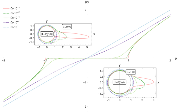
Figure 1: Examples of Eq.(16) (insets) and Eq.(17) (main) for $\rho=-1.5$ and $\gamma=1$ and various values of the diffusivity $\Omega$ which governs noise strength. The leftmost inset details a case with stable fixed points in the potential ($\mu=0.99$), the rightmost inset details a case with no fixed points in the potential ($\mu=1.01$). Both insets are given as a parametric plot governed by Eq.(18).

Additionally, the corresponding average velocity $\langle\dot{x}\rangle$, which may assume non-zero values as a consequence of the metastability and the tilt of the potential $\mu$, is given by Stratonovich67

$$\langle\dot{x}\rangle=\frac{d}{dt}\langle x\rangle=\int^{\pi}_{-\pi}dx{\cal J}^{(r)}_{st}(x)=\frac{\Omega\sinh\left(\frac{\pi\mu}{\Omega}\right)}{\pi\left|I_{i\mu}\left(\frac{\gamma}{\Omega}\right)\right|^{2}}.$$ (17)

Note that, trivially, for Gaussian noise there is zero average velocity in the absence of tilt: $\langle\dot{x}\rangle=0$ if $\mu=0$.

Fig.1 gives examples of Eq.(16) (insets) and Eq.(17) (main figure) where we have fixed the amplitude $\gamma=1$; thus deterministically, the point of instability ${\cal K}=0$ occurs when $\mu=\pm 1$ from Eq.(3) so for $\mu=(-1,1)$ $\dot{x}(t\rightarrow\infty)=0$. We also choose the offset $\rho=-1.5$. The main part of Fig. 1 shows the average velocity $\langle\dot{x}\rangle$ as a function of the tilt $\mu$. We see that for weak noise, $\Omega=10^{-3}$, the current is vanishing inside the interval $(-1,1)$ and increases positively, respectively negatively, for $\mu>1$, respectively $<-1$. The particle ‘rolls’ in the direction of the tilt. For increasing $\Omega$ in the Gaussian noise, the current assumes non-zero values inside the region where deterministically it should vanish: the noise generates tails that allow the particle to ‘spill’ outside the potential wells giving a non-vanishing probability that the particle rolls with the tilt when deterministically it should be stable; hence the particle is metastable.

We also examine these same properties through the probability density solutions of the Gaussian Fokker-Planck equation as insets in Fig.1. The left-most inset provides a case with stable fixed points ($\gamma=1$, $\mu=0.99$) and the right-most inset details a case with no fixed points ($\gamma=1$, $\mu=1.01$). Both insets are presented as so-called ‘wrapped probability density functions’ (see for example Fish96 ), namely a parametric plot where

$$\{x,y\} = \left\{\left(1+{\cal P}_{st}^{(r)}(\phi)\right)\cos\phi,\left(1+{\cal P}_{st}^{(r)}(\phi)\right)\sin\phi\right\},$$ (18)

$$\textrm{for }\;\;\phi\in\mathbb{S}^{1}.$$

Note that in such plots the convention is that the positive horizontal axis represents $\phi=0$ (which would correspond to the vertical axis for a density on the real line), peaks located clockwise from this are in the positive direction and those anti-clockwise are in the negative.

For the leftmost inset in Fig.1, for small $\Omega$ we see that the density is approximately concentrated at the deterministic position of the stable fixed point ($\phi=\rho+\sin^{-1}(\mu/\gamma)\approx-0.07$, and thus the peak is oriented slightly below the horizontal axis). Moreover, as $\Omega$ increases we see that the probability density begins to smear around the circle, losing any discernable features after $\Omega=1$. This displays the phenomenon of metastability in the wrapped densities: the particle is rolling with some probability so the probability density is distributed around the entire circle.

The narrative is similar for the right-most inset, except the relative heights of the densities is significantly less - indicating that even for the weakest noise there is non-vanishing probability that the particle is at other points around the circle because deterministically the particle will roll for $\mu>1$. Further increases in $\Omega$ distends the peak until it is uniformly distributed around the circle.

The wrapped densities also provide insight into the range of fluctuations. So, for $\mu=1.01$ the weakest noise $\Omega=10^{-3}$ has a density that is evenly distributed on either side of the horizontal axis, indicating that fluctuations about the average of zero are symmetrically distributed. As $\Omega$ increases, the bulge moves clock-wise around from the horizontal axis indicating that fluctuations are biased in the positive direction - the direction of the tilt. Similar properties are seen for $\mu=0.99$ but at stronger values of $\Omega$.

III Analytic solution of the TFFP equation

III.1 Reduced density

As with the Gaussian case, we expect that the steady state equivalent of Eq.(4) with vanishing boundary conditions at the natural boundaries $x\rightarrow\pm\infty$ will be non-normalisable due to metastability. In order to ameliorate this situation we again consider a reduced density defined on $\mathbb{S}^{1}$ (Eq.(14)) for the steady state TFFP equation

$$\left\{\Omega\partial^{\alpha,\theta,\lambda}_{x}+\frac{\partial}{\partial x}V^{\prime}(x)\right\}{\cal P}^{(r)}_{st}(x)=0$$ (19)

with boundary and normalisation conditions given by Eq.(15).

Taking the Fourier transform of Eq.(19) we obtain

$$\begin{split}&\left\{\Omega\Lambda(k)+ik\mu\right\}{\widehat{\cal P}}^{(r)}_{st}(k)\\ &=\frac{k\gamma}{2}\left\{e^{-i\rho}{\widehat{\cal P}}^{(r)}_{st}(k+1)-e^{i\rho}{\widehat{\cal P}}^{(r)}_{st}(k-1)\right\}\\ \Rightarrow&\;\;\widehat{Q}(k+1)=-f_{k}\widehat{Q}(k)+\widehat{Q}(k-1),\end{split}$$ (20)

where $\widehat{Q}(k)=e^{-ik\rho}{\widehat{\cal P}}^{(r)}_{st}(k)$ and

$$f_{k}=-\frac{2}{k\gamma}\left\{\Omega\Lambda(k)+ik\mu\right\}.$$ (21)

Eq.(20) represents a linear three-term recurrence relation defining the coefficients in the Fourier expansion.

Because of the periodic boundary conditions of ${\cal P}^{(r)}_{st}(x)$ on the finite interval, the Fourier variable $k$ only takes discrete values. Specifically,

$${\cal F}\left[{\cal P}^{(r)}_{st}(x)\right]=\sum^{\infty}_{n=-\infty}{\cal F}\left[{\cal P}_{st}(x+2\pi n)\right]$$

$$=\widehat{{\cal P}}_{st}(k)\sum^{\infty}_{n=-\infty}e^{-i2\pi nk}$$

$$=\widehat{{\cal P}}_{st}(k)\sum^{\infty}_{m=-\infty}\delta(k-m).$$

Thus we need to solve the three term recurrence relation for coefficients $\widehat{Q}(k)$ in Eq.(20) for $k\in\{\dots,-1,0,1,\dots\}$. Doing so, we can then construct the probability density via the discrete inverse Fourier transform

$${\cal P}^{(r)}_{st}(x)=\frac{1}{2\pi}\left\{\widehat{Q}(0)+2\Re\sum^{\infty}_{n=1}e^{-in(x-\rho)}\widehat{Q}(n)\right\}$$ (22)

where $\widehat{Q}(0)=1$ from the normalisation condition in Eq.(15).

Following Chap.9 of Risken89 , applying the transformations

$$S_{k+1}=\frac{\widehat{Q}(k+1)}{\widehat{Q}(k)}$$

the linear three term recurrence relation in Eq.(20) becomes the following non-linear two term recurrence relation

$$S_{k}=\frac{1}{f_{k}+S_{k+1}}$$ (23)

which can be solved iteratively using continued fractions

$$S_{k}=\cfrac{1}{f_{k}+\cfrac{1}{f_{k+1}+S_{k+2}}}=\cfrac{1}{f_{k}+\cfrac{1}{f_{k+1}+\cfrac{1}{f_{k+2}+\cfrac{1}{\ddots}}}}$$

Moreover, applying the notation

$$\mathbb{K}^{m}_{j=1}(a_{j}:b_{j})=\cfrac{a_{1}}{b_{1}+\cfrac{a_{2}}{b_{2}+\cfrac{a_{3}}{\dots+\cfrac{a_{m}}{b_{m}}}}}$$

$S_{k}$ can be conveniently expressed by

$$S_{k}=\mathbb{K}^{\infty}_{j=k}(1:f_{k}).$$ (24)

Calculating the expressions for $\{S_{k},S_{k-1},\dots,S_{2},S_{1}\}$, we may then reconstruct the corresponding $\widehat{Q}(k)$ using

$$\widehat{Q}(k)=S_{k}S_{k-1}\dots S_{2}S_{1}\widehat{Q}(0)$$ (25)

for insertion into Eq.(22). Thus Eq.(22) with coefficients given by Eq.(25) is the solution to the TFFP equation, equivalent to Eq.(16) for Gaussian noise.

For numerical calculations of the reduced density we truncate the number of terms in Eq.(22) to $n=\{1,\dots,1000\}$. Moreover, for the continued fractions $S_{k}$ in Eq.(24) that form the density in Eq.(22), we approximate these as $S_{k}=\mathbb{K}^{p}_{j=k}(1:f_{k})$, where $k=\{1,\dots,1000\}$, and $p=2000$.

III.2 Average velocity

Considering the expression for the the average velocity $\langle\dot{x}\rangle\equiv\frac{d}{dt}\langle x\rangle$ given in Eq.(17) we may perform the following sequence of manipulations to re-express the expected current in terms of the characteristic function for the tempered stable Lévy process:

$$\frac{d}{dt}\langle x\rangle = \frac{d}{dt}\langle xe^{ikx}\rangle|_{k\rightarrow 0}$$

$$= \frac{\partial}{\partial t}\left\{-i\frac{\partial}{\partial k}\widehat{{\cal P}}(k,t)\right\}|_{k\rightarrow 0}$$

$$= -i\frac{\partial}{\partial k}\left\{\frac{\partial}{\partial t}\widehat{{\cal P}}(k,t)\right\}|_{k\rightarrow 0}$$

$$= -i\frac{\partial}{\partial k}\left\{\Omega\Lambda(k)\widehat{{\cal P}}(k,t)-ik{\cal F}\left[V^{\prime}(x){\cal P}(x,t)\right]\right\}|_{k\rightarrow 0}$$

$$= -i\Omega\frac{d}{dk}\Lambda(k)|_{k\rightarrow 0}-{\cal F}\left[V^{\prime}(x){\cal P}(x,t)\right]|_{k\rightarrow 0}.$$

From Eq.(11)

$$-i\Omega\frac{d}{dk}\Lambda(k)|_{k\rightarrow 0}=\left\{\begin{array}[]{cl}-\frac{\Omega\alpha\theta\lambda^{\alpha-1}}{\cos\left(\frac{\pi\alpha}{2}\right)}&0<\alpha<1\\ 0&1<\alpha<2\end{array}\right.$$

and from Eqs.(2) and (22)

$$-{\cal F}\left[V^{\prime}(x){\cal P}(x,t)\right]|_{k\rightarrow 0}=\mu-2\pi\gamma\Im\left\{\widehat{Q}(1)\right\}.$$

Hence the expected value of the velocity may be expressed as

$$\langle\dot{x}\rangle=\left\{\begin{array}[]{cl}-\frac{\Omega\alpha\theta\lambda^{\alpha-1}}{\cos\left(\frac{\pi\alpha}{2}\right)}+\mu-2\pi\gamma\Im\left\{\widehat{Q}(1)\right\}&0<\alpha<1\\ \mu-2\pi\gamma\Im\left\{\widehat{Q}(1)\right\}&1<\alpha<2.\end{array}\right.$$ (26)

Eq.(26) with $\widehat{Q}(1)$ given by Eq.(25) is the tempered-stable equivalent of Eq.(17) for Gaussian noise.

For the corresponding numerical calculations of the average velocity in Eq.(26), only the first continued fraction coefficient $\widehat{Q}(1)=S_{1}\widehat{Q}(0)$ is involved. For numerical purposes we again truncate $S_{1}$ as $S_{1}=\mathbb{K}^{p}_{j=1}(1:f_{k})$. For $\alpha>1$ we apply $p=2\times 10^{4}$. However, for $\alpha<1$ we have found it necessary to set $p=4\times 10^{4}$ to obtain sufficiently smooth plots of the average velocity.

IV Examples: Current stabilisation and reversal

As for the Gaussian case, we fix the amplitude $\gamma=1$ so that the deterministic threshold for instability is $\mu=\pm 1$. We also fix the diffusivity constant at $\Omega=0.1$, where the Gaussian case in Fig.1 shows diffusion even for $\mu<1$ due to metastability, and $\rho=-1.5$ as before. We first examine the average velocity and wrapped densities for selective values of $\alpha$ and $\lambda$.

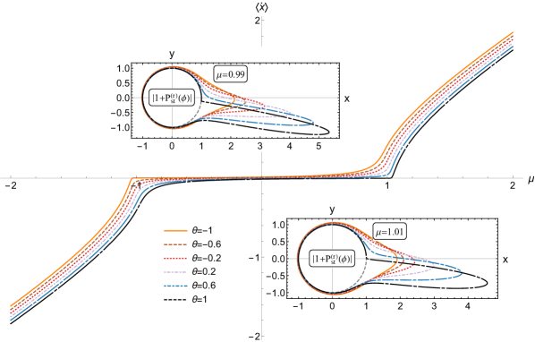
Figure 2: Examples of Eq.(22) (insets) and Eq.(26) (main) for $\rho=-1.5$, $\gamma=1$, $\alpha=0.5$, $\lambda=0.5$, $\Omega=0.1$ and various values of the asymmetry $\theta$. The left-most inset details a case with stable fixed points in the potential ($\mu=0.99$), the right-most inset details a case with no fixed points in the potential ($\mu=1.01$). Both insets are given as a parametric plot governed by Eq.(18).

With $\alpha=0.5$ we expect for the stable noise case ($\lambda=0)$ very heavy tails which will lead to quite diffuse densities. To identify structure we therefore choose for this $\alpha$ relatively large tempering, namely $\lambda=0.5$. The analogue to Fig.1 is shown in Fig.2, where again the average velocity is shown as a function of $\mu$ for different values now of skew $\theta$, and insets show the wrapped densities for two the choices of $\mu$ above and below the threshold $\mu=1$.

The signature feature of Fig.2 is the behaviour around $\mu=1$: we see that for $\theta=1$ (black curve) the average velocity is zero for a small range of values $1<\mu\leq 1.05$; near $\mu=-1$ the same behaviour recurs for $\theta=-1$. Once the skew decreases, $\theta<1$ for $1<\mu\leq 1.05$, and increases $\theta>-1$ for$-1.05\leq\mu<-1$, the average velocity becomes non-zero in these narrow regions. In other words, one-sided tempered stable noise anti-aligned to the tilt may stabilise the particle on average in circumstances where deterministically it should be unstable (namely there is no well). This is stochastic current stabilisation.

These properties are reflected in the wrapped densities in the inset. The left-most inset of Fig.2, for $\mu=0.99$ shows strongly peaked densities just as for the Gaussian case. However, the right-most inset with $\mu=1.01$ also shows a strongly peaked density for $\theta=1$ where the analogous Gaussian case of Fig.1 shows diffusion around the circle (particularly for the corresponding value of $\Omega$). Observe how for both cases of $\mu$, the curve for the one-sided density with $\theta=1$ joins the circle sharply on one side (anti-clockwise from the peak) and more smoothly on the other (clockwise from the peak). This manifests the skew for this case.

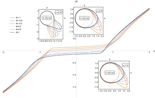
Figure 3: Examples of Eq.(22) (insets) and Eq.(26) (main) for $\rho=-1.5$, $\gamma=1$, $\alpha=1.25$, $\lambda=0.001$, $\Omega=0.1$ and various values of the asymmetry $\theta$. The left-most inset details a case with stable fixed points in the potential ($\mu=0.5$), the middle inset is $\mu=0.99$ and the right-most inset details a case with no fixed points in the potential ($\mu=1.01$). The insets are given as a parametric plot governed by Eq.(18).

We now chose a contrasting case with $\alpha=1.25$, greater than one but still significantly far from Gaussianity, and $\lambda=0.001$ which is close to the stable limit. The corresponding average velocity and wrapped densities are shown in Fig.3, but now for three choices of $\mu$. Now for $-1<\mu<1$ the average velocity no longer vanishes in general except for specific values of $\theta$ at specific values of $\mu$; at such values the skew exactly balances against the tilt. However, unusually, there are regions where the sign of $\langle\dot{x}\rangle$ is opposite to that of $\mu$ for certain ranges of skew $\theta$. For example, for $\theta=1$ (black curve) and $0<\mu<0.7$, $\langle\dot{x}\rangle<0$ the particle is propagating in the negative direction (to the left) even though skew and tilt are positive. For $\theta=-1$ (orange curve) and $-0.7<\mu<0$, $\langle\dot{x}\rangle>0$ so that the particle is propagating in the positive direction (to the right) even though skew and tilt are negative. This is the phenomenon of current reversal.

Examining the wrapped densities, shown in the insets, we see strongly oriented and sharp densities for $\mu=0.5$ across the range of $\theta$, while for $\mu=0.99,1.01$ the densities are mostly diffuse for $\theta>0$, most strongly for $\theta=1$. These assist, to a degree, in understanding the counter-intuitive current reversal. Specifically, we observe that for the one-sided case $\theta=-1$ (orange curve) the heavy tail is in the anti-clockwise direction while the peak is oriented clockwise from the positive horizontal direction. Recalling that all of the cases of $\theta$ correspond to the same mean, we observe that the mode of the distribution shifts further and further clockwise from the axis. This indicates that the heavy tail is in the anti-clockwise direction (in contrast to the $\theta=1$ case). Significantly, for $\alpha>1$ the mode of the distribution lies in the opposite direction from the heavy tail KallRob2017 . The wrapped densities, particularly with the distortions of plotting on a circle, do not convey well the significance of the heavy tail; in KallRob2017 the role of the tail was best represented through Quartile-Quartile plots. Nevertheless, in the case of such small tempering given a heavy tail in the negative direction for $\theta<0$, we obtain a probability mass in the positive direction. So there is a dominance of small jumps in the positive direction. Thus, with small tempering and even subject to positive tilt, there is a net drift in the positive direction. The current reversal arises from this. (We only caution that the threshold for this behaviour cannot immediately be read off the wrapped density plots since they represent the density of $x$ rather than the current density.) A similar phenomenon was observed in the Kuramoto model in KallRob2017 , a point to which we shall return in the final section.

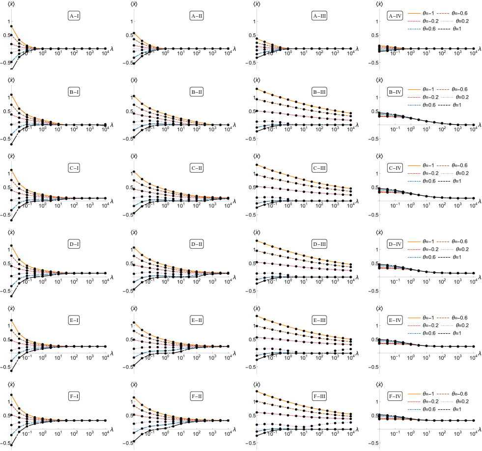
Figure 4: Examples of Eq.(26) for $\rho=-1.5$, $\gamma=1$, $\Omega=0.1$. The tempering $\lambda$ is being varied on the horizontal axis, with various values of the asymmetry $\theta$. Down the rows (A-F) the tilt $\mu$ is varied, with the values $\mu=\{0.1,0.995,1.005,1.01,1.03,1.05\}$ being applied from top to bottom row. Across the columns (I-IV) the fractional power $\alpha$ is varied, with the values $\alpha=\{0.25,0.55,0.85,1.25\}$ applied from left-most to right-most column.

Having examined two selected cases, we now conduct a more general scan across a range of $\lambda$ for representative values of $\alpha$ below and above one and different skew values $\theta$. This is shown in Fig.4. These plots should be compared with Fig.15 in KullCast2012 for tempered stable noise in a (different to ours) ratchet potential without tilt $(\mu=0$). We choose $\mu$ quite far from this regime, and scan in the vicinity of $\mu=1$, namely $0.995\leq\mu\leq 1.05$ and $\alpha=0.25,0.55,0.85,1.25$. But for some comparison we also provide the result for $\mu=0.1$. As $\mu>0$ for all these cases, current reversal corresponds to negative values of $\langle\dot{x}\rangle$ in these plots.

In fact, we observe that current reversal is a generic feature both below the deterministic threshold of $\mu=1$ and above: starting from the top left and scanning across to higher values of $\alpha$, and scanning down with increasing increments in $\mu$. The case shown in KullCast2012 , where they choose $\alpha=1.5$ and two values of $\theta$, shows a current starting negative for small $\lambda$, crossing zero to positive values and then converging to zero; this is hidden in a plot such as panel A-IV in Fig.4. For larger tilt $\mu$ such behaviour moves to $\alpha<1$. For example, panel B-I shows curves for $\theta\approx 0.6$ crossing from negative to positive and then converging to zero. This current reversal occurs not only for the most extreme skew $\theta=1$ but closer to symmetric noise.

We see that for $\mu<1$ and large $\lambda$ the average velocity tends to zero (top two rows); for $\mu>1$ the asymptotic limit is non-zero and positive (third row and below), which corresponds to the deterministic value as tempering suppresses all noise. We also observe that the current reversal ceases above $\alpha=1$ in this region of $\mu$ - recall that in Fig.3 the reversal occurs for $\mu<0.7$.

Within the regimes of current reversal there are always discrete values where $\langle\dot{x}\rangle=0$. However, we also see for $\mu>1$ and $\alpha<1$ regimes where the average velocity vanishes across a continuum of $\lambda$ values before increasing and converging to the deterministic limit - this is most distinct in panel C-II. Thus current stablisation may be sustained across a broad range of $\lambda$ before tempering dampens the noise completely. These demonstrate that current stablisation is linked naturally to current reversal - but the stablisation over a range of $\lambda$ may not be intuitively expected.

Moving to the lower rows we observe that the range of $\lambda$ over which stabilisation occurs shrinks until it becomes only a discrete case of $\lambda$ except for pure one-sided noise with $\theta=1$. For the cases in panels E-III and F-III with $\theta=1$ the average velocity will converge to its non-zero value at $\lambda$ values beyond those plotted here.

V Conclusions and Discussion

We have solved the Fokker-Planck equation for a particle in a one-dimensional tilted ratchet potential under tempered stable Lévy noise and have observed both phenomena of current stabilisation and reversal, particularly in regimes where deterministic or Gaussian considerations would show quite different behaviour.

The essence of the mechanism is the interplay between probability mass around mode of the underlying noise distributions and the heavy tails and how it shifts as $\alpha,\lambda$ are varied. Specifically, for $\alpha>1$ the mode is typically in the opposite direction from the tail for asymmetric noise as discussed in KallRob2017 . This leads to a drift in a direction corresponding to the sign of the mode, which manifests as current reversal for the particle in the tilted ratchet. When $\alpha<1$, due to the induced drift through the form of the noise characteristic function, the mode and heavy tails are in the same direction but with increased mass around the mode and heavier tails. Thus, with tempering, both long range and intermediate range jumps are suppressed so that the effective drift may even drop down to zero with increased skew in the noise. Moreover, tempering moderates current reversal until it assumes the form of current stabilisation. Thus the particular cases of current reversal in KullCast2012 are a special instance of a phenomenon in the presence of tilt in the potential.

As alluded in the introduction, for us the interest in this phenomena arises from our work on the Kuramoto model or related forms. In KallRob2017 and KallRob2017b we have observed a phenomenon of oscillators of zero native frequency nevertheless synchronising to a non-zero net frequency, a drift, that shifts in sign according to the interplay of $\alpha$ and $\lambda$. While general observations of the position of the mode and the heaviness of the tail in those cases provide an heuristic explanation of this phenomena, we argue that the model solved here may provide a deeper insight into this behaviour. Future applications of this idea lie in its exploitation for stochastic control of synchronisation phenomena.

References

References

- (1) P. Reimann, Brownian motors: noisy transport far from equilibrium, Physics reports 361, 57-265, 2002
- (2) B. Linder, M. Kostur and L. Schimansky-Geier, Optimal diffusive transport in a tilted periodic potential, Fluctuation and Noise 1(1), R25-R39, 2001
- (3) D. Hennig, Current control in a tilted washboard potential via time-delayed feedback, Phys.Rev.E 79, 041114, 2009
- (4) C. Mulhern, D. Hennig, Current reversals of coupled driven and damped particles evolving in a tilted potential landscape, Phys.Rev.E 84, 036202, 2011
- (5) K.J. Challis, M.W. Jack, Tight-binding approach to overdamped Brownian motion on a multidimensional tilted periodic potential, Phys.Rev. E 87, 052102, 2013
- (6) A.A. Borovkov, K.A. Borovkov, Asymptotic analysis of random walks: heavy-tailed distributions, Cambridge, UK, 2008
- (7) J.M. Chambers, C.L. Mallows, B.W. Stuck, J. Am. Stat. Assoc, 71 (354), 340-344, 1976
- (8) M.C.K. Tweedie, in Statistics: Applications and New Directions: Proc. Indian Statistical Institute Golden Jubilee International Conference (eds. J. Ghosh, J. Roy) 579-604, 1984
- (9) R.N. Mantegna, H.E. Stanley, Stochastic process with ultraslow convergence to a Gaussian: the truncated Lévy flight, Phys.Rev.Lett. 73, 2946-2949, 1994
- (10) I. Koponen, Analytic approach to the problem of convergence of truncated Lévy flights towards the Gaussian stochastic process, Phys.Rev.E 52, 1197-1199, 1995
- (11) M.M. Meerschaert, F. Sabzikar, Tempered fractional stable motion, J.Theor.Probab. 29, 681-706, 2016
- (12) B. Baeumer, M.M. Meerschaert, Tempered stable Lévy motion and transient super-diffusion, J. Comp.Appl. Math. 233, 2438, 2010
- (13) J. Gajda, M. Magdziarz, Fokker-Planck equation with tempered -stable waiting times: Langevin picture and computer simulation, Phys.Rev.E 82, 011117, 2010
- (14) R. Metzler, J. Klafter, The random walk’s guide to anomalous diffusion: a fractional dynamics approach, Phys.Rep. 339, 1-77, 2000
- (15) G. Jumarie, Fractional Brownian motions via random walk in the complex plane and via fractional derivative. Chaos, Solitons and Fractals 22, 907-925, 2004
- (16) R. Metzler, J. Klafter, The restaurant at the end of the random walk: recent developments in the description of anomalous transport by fractional dynamics, J.Phys.A:Math.Gen. 37, R161-R208, 2004
- (17) S. Jespersen, R. Metzler, H.C. Fogedby, Lévy flights in external force fields: Langevin and fractional Fokker-Planck equations and their solutions, Phys.Rev.E 59, 2736, 1999
- (18) R. Metzler, J. Klafter, From a generalized Chapman-Kolmogorov equation to the fractional Klein-Kramers equation, J.Phys.Chem. B 2000, 3851-3857, 2000
- (19) A. Chechkin, V. Gonchar, J. Klafter, R. Metzler, L. Tanatarov, Stational states of non-linear oscillators driven by L’evy noise, Chemical Physics 284, 233-251, 2002
- (20) M. Magdziarz, A. Weron, Fractional Fokker-Planck dynamics: stochastic representation and computer simulation, Phys.Rev.E 75, 016708, 2007
- (21) A.V. Chechkin, V.Yu. Gonchar, R. Gorenflo, N. Korabel, I.M. Sokolov, Phys.Rev.E 78, 021111, 2008
- (22) K Gorska and K Penson, Lévy stable two-sided distributions: Exact and explicit densities for asymmetric case, Phys. Rev. E 83 (2011) 061125
- (23) A. Kullberg, D. del-Castillo-Negrete, Transport in the spatially tempered, fractional Fokker-Planck equation, J.Phys.A: Math.Theor. 45, 255101, 2012
- (24) D. Reguera, P. Reimann, P. Hänggi, J.M. Rubí, Interplay of frequency-synchronization with noise: current resonance, giant diffusion and diffusion-crests, Europhys.Lett.57 (5), 644-650, 2002
- (25) L. Gammaitoni, P. Hänggi, P. Jung, F. Marchesoni, Rev.Mod.Phys. 70, 223, 1998
- (26) L. Gammaitoni, P. Hänggi, P. Jung, F. Marchesoni, Stochastic resonance: a remarkable idea that changed our perception of noise, Eur.Phys.J.B 69, 1-3, 2009
- (27) Y. Kawamura, Collective phase dynamics of globally coupled oscillators: noise-induced anti-phase synchronization, Physica D 270, 20-29, 2014
- (28) H. Kleinert, Path Integrals in quantum mechanics, statistics, polymer physics and financial markets, World Scientific, New Jersey, London, Singapore, 2009
- (29) D. del-Castillo-Negrete, B.A. Carreras, V.E. Lynch, Nondiffusive transport in plasma turbulence: a fractional diffusion approach, Phys.Rev.Lett. 94, 065003, 2005
- (30) D. del-Castillo-Negrete, V.Yu. Gonchar, A.V. Checkin, Fluctuation-driven directed transport in the presence of Lévy flights, Physica A 387, 6693-6704, 2008
- (31) R.J. Elliott, J. van der Hoek, A general fractional white noise theory and applications to finance, Mathematical Finance 13, 2, 301-330, 2003
- (32) A. Cartea, D. del-Castillo-Negrete, Fractional diffusion models of option prices in markets with jumps, Physica A 374, 749-763, 2007
- (33) J.A. Roberts, T.W. Boonstra, M. Breakspear, The heavy tail of the human brain, Current Opinion in Neurobiology 31, 164-172, 2015
- (34) Y. Kuramoto, Chemical Oscillations, Waves and Turbulence, Springer, Berlin, 1984
- (35) L DeVille, Transitions amongst synchronous solutions in the stochastic Kuramoto model, Nonlinearity 25(5), 2012
- (36) M Freidlin and A Wentzell, Random perturbations and dynamical systems: (2nd Ed.), Springer-Verlag, New-York, 1998
- (37) M.L. Zuparic, A.C. Kalloniatis, Physica D 255, 35-51, 2013
- (38) A Holder, M Zuparic and A Kalloniatis, Gaussian noise and the two-network frustrated Kuramoto model, Physica D 341, 10-32, 2017
- (39) A Kalloniatis and D Roberts, Synchronisation of networked Kuramoto oscillators under stable Lévy noise, Physica A 466 (2017) 476-491
- (40) A Kalloniatis and D Roberts, Synchronisation of networked Kuramoto oscillators under tempered stable Lévy noise, in preparation, 2017
- (41) R. Kawai, H. Masuda, On simulation of tempered stable random variates, J. Comp.Appl. Math. 235, 2873, 2011
- (42) A. Cartea and D. del-Castillo-Negrete, Fluid limit of the continuous-time random walk with general Lévy jump distribution functions, Phys. Rev. E (2007) 041105
- (43) D del-Castillo-Negrete, Anomalous transport in the presence of truncated Lévy flights. In: J Klafter, S Lim and R Metzler (Ed.) Fractional dynamics: Recent advances. World Scientific, Singapore (2012) p.129-157.
- (44) I Podlubny, Fractional differential equations, Academic Press, San Diego, (1999)
- (45) S Samko, A Kilbas and O Marichev, Fractional integrals and derivatives: Theory and applications, CRC Press, London, (1993)
- (46) K. Sato, Lévy processes and infinite divisibility, Cambridge University Press, 1999
- (47) N Berglund, B Fernandez and B Gentz, Metastability in interacting nonlinear stochastic differential equations: I. From weak coupling to synchronization, Nonlinearity 20, 2007
- (48) R Stratonovich, Topics in the theory of random noise: Vol III, Gordon and Breach, New-York, 1967
- (49) N.I. Fisher, Statistical analysis of circular data, Cambridge University Press, 1996
- (50) H Risken, The Fokker-Planck Equation, (2nd Ed.), Springer, Heidelberg, (1989)