Analytic solution to space-fractional Fokker-Planck equations for tempered-stable Lévy distributions with spatially linear, time-dependent drift

Abstract

We derive analytic solutions for the full time dependence of space-fractional Fokker-Planck equations corresponding to stochastic Langevin equations with additive tempered-stable Lévy noise terms. The drift terms are generalised to be spatially linear, but may contain arbitrary time dependence such that no steady-state solution is available, even for the deterministic system.

Keywords: Fokker-Planck, tempered-stable Lévy noise, hypergeometric function

1 Introduction

The steady-state behaviour of many stochastic dynamical systems, while genuinely informative, is often the limit of what is studied by many researchers, particularly for non-Gaussian noise models. Analytic approaches are lacking when there is no steady-state behaviour, even deterministically. Here we solve the time-dependence of Fokker-Planck (FP) probability densities in the presence of tempered stable noise.

The classical method of solving both steady-state and time-dependent probability density functions for Fokker-Planck equations with additive Gaussian noise, the Ornstein-Uhlenbeck process, is covered in works such as Risken [1]. Time-dependence of some non-Gaussian FP equations, often based on multiplicative noise Langevin equations (for example a noisy form of the logistic equation [2] drawing upon applications in financial mathematics by Linetsky [3]), may be obtained by a variable transformation in a Gaussian system. Here various orthogonal polynomials capture the space-dependence of the system; exponential decay weighted by an eigenvalue of the Sturm-Liouville operator gives the time-dependence. This generalises the role of Hermite polynomials for the Ornstein-Uhlenbeck case corresponding to additive Gaussian noise in the associated Langevin system. Thus, various classical continuous orthogonal polynomials appear, leading to a mixed discrete-continuous spectrum for the time dependence [4].

Moving beyond Gaussian based noise models is a growing area of interest. This is because many complex systems exhibit ‘fat-tail’ phenomena [5] which can lead to large spatial jumps, or large waiting times, such as in financial markets [6, 7], transport in plasmas [8, 9] and brain activity [10]. The Lévy stable distribution is a valuable model for the underlying stochastic system, where a power-law tail is modelled by an exponent $\alpha$. For $\alpha<2$ one obtains what is commonly known as fractional or anomalous diffusion [11, 12]. Here we find generalisations of the Ornstein-Uhlenbeck result where the Hermite polynomials in the spatial part of the probability density function are replaced by Fox’s H functions [13]. Further generalisations of the external force, though limited to steady-state solutions can be found in Chechkin et al. [14]. We focus in this paper on spatial jumps; on large waiting times see [15, 17, 16, 18] or the bi-fractional case [19, 20, 21].

A key property of stable Lévy noise is that because of the heavy tails there are no finite moments beyond the first for $1<\alpha<2$, and not even the first for $0<\alpha<1$, a problem when fitting finite empirical datasets. Truncating with a hard cut-off [22, 23] or, less severely, tempering the noise [24, 25] are two alternatives. The latter case is of interest to us here. A characteristic scale $\lambda$ moderates the extreme asymptotics of the tails rendering all moments finite. Thus far, only numerical [26, 27, 28] (the latter for time-fractional) or steady-state [29] solutions of Fokker-Planck equations have been obtained for this case — though the equations are solved up to a numerically computed inverse Fourier transform. We extend this approach to cover full time-dependence. However, as a by-product we can generalise to the time-dependent solution the case of stable noise, where the Fourier-transform may be explicitly computed. We focus on the spatially-tempered fractional Fokker-Planck equation but seek the solve as explicitly as possible for the entire time-dependence, both for cases where steady-state behaviour is approached but also where the time-dependence may be an ongoing regular dynamic, such as periodicity.

Our main motivation for obtaining analytic solutions to such generalised Ornstein-Uhlenbeck processes lies in their ability to provide insights and understanding into networked complex systems. Dynamical processes on networks remains an ongoing research area with far reaching physical, biological, social/organisational and chemical applications [30]. The paradigmatic Kuramoto model of phase oscillators [31] offers an accessible mathematical formulation of networked dynamics which displays surprising emergent behaviour; for reviews refer to [32, 33, 34]. Our particular interest lies in understanding the model under stochastic influence. The deterministic system can be reduced to a system of decoupled first-order linear differential equations after linearisation close to synchronisation, where the system decays monotonically to pure frequency synchronisation [35]. With additive Gaussian noise the system becomes an Ornstein-Uhlenbeck system [36], and with additive tempered Lévy noise this is the tempered fractional Ornstein-Uhlenbeck system [37]; the drift in these cases is purely space-dependent. Recently, the authors explored the cooperative and competitive behaviour displayed by the frustrated 2-network Kuramoto-Sakaguchi model [38], both deterministically [39] and under the influence of additive Gaussian noise [40]. The relevant approximation for this system involves searching states below the threshold for frequency synchronisation, where 2 or more internally synchronised populations may be in relative time-dependent oscillatory motion. In this case the drift terms of the corresponding Langevin equations (although spatially linear) are generally time-dependent. The latter work used a key result from Polyanin [41] which we show may be generalised to tempered stable noise, thus explaining at least one physics application of the results pursued in this work.

In the next section we set-up our formalism for the tempered-fractional Fokker-Planck equations, particularly using the Fourier transform approach. In section 3 we then step through the solution, detailing both the stable case, and the more general tempered-stable case. In section 4 we give some numerical examples which illustrate utility of this work by choosing drift terms which do not accommodate steady state density solutions. We also validate our analytic expression through numerical comparison with an alternate solution which is more computationally intensive (but more straightforwardly obtained). Finally in section 5 we offer conclusions and future applications of this work.

2 Tempered-fractional-Fokker-Planck equations

2.1 Fractional Langevin equations

We consider the fractional version of a Langevin equation

$$\dot{x}=q(x,t)+L^{\alpha,\theta,\lambda}(t),$$ (1)

where $L^{\alpha,\theta,\lambda}(t)$ is a tempered stable Lévy process in time described by parameters $\alpha,\theta,\lambda$. Here $\alpha\in(0,1)\cup(1,2]$ is the fractional power, governing the heavy-law tail of the distribution for $L$, $\theta\in[-1,1]$ is an asymmetry generating skew in the distribution, and $\lambda\in(0,\infty)$ is a tempering parameter that exponentially suppresses large jumps in the process $L$. For $\alpha=2$, the Lévy noise term in Eq. (1) becomes Gaussian. The case $\alpha=1$ is known as the Cauchy process; we do not consider it in this work due to the ‘pathological’ property of none of its moments formally existing [42].

2.2 Reimann-Liouville fractional derivatives

The probability density $P(x,t)$ associated with the tempered-stable Lévy process given by Eq. (1) satisfies the Fokker-Planck equation [43]

$$\frac{\partial}{\partial t}P(x,t)=\left(\Omega\partial^{\alpha,\theta,\lambda}_{x}-\frac{\partial}{\partial x}q(x,t)\right)P(x,t),\;\;P(x,0)=\delta(x-y),$$ (2)

where $\Omega\in(0,\infty)$ is the diffusion constant, which becomes the variance of the process in the Gaussian limit. Additionally, the operator $\partial^{\alpha,\theta,\lambda}_{x}$ is the tempered-fractional-diffusion operator, given explicitly as [29]

$$\partial^{\alpha,\theta,\lambda}_{x}={\cal D}^{\alpha,\theta,\lambda}_{x}+v^{\alpha,\theta,\lambda}\frac{\partial}{\partial x}+\nu^{\alpha,\lambda},$$ (3)

where $v^{\alpha,\theta,\lambda}$ and $\nu^{\alpha,\lambda}$ are additional drift and source/sink terms given by

$$v^{\alpha,\theta,\lambda}=\left\{\begin{array}[]{cl}0,&\alpha\in(0,1)\\ \frac{\alpha\theta\lambda^{\alpha-1}}{|\cos\frac{\pi\alpha}{2}|}&\alpha\in(1,2)\end{array}\right.,\;\;\nu^{\alpha,\lambda}=\frac{\lambda^{\alpha}}{\cos\frac{\pi\alpha}{2}}.$$ (4)

The operator ${\cal D}^{\alpha,\theta,\lambda}_{x}$ is called the $\lambda$-truncated fractional derivative of order $\alpha$, given by

$${\cal D}^{\alpha,\theta,\lambda}_{x}=l(\theta)e^{-\lambda x}\,_{-\infty}D^{\alpha}_{x}e^{\lambda x}-r(\theta)e^{\lambda x}\,_{x}D^{\alpha}_{\infty}e^{-\lambda x},$$ (5)

where the operators $\,{}_{-\infty}D^{\alpha}_{x}$ and $\,{}_{x}D^{\alpha}_{\infty}$ are the Riemann-Liouville derivatives defined as [44]

$$\begin{split}e^{-\lambda x}\,_{-\infty}D^{\alpha}_{x}e^{\lambda x}f(x)=\frac{e^{-\lambda x}}{\Gamma(m-\alpha)}\frac{\partial^{m}}{\partial x^{m}}\int^{x}_{-\infty}\frac{d\zeta e^{\lambda\zeta}}{(x-\zeta)^{\alpha+1-m}}f(\zeta)\\ e^{\lambda x}\,_{x}D^{\alpha}_{\infty}e^{-\lambda x}f(x)=\frac{(-1)^{m}e^{\lambda x}}{\Gamma(m-\alpha)}\frac{\partial^{m}}{\partial x^{m}}\int^{\infty}_{x}\frac{d\zeta e^{-\lambda\zeta}}{(\zeta-x)^{\alpha+1-m}}f(\zeta),\end{split}$$ (6)

for $\alpha-1<m<\alpha$. These can be equivalently defined in Fourier space [45, 46]

$$\begin{split}{\cal F}\left[e^{-\lambda x}\,_{-\infty}D^{\alpha}_{x}e^{\lambda x}f(x)\right]=(\lambda-ik)^{\alpha}\hat{f}(k)\\ {\cal F}\left[e^{\lambda x}\,_{x}D^{\alpha}_{\infty}e^{-\lambda x}f(x)\right]=(\lambda+ik)^{\alpha}\hat{f}(k),\end{split}$$ (7)

where

$$\begin{split}{\cal F}\left[f(x)\right]=\int^{\infty}_{-\infty}dxe^{ikx}f(x)=\hat{f}(k)\\ {\cal F}^{-1}\left[\hat{f}(k)\right]=\int^{\infty}_{-\infty}\frac{dk}{2\pi}e^{-ikx}\hat{f}(k)=f(x).\end{split}$$ (8)

The weighting factors

$$l(\theta)=\frac{\theta-1}{2\cos\frac{\pi\alpha}{2}},\;\;r(\theta)=\frac{\theta+1}{2\cos\frac{\pi\alpha}{2}},$$ (9)

determine the asymmetry imposed on each of the Riemann-Liouville derivatives. The introduction of the exponential decay terms to the Reimann-Liouville derivatives in Eqs. (5) and (6) has the effect of tempering the stable process. That is, for all $\alpha\in(0,1)\cup(1,2)$, all moments of the corresponding tempered-stable process ($\lambda>0)$ are finite, marking a clear distinction from stable ($\lambda=0$) processes where only the first moment of the $\alpha\in(1,2)$ is finite.

2.3 Spatially linear time-dependent drift terms

We generalise the drift term $q(x,t)$ in Eqs. (1) and (2) from the Ornstein-Uhlenbeck form to include time-dependent coefficients

$$q(x,t)=\beta(t)-\gamma(t)x,\;\;\gamma(t)>0,$$ (10)

where $\beta(t)$ and $\gamma(t)$ are general time-dependent functions. Hence, the explicit form of the tempered-fractional-Fokker-Planck equation (TFFP) becomes

$$\frac{\partial}{\partial t}P(x,t)=\left[\Omega{\cal D}^{\alpha,\theta,\lambda}_{x}+\left(\gamma(t)x+\Omega v^{\alpha,\theta,\lambda}-\beta(t)\right)\frac{\partial}{\partial x}+\left(\gamma(t)+\Omega\nu^{\alpha,\lambda}\right)\right]P(x,t).$$ (11)

For the Gaussian limit, i.e. $\partial^{\alpha,\theta,\lambda}_{x}=\frac{\partial^{2}}{\partial x^{2}}$, Polyanin [41] gives the necessary nonlinear transformations which result in the Gaussian equivalent of Eq. (11) becoming the standard heat equation. Indeed, this technique enabled the analytical investigation of clustering effects in the frustrated Kuramoto model under the influence of Gaussian white noise [40]. In this work we follow a similar strategy and apply a variant of the nonlinear transformations given in [41] to Eq. (11) to obtain a tempered-fractional form of the heat equation with complications in the tempering. We then apply the Fourier transform to this ‘heat equation’, solving it explicitly in Fourier space with the appropriate initial condition. The final solution is obtained by performing the inverse Fourier transform.

3 Analytical solution to the tempered-fractional-Fokker-Planck equation

3.1 Nonlinear transformations

Generalising Polyanin [41, section 1.8.3.6] we consider the following set of transformations to ${P}(x,t)$, $x$ and $t$:

$$\begin{split}{P}(x,t)={Q}(z,\tau)e^{\int^{t}_{0}d\xi\left(\gamma(\xi)+\Omega\nu^{\alpha,\lambda}\right)},\;\;\tau=\int^{t}_{t^{\prime}}d\xi e^{\alpha\int^{\xi}_{0}d\vartheta\gamma(\vartheta)}\\ z=xe^{\int^{t}_{0}d\xi\gamma(\xi)}+\phi(t),\;\;\phi(t)=\int^{t}_{0}d\xi e^{\int^{\xi}_{0}d\vartheta\gamma(\vartheta)}\left(\Omega v^{\alpha,\theta,\lambda}-\beta(\xi)\right),\end{split}$$ (12)

for $t^{\prime}\in\mathbb{R}$. Doing so results in the differential operator relations

$$\begin{split}\frac{\partial}{\partial t}=e^{\alpha\int^{t}_{0}d\xi\gamma(\xi)}\frac{\partial}{\partial\tau}+e^{\int^{t}_{0}d\xi\gamma(\xi)}\left(\gamma(t)x+\Omega v^{\alpha,\theta,\lambda}-\beta(t)\right)\frac{\partial}{\partial z}\\ \frac{\partial}{\partial x}=e^{\int^{t}_{0}d\xi\gamma(\xi)}\frac{\partial}{\partial z}.\end{split}$$ (13)

Applying Eqs. (12) and (13) to Eq. (11) we obtain

$$e^{\alpha\int^{t}_{0}d\xi\gamma(\xi)}\frac{\partial}{\partial\tau}{Q}(z,\tau)=\Omega{\cal D}^{\alpha,\theta,\lambda}_{x}{Q}(z,\tau),$$ (14)

with the initial condition ${Q}(z,\tau(t=0))=\delta(z-y)$. We note that the $\lambda$-truncated fractional derivative of order $\alpha$ still contains the argument $x$, as opposed to $z$. This is removed by change of variables in the Riemann-Liouville derivatives of Eq. (6):

$$e^{-\lambda x}\,_{-\infty}D^{\alpha}_{x}e^{\lambda x}{Q}(z,\tau)=\frac{e^{-\lambda x}}{\Gamma(m-\alpha)}\frac{\partial^{m}}{\partial x^{m}}\int^{x}_{-\infty}\frac{d\zeta e^{\lambda\zeta}{Q}\left(\zeta e^{\int^{t}_{0}d\xi\gamma(\xi)}+\phi(t),\tau\right)}{(x-\zeta)^{\alpha+1-m}}$$

$$=e^{\alpha\int^{t}_{0}d\xi\gamma(\xi)}\frac{e^{-\frac{\lambda}{e^{\int^{t}_{0}d\xi\gamma(\xi)}}z}}{\Gamma(m-\alpha)}\frac{\partial^{m}}{\partial z^{m}}\int^{z}_{-\infty}\frac{d\mu e^{\frac{\lambda}{e^{\int^{t}_{0}d\xi\gamma(\xi)}}\mu}{Q}\left(\mu,\tau\right)}{(z-\mu)^{\alpha+1-m}}$$ (15)

$$=e^{\alpha\int^{t}_{0}d\xi\gamma(\xi)}e^{-\frac{\lambda}{e^{\int^{t}_{0}d\xi\gamma(\xi)}}z}\,_{-\infty}D^{\alpha}_{z}e^{\frac{\lambda}{e^{\int^{t}_{0}d\xi\gamma(\xi)}}z}{Q}(z,\tau),$$

where we have made the substitutions $xe^{\int^{t}_{0}d\xi\gamma(\xi)}=z-\phi(t)$ and $\zeta e^{\int^{t}_{0}d\xi\gamma(\xi)}=\mu-\phi(t)$ in the second line of the above expression. One can immediately show that an equivalent relation holds for the remaining Riemann-Liouville derivative, leading to

$${\cal D}^{\alpha,\theta,\lambda}_{x}{Q}(z,\tau)=e^{\alpha\int^{t}_{0}d\xi\gamma(\xi)}{\cal D}^{\alpha,\theta,\frac{\lambda}{(d\tau/dt)^{1/\alpha}}}_{z}{Q}(z,\tau).$$ (16)

Hence, Eq. (14) becomes

$$\frac{\partial}{\partial\tau}{Q}(z,\tau)=\Omega{\cal D}^{\alpha,\theta,\frac{\lambda}{(d\tau/dt)^{1/\alpha}}}_{z}{Q}(z,\tau).$$ (17)

Applying the Fourier transform Eq. (8) to Eq. (17), one obtains an ordinary differential equation with respect to $\tau$ which has the solution

$$\hat{{Q}}(k,\tau)=\kappa(k)\exp\left\{\Omega\left[l(\theta)\int d\tau\left(\frac{\lambda}{\left(\frac{d\tau}{dt}\right)^{1/\alpha}}-ik\right)^{\alpha}-r(\theta)\int d\tau\left(\frac{\lambda}{\left(\frac{d\tau}{dt}\right)^{1/\alpha}}+ik\right)^{\alpha}\right]\right\},$$ (18)

where $\kappa(k)$ is the constant of integration to be determined by the initial condition:

$$\hat{Q}\left(k,\tau(t=0)\right)=e^{iky}.$$ (19)

We now solve Eq. (18) for the following two scenarios:

• $\lambda=0$ and general $\gamma(t)$, where we rely on the main results from [47] to obtain an explicit expression for the inverse Fourier transform with time dependence;

• $\lambda\neq 0$ and $\gamma(t)=\gamma\in\mathbb{R}$, where there is no known analytic expression for the inverse Fourier transform, so that we must rely on numerical integration in the final step.

3.2 Stable solution

We consider first $\lambda=0$. Here we set $t^{\prime}=0$ in Eq. (12) so that $\tau(t=0)=0$. In this case, Eq. (18) becomes [37]

$$\hat{{Q}}(k,\tau)=e^{iky}\exp\left[-\Omega\tau|k|^{\alpha}\left(1+i\theta\textrm{sgn}(k)\tan\frac{\pi\alpha}{2}\right)\right].$$ (20)

Applying the inverse Fourier transform operation we obtain the Lévy-Khinchine formula,

$${Q}(z,\tau)=\frac{1}{\pi\omega}\mathrm{Re}\int^{\infty}_{0}dpe^{-ip\frac{(z-y)}{\omega}}\exp\left(-p^{\alpha}e^{i\frac{\pi\chi}{2}}\right),$$ (21)

where we have used the change of variables

$$\theta=\frac{\tan\frac{\pi\chi}{2}}{\tan\frac{\pi\alpha}{2}},\;\;p=\omega k,\;\;\omega=\left(\frac{\Omega\tau}{\cos\frac{\pi\alpha}{2}}\right)^{1/\alpha}.$$ (22)

If $\alpha$ and $\chi$ are rational numbers the inverse Fourier transform may be explicitly evaluated. Specifically, for the integers $\{l,k,r\}$ we require,

$$\alpha=\frac{l}{k},\;\;\chi=\frac{l-2r}{k}\textrm{ where }\left\{\begin{array}[]{ccc}0<\frac{l}{k}<1,&0\leq r\leq l,&\textrm{ for $\alpha\in(0,1)$}\\ 1<\frac{l}{k}\leq 2,&l-k\leq r\leq k,&\textrm{ for $\alpha\in(1,2]$}\end{array}\right.,$$ (23)

to obtain the following analytic expression for ${Q}(z,\tau)$

$${Q}(z,\tau)=\frac{1}{\omega}\sum^{M-1}_{j=1}\frac{c_{j}(l,k,r)}{(\frac{z-y}{\omega})^{1\mp\frac{jl}{M}}}\,_{m+1}F_{M}\left(\left.\begin{array}[]{c}1,\;\Delta\left(m,\frac{1+jm}{M}\right)\\ \Delta\left(M,j+1\right)\end{array}\right|\frac{m^{m}(\frac{z-y}{\omega})^{\pm l}}{(-1)^{r-M}M^{M}}\right),$$ (24)

where $M=\max(l,k)$, $m=\min(l,k)$, the upper and lower signs are used for the cases $\alpha\in(0,1)$ and $\alpha\in(1,2]$ respectively. Here, $\,{}_{m+1}F_{M}$ is the generalised hypergeometric function, $\Delta(i_{1},i_{2})$ is convenient notation for the parameter list,

$$\Delta(i_{1},i_{2})=\left\{\frac{i_{2}}{i_{1}},\frac{i_{2}+1}{i_{1}},\dots,\frac{i_{1}+i_{2}-1}{i_{1}}\right\},$$ (25)

and the coefficients $c_{j}(l,k,r)$ are given by,

$$c_{j}(l,k,r)=\frac{M^{\frac{1}{2}-j}m^{\frac{1}{2}+\frac{jm}{M}}}{2^{-r}(2\pi)^{\frac{l+k}{2}}}\frac{\left[\prod^{j}_{i=1}\Gamma\left(\frac{i-j-1}{M}\right)\right]\left[\prod^{M}_{i=j+2}\Gamma\left(\frac{i-j-1}{M}\right)\right]}{\left[\prod^{m-1}_{i=0}\Gamma\left(\frac{j}{M}+\frac{i+1}{m}\right)\right]^{-1}\left[\prod^{r-1}_{i=0}\sin\left(\pi\left\{\frac{i}{r}+\frac{j}{M}\right\}\right)\right]^{-1}}.$$ (26)

Eq. (24) is given as the main result of Gorska and Penson [47] which involves the application of the Mellin transform and subsequent Meijer-G function identities to Eq. (21).

Thus, with Eqs. (12) and (24) with rational fractions for $\alpha$ and $\chi$, the density ${P}(x,t)$ for the $\lambda=0$ case is

$${P}(x,t)={Q}\left(xe^{\int^{t}_{0}d\xi\gamma(\xi)}+\phi(t),\int^{t}_{0}d\xi e^{\alpha\int^{\xi}_{0}d\vartheta\gamma(\vartheta)}\right)e^{\int^{t}_{0}d\xi\gamma(\xi)}.$$ (27)

For irrational $\alpha$ and $\chi$ in the stable $\lambda=0$ case, numerical integration is still required for the inverse Fourier transform.

3.3 Tempered-stable solution

Turning to $\lambda\neq 0$, we set $t^{\prime}=-\infty$ in Eq. (12) so that $\tau(t=0)=1/(\alpha\gamma)$. In order to proceed we set $\gamma(t)=\gamma\in\mathbb{R}_{+}$, which leads to

$$\left(\frac{\lambda}{\left(\frac{d\tau}{dt}\right)^{1/\alpha}}\mp ik\right)^{\alpha}=\left(\frac{\varphi}{\tau^{1/\alpha}}\mp ik\right)^{\alpha}\;\;\textrm{where}\;\;\varphi=\frac{\lambda}{(\alpha\gamma)^{1/\alpha}}.$$ (28)

The integrals can then be evaluated using the hypergeometric expressions

$$\begin{split}\int d\tau\left(\frac{\varphi}{\tau^{1/\alpha}}\mp ik\right)^{\alpha}=(\mp ik)^{\alpha}\tau\,_{2}F_{1}\left(\left.\begin{array}[]{cc}-\alpha,&-\alpha\\ &1-\alpha\end{array}\right|\mp\frac{i\varphi}{\tau^{1/\alpha}k}\right)\\ =\left(\varphi\mp i\tau^{1/\alpha}k\right)^{\alpha}\,_{2}F_{1}\left(\left.\begin{array}[]{cc}-\alpha,&1\\ &1-\alpha\end{array}\right|\frac{\varphi}{\varphi\mp i\tau^{1/\alpha}k}\right)\\ ={Y}_{\mp}(k,\tau),\end{split}$$ (29)

where we have used Abramowitz and Stegun [48, Eq. (15.3.4)] to generate the second line of Eq. (29). Hence the Fourier transform of the TFFP density is

$$\hat{{Q}}(k,\tau)=\kappa(k)\exp\left\{\Omega\left[l(\theta){Y}_{-}(k,\tau)-r(\theta){Y}_{+}(k,\tau)\right]\right\},$$ (30)

where the integration constant $\kappa(k)$ is given by

$$\kappa(k)=e^{iky}\exp\left\{-\Omega\left[l(\theta){Y}_{-}\left(k,\frac{1}{\alpha\gamma}\right)-r(\theta){Y}_{+}\left(k,\frac{1}{\alpha\gamma}\right)\right]\right\}.$$ (31)

Additionally, applying the convenient notation

$${Z}(k,\tau)={Y}_{-}\left(k,\tau\right)-{Y}_{-}\left(k,\frac{1}{\alpha\gamma}\right),$$ (32)

we obtain

$$\hat{{Q}}(k,\tau)=e^{iky}\exp\left\{-\frac{\Omega}{\cos\frac{\pi\alpha}{2}}\left[\mathrm{Re}({Z}(k,\tau))-i\theta\mathrm{Im}({Z}(k,\tau))\right]\right\}.$$ (33)

Hence with Eqs. (12) and (33) the solution for the density ${\cal P}(x,t)$ becomes

$${P}(x,t)=e^{\left(\gamma+\Omega\nu^{\alpha,\lambda}\right)t}\mathrm{Re}\int^{\infty}_{0}\frac{dk}{\pi}e^{-ik(xe^{\gamma t}+\phi(t))}\hat{Q}\left(k,\frac{1}{\alpha\gamma}e^{\alpha\gamma t}\right),$$ (34)

where we have reduced the problem of computing the probability density to a one-dimensional integral.

4 Numerical examples and validation

4.1 Damped oscillatory drift

To illustrate the time-dependence of the solution we choose the drift to have the form

$$\beta(t)=1-e^{-t}+\frac{1}{4}\sin\pi t.$$ (35)

This incorporates elements of exponential decay, but not to a constant. Contrastingly we choose a constant for the coefficient of $x$ in $q(x,t)$, specifically $\gamma=3$. We fix the noise strength $\Omega=1$ and asymmetry $\theta=0.9$. We plot ${P}(x,t)$ for a range of $\alpha$ above and below $\alpha=1$, and increasing $\lambda$, through applying the NIntegrate function in Mathematica^® 10.4, using the AdaptiveQuasiMonteCarlo method. In figure 1 we show plots for $\alpha=0.55$ (top row) and $1.15$ (bottom row) with $\lambda=0.001,0.05$ and $0.9$ (left to right). Additionally we remark that each of the six panels’ first time step is $t=0.1$.

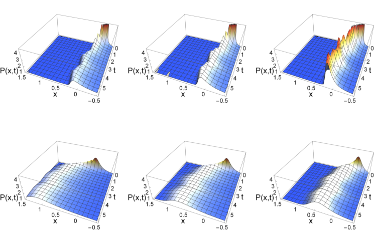
Figure 1: Plots of the time-dependent probability density function ${P}(x,t)$ using Eq. (34) with $\beta(t)=1-e^{-t}+\frac{1}{4}\sin\pi t$, $\theta=0.9$, $y=-0.3$, $\Omega=1$, $\gamma=3$. Top row: $\alpha=0.55$, left $\lambda=0.001$, middle $\lambda=0.05$, right $\lambda=0.9$. Bottom row: $\alpha=1.15$, left $\lambda=0.001$, middle $\lambda=0.05$, right $\lambda=0.9$.

We observe for increasing $\lambda$ the peaking of the density and, concurrently, exposing the time-dependence. Specifically, we see the decay from the initial condition down to the oscillatory behaviour. For both values of $\alpha$ we observe the asymmetry and the heavy-tail in the negative direction. The key difference between $\alpha<1$ and $\alpha>1$ is also evident: the plots in the top row show the cusp like behaviour characteristic of the former case whereas the lower row is smoother, more closely approaching Gaussian shapes. The most significant difference between the two cases is the induced drift in the $\alpha<1$ case. We note that at large $t$, $\beta(t)$ oscillates about unity. In the probability density for $\alpha<1$ this oscillation is shifted in the negative direction. For $\alpha>1$, the density oscillates closer to what may be expected deterministically.

4.2 Numerical validation

In order to validate Eq. (34), and the plots provided in figure 1, we compare outputs from Eq. (34) to a more direct and well known method of solution to Eq. (2): the method of characteristics [49]. Through comparing outputs to a more elementary method of solution (though with the downside of being more computationally intensive) we are able to ensure that Eq. (34) is indeed correct.

To begin we perform a Fourier transform on Eq. (2) to obatin the first order partial differential equation

$$\begin{split}\left(\frac{\partial}{\partial t}+\gamma k\frac{\partial}{\partial k}\right)\hat{{P}}(k,t)=\left(\Omega\Lambda(k)+ik\beta(t)\right)\hat{{P}}(k,t),\;\;\hat{{P}}(k,0)=e^{iky},\\ \textrm{where }\;\;\Lambda(k)=l(\theta)(\lambda-ik)^{\alpha}-r(\theta)(\lambda+ik)^{\alpha}-ikv^{\alpha,\theta,\lambda}+\nu^{\alpha,\lambda}.\end{split}$$ (36)

Following Evans [49, Chapter 3], Eq. (36) can be recast as following characteristic ordinary differential Initial Value Problems (IVPs)

$$\begin{split}\frac{d}{d\xi}t(\mu,\xi)=1,&\;\;t(\mu,0)=0,\\ \frac{d}{d\xi}k(\mu,\xi)=\gamma k,&\;\;k(\mu,0)=\mu,\\ \frac{d}{d\xi}\hat{{P}}(\mu,\xi)=\left(\Omega\Lambda(k)+ik\beta(t)\right)\hat{{P}},&\;\;\hat{{P}}(\mu,0)=e^{i\mu y},\end{split}$$ (37)

for parametric variables $\mu$ and $\xi$.

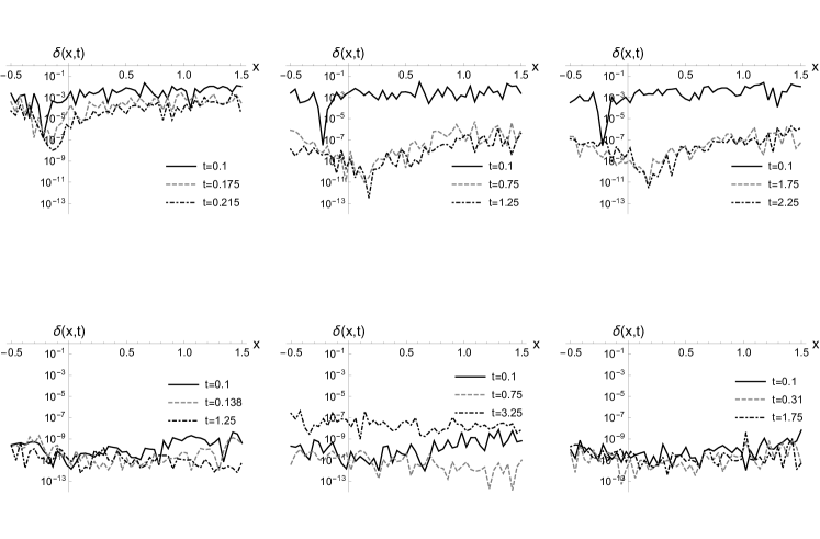
Figure 2: Plots for $\delta(x,t)$: logarithmic plots of the modulus of difference between the probability density function calculated through Eq. (40), and Eq. (34). Parameter choices for each plot are equivalent to figure 1: $\beta(t)=1-e^{-t}+\frac{1}{4}\sin\pi t$, $\theta=0.9$, $y=-0.3$, $\Omega=1$, $\gamma=3$ common for all. Top row: $\alpha=0.55$, left $\lambda=0.001$, middle $\lambda=0.05$, right $\lambda=0.9$. Bottom row: $\alpha=1.15$, left $\lambda=0.001$, middle $\lambda=0.05$, right $\lambda=0.9$.

Solving the first two IVPs in Eq. (37) reveals

$$\begin{array}[]{l}t(\mu,\xi)=\xi\\ k(\mu,\xi)=\mu e^{\gamma\xi}\end{array}\Rightarrow\begin{array}[]{ll}\xi(k,t)=t\\ \mu(k,t)=ke^{-\gamma t}\end{array}.$$ (38)

Hence, the solution to the third IVP in Eq. (37) is

$$\begin{split}&\hat{{P}}(\mu,\xi)=e^{i\mu y}\exp\left[\int^{\xi}_{0}dq\left(\Omega\Lambda\left(\mu e^{\gamma q}\right)+i\mu e^{\gamma q}\beta(q)\right)\right]\\ \Rightarrow\;\;&\hat{{P}}(k,t)=e^{ike^{-\gamma t}y}\exp\left[\int^{t}_{0}dq\left(\Omega\Lambda\left(ke^{\gamma(q-t)}\right)+ike^{\gamma(q-t)}\beta(q)\right)\right].\end{split}$$ (39)

To the best of our knowledge there is no analytic form to the integral in Eq. (39), equivalent to the result of Eq. (33) as a solution to Eq. (18). Thus, in order to calculate the probability density, we are required to perform 2 integrals in the form,

$${P}(x,t)=\frac{1}{2\pi}\int^{\infty}_{-\infty}dke^{-ikx}\hat{{P}}(k,t),$$ (40)

for $\hat{{P}}(k,t)$ given by Eq. (39).

In figure 2 (generated using the same software and method as figure 1) we give the logarithmic plot of the modulus of the difference between the numerical calculations of Eq. (40), and Eq. (34) (labeled as $\delta(x,t)$) for various time instances. Each of the six panels corresponds to the same parameter choices given in figure 1, given explicitly in the caption. Visual inspection of figure 2 shows that the difference between calculating $P(x,t)$ numerically through either Eq. (34) or Eq. (40) is quite small, rarely exceeding $10^{-2}$. Macroscopically, we notice that the values for $\delta(x,t)$ on the bottom panels are generally much lower than those for the top panels, especially for small $t$. A likely explanation for this observation is the more ‘delta-function-like’ behaviour of the densities for $\alpha=0.55$ at $t=0.1$. Indeed, we notice that the remaining curves on the top left panel, for $t=\{0.175,0.215\}$, display greater values of $\delta(x,t)$ than the curves for $t=\{0.75,1.25\}$ and $t=\{1.75,2.25\}$ for the top-middle and top-right panels respectively. Referring back to the top panels in figure 1, we see that the densities are quite highly peaked for small times, only losing this behaviour at approximately $t>0.7$, thus explaining why the corresponding $\delta(x,t)$ plots in the top-middle and top-right panels are much lower. Almost counter-intuitively however, the sharp ‘dips’ in the top panels for the $t=0.1$ plots correspond to the peaks of the densities for this particular time, all of which rise higher than a value of $30$. The corresponding plots of $P(x,0.1)$ for $\alpha=0.55$ and various choices of $\lambda$ are given in figure 3.

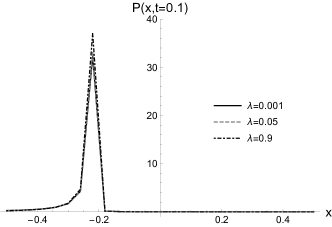
Figure 3: Plots for $P(x,0.1)$ generated from Eq. (34). Parameter choices for each plot are $\beta(t)=1-e^{-t}+\frac{1}{4}\sin\pi t$, $\theta=0.9$, $y=-0.3$, $\Omega=1$, $\gamma=3$ and $\alpha=0.55$.

The plots given in the bottom panels of figure 2 contain no surprises. The corresponding density plots in figure 1 for $\alpha=1.15$ clearly show much more diffuse behaviour for $t\geq 0.1$ than those for $\alpha=0.55$. Correspondingly, the values of $\delta(x,t)$ are much smaller for these parameter choices, rarely rising above $10^{-7}$, and achieving values as low as $10^{-13}$. Thus, through the comparison of Eq. (34) with Eq. (40) over a range of parameter values, we conclude that the analytical result offered by Eq. (34) is indeed valid.

5 Conclusions and future work

We have solved the tempered fractional Fokker-Planck equation with spatially linear drift and time-dependent coefficients, giving the full time-dependence of the probability density function up to a single integral that must be numerically integrated. For the stable noise case but with rational fractional parameters even the final inverse Fourier integral may be analytically computed. Our approach exploits a rarely used nonlinear transformation to absorb the space-dependence revealing a tempered-fractional heat equation easily exploited by the Fourier transform. The solution invokes a range of hypergeometric functions associated with the time integral. We have validated our expression through comparing outputs with another solution technique involving a relatively straightforward application of the method of characteristics and then numerical integration.

As previously mentioned, our intention is to apply the results contained in this work to stochastic versions of the Kuramoto model [31] of synchronising oscillators on networks. The model subject to Lévy noise has been addressed in [37], where approximations in the vicinity of complete phase synchronisation are applied. Going beyond this involves approximating in the vicinity of partial synchronisation, where oscillators may coalesce into two clusters that may or may not be locked with respect to each other, or where two populations of oscillators are interacting. This problem maps precisely to the form of drift considered in this paper and has been solved for Gaussian noise in [40]. We are thus positioned to solve the tempered fractional stochastic generalisation of this as well as a broader set of multi-population models.

References

References

- [1] Risken H 1989 The Fokker-Planck Equation 2nd edn (Heidelberg: Springer)
- [2] Goŕa P 2005 Stationary distributions of a noisy logistic process Acta Physica Polonica B 36(6) 1981–97
- [3] Linetsky V 2004 The spectral decomposition of the option value International Journal of Theoretical and Applied Finance 7(3) 337–84
- [4] Zuparic M 2015 On polynomial solutions to Fokker-Planck and sinked density evolution equations Journal of Physics A: Mathematical and Theoretical 48(13) 135202
- [5] Borovkov A and Borovkov K 2008 Asymptotic analysis of random walks: heavy-tailed distributions (Cambridge: Cambridge University Press)
- [6] Kleinert H 2009 Path Integrals in quantum mechanics, statistics, polymer physics and financial markets (New Jersey: World Scientific)
- [7] Cartea A and del-Castillo-Negrete D 2007 Fractional diffusion models of option prices in markets with jumps, Physica A 374(2) 749–63
- [8] del-Castillo-Negrete D, Carreras B and Lynch V 2005 Nondiffusive transport in plasma turbulence: a fractional diffusion approach Physics Review Letters 94(6) 065003
- [9] del-Castillo-Negrete D, Gonchar V and Chechkin A 2008 Fluctuation-driven directed transport in the presence of Lévy flights Physica A 387(27) 6693–704
- [10] Roberts J, Boonstra T and Breakspear M 2015 The heavy tail of the human brain, Current Opinion in Neurobiology 31 164–72
- [11] Metzler R and Klafter J 2000 The random walk’s guide to anomalous diffusion: a fractional dynamics approach Physics Reports 339(1) 1–77
- [12] Metzler R and Klafter J 2004 The restaurant at the end of the random walk: recent developments in the description of anomalous transport by fractional dynamics, Journal of Physics A: Mathematical and General 37(31) R161–R208
- [13] Jespersen S, Metzler R and Fogedby H 1999 Lévy flights in external force fields: Langevin and fractional Fokker-Planck equations and their solutions, Physical Review E 59(3) 2736–45
- [14] Chechkin A, Gonchar V, Klafter J, Metzler R and Tanatarov L 2002 Stational states of non-linear oscillators driven by Lévy noise Chemical Physics 284 233–51
- [15] Metzler R and Klafter J 2000 From a generalized Chapman-Kolmogorov equation to the fractional Klein-Kramers equation The Journal of Physical Chemistry B 104(16) 3851–57
- [16] Chechkin A, Gonchar V, Gorenflo R, Korabel N and Sokolov I 2008 Generalized fractional diffusion equations for accelerating subdiffusion and truncated Lévy flights Physical Review E 78(2) 021111
- [17] Magdziarz M and Weron A 2007 Fractional Fokker-Planck dynamics: stochastic representation and computer simulation Physical Review E 75(1) 016708
- [18] Henry B, Langlands T and Straka P 2010 Fractional Fokker-Planck equations for subdiffusion with space- and time-dependent forces, Physics Review Letters 105(17) 170602
- [19] Metzler R and Nonnenmacher T 2002 Space-and time-fractional diffusion and wave equations, fractional Fokker-Planck equations and physical motivation Chemical Physics 284(1) 67–90
- [20] Jumarie G 2004 Fractional Brownian motions via random walk in the complex plane and via fractional derivative. Comparison and further results on their Fokker-Planck equations Chaos, Solitons and Fractals 22(4) 907–25
- [21] Kleinert H and Zatloukal V 2013 Green function of the double-fractional Fokker-Planck equation: path integral and stochastic differential equations Physical Review E 88(5) 052106
- [22] Chambers J, Mallows C and Stuck B 1976 A method for simulating stable random variables Journal of the American Statistical Association 71(354) 340–44
- [23] Mantegna R and Stanley H 1994 Stochastic process with ultraslow convergence to a Gaussian: the truncated Lévy flight Physics Review Letters 73(22) 2946–49
- [24] Koponen I 1995 Analytic approach to the problem of convergence of truncated Lévy flights towards the Gaussian stochastic process Physical Review E 52(1) 1197–99
- [25] Meerschaert M and Sabzikar F 2016 Tempered fractional stable motion Journal of Theoretical Probability 29(2) 681–706
- [26] Baeumer B and Meerschaert M 2010 Tempered stable Lévy motion and transient super-diffusion Journal of Computational and Applied Mathematics 233(10) 2438–48
- [27] Gajda J and Magdziarz M 2010 Fokker-Planck equation with tempered -stable waiting times: Langevin picture and computer simulation Physical Review E 82(1) 011117
- [28] Kawai R and Masuda H 2011 On simulation of tempered stable random variates Journal of Computational and Applied Mathematics 235(8) 2873–87
- [29] Kullberg A and del-Castillo-Negrete D 2012 Transport in the spatially tempered, fractional Fokker-Planck equation Journal of Physics A: Mathematical and Theoretical 45(25) 255101
- [30] Dörfler F and Bullo F 2014 Synchronization in complex networks: a survey Automatica 50(6) 1539–64
- [31] Kuramoto Y 1984 Chemical Oscillations, Waves and Turbulence (Berlin: Springer)
- [32] Acebrón J, Bonilla L, Pérez-Vincente C, Ritort F and Spigler R 2005 The Kuramoto model: a simple paradigm for synchronization phenomena Reviews of Modern Physics 77(1) 137–83
- [33] Dorogovtsev S, Goltsev A and Mendes J 2008 Critical phenomena in complex networks Reviews of Modern Physics 80(4) 1276–335
- [34] Arenas A, Díaz-Guilera A, Kurths J, Mereno Y and Zhou C 2008 Synchronization in complex networks Physics Reports 469(3) 93–153
- [35] Kalloniatis A 2010 From incoherence to synchronicity in the network Kuramoto model Physical Review E 82(6) 066202
- [36] Zuparic M and Kalloniatis A 2013 Stochastic (in)stability of synchronisation of oscillators on networks Physica D 255 35–51
- [37] Kalloniatis A and Roberts D 2017 Synchronisation of networked Kuramoto oscillators under stable Lévy noise Physica A 466 476–91
- [38] Sakaguchi H and Kuramoto Y 1986 A soluble active rotator model showing phase transitions via mutual entrainment Progress of Theoretical Physics 76(3) 576–81
- [39] Kalloniatis A and Zuparic M 2016 Fixed points and stability in the two-network frustrated Kuramoto model Physica A 447 21–35
- [40] Holder A, Zuparic M and Kalloniatis A 2017 Gaussian noise and the two-network frustrated Kuramoto model Physica D 341 10–32
- [41] Polyanin A 2002 Handbook of linear partial differential equations for engineers and scientists, (Boca Raton: Chapman and Hall/CRC)
- [42] Meerschaert M 2001 Limit Distributions for Sums of Independent Random Vectors: Heavy Tails in Theory and Practice, (New York: John Wiley and Sons)
- [43] Cartea A and del-Castillo-Negrete D 2007 Fluid limit of the continuous-time random walk with general Lévy jump distribution functions Physical Review E 76(4) 041105
- [44] del-Castillo-Negrete D 2012 Anomalous transport in the presence of truncated Lévy flights. In: Klafter J, Lim S and Metzler R (ed) Fractional Dynamics: Recent Advances. (Singapore: World Scientific) pp129–57.
- [45] Podlubny I 1999 Fractional Differential Equations, (San Diego: Academic Press)
- [46] Samko S, Kilbas A and Marichev O 1993 Fractional Integrals and Derivatives: Theory and Applications (London: CRC Press)
- [47] Gorska K and Penson K 2011 Lévy stable two-sided distributions: Exact and explicit densities for asymmetric case Physical Review E 83(6) 061125
- [48] Abramowitz M and Stegun I (ed) 1972 Handbook of Mathematical Functions With Formulas, Graphs, and Mathematical Tables (New York: Dover Publications)
- [49] Evans L 2010 Partial Differential Equations 2nd edn (Rhode Island: American Mathematical Society)