Convergence of two-point Padé approximants to piecewise holomorphic functions

Abstract.

Let $f_{0}$ and $f_{\infty}$ be formal power series at the origin and infinity, and $P_{n}/Q_{n}$, with $\deg(P_{n}),\deg(Q_{n})\leq n$, be a rational function that simultaneously interpolates $f_{0}$ at the origin with order $n$ and $f_{\infty}$ at infinity with order $n+1$. When germs $f_{0},f_{\infty}$ represent multi-valued functions with finitely many branch points, it was shown by Buslaev [5] that there exists a unique compact set $F$ in the complement of which the approximants converge in capacity to the approximated functions. The set $F$ might or might not separate the plane. We study uniform convergence of the approximants for the geometrically simplest sets $F$ that do separate the plane.

1. Introduction

Let $f(z)=\sum_{k=0}^{\infty}f_{k}z^{-k}$ be a formal power series at infinity and $M_{n}/N_{n}$ be a rational function such that $\deg(M_{n}),\deg(N_{n})\leq n$ and

$$(N_{n}f-M_{n})(z)=\mathcal{O}\big{(}z^{-n-1}\big{)}\quad\text{as}\quad z\to\infty.$$

It is known that such a rational function is unique and is called the classical diagonal Padé approximant to $f$ at infinity. The following theorem summarizes one the most fundamental contributions of Herbert Stahl to complex approximation theory [18, 19, 20, 21].

Theorem (Stahl).

Assume that the germ at infinity $f$ can be analytically continued along any path in $\overline{\mathbb{C}}$ that avoids a fixed polar set and there is at least one point outside of this set with at least two distinct continuations. Then there exists a compact set $F$ such that

• $F$ does not separate the plane and $f$ has a holomorphic and single-valued extension into the domain $D:=\overline{\mathbb{C}}\setminus F$;

• $F$ consists of open non-intersecting analytic arcs $J_{i}$, their endpoints, and a subset of the singular set of $f$, and

  $$\frac{\partial g_{F}(z,\infty)}{\partial n_{+}}=\frac{\partial g_{F}(z,\infty)}{\partial n_{-}}$$

  at each point $z\in\cup_{i}J_{i}$, where $g_{F}(\cdot,\infty)$ is the Green function for $D$ with pole at infinity and $\partial/\partial n_{\pm}$ are the one-sided normal derivatives;

• it holds for any compact set $V\subset D$ that

  $$\lim_{n\to\infty}\mathrm{cp}\left\{z\in V:\big{|}(f-M_{n}/N_{n})(z)\big{|}^{1/2n}\geq e^{-g_{F}(z,\infty)}+\epsilon\right\}=0$$

  for any $\epsilon>0$, where $\mathrm{cp}(\cdot)$ is the logarithmic capacity.

More generally, if we select a branch of $f$ which is holomorphic in a neighborhood of a certain closed set as well as a collection of $2n+1$ not necessarily distinct points in this set, one can define a multipoint Padé approximant interpolating $f$ at these points. An analog of Stahl’s theorem for multipoint Padé approximants was proven by Gonchar and Rakhmanov [13]. However, the existence of the set $F$ satisfying (i) and an appropriate generalization of (ii) was not shown but assumed in [13], from which the conclusion (iii) was then obtained (see [16, 2, 23] for results on existence of such weighted symmetric contours).

Weighted symmetric contours are characterized as contours minimizing certain weighted logarithmic capacity. One of the major obstructions in proving a general theorem on their existence lies in the fact that a minimizer can separate the plane. In [5], Buslaev treated this possibility not as a hindrance but as an important feature. More precisely, let $f_{0}$ and $f_{\infty}$ be formal power series at the origin and infinity, respectively. That is,

(1) $$f_{0}(z):=\sum_{k=0}^{\infty}f_{k,0}z^{k}\quad\text{and}\quad f_{\infty}(z):=\sum_{k=0}^{\infty}f_{k,\infty}z^{-k}.$$

A rational function $P_{n}/Q_{n}$ is a two-point Padé approximant of type $(n_{1},n_{2})$, $n_{1}+n_{2}=2n+1$, to the pair $(f_{0},f_{\infty})$ if $\deg(P_{n}),\deg(Q_{n})\leq n$ and

(2) $$\left\{\begin{array}[]{ll}(Q_{n}f_{0}-P_{n})(z)=\mathcal{O}(z^{n_{1}}),&z\to 0,\vskip 6.0pt plus 2.0pt minus 2.0pt\\ (Q_{n}f_{\infty}-P_{n})(z)=\mathcal{O}(z^{n-n_{2}}),&z\to\infty.\end{array}\right.$$

As in the case of the classical Padé approximants, the ratio $P_{n}/Q_{n}$ is always unique. In [5, Theorem 1], see also [6] for a generalization to $m$-point Padé approximants, Buslaev proved the following.

Theorem (Buslaev).

Assume that the germs $f_{0}$ and $f_{\infty}$ in (1) can be analytically continued along any path in $\overline{\mathbb{C}}$ that avoids finitely many fixed points one of which is a branch point of $f_{0}$ and another is a branch point of $f_{\infty}$. Then there exists a compact set $F$ such that

• $\overline{\mathbb{C}}\setminus F=D_{0}\cup D_{\infty}$, where the domains $D_{0}\ni 0$ and $D_{\infty}\ni\infty$ either do not intersect or coincide, and $f_{e}$ has a holomorphic and single-valued extension into $D_{e}$, $e\in\{0,\infty\}$ (if $D_{0}=D_{\infty}=D$, then $f_{0},f_{\infty}$ are analytic continuations of each other within $D$);

• $F$ consists of open analytic arcs and their endpoints and at each point of these arcs it holds that

  $$\frac{\partial\big{(}g_{F}(z,0)+g_{F}(z,\infty)\big{)}}{\partial n_{+}}=\frac{\partial\big{(}g_{F}(z,0)+g_{F}(z,\infty)\big{)}}{\partial n_{-}},$$

  where $g_{F}(z,0)$ is the Green function for $D_{0}$ with pole at $0$ and $g_{F}(z,\infty)$ is the Green function for $D_{\infty}$ with pole at infinity;

• if indices $n_{1}+n_{2}=2n+1$ in (2) are such that $\lim_{n\to\infty}n_{i}/n=1$, $i\in\{1,2\}$, and $\partial D_{0}\not\subset\partial D_{\infty}$ together with $\partial D_{\infty}\not\subset\partial D_{0}$, then it holds on any compact set $V\subset\mathbb{C}\setminus F$ that

  $$\lim_{n\to\infty}\mathrm{cp}\left\{z\in V:\big{|}(f-P_{n}/Q_{n})(z)\big{|}^{1/n}\geq e^{-g_{F}(z,0)-g_{F}(z,\infty)}+\epsilon\right\}=0$$

  for any $\epsilon>0$, where $\mathrm{cp}(\cdot)$ is the logarithmic capacity and $f=f_{e}$ in $D_{e}$, $e\in\{0,\infty\}$.

Let $f$ be a germ at infinity that can be continued analytically along any path in $\overline{\mathbb{C}}$ avoiding finitely many points one of which is a branch point for some continuation. Set $f_{\infty}=f$ and $f_{0}$ to be one of the function elements of $f$ at the origin. Buslaev’s result tells us that independently of the choice of $f_{0}$, the two-point Padé approximants always converge to the approximated pair of germs. However, the region of the convergence can consist of either one or two components.

The conclusion (iii) of Buslaev’s theorem describes the so-called weak or $n$-th root asymptotics of Padé approximants. The goal of the present work is to establish strong asymptotic formulae along appropriate subsequences of indices. In the case where $F$ does not separate the plane such results were obtained in [15, 22, 3, 4, 23] under various assumptions on the approximated function. Below, we study the case of distinct germs in the simplest geometrical setting, see Figure 1.

2. Main Results

Given $a\in\mathbb{D}\setminus\{0\}$, denote by $K$ the Chebotarëv compact for $\{-1,1,\mathfrak{j}(a)\}$, where $\mathbb{D}$ is the open unit disk centered at the origin and $\mathfrak{j}(z):=(z+z^{-1})/2$ is the Jukovski map. $K$ consists of the critical trajectories of the quadratic differential

$$-\frac{(\zeta-\mathfrak{j}(b))\mathrm{d}\zeta^{2}}{(\zeta^{2}-1)(\zeta-\mathfrak{j}(a))},$$

where $b\in\mathbb{D}$ is the uniquely determined point ($\mathfrak{j}(b)$ is called Chebotarëv’s center). When $\mathrm{Im}(a)\neq 0$, the set $K$ consists of three analytic arcs emanating from $\mathfrak{j}(b)$ and terminating at each of the points $-1,1,\mathfrak{j}(a)$. When $a\in(-1,0)$, it holds that $b=-1$ and $K=[-\mathfrak{j}(a),1]$ while $b=1$ and $K=[-1,\mathfrak{j}(a)]$ for $a\in(0,1)$. Buslaev’s compact $F$ corresponding to $a$ in this case is given by

$$F:=\big{\{}z:\mathfrak{j}(z)\in K\big{\}},$$

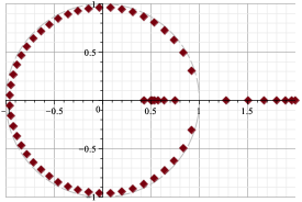
Figure 2. Zeros of the denominator polynomial $Q_{60}$ when the approximated pair is given by $f_{0}(z)=\log\big{(}\frac{z-1}{z-1/a}\big{)}$ and $f_{\infty}(z)=\log\big{(}\frac{z-a}{z-1}\big{)}$ for $a=2$.

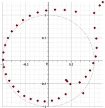
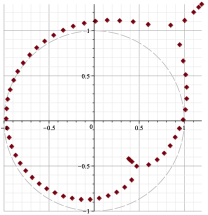
Figure 3. Zeros of the denominator polynomial (a) $Q_{40}$ and (b) $Q_{60}$ when the approximated pair is given by $f_{0}(z)=\log\big{(}\frac{z-1}{z-1/a}\big{)}$ and $f_{\infty}(z)=\log\big{(}\frac{z-a}{z-1}\big{)}$ for $a=1.2+1.3\mathrm{i}$. One can clearly see one zero of $Q_{40}$ not being aligned along Buslaev’s compact $F$.

see Figures 1, 2, and 3.

Figure 1. Buslaev’s compact $F$ for a point $a$ on (a) the imaginary axis (b) the real axis.

Clearly, $F$ separates the plane into two simply connected components, one containing the origin and one containing the point at infinity, which we label by $D_{0}$ and $D_{\infty}$. We shall write

$$F:=F^{\circ}\cup E,\quad E:=\big{\{}a,a^{-1},b,b^{-1}\big{\}},$$

where $F^{\circ}$ consists of four (three when $a$ is real) open disjoint Jordan arcs, see Figure 1. We let $F_{\pm 1}$ (resp. $F_{\pm 1}^{\circ}$) to be closed (resp. open) Jordan arcs connecting $b$ to $b^{-1}$ and containing $\pm 1$, and $F_{a^{\pm 1}}$ (resp. $F_{a^{\pm 1}}^{\circ}$) to be closed (resp. open) Jordan arcs connecting $a^{\pm 1}$ to $b^{\pm 1}$ (we have that $F_{-1}=\varnothing$ when $a\in(-1,0)$ and $F_{1}=\varnothing$ when $a\in(0,1)$). We choose their orientation so that $F_{1}\cup F_{-1}$ is a counterclockwise oriented Jordan curve and $F_{a^{-1}}\cup F_{1}\cup F_{a}$ is a Jordan arc oriented from $a^{-1}$ to $a$, see Figure 1. It is a matter of a simple substitution to see that the set $F^{\circ}$ is comprised of the critical trajectories of the quadratic differential

(3) $$-\frac{(z-b)(z-b^{-1})}{(z-a)(z-a^{-1})}\frac{\mathrm{d}z^{2}}{z^{2}}.$$

From now on we fix $a\in\mathbb{D}\setminus\{0\}$ and the corresponding Buslaev’s compact $F$. In this work we shall be interested in approximating pairs (1) of the form

(4) $$\big{(}f_{\rho|D_{0}},f_{\rho|D_{\infty}}\big{)},\quad f_{\rho}(z):=\frac{1}{2\pi\mathrm{i}}\int_{F}\frac{\rho(s)\mathrm{d}s}{s-z},$$

for some classes of weights $\rho$ to be specified later. Thus, depending on a situation we shall speak about approximants (2) to either a pair of functions or a single function, in both cases referring to (4). As one can clearly see from Figure 1, the structure of the set $F$ is qualitatively different for real and non-real values of $a$. Hence, it should come as no surprise that the description of the asymptotics of the approximants will also depend on whether the parameter $a$ is real or not.

2.1. Asymptotics of the Approximants: $a\in(-1,0)\cup(0,1)$

Recall that in this case $F$ is a union of the unit circle $\mathbb{T}$ and the interval joining $a$ and $a^{-1}$ that we shall denote by $[a^{-1},a]$ (always oriented from $a^{-1}$ to $a$). Let us start by describing the class of weights $\rho$ that we consider. To this end, define

(5) $$w(z)=w(z;a):=\sqrt{(z-a)(z-a^{-1})}$$

to be the branch holomorphic off $[a^{-1},a]$ such that $w(z)=z+\mathcal{O}(1)$ as $z\to\infty$. Given a function $\rho$ on $F$ it will be convenient for us to set

(6) $$h(s):=\rho(s)\left\{\begin{array}[]{rl}w_{\pm}(s),&s\in F_{a^{\pm 1}}^{\circ},\vskip 6.0pt plus 2.0pt minus 2.0pt\\ w(s),&s\in F_{-b}^{\circ},\end{array}\right.$$

where $b:=a/|a|$. We shall say that $\rho\in\mathcal{W}_{1}$ if $h$ extends to a holomorphic and non-vanishing function in some neighborhood of $F\setminus\big{\{}a,a^{-1}\big{\}}$ with the zero increment of the argument along the unit circle and there exist real constants $\alpha,\beta>-1$ such that

(7) $$h_{|(a^{-1},a)}(s)=\widetilde{h}(s)(s-a)^{\alpha+1/2}(s-a^{-1})^{\beta+1/2},$$

where $\widetilde{h}$ is holomorphic and non-vanishing in some neighborhood of $[a^{-1},a]$ and the branches of the power functions are holomorphic across $(a^{-1},a)$. It will also be convenient to single out the following subclass of $\mathcal{W}_{1}$: we shall say that $\rho\in\mathcal{W}_{2}\subset\mathcal{W}_{1}$ if $\alpha=\beta=-1/2$, that is, if $h$ extends to a holomorphic and non-vanishing function in some neighborhood of $F$. In particular, if we define $\rho$ by (6) with $h(s)\equiv 2$, we get that the approximated pair of functions is given by $(1/w,-1/w)$.

For brevity, let us set $\sqrt{x}:=\mathrm{i}\sqrt{|x|}$ when $x<0$. As we shall see below, the $n$-th root behavior of the approximants is described by the following function:

(8) $$\varphi(z):=\frac{z+b+w(z)}{\sqrt{a}+\sqrt{a^{-1}}},$$

which is holomorphic off $[a^{-1},a]$, vanishes at the origin, and has a simple pole at infinity. Moreover, since $w$ has purely imaginary traces on the interval $[a^{-1},a]$ and $w^{2}(e^{\mathrm{i}t})=2e^{\mathrm{i}t}(\cos(t)-\mathfrak{j}(a))$, it can be easily checked that

(9) $$\left\{\begin{array}[]{rl}\varphi_{+}(s)\varphi_{-}(s)=s,&s\in[a^{-1},a],\vskip 6.0pt plus 2.0pt minus 2.0pt\\ |\varphi(s)|=1,&s\in F_{-b}^{\circ}.\end{array}\right.$$

To describe the finer behavior of the approximants let us define the following functions. Let $\log h$ be any smooth continuous branch of the logarithm on the unit circle (recall that $h$ is continuous on $\mathbb{T}$ with the argument that has zero increment). Set

(10) $$D(z):=\exp\left\{\frac{1}{2\pi\mathrm{i}}\int_{\mathbb{T}}\frac{\log h(s)\mathrm{d}s}{s-z}\right\},$$

which is a holomorphic and non-vanishing function off $\mathbb{T}$, that is smooth in the entire plane, and satisfies $D_{+}(s)=D_{-}(s)h(s)$ on the unit circle, see [12, Chapter I]. Therefore, the function

$$\widehat{h}(s):=D^{2}(s)h^{\mp 1}(s),\quad s\in F_{a^{\pm 1}},$$

is non-vanishing and smooth on the interval $(a^{-1},a)$ and admits a continuous determination of its logarithm. Thus, the function

(11) $$S(z):=\exp\left\{\frac{w(z)}{2\pi\mathrm{i}}\int_{[a^{-1},a]}\frac{\log\widehat{h}(s)}{s-z}\frac{\mathrm{d}s}{w_{+}(s)}\right\}$$

is a holomorphic and non-vanishing function off the interval $[a^{-1},a]$ with traces satisfying $S_{+}(s)S_{-}(s)=\widehat{h}(s)$. Given (8), (10), and (11), let us put

(12) $${\mathcal{Q}}_{n}(z):=\left\{\begin{array}[]{rl}(z/\varphi(z))^{n}S(z)/D(z),&z\in D_{0},\vskip 6.0pt plus 2.0pt minus 2.0pt\\ \varphi(z)^{n}D(z)/S(z),&z\in D_{\infty},\end{array}\right.$$

which is a holomorphic and non-vanishing function in $\mathbb{C}\setminus F$ with a pole of order $n$ at infinity and

(13) $${\mathcal{R}}_{n}(z):=\left\{\begin{array}[]{rl}(\varphi(z)/z)^{n}D(z)/S(z),&z\in D_{0},\vskip 6.0pt plus 2.0pt minus 2.0pt\\ -(1/\varphi(z))^{n}S(z)/D(z),&z\in D_{\infty},\end{array}\right.$$

which is a holomorphic and non-vanishing function in $\mathbb{C}\setminus F$ with a zero of multiplicity $n$ at infinity (one can clearly see that ${\mathcal{R}}_{n}$ is essentially a reciprocal of ${\mathcal{Q}}_{n}$ and therefore this definition might appear superfluous, however, for not real $a$ the relation between these two functions will not be as straightforward and we prefer to present the cases of real and non-real parameters in a uniform fashion).

Theorem 1.

Denote by $P_{n}/Q_{n}$ the two-point Padé approximant of type $(n,n+1)$ to (4) with $\rho\in\mathcal{W}_{1}$. Set

(14) $$R_{n}(z):=z^{-n}(Q_{n}f_{\rho}-P_{n})(z),\quad z\in\overline{\mathbb{C}}\setminus F.$$

Then for all $n$ large enough the polynomial $Q_{n}$ has degree $n$ and can be normalized to be monic. In this case, it holds that

(15) $$\left\{\begin{array}[]{rll}Q_{n}&=&\gamma_{n}(1+\upsilon_{{\mathcal{Q}}_{n}}\big{)}{\mathcal{Q}}_{n},\vskip 6.0pt plus 2.0pt minus 2.0pt\\ wR_{n}&=&\gamma_{n}\big{(}1+\upsilon_{{\mathcal{R}}_{n}}\big{)}{\mathcal{R}}_{n},\end{array}\right.$$

locally uniformly in $\overline{\mathbb{C}}\setminus F$, where the error rate functions $\upsilon=\upsilon_{{\mathcal{Q}}_{n}},\upsilon_{{\mathcal{R}}_{n}}$ satisfy

(16) $$|\upsilon(z)|\leq C\left\{\begin{array}[]{ll}1/n,&\rho\in\mathcal{W}_{1},\vskip 6.0pt plus 2.0pt minus 2.0pt\\ c^{n},&\rho\in\mathcal{W}_{2},\end{array}\right.$$

for some constants $C>0$ and $c<1$, and $\gamma_{n}$ is a constant such that the limit $\lim_{z\to\infty}\gamma_{n}{\mathcal{Q}}_{n}(z)z^{-n}=1$ holds.

We can immediately see from (12), (13), and (15) that

(17) $$(f_{\rho}-P_{n}/Q_{n})(z)=\frac{1+o(1)}{w(z)}\left\{\begin{array}[]{rl}(\varphi^{2}(z)/z)^{n}(SD)^{2}(z),&z\in D_{0},\vskip 6.0pt plus 2.0pt minus 2.0pt\\ -(z/\varphi^{2}(z))^{n}/(SD)^{2}(z),&z\in D_{\infty}.\end{array}\right.$$

It further can be deduced from (9) that the right hand side of the above equality is geometrically small in $\overline{\mathbb{C}}\setminus F$.

2.2. Asymptotics of the Approximants: $a\in\mathbb{D}\setminus(-1,1)$

As in the previous subsection, we start by defining the classes of weights $\rho$ we shall consider. We shall say that $\rho\in\mathcal{W}_{1}$ if the restriction of $\rho$ to the arcs $F_{1}^{\circ},F_{-1}^{\circ}$ extends to a holomorphic and non-vanishing function around $F_{1},F_{-1}$; there exist constants $\alpha,\beta>-1$ such that the restriction of $\rho$ to $F_{a}^{\circ},F_{a^{-1}}^{\circ}$ is of the form

(18) $$\widetilde{\rho}(s)(s-a)^{\alpha}(s-a^{-1})^{\beta}$$

where $\widetilde{\rho}$ is holomorphic and non-vanishing around $F_{a},F_{a^{-1}}$ and the branches of the power functions are holomorphic across $F_{a}^{\circ},F_{a^{-1}}^{\circ}$; and

(19) $$\left\{\begin{array}[]{l}\rho_{|F_{a}}(z)+\rho_{|F_{-1}}(z)-\rho_{|F_{1}}(z)\equiv 0,\vskip 6.0pt plus 2.0pt minus 2.0pt\\ \rho_{|F_{a^{-1}}}(z)+\rho_{|F_{-1}}(z)-\rho_{|F_{1}}(z)\equiv 0,\end{array}\right.$$

in some neighborhood of $b$ (upper relation) and in some neighborhood of $b^{-1}$ (lower relation), where, with a slight abuse of notation, we denote by $\rho_{|F_{e}}(z)$ not only the restriction of $\rho$ to $F_{e}$, but also its analytic continuation. Unlike the case of the real parameter, the class $\mathcal{W}_{2}$ will be disjoint from $\mathcal{W}_{1}$. Let now

(20) $$w(z)=w(z;a):=\sqrt{(z-a)(z-a^{-1})(z-b)(z-b^{-1})}$$

be the branch holomorphic in $\mathbb{C}\setminus(F_{a^{-1}}\cup F_{a})$ such that $w(z)=z^{2}+\mathcal{O}(z)$ as $z\to\infty$. We shall say that a function $\rho$ belongs to the class $\mathcal{W}_{2}$ if

(21) $$h(s):=\rho(s)\left\{\begin{array}[]{rl}w_{\pm}(s),&s\in F_{a^{\pm 1}},\vskip 6.0pt plus 2.0pt minus 2.0pt\\ w(s),&s\in F_{-1}^{\circ}\cup F_{1}^{\circ},\end{array}\right.$$

extends to a holomorphic and non-vanishing function in some neighborhood of $F$. It is easy to check that when $h(s)\equiv 2$, we again obtain the pair $(1/w,-1/w)$.

The advantage of class $\mathcal{W}_{2}$ is that the error estimates in the analog of (15) shall be again geometric. However, this class is not very natural as one needs to know the point $b$ explicitly to define functions in this class, however, finding $b$ is in general a transcendental problem. The class $\mathcal{W}_{1}$ is more natural as it for example contains pairs $(c_{0}/w_{a},c_{\infty}/w_{a})$ for some constants $c_{0}\neq\pm c_{\infty}$, where $w_{a}(z):=\sqrt{(z-a)(z-a^{-1})}$ is a branch holomorphic off $F_{a^{-1}}\cup F_{1}\cup F_{a}$.

The analogues of the functions $\varphi$, $D$, and $S$ from (8), (10), and (11) are more complicated now as they need to be defined with the help of various differentials on the Riemann surface

(22) $$\boldsymbol{\mathfrak{S}}:=\left\{\boldsymbol{z}:=(z,w):w^{2}=(z-a)(z-a^{-1})(z-b)(z-b^{-1})\right\},$$

which has genus 1. Moreover, these functions by themselves are not sufficient to define analogs of ${\mathcal{Q}}_{n},{\mathcal{R}}_{n}$. Hence, we opt for a different approach.

The surface $\boldsymbol{\mathfrak{S}}$ can be realized as two copies of $\overline{\mathbb{C}}$ cut along $F_{a^{-1}}\cup F_{a}$ and then glued crosswise along the corresponding arcs. We shall denote these copies by $\boldsymbol{\mathfrak{S}}^{(0)}$ and $\boldsymbol{\mathfrak{S}}^{(1)}$. Denote by $\pi:\boldsymbol{\mathfrak{S}}\to\overline{\mathbb{C}}$ the natural projection $\pi(\boldsymbol{z})=z$. For a point $z\not\in F_{a^{-1}}\cup F_{a}$ we also let $z^{(i)}$ stand for the pull back of $z$ to $\boldsymbol{\mathfrak{S}}^{(i)}$. We put

$$\boldsymbol{\Delta}:=\pi^{-1}(F)=\boldsymbol{\alpha}\cup\boldsymbol{\beta}\cup\boldsymbol{\gamma}\cup\boldsymbol{\delta},$$

where $\boldsymbol{\beta}:=\pi^{-1}(F_{a^{-1}})$ is oriented so that $\boldsymbol{\mathfrak{S}}^{(0)}\setminus\boldsymbol{\Delta}$ remains on the right when it is traversed in the positive direction, $\boldsymbol{\delta}:=\pi^{-1}(F_{a})$ is oriented so that $\boldsymbol{\mathfrak{S}}^{(0)}\setminus\boldsymbol{\Delta}$ remains on the left when it is traversed in the positive direction, and $\boldsymbol{\alpha}:=\pi^{-1}(F_{1})$, $\boldsymbol{\gamma}:=\pi^{-1}(F_{-1})$ are oriented so that their positive directions in $\boldsymbol{\mathfrak{S}}^{(0)}$ coincide with the positive directions of $F_{1}$, $F_{-1}$.

Theorem 2.

Let $h(s)$ be a function on $F$ for which there exist real constants $\alpha(e)$, $e\in E=F\setminus F^{\circ}$, and the branches of $(z-e)^{\alpha(e)}$ such that the product

$$h(s)\prod_{e\in E}(s-e)^{-\alpha(e)}$$

extends to a non-vanishing Hölder continuous function on $F$. Then for each $n\in\mathbb{N}$ there exist a meromorphic in $\boldsymbol{\mathfrak{S}}\setminus\boldsymbol{\Delta}$ function $\Psi_{n}$ and a point $\boldsymbol{z}_{n}\in\boldsymbol{\mathfrak{S}}$ such that

• $\Psi_{n}$ has continuous traces on $\pi^{-1}(F^{\circ})$ that satisfy

  (23) $$\Psi_{n-}(\boldsymbol{s})=\Psi_{n+}(\boldsymbol{s})h(s),\quad\boldsymbol{s}\in\boldsymbol{\Delta};$$

• it has a pole of order $n$ at $\infty^{(1)}$ (of order $n-1$ if $\boldsymbol{z}_{n}=\infty^{(1)}$), a simple pole at $\infty^{(0)}$ (a regular point if $\boldsymbol{z}_{n}=\infty^{(0)}$), a zero of multiplicity $n$ at $0^{(1)}$ (of multiplicity $n+1$ if $\boldsymbol{z}_{n}=0^{(1)}$), a simple zero at $\boldsymbol{z}_{n}\not\in\boldsymbol{\Delta}\cup\{\infty^{(0)},\infty^{(1)},0^{(1)}\}$ (when $\boldsymbol{z}_{n}\in\boldsymbol{\Delta}$ we use explicit representation (48) for $\Psi_{n}$ to treat $\boldsymbol{z}_{n}$ as a zero for both $\Psi_{n+}$ and $\Psi_{n-}$), and otherwise is non-vanishing and finite;

• it holds that

  (24) $$\big{|}\Psi_{n}\big{(}z^{(k)}\big{)}\big{|}^{2}\sim\left\{\begin{array}[]{ll}|z-e|^{(-1)^{1-k}\alpha(e)+m_{n}(e)}&\text{as}\quad z\to e\in\{a,a^{-1}\},\vskip 6.0pt plus 2.0pt minus 2.0pt\\ |z-e|^{(-1)^{1-k}\alpha(e)+m_{n}(e)}&\text{as}\quad D_{0}\ni z\to e\in\{b,b^{-1}\},\vskip 6.0pt plus 2.0pt minus 2.0pt\\ |z-e|^{(-1)^{k}\alpha(e)+m_{n}(e)}&\text{as}\quad D_{\infty}\ni z\to e\in\{b,b^{-1}\},\end{array}\right.$$

  for $k\in\{0,1\}$, where $m_{n}(e):=1$ when $\pi(\boldsymbol{z}_{n})=e$ and $m_{n}(e):=0$ otherwise.

Conversely, if $\Psi$ is a function with a zero of multiplicity at least $n$ at $0^{(1)}$, a pole of order at most $n$ at $\infty^{(1)}$, at most a simple pole at $\infty^{(0)}$, and no other poles, and if it satisfies (23) and

$$\big{|}\Psi_{n}\big{(}z^{(k)}\big{)}\big{|}^{2}=\left\{\begin{array}[]{ll}\mathcal{O}\big{(}|z-e|^{(-1)^{1-k}\alpha(e)}\big{)}&\text{as}\quad z\to e\in\{a,a^{-1}\},\vskip 6.0pt plus 2.0pt minus 2.0pt\\ \mathcal{O}\big{(}|z-e|^{(-1)^{1-k}\alpha(e)}\big{)}&\text{as}\quad D_{0}\ni z\to e\in\{b,b^{-1}\},\vskip 6.0pt plus 2.0pt minus 2.0pt\\ \mathcal{O}\big{(}|z-e|^{(-1)^{k}\alpha(e)}\big{)}&\text{as}\quad D_{\infty}\ni z\to e\in\{b,b^{-1}\},\end{array}\right.$$

then $\Psi$ a constant multiple of $\Psi_{n}$.

As mentioned before, the functions $\Psi_{n}$ can be explicitly expressed via various differential on $\boldsymbol{\mathfrak{S}}$ as well as Riemann’s theta functions, see (48) further below.

In our asymptotic analysis we shall be interested only in the indices $n$ for which points $\boldsymbol{z}_{n}$ stay away from $\infty^{(1)}$. As stated in the following proposition, there are infinitely many such indices.

Proposition 3.

Given $\varepsilon>0$, let $D_{\varepsilon}(z)$ be a disk of radius $\varepsilon$ in the spherical metric around $z\in\overline{\mathbb{C}}$ and $D_{\varepsilon}(\boldsymbol{z})$ be the connected component of $\pi^{-1}(D_{\varepsilon}(z))$ containing $\boldsymbol{z}$. Define

(25) $$\mathbb{N}_{\varepsilon}:=\left\{n\in\mathbb{N}:\boldsymbol{z}_{n}\not\in D_{\varepsilon}\big{(}\infty^{(1)}\big{)}\right\}.$$

Then for all $\varepsilon$ small enough either $n$ or $n-1$ belongs to $\mathbb{N}_{\varepsilon}$.

In accordance with our notation, let us put $B^{(i)}:=\pi^{-1}(B)\cap\boldsymbol{\mathfrak{S}}^{(i)}$ for any set $B$. Now we are ready to define the analogues of (12) and (13) for non-real $a$. Set

(26) $${\mathcal{Q}}_{n}(z):=\left\{\begin{array}[]{rl}\Psi_{n|D_{0}^{(0)}}(\boldsymbol{z}),&z\in D_{0},\vskip 6.0pt plus 2.0pt minus 2.0pt\\ \Psi_{n|D_{\infty}^{(1)}}(\boldsymbol{z}),&z\in D_{\infty},\end{array}\right.$$

which is a sectionally holomorphic function in $\mathbb{C}\setminus F$ with a pole of order $n$ at infinity, and put

(27) $${\mathcal{R}}_{n}(z):=\frac{1}{z^{n}}\left\{\begin{array}[]{rl}\Psi_{n|D_{0}^{(1)}}(\boldsymbol{z}),&z\in D_{0},\vskip 6.0pt plus 2.0pt minus 2.0pt\\ -\Psi_{n|D_{\infty}^{(0)}}(\boldsymbol{z}),&z\in D_{\infty},\end{array}\right.$$

which is also a sectionally holomorphic function in $\overline{\mathbb{C}}\setminus F$ with a zero of multiplicity $n-1$ at infinity. Due to the specifics of the Riemann-Hilbert analysis, which is used to study the behavior of the Padé approximants, we shall also need the following functions. Let $\Upsilon_{n}$ be a rational function on $\boldsymbol{\mathfrak{S}}$ that is finite except for two simple poles at $\infty^{(0)}$ and $\boldsymbol{z}_{n}$, and has a simple zero at $0^{(1)}$ (such a function is unique up to a scalar factor). Set

$$\Psi_{n}^{\star}:=\Psi_{n}\Upsilon_{n}$$

and define ${\mathcal{Q}}_{n}^{\star}$ and ${\mathcal{R}}_{n}^{\star}$ via (26) and (27), respectively, with $\Psi_{n}$ replaced by $\Psi_{n}^{\star}$ and $z^{n}$ replaced by $z^{n+1}$ in (27). These functions are holomorphic in $\mathbb{C}\setminus F$, ${\mathcal{Q}}_{n}^{\star}$ has a pole of order $n$ at infinity while ${\mathcal{R}}_{n}^{\star}$ has a zero of multiplicity $n-1$ there.

Theorem 4.

Denote by $P_{n}/Q_{n}$ the two-point Padé approximant of type $(n,n+1)$ to (4) with $\rho\in\mathcal{W}_{1}\cup\mathcal{W}_{2}$ and let $R_{n}$ be given by (14). Further, let ${\mathcal{Q}}_{n}$ and ${\mathcal{R}}_{n}$ be given by (26) and (27) for $\Psi_{n}$ defined as in Theorem 2 with $h$ given by (21). Then for any $\varepsilon>0$ and all $n\in\mathbb{N}_{\varepsilon}$ large enough the polynomial $Q_{n}$ has degree $n$ and can be normalized to be monic. In this case, it holds that

(28) $$\left\{\begin{array}[]{rll}Q_{n}&=&\gamma_{n}\left[\big{(}1+\upsilon_{n1}\big{)}{\mathcal{Q}}_{n}+\upsilon_{n2}\mathcal{Q}_{n-1}^{\star}\right],\vskip 6.0pt plus 2.0pt minus 2.0pt\\ wR_{n}&=&\gamma_{n}\left[\big{(}1+\upsilon_{n1}\big{)}{\mathcal{R}}_{n}+\upsilon_{n2}\mathcal{R}_{n-1}^{\star}\right],\end{array}\right.$$

locally uniformly in $\overline{\mathbb{C}}\setminus F$, where $\gamma_{n}$ is a constant such that $\lim_{z\to\infty}\gamma_{n}{\mathcal{Q}}_{n}(z)z^{-n}=1$ and the functions $\upsilon=\upsilon_{nj}$ satisfy (16).

Similarly to (17) we have that

$$f_{\rho}-\frac{P_{n}}{Q_{n}}=\frac{z^{n}{\mathcal{R}}_{n}}{w{\mathcal{Q}}_{n}}\frac{1+\upsilon_{n,1}+\upsilon_{n,2}(\mathcal{R}_{n-1}^{\star}/{\mathcal{R}}_{n})}{1+\upsilon_{n,1}+\upsilon_{n,2}(\mathcal{Q}_{n-1}^{\star}/{\mathcal{Q}}_{n})}.$$

Due to the presence of a floating zero $\boldsymbol{z}_{n}$, the above formula does not immediately imply the locally uniform convergence of the approximants to $f_{\rho}$. Indeed, when

$$\boldsymbol{z}_{n}\in D_{\mathcal{R}}:=D_{0}^{(1)}\cup D_{\infty}^{(0)},$$

it holds that ${\mathcal{R}}_{n}(z_{n})=0$, which yields that the approximant has an additional interpolation point near $z_{n}$. However, when

$$\boldsymbol{z}_{n}\in D_{\mathcal{Q}}:=D_{0}^{(0)}\cup D_{\infty}^{(1)},$$

it holds that ${\mathcal{Q}}_{n}(z_{n})=0$ and therefore the approximant has pole in a vicinity of $z_{n}$. The following results help us further elucidate the situation.

Theorem 5.

The functions $\Psi_{n}$ can be normalized so that for any closed set $B\subset\overline{\mathbb{C}}\setminus F$ and any $\delta>0$ there exist positive constants $C(B)$ and $C_{\delta}(B)$ such that

(29) $$|{\mathcal{Q}}_{n}(z)|e^{-ng(z)}\left\{\begin{array}[]{ll}\leq C(B),&z\in B,\vskip 6.0pt plus 2.0pt minus 2.0pt\\ \geq C_{\delta}(B),&z\in B\setminus\pi\big{(}D_{\mathcal{Q}}\cap D_{\delta}(\boldsymbol{z}_{n})\big{)},\end{array}\right.$$

where $g(z)$ is a continuous function in $\mathbb{C}$ that is harmonic in $\mathbb{C}\setminus F$ and satisfies

(30) $$g(z)=\log|z|+\mathcal{O}(1),\quad z\to\infty,\quad\text{and}\quad 2g(s)=\log|s|,\quad s\in F$$

(it follows from the minimum principle for superharmonic functions that $2g(z)-\log|z|>0$ in $\mathbb{C}\setminus F$). Moreover, the constants $C(B)$ and $C_{\delta}(B)$ can be adjusted so that

(31) $$|{\mathcal{R}}_{n}(z)|e^{(n-1)g(z)}\left\{\begin{array}[]{ll}\leq C(B),&z\in B,\vskip 6.0pt plus 2.0pt minus 2.0pt\\ \geq C_{\delta}(B),&z\in B\setminus\pi\big{(}D_{\mathcal{R}}\cap D_{\delta}(\boldsymbol{z}_{n})\big{)}.\end{array}\right.$$

The functions $\Upsilon_{n}$ can be normalized so that inequalities (29) and (31) hold for ${\mathcal{Q}}_{n}^{\star}$ and ${\mathcal{R}}_{n}^{\star}$ as well. Moreover, for any $\delta>0$ there exists a constant $C_{\delta}$ such that

(32) $$C_{\delta}\geq\left\{\begin{array}[]{ll}|\mathcal{Q}_{n-1}^{\star}/{\mathcal{Q}}_{n}|&\text{in}\quad\overline{\mathbb{C}}\setminus\pi\big{(}\overline{D}_{\mathcal{Q}}\cap D_{\delta}(\boldsymbol{z}_{n})\big{)},\vskip 6.0pt plus 2.0pt minus 2.0pt\\ |\mathcal{R}_{n-1}^{\star}/{\mathcal{R}}_{n}|&\text{in}\quad\overline{\mathbb{C}}\setminus\left(D_{\delta}(\infty)\cup\pi\big{(}\overline{D}_{\mathcal{R}}\cap D_{\delta}(\boldsymbol{z}_{n})\big{)}\right).\end{array}\right.$$

In view of Buslaev’s theorem, it should be clear that $2g(z)-\log|z|=g_{F}(z,0)+g_{F}(z,\infty)$.

The author would like to thank Andrei Martínez Finkelshtein for many valuable discussions.

3. Proof of Theorems 2, 5 and Proposition 3

Let $\boldsymbol{\mathfrak{S}}$ be the Riemann surface defined in (22). We consider each $\boldsymbol{\mathfrak{S}}^{(i)}$ to be closed subsets of $\boldsymbol{\mathfrak{S}}$, i.e., it does contain cycles $\boldsymbol{\beta},\boldsymbol{\delta}$. We define the conformal involution on $\boldsymbol{\mathfrak{S}}$ by $\boldsymbol{z}=(z,w)\mapsto\boldsymbol{z}^{*}=(z,-w)$. It is easy to see that the pair $(\boldsymbol{\alpha},\boldsymbol{\beta})$ forms a homology basis on $\boldsymbol{\mathfrak{S}}$. In particular, $\boldsymbol{\mathfrak{S}}_{\boldsymbol{\alpha},\boldsymbol{\beta}}:=\boldsymbol{\mathfrak{S}}\setminus(\boldsymbol{\alpha}\cup\boldsymbol{\beta})$ is simply connected.

3.1. Nuttall’s Differential

Let $w(\boldsymbol{z}):=(-1)^{i}w(z)$, $\boldsymbol{z}\in\boldsymbol{\mathfrak{S}}^{(i)}$, where $w(z)$ is the branch defined in (20). For convenience, set

$$v(\boldsymbol{z}):=\frac{(z-b)(z-b^{-1})}{w(\boldsymbol{z})}$$

and $v(z):=v(\boldsymbol{z})$ for $\boldsymbol{z}\in\boldsymbol{\mathfrak{S}}^{(0)}\setminus\{\boldsymbol{\beta}\cup\boldsymbol{\gamma}\cup\boldsymbol{\delta}\}$. Notice that $v(0)=v(\infty)=1$. The differential

(33) $$\mathcal{N}(\boldsymbol{s})=\frac{1-v(\boldsymbol{s})}{2s}\mathrm{d}s$$

is holomorphic except for two simple poles at $0^{(1)}$ and $\infty^{(1)}$ with respective residues $1$ and $-1$. Moreover, one can readily check using (3) that all the periods of $\mathcal{N}(\boldsymbol{s})$ are purely imaginary and therefore we can define

(34) $$\omega:=-\frac{1}{2\pi\mathrm{i}}\oint_{\boldsymbol{\beta}}\mathcal{N}\quad\text{and}\quad\tau:=\frac{1}{2\pi\mathrm{i}}\oint_{\boldsymbol{\alpha}}\mathcal{N},$$

which are clearly real constants.

Lemma 6.

Let $\sqrt{a}$ be the principal value of the square root. Define

(35) $$\Phi(\boldsymbol{z}):=\sqrt{a}\exp\left\{\int_{\boldsymbol{a}}^{\boldsymbol{z}}\mathcal{N}\right\},\quad\boldsymbol{z}\in\boldsymbol{\mathfrak{S}}_{\boldsymbol{\alpha},\boldsymbol{\beta}},$$

where the path of integration belongs entirely to $\boldsymbol{\mathfrak{S}}_{\boldsymbol{\alpha},\boldsymbol{\beta}}$. The function $\Phi(\boldsymbol{z})$ is holomorphic and non-vanishing in $\boldsymbol{\mathfrak{S}}_{\boldsymbol{\alpha},\boldsymbol{\beta}}\setminus\big{\{}\infty^{(1)},0^{(1)}\big{\}}$ with a simple pole at $\infty^{(1)}$ and a simple zero at $0^{(1)}\in\boldsymbol{\mathfrak{S}}^{(1)}$. It holds that $\Phi(\boldsymbol{z})\Phi(\boldsymbol{z}^{*})=z$ and the traces of $\Phi(\boldsymbol{z})$ satisfy

(36) $$\Phi_{+}=\Phi_{-}\left\{\begin{array}[]{lll}\exp\left\{2\pi\mathrm{i}\tau\right\}&\text{on}&\boldsymbol{\beta},\vskip 6.0pt plus 2.0pt minus 2.0pt\\ \exp\left\{2\pi\mathrm{i}\omega\right\}&\text{on}&\boldsymbol{\alpha}.\end{array}\right.$$

Moreover, $|\Phi(\boldsymbol{z})|^{2}<|z|$ for $z\in D_{\mathcal{R}}$ and $|\Phi(\boldsymbol{z})|^{2}>|z|$ for $z\in D_{\mathcal{Q}}$.

Proof.

The holomorphy properties of $\Phi$ follow immediately from the corresponding properties of $\mathcal{N}$. Since $v(\boldsymbol{z})=-v(z)$ for $\boldsymbol{z}\in\boldsymbol{\mathfrak{S}}^{(1)}\setminus\{\boldsymbol{\beta}\cup\boldsymbol{\gamma}\}$, it holds that

(37) $$\Phi(\boldsymbol{z})\Phi(\boldsymbol{z}^{*})=a\exp\left\{\int_{a}^{z}\frac{(1-v(t))\mathrm{d}t}{2t}+\int_{a}^{z}\frac{(1+v(t))\mathrm{d}t}{2t}\right\}=a\exp\left\{\int_{a}^{z}\frac{\mathrm{d}t}{t}\right\}=z.$$

Furthermore, we get on $\boldsymbol{\alpha}$ and $\boldsymbol{\beta}$ that

$$\Phi_{+}=\Phi_{-}\exp\left\{-\oint_{\boldsymbol{\beta}}\mathcal{N}\right\}\quad\text{and}\quad\Phi_{+}=\Phi_{-}\exp\left\{\oint_{\boldsymbol{\alpha}}\mathcal{N}\right\},$$

respectively, which yields (36), see (34). Finally, recall that $F$ consists of the critical trajectories of the quadratic differential $-(v(z)\mathrm{d}z/z)^{2}$, see (3). Hence, the integral of $v(t)\mathrm{d}t/t$ on any subarc of $F$ is purely imaginary and therefore

$$\big{|}\Phi^{2}(\boldsymbol{s})\big{|}=|s|\exp\left\{\pm\mathrm{Re}\left(\int_{a}^{s}\frac{v(t)}{t}\mathrm{d}t\right)\right\}=|s|,\quad\boldsymbol{s}\in\boldsymbol{\Delta},$$

where the sign $-$ is used if $\boldsymbol{s}\in\boldsymbol{\mathfrak{S}}^{(0)}$ and the sign $+$ is used if $\boldsymbol{s}\in\boldsymbol{\mathfrak{S}}^{(1)}$. The last conclusion of the lemma now follows from the maximum modulus principle. ∎

3.2. Holomorphic Differentials

It can be readily checked that

$$\mathcal{H}(\boldsymbol{s}):=\frac{C\mathrm{d}s}{w(\boldsymbol{s})},\quad C:=\left(\oint_{\boldsymbol{\alpha}}\frac{\mathrm{d}s}{w(\boldsymbol{s})}\right)^{-1},\quad\mathbf{B}:=\oint_{\boldsymbol{\beta}}\mathcal{H},$$

is a holomorphic differential on $\boldsymbol{\mathfrak{S}}$ (unique up to a multiplicative constant). It is also known that $\mathrm{Im}(\mathbf{B})>0$. The proof of the following lemma is absolutely analogous to the proof of Lemma 6.

Lemma 7.

Given a constant $\sigma\in\mathbb{C}$, define

(38) $$A_{\sigma}(z):=\exp\left\{-2\pi\mathrm{i}\sigma\int_{\boldsymbol{a}}^{\boldsymbol{z}}\mathcal{H}\right\},\quad\boldsymbol{z}\in\boldsymbol{\mathfrak{S}}_{\boldsymbol{\alpha},\boldsymbol{\beta}},$$

where the path of integration belongs entirely to $\boldsymbol{\mathfrak{S}}_{\boldsymbol{\alpha},\boldsymbol{\beta}}$. The function $A_{\sigma}(\boldsymbol{z})$ is holomorphic and non-vanishing in $\boldsymbol{\mathfrak{S}}_{\boldsymbol{\alpha},\boldsymbol{\beta}}$. It holds that $A_{\sigma}(\boldsymbol{z})A_{\sigma}(\boldsymbol{z}^{*})\equiv 1$ and the traces of $A_{\sigma}(\boldsymbol{z})$ on $\boldsymbol{\alpha},\boldsymbol{\beta}$ satisfy

(39) $$A_{\sigma+}=A_{\sigma-}\left\{\begin{array}[]{rll}\exp\left\{-2\pi\mathrm{i}\sigma\right\}&\text{on}&\boldsymbol{\beta},\vskip 6.0pt plus 2.0pt minus 2.0pt\\ \exp\left\{2\pi\mathrm{i}\mathbf{B}\sigma\right\}&\text{on}&\boldsymbol{\alpha}.\end{array}\right.$$

3.3. Cauchy’s Differential

Denote by $\mathcal{C}_{\boldsymbol{z}}$ the unique meromorphic differential that has two simple poles at $\boldsymbol{z}$ and $\boldsymbol{z}^{*}$ with residues $1$ and $-1$, respectively, and whose $\boldsymbol{\alpha}$-period is zero. When $\pi(\boldsymbol{z})\in\mathbb{C}$, one can readily check that

(40) $$\mathcal{C}_{\boldsymbol{z}}(\boldsymbol{s})=\frac{w(\boldsymbol{z})}{s-z}\frac{\mathrm{d}s}{w(\boldsymbol{s})}-\left(\oint_{\boldsymbol{\alpha}}\frac{w(\boldsymbol{z})}{s-z}\frac{\mathrm{d}s}{w(\boldsymbol{s})}\right)\mathcal{H}(\boldsymbol{s}).$$

Lemma 8.

Let $h(z)$ be as in Theorem 2. Fix a smooth determination of

$$\log h(s)-\sum_{e\in E}\alpha(e)\log(z-e)$$

on each of the arcs $F_{a},F_{a^{-1}},F_{1},F_{-1}$. Define $\lambda_{h}(\boldsymbol{s}):=-\log h(s)$, $s\in F^{\circ}$, and

(41) $$S_{h}(\boldsymbol{z}):=\exp\left\{\frac{1}{4\pi\mathrm{i}}\oint_{\boldsymbol{\Delta}}\lambda_{h}\mathcal{C}_{\boldsymbol{z}}\right\},\quad\boldsymbol{z}\in\boldsymbol{\mathfrak{S}}\setminus\boldsymbol{\Delta}.$$

The function $S_{h}(\boldsymbol{z})$ is holomorphic and non-vanishing in $\boldsymbol{\mathfrak{S}}\setminus\boldsymbol{\Delta}$. It holds that $S_{h}(\boldsymbol{z})S_{h}(\boldsymbol{z}^{*})\equiv 1$ and the traces of $S_{h}(\boldsymbol{z})$ satisfy

(42) $$S_{h+}(\boldsymbol{s})=\frac{S_{h-}(\boldsymbol{s})}{h(s)}\left\{\begin{array}[]{rcl}1,&\text{on}&\boldsymbol{\Delta}\setminus\boldsymbol{\alpha},\vskip 6.0pt plus 2.0pt minus 2.0pt\\ \exp\big{\{}-\oint_{\boldsymbol{\Delta}}\lambda_{h}\mathcal{H}\big{\}},&\text{on}&\boldsymbol{\alpha},\end{array}\right.$$

where the points of self-intersection need to be excluded. Moreover, it holds that

(43) $$\big{|}S_{h}\big{(}z^{(k)}\big{)}\big{|}^{2}\sim\left\{\begin{array}[]{ll}|z-e|^{(-1)^{1-k}\alpha(e)}&\text{as}\quad z\to e\in\{a,a^{-1}\},\vskip 6.0pt plus 2.0pt minus 2.0pt\\ |z-e|^{(-1)^{1-k}\alpha(e)}&\text{as}\quad D_{0}\ni z\to e\in\{b,b^{-1}\},\vskip 6.0pt plus 2.0pt minus 2.0pt\\ |z-e|^{(-1)^{k}\alpha(e)}&\text{as}\quad D_{\infty}\ni z\to e\in\{b,b^{-1}\},\end{array}\right.\quad k\in\{0,1\}.$$

Proof.

Let $\boldsymbol{\nu}$ be an involution-symmetric cycle on $\boldsymbol{\mathfrak{S}}$ passing through ramification points $\boldsymbol{p}_{1},\boldsymbol{p}_{2}$ and $\lambda_{\boldsymbol{\nu}}$ be an involution-symmetric function on $\boldsymbol{\nu}$ such that

$$\lambda_{\boldsymbol{\nu}}(\boldsymbol{z})+\alpha_{1}\log(z-p_{1})+\alpha_{2}\log(z-p_{2})$$

is Hölder smooth on $\boldsymbol{\nu}$ for some real constants $\alpha_{1},\alpha_{2}$, where the determinations of the logarithms are holomorphic across $\pi(\boldsymbol{\nu})\setminus\{p_{1},p_{2}\}$. Set

$$\Lambda_{\boldsymbol{\nu}}(\boldsymbol{z}):=\frac{1}{4\pi\mathrm{i}}\oint_{\boldsymbol{\nu}}\lambda_{\boldsymbol{\nu}}\mathcal{C}_{\boldsymbol{z}}.$$

Since $\mathcal{C}_{\boldsymbol{z}^{*}}=-\mathcal{C}_{\boldsymbol{z}}$, it holds that $\Lambda_{\boldsymbol{\nu}}(\boldsymbol{z})+\Lambda_{\boldsymbol{\nu}}(\boldsymbol{z}^{*})\equiv 0$. Moreover, it is known [24, Eq. (2.7)–(2.9)] that $\Lambda_{\boldsymbol{\nu}}(\boldsymbol{z})$ is a holomorphic function in $\boldsymbol{\mathfrak{S}}\setminus(\boldsymbol{\nu}\cup\boldsymbol{\alpha})$ with continuous traces on $(\boldsymbol{\nu}\setminus\boldsymbol{\alpha})\setminus\{\boldsymbol{p}_{1},\boldsymbol{p}_{2}\}$ and $(\boldsymbol{\alpha}\setminus\boldsymbol{\nu})\setminus\{\boldsymbol{p}_{1},\boldsymbol{p}_{2}\}$ that satisfy

$$\Lambda_{\boldsymbol{\nu}+}(\boldsymbol{s})-\Lambda_{\boldsymbol{\nu}-}(\boldsymbol{s})=\left\{\begin{array}[]{rl}\lambda_{\boldsymbol{\nu}}(\boldsymbol{s}),&\boldsymbol{s}\in\boldsymbol{\nu}\setminus\boldsymbol{\alpha},\vskip 6.0pt plus 2.0pt minus 2.0pt\\ -\oint_{\boldsymbol{\nu}}\lambda_{\boldsymbol{\nu}}\mathcal{H},&\boldsymbol{s}\in\boldsymbol{\alpha}\setminus\boldsymbol{\nu},\end{array}\right.$$

where we used the fact that $\lambda_{\boldsymbol{\nu}}(\boldsymbol{s})=\lambda_{\boldsymbol{\nu}}(\boldsymbol{s}^{*})$ and the jumps need to be added up on subarcs of $\boldsymbol{\nu}\cap\boldsymbol{\alpha}$. In the absence of logarithmic singularities, i.e., when all $\alpha(e)=0$, the claims of the lemma now follow by summing up $\Lambda_{\boldsymbol{\nu}}$ over all $\boldsymbol{\nu}\in\{\boldsymbol{\alpha},\boldsymbol{\beta},\boldsymbol{\gamma},\boldsymbol{\delta}\}$ while taking $\lambda_{\boldsymbol{\nu}}:=\lambda_{h|\boldsymbol{\nu}}$.

Let $\Lambda:=\sum_{\boldsymbol{\nu}=\boldsymbol{\alpha},\boldsymbol{\beta},\boldsymbol{\gamma},\boldsymbol{\delta}}\Lambda_{\boldsymbol{\nu}}$. When a branch point $\boldsymbol{p}$ is such that $\pi(\boldsymbol{p})\in\{a,a^{-1}\}$, there is exactly one cycle from the chain $\boldsymbol{\Delta}$ passing through $\boldsymbol{p}$ (either $\boldsymbol{\beta}$ or $\boldsymbol{\delta}$). Moreover, since $\boldsymbol{\beta}$ and $\boldsymbol{\delta}$ separate $\boldsymbol{\mathfrak{S}}$ into the sheets $\boldsymbol{\mathfrak{S}}^{(0)}\setminus\{\boldsymbol{\beta}\cup\boldsymbol{\delta}\}$ and $\boldsymbol{\mathfrak{S}}^{(1)}\setminus\{\boldsymbol{\beta}\cup\boldsymbol{\delta}\}$, the analysis of [1, Section 5.2] applies and yields that

$$\Lambda\big{(}z^{(k)}\big{)}=(-1)^{1-k}\frac{\alpha(p)}{2}\log(p-z)+\mathcal{O}(1)\quad\text{as}\quad z\to p\in\big{\{}a,a^{-1}\big{\}},$$

for $k\in\{0,1\}$, where $\log(p-\cdot)$ is holomorphic in some neighborhood of $p=a$ cut along $F_{p}$. The situation when $p\in\{b,b^{-1}\}$ is again very similar to the one discussed in [1, Section 5.2]. Clearly, the singular behavior around $p$ comes from the first term in (40). As explained in [12, Section I.8.5], to understand this behavior it is enough to find a function that has logarithmic singularity at $p$ and the same jumps across the cycles comprising $\boldsymbol{\Delta}$. Thus, it can be checked that

$$\Lambda\big{(}z^{(k)}\big{)}=\pm(-1)^{1-k}\frac{\alpha(p)}{2}\log(z-p)+\mathcal{O}(1)\quad\text{as}\quad z\to p\in\big{\{}b,b^{-1}\big{\}},$$

where the sign $+$ is used if $z\in D_{0}$ and the sign $-$ is used if $z\in D_{\infty}$, and $\log(\cdot-p)$ has a jump along $F_{a}$ when $p=b$ and $F_{a^{-1}}$ when $p=b^{-1}$. ∎

3.4. Jacobi Inversion Problem

We define Abel’s map on $\boldsymbol{\mathfrak{S}}$ by

$$\mathfrak{a}(\boldsymbol{z}):=\int_{\boldsymbol{a}}^{\boldsymbol{z}}\mathcal{H},\quad\boldsymbol{z}\in\boldsymbol{\mathfrak{S}}_{\boldsymbol{\alpha},\boldsymbol{\beta}},$$

where the path of integration lies entirely in $\boldsymbol{\mathfrak{S}}_{\boldsymbol{\alpha},\boldsymbol{\beta}}$, and set $\mathfrak{a}(\boldsymbol{z}):=\mathfrak{a}_{+}(\boldsymbol{z})$ when $\boldsymbol{z}\in\boldsymbol{\alpha}\cup\boldsymbol{\beta}$. Since $\boldsymbol{\mathfrak{S}}$ has genus $1$, any Jacobi inversion problem is uniquely solvable on $\boldsymbol{\mathfrak{S}}$. In particular, given a function $h$ and an integer $n\in\mathbb{N}$, there exist unique $\boldsymbol{z}_{n}=\boldsymbol{z}_{n}(h)\in\boldsymbol{\mathfrak{S}}$ and $j_{n},m_{n}\in\mathbb{Z}$ such that

(44) $$\mathfrak{a}(\boldsymbol{z}_{n})=\mathfrak{a}\big{(}\infty^{(0)}\big{)}-\frac{1}{2\pi\mathrm{i}}\oint_{\boldsymbol{\Delta}}\lambda_{h}\mathcal{H}+n(\omega+\mathbf{B}\tau)+j_{n}+\mathbf{B}m_{n}.$$

Lemma 9.

For $\varepsilon>0$, let $\mathbb{N}_{\varepsilon}$ be defined by (25). Then the conclusions of Proposition 3 hold true. Further, let $\boldsymbol{z}_{n}^{\star}=\boldsymbol{z}_{n}^{\star}(h)$ be the solution of the following Jacobi inversion problem:

$$\mathfrak{a}\big{(}\boldsymbol{z}_{n}^{\star}+0^{(1)}-\boldsymbol{z}_{n}-\infty^{(0)}\big{)}\in\mathbb{Z}+\mathbf{B}\mathbb{Z}.$$

Then there exists a domain $U_{\varepsilon}\ni\infty^{(0)}$ such that $\boldsymbol{z}_{n-1}^{\star}\not\in U_{\varepsilon}$ for all $n\in\mathbb{N}_{\varepsilon}$.

Proof.

According to Riemann’s relations, it holds that

$$\mathfrak{a}\big{(}\infty^{(1)}\big{)}-\mathfrak{a}\big{(}0^{(1)}\big{)}=\int_{0^{(1)}}^{\infty^{(1)}}\mathcal{H}=\frac{1}{2\pi\mathrm{i}}\oint_{\boldsymbol{\beta}}\mathcal{M}_{\infty^{(1)},0^{(1)}},$$

where $\mathcal{M}_{\boldsymbol{z}_{1},\boldsymbol{z}_{2}}$ is a meromorphic differential having two simple poles at $\boldsymbol{z}_{1}$ and $\boldsymbol{z}_{2}$ with residues $1$ and $-1$, respectively, and zero period on $\boldsymbol{\alpha}$. In fact,

$$\mathcal{M}_{\infty^{(1)},0^{(1)}}=-\mathcal{N}+2\pi\mathrm{i}\tau\mathcal{H}$$

as one can see from (34). That is, it holds that

$$\mathfrak{a}\big{(}\infty^{(1)}\big{)}-\mathfrak{a}\big{(}0^{(1)}\big{)}=-\frac{1}{2\pi\mathrm{i}}\oint_{\boldsymbol{\beta}}\mathcal{N}+\tau\oint_{\boldsymbol{\beta}}\mathcal{H}=\omega+\mathbf{B}\tau.$$

It also follows from (44) that

$$\mathfrak{a}(\boldsymbol{z}_{n})-\mathfrak{a}(\boldsymbol{z}_{n-1})-(\omega+\mathbf{B}\tau)\in\mathbb{Z}+\mathbf{B}\mathbb{Z}.$$

The continuity of $\mathfrak{a}(\boldsymbol{z})$ and the unique solvability of the Jacobi inversion problem now yield that if $\boldsymbol{z}_{n}\to\infty^{(1)}$ along some subsequence $\mathbb{N}^{\prime}$, then $\boldsymbol{z}_{n-1}\to 0^{(1)}$ as $\mathbb{N}^{\prime}\ni n\to\infty$, which proves unboundedness of $\mathbb{N}_{\varepsilon}$ as well as the fact that either $n$ or $n-1$ is in $\mathbb{N}_{\varepsilon}$ for all $\varepsilon$ small enough. The same argument proves the last claim of the lemma since $\boldsymbol{z}_{n-1}^{\star}\to\infty^{(0)}$ along some subsequence implies that $\boldsymbol{z}_{n-1}\to 0^{(1)}$ and respectively $\boldsymbol{z}_{n}\to\infty^{(1)}$ along the same subsequence. ∎

3.5. Riemann’s Theta Function

Recall that the theta function associated with $\mathbf{B}$ is an entire transcendental function defined by

$$\theta(u):=\sum_{n\in\mathbb{Z}}\exp\bigg{\{}\pi\mathrm{i}\mathbf{B}n^{2}+2\pi\mathrm{i}un\bigg{\}},\quad u\in\mathbb{C}.$$

Lemma 10.

Let $h$ and $\boldsymbol{z}_{n}$ be as above. Define

(45) $$\Theta_{n}(\boldsymbol{z}):=\frac{\theta\left(\mathfrak{a}(\boldsymbol{z})-\mathfrak{a}(\boldsymbol{z}_{n})-\frac{1+\mathbf{B}}{2}\right)}{\theta\left(\mathfrak{a}(\boldsymbol{z})-\mathfrak{a}\big{(}\infty^{(0)}\big{)}-\frac{1+\mathbf{B}}{2}\right)}.$$

The function $\Theta_{n}$ is meromorphic in $\boldsymbol{\mathfrak{S}}_{\boldsymbol{\alpha},\boldsymbol{\beta}}$ with a simple zero at $\boldsymbol{z}_{n}$, a simple pole at $\infty^{(0)}$, and otherwise non-vanishing and finite. In fact, it is holomorphic across $\boldsymbol{\beta}$ and

(46) $$\Theta_{n+}=\Theta_{n-}\exp\left\{\oint_{\boldsymbol{\Delta}}\lambda_{h}\mathcal{H}-2\pi\mathrm{i}n(\tau+\mathbf{B}\omega)-2\pi\mathrm{i}\mathbf{B}m_{n}\right\}\quad\text{on}\quad\boldsymbol{\alpha}.$$

Proof.

It can be directly checked that

(47) $$\theta(u+j+\mathbf{B}m)=\exp\big{\{}-\pi\mathrm{i}\mathbf{B}m^{2}-2\pi\mathrm{i}um\big{\}}\theta(u),\quad j,m\in\mathbb{Z}.$$

Moreover, it is known that $\theta(u)=0$ if and only if $u=(1+\mathbf{B})/2+j+\mathbf{B}m$, $j,m\in\mathbb{Z}$. Further, recall that

$$\mathfrak{a}_{+}-\mathfrak{a}_{-}=\left\{\begin{array}[]{rcl}-\oint_{\boldsymbol{\beta}}\mathcal{H}&\text{on}&\boldsymbol{\alpha},\vskip 6.0pt plus 2.0pt minus 2.0pt\\ \oint_{\boldsymbol{\alpha}}\mathcal{H}&\text{on}&\boldsymbol{\beta},\end{array}\right.=\left\{\begin{array}[]{rcl}-\mathbf{B}&\text{on}&\boldsymbol{\alpha},\vskip 6.0pt plus 2.0pt minus 2.0pt\\ 1&\text{on}&\boldsymbol{\beta}.\end{array}\right.$$

Therefore, it holds for $\boldsymbol{s}\in\boldsymbol{\beta}$ that

$$\Theta_{n+}(\boldsymbol{s})=\frac{\theta\left(\mathfrak{a}_{+}(\boldsymbol{z})-\mathfrak{a}(\boldsymbol{z}_{n})-\frac{1+\mathbf{B}}{2}\right)}{\theta\left(\mathfrak{a}_{+}(\boldsymbol{z})-\mathfrak{a}\big{(}\infty^{(0)}\big{)}-\frac{1+\mathbf{B}}{2}\right)}=\frac{\theta\left(1+\mathfrak{a}_{-}(\boldsymbol{z})-\mathfrak{a}(\boldsymbol{z}_{n})-\frac{1+\mathbf{B}}{2}\right)}{\theta\left(1+\mathfrak{a}_{-}(\boldsymbol{z})-\mathfrak{a}\big{(}\infty^{(0)}\big{)}-\frac{1+\mathbf{B}}{2}\right)}=\Theta_{n-}(\boldsymbol{s}).$$

That is, $\Theta_{n}$ is holomorphic across $\boldsymbol{\beta}$ as claimed. Similarly, we get on $\boldsymbol{\alpha}$ that

$$\Theta_{n+}=\Theta_{n-}\exp\left\{2\pi\mathrm{i}\left(\mathfrak{a}\big{(}\infty^{(0)}\big{)}-\mathfrak{a}(\boldsymbol{z}_{n})\right)\right\},$$

which gives (46) by (44). ∎

3.6. Proof of Theorem 2 and Proposition 3

Proposition 3 has been proven as a part of Lemma 9. To prove Theorem 2, define

(48) $$\Psi_{n}:=\Phi^{n}A_{n\tau+m_{n}}S_{h}\Theta_{n}$$

using (35), (38), (41), and (45). The meromorphy properties follow straight from Lemmas 6, 7, 8, and 10 with (23) specifically being the combination of (36), (39), (42) and (46). The behavior (24) around the ramification points of $\boldsymbol{\mathfrak{S}}$ is a direct consequence of (43). Now, if $\Psi$ is a function as described in the statement of the theorem, then $\Psi/\Psi_{n}$ is a rational function on $\boldsymbol{\mathfrak{S}}$ with a single possible pole at $\boldsymbol{z}_{n}$. As $\boldsymbol{\mathfrak{S}}$ has genus $1$, there are no rational functions on $\boldsymbol{\mathfrak{S}}$ with a single pole. Hence, the ratio $\Psi/\Psi_{n}$ must be a constant.

3.7. Proof of Theorem 5

It follows from Lemma 6 that the described function $g(z)$ is given by

$$g(z):=\log|\Phi(\boldsymbol{z})|=\log|z|-\log|\Phi(\boldsymbol{z}^{*})|,\quad\boldsymbol{z}\in D_{\mathcal{Q}},$$

where the second equality is a direct consequence of (37). Hence, (26), (27), and (48) yield that

$$\left\{\begin{array}[]{ll}|{\mathcal{Q}}_{n}(z)|=\big{|}\big{(}A_{n\tau+m_{n}}S_{h}\Theta_{n}\big{)}(\boldsymbol{z})\big{|}e^{ng(z)},&\boldsymbol{z}\in D_{\mathcal{Q}},\vskip 6.0pt plus 2.0pt minus 2.0pt\\ |{\mathcal{R}}_{n}(z)|=\big{|}\big{(}A_{n\tau+m_{n}}S_{h}\Theta_{n}\big{)}(\boldsymbol{z})\big{|}e^{-ng(z)},&\boldsymbol{z}\in D_{\mathcal{R}}.\end{array}\right.$$

Notice that the range of Abel’s map $\mathfrak{a}(\boldsymbol{z})$ is bounded. Recall also that $\mathrm{Im}(\mathbf{B})>0$. Therefore, it follows from (44) that the sequence of numbers $\{n\tau+m_{n}\}$ is bounded. Hence, for any $\delta>0$, there exists a constant $C_{\delta}>1$ such that

(49) $$C_{\delta}^{-1}\leq\big{|}\big{(}A_{n\tau+m_{n}}S_{h}\big{)}(\boldsymbol{z})\big{|}\leq C_{\delta}$$

for $\boldsymbol{z}$ outside of circular neighborhoods of “radius” $\delta$ around each ramification point. Further, compactness of $\boldsymbol{\mathfrak{S}}$ and continuity of the Abel’s map imply that the family of functions $\{\Theta(\cdot;\boldsymbol{p})\}$, where

$$\Theta(\boldsymbol{z};\boldsymbol{p}):=\frac{\theta\left(\mathfrak{a}(\boldsymbol{z})-\mathfrak{a}(\boldsymbol{p})-\frac{1+\mathbf{B}}{2}\right)}{\theta\left(\mathfrak{a}(\boldsymbol{z})-\mathfrak{a}\big{(}\infty^{(0)}\big{)}-\frac{1+\mathbf{B}}{2}\right)},$$

is also compact and therefore necessarily has uniformly bounded above moduli for $\boldsymbol{z}$ away from $\infty^{(0)}$. Analogously, one can see that the family $\{\Theta(\cdot;\boldsymbol{p})/\Phi\}$ has uniformly bounded moduli away from $0^{(1)}$. The last two observations finish the proof of the upper bounds in (29) and (31). Clearly, the lower bounds amount to estimating the moduli of $\Theta(\boldsymbol{z};\boldsymbol{p})$ and $\Theta(\boldsymbol{z};\boldsymbol{p})/\Phi$ from below outside of $D_{\delta}(\boldsymbol{p})$. The existence of a such a bound for each function is obvious, the fact the infimum of these bounds is positive follows again from compactness.

Further, observe that the other zero of $\Upsilon_{n}$ is $\boldsymbol{z}_{n}^{\star}$ by Lemma 9. Therefore, we get from (44) that

$$\mathfrak{a}(\boldsymbol{z}_{n}^{\star})=2\mathfrak{a}\big{(}\infty^{(0)}\big{)}-\mathfrak{a}\big{(}0^{(1)}\big{)}-\frac{1}{2\pi\mathrm{i}}\oint_{\boldsymbol{\Delta}}\lambda_{h}\mathcal{H}+n(\omega+\mathbf{B}\tau)+j_{n}^{\star}+\mathbf{B}m_{n}^{\star}$$

for some $j_{n}^{\star},m_{n}^{\star}\in\mathbb{Z}$. Hence, the function $\Psi_{n}^{\star}$ can be equivalently defined as

(50) $$\Psi_{n}^{\star}=\Phi^{n}A_{n\tau+m_{n}^{\star}}S_{h}\Theta\big{(}\cdot;0^{(1)}\big{)}\Theta\big{(}\cdot;\boldsymbol{z}_{n}^{\star}\big{)}.$$

From this representation we can obtain bounds (29) and (31) exactly as before. Lastly, notice that the ratio $\Psi_{n-1}^{\star}/\Psi_{n}$ is equal to $\mathcal{Q}_{n-1}^{\star}/{\mathcal{Q}}_{n}$ in $D_{\mathcal{Q}}$ and to $\mathcal{R}_{n-1}^{\star}/{\mathcal{R}}_{n}$ in $D_{\mathcal{R}}$. Hence, we just need to estimate $|\Psi_{n-1}^{\star}/\Psi_{n}|$ on $\boldsymbol{\mathfrak{S}}$. It clearly follows from (48) and (50) that

$$|\Psi_{n-1}^{\star}/\Psi_{n}|=|A_{m_{n-1}^{\star}-m_{n}-\tau}|\cdot|\Theta\big{(}\cdot;0^{(1)}\big{)}/\Phi|\cdot|\Theta\big{(}\cdot;\boldsymbol{z}_{n-1}^{\star}\big{)}/\Theta_{n}|.$$

Similarly to (49), we can argue that the first term in the above product is uniformly bounded above with $n$ on the whole surface $\boldsymbol{\mathfrak{S}}$. The middle term is a single function with a simple pole at $\infty^{(0)}$. Finally, the last ratio has a single pole at $\boldsymbol{z}_{n}$ and therefore is uniformly bounded above in $\boldsymbol{\mathfrak{S}}\setminus D_{\delta}(\boldsymbol{z}_{n})$ for any $\delta>0$ by the previous compactness argument.

4. Proof of Theorem 1 when $\rho\in\mathcal{W}_{2}$

To analyze the asymptotic behavior of the polynomials $Q_{n}$ and linearized error functions $R_{n}$, we use the matrix Riemann-Hilbert approach pioneered by Fokas, Its, and Kitaev [10, 11] and the non-linear steepest descent method developed by Deift and Zhou [9]. In what follows, it will be convenient to set

$$\sigma_{3}:=\left(\begin{matrix}1&0\\ 0&-1\end{matrix}\right)\quad\text{and}\quad\boldsymbol{I}:=\left(\begin{matrix}1&0\\ 0&1\end{matrix}\right).$$

4.1. Orthogonality

We shall also need the two-point Padé approximant to $f_{\rho}$ of type $(n,n-1)$, which we denote by $P_{n-1}^{\star}/Q_{n-1}^{\star}$. Set

(51) $$R_{n-1}^{\star}(z):=z^{-n}(Q_{n-1}^{\star}f_{\rho}-P_{n-1}^{\star})(z),\quad z\in\overline{\mathbb{C}}\setminus F.$$

According to (2) and (14), the functions $R_{n},R_{n-1}^{\star}$ are holomorphic around the origin and it holds that

(52) $$R_{n}(z)=\mathcal{O}(z^{-n-1}),\quad R_{n-1}^{\star}(z)=\mathcal{O}(z^{-n})\quad\text{as}\quad z\to\infty.$$

Let $\Omega$ be a bounded annular domain containing $F$ and not containing $0$, whose boundary consists of two smooth Jordan curves. Assuming $\partial\Omega$ to be positively oriented, we get that

(53) $$0=\int_{\partial\Omega}R_{n}(z)z^{k}\mathrm{d}z=\int_{\partial\Omega}Q_{n}(z)f_{\rho}(z)z^{k-n}\mathrm{d}z=-\int_{F}Q_{n}(s)s^{k-n}\rho(s)\mathrm{d}s$$

for any $k\in\{0,\ldots,n-1\}$, where the first equality follows from (52) and the Cauchy theorem applied outside of $\Omega$, the second is obtained by applying Cauchy theorem inside of $\Omega$, and the last is a consequence of (4), Fubini-Tonelli’s theorem, and the Cauchy integral formula. Analogously to (53) we get that

(54) $$0=\int_{F}Q_{n-1}^{\star}(s)s^{k-n}\rho(s)\mathrm{d}s,\quad k\in\{0,\ldots,n-2\}.$$

Moreover, similar computation also yields that

$$R_{n-1}^{\star}(z)=-z^{-n}\int_{F}Q_{n-1}^{\star}(s)s^{-1}\rho(s)\frac{\mathrm{d}s}{2\pi\mathrm{i}}+\mathcal{O}\big{(}z^{-n-1}\big{)}=:\frac{1}{a_{n}z^{n}}+\mathcal{O}\big{(}z^{-n-1}\big{)}.$$

Hence, $a_{n}$ is infinite if and only if $Q_{n-1}^{\star}$ satisfies (54) with $k=n-1$ as well. However, if the latter is true, then $Q_{n-1}^{\star}$ satisfies (53). Conversely, if there exists a polynomial of degree at most $n-1$ satisfying (53), it automatically satisfies (54) and therefore the coefficient next to $z^{-n}$ in the expansion of $R_{n-1}^{\star}$ at infinity must be zero. Altogether, $a_{n}$ is finite if and only if $\deg(Q_{n})=n$, where $Q_{n}$ is the smallest degree polynomials satisfying (53).

4.2. Initial RH Problem

Under the assumption $\deg(Q_{n})=n$, define

(55) $${\boldsymbol{Y}}:=\left(\begin{matrix}Q_{n}&R_{n}\vskip 3.0pt plus 1.0pt minus 1.0pt\\ a_{n}Q_{n-1}^{\star}&a_{n}R_{n-1}^{\star}\end{matrix}\right).$$

Then this matrix solves the following Riemann-Hilbert problem (RHP-${\boldsymbol{Y}}$): find a $2\times 2$ matrix-valued function $\boldsymbol{Y}$ such that

• ${\boldsymbol{Y}}$ is analytic in $\mathbb{C}\setminus F$ and $\displaystyle\lim_{z\to\infty}{\boldsymbol{Y}}(z)z^{-n\sigma_{3}}=\boldsymbol{I}$;

• $\boldsymbol{Y}$ has continuous traces on $F^{\circ}$ that satisfy $\boldsymbol{Y}_{+}(s)=\boldsymbol{Y}_{-}(s)\left(\begin{matrix}1&\rho(s)/s^{n}\\ 0&1\end{matrix}\right)$;

• it holds that $\boldsymbol{Y}(z)=\mathcal{O}\left(\begin{matrix}1&1\\ 1&1\end{matrix}\right)$ as $z\to b$ and $\boldsymbol{Y}(z)=\mathcal{O}\left(\begin{matrix}1&|z-e|^{-1/2}\\ 1&|z-e|^{-1/2}\end{matrix}\right)$ as $z\to e\in\big{\{}a,a^{-1}\big{\}}$, where $\mathcal{O}(\cdot)$ is understood entrywise.

Indeed, it is straightforward that $\boldsymbol{Y}$ fulfills RHP-${\boldsymbol{Y}}$(a) given that $\deg(Q_{n})=n$, which also implies that $a_{n}$ is finite. Let $Q$ be either $Q_{n}$ or $Q_{n-1}^{\star}$ and $R$ be either $R_{n}$ or $R_{n-1}^{\star}$. Then we deduce from (14), (51), and the Sokhotski-Plemelj formulae [12, Section I.4.2] that

$$\big{(}R_{+}-R_{-}\big{)}(x)=(Q\rho)(x)/x^{n},\quad x\in F^{\circ},$$

and therefore $\boldsymbol{Y}$ fulfills RHP-${\boldsymbol{Y}}$(b). Finally, it follows from (6) that

(56) $$\rho_{|F_{a}}(b)-\rho_{|F_{a^{-1}}}(b)+\rho_{|F_{-b}}(b+)-\rho_{|F_{-b}}(b-)=\frac{h(b)}{w_{+}(b)}-\frac{h(b)}{w_{-}(b)}+\frac{h(b)}{w_{-}(b)}-\frac{h(b)}{w_{+}(b)}=0,$$

where the limits $\rho_{|F_{-b}}(b\pm)$ are evaluated in accordance with the orientation of $F_{-b}$ (also keep in mind that the segment $[a^{-1},a]$ is always oriented from $a^{-1}$ to $a$). Thus, RHP-${\boldsymbol{Y}}$(c) follows from the known behavior of Cauchy integrals near points of discontinuity of the weight [12, Sections I.8.1–4], where the fact that the second column does not have a logarithmic singularity around $b$ is a direct consequence of (56). To show that a solution of RHP-${\boldsymbol{Y}}$, if exists, must be of the form (55) is by now a standard exercise, see for instance, [14, Lemma 2.3] or [1, Lemma 1]. Thus, we proved the following lemma.

Lemma 11.

If a solution of RHP-${\boldsymbol{Y}}$ exists, then it is unique and is given by (55) where $\deg(Q_{n})=n$. Conversely, if $\deg(Q_{n})=n$, then (55) solves RHP-${\boldsymbol{Y}}$.

4.3. Opening of Lenses

Let $\Gamma_{0}$ and $\Gamma_{\infty}$ be two positively oriented Jordan curves that lie in $D_{0}$ and $D_{\infty}$, respectively. Assume further that these curves are close enough to $F$ so that $h(z)$ is holomorphic and non-vanishing on the annular domain bounded by them. Denote by $\Omega_{0}$ and $\Omega_{\infty}$ the intersection of this annular domain with $D_{0}$ and $D_{\infty}$, respectively. Define

(57) $$\boldsymbol{X}(z):=\boldsymbol{Y}(z)\left\{\begin{array}[]{rl}\left(\begin{matrix}1&0\\ -z^{n}/\rho(z)&1\end{matrix}\right),&z\in\Omega_{0},\vskip 6.0pt plus 2.0pt minus 2.0pt\\ \left(\begin{matrix}1&0\\ z^{n}/\rho(z)&1\end{matrix}\right),&z\in\Omega_{\infty},\vskip 6.0pt plus 2.0pt minus 2.0pt\\ \boldsymbol{I},&z\in\overline{\mathbb{C}}\setminus\big{(}\overline{\Omega}_{0}\cup\overline{\Omega}_{\infty}\big{)},\end{array}\right.$$

where we set $\rho(z):=h(z)/w(z)$ in $\Omega_{0}\cup\Omega_{\infty}$ for $w(z)$ given by (5). Then the matrix $\boldsymbol{X}$ solves the following Riemann-Hilbert problem (RHP-${\boldsymbol{X}}$):

• $\boldsymbol{X}$ is analytic in $\mathbb{C}\setminus(\Gamma_{0}\cup F\cup\Gamma_{\infty})$ and $\displaystyle\lim_{z\to\infty}{\boldsymbol{X}}(z)z^{-n\sigma_{3}}=\boldsymbol{I}$;

• $\boldsymbol{X}$ has continuous traces on $\Gamma_{0}\cup F^{\circ}\cup\Gamma_{\infty}$ that satisfy

  $$\boldsymbol{X}_{+}(s)=\boldsymbol{X}_{-}(s)\left\{\begin{array}[]{rl}\left(\begin{matrix}1&0\\ s^{n}/\rho(s)&1\end{matrix}\right),&s\in\Gamma_{0}\cup\Gamma_{\infty},\vskip 6.0pt plus 2.0pt minus 2.0pt\\ \left(\begin{matrix}0&\rho(s)/s^{n}\\ -s^{n}/\rho(s)&0\end{matrix}\right),&s\in F^{\circ};\end{array}\right.$$

• $\boldsymbol{X}$ satisfies RHP-${\boldsymbol{Y}}$(c).

The following lemma trivially holds.

Lemma 12.

RHP-${\boldsymbol{X}}$ is solvable if and only if RHP-${\boldsymbol{Y}}$ is solvable. When solutions of RHP-${\boldsymbol{X}}$ and RHP-${\boldsymbol{Y}}$ exist, they are unique and connected by (57).

4.4. Model RH Problem

Consider the following Riemann-Hilbert problem (RHP-${\boldsymbol{N}}$):

• $\boldsymbol{N}$ is analytic in $\mathbb{C}\setminus F$ and $\displaystyle\lim_{z\to\infty}{\boldsymbol{N}}(z)z^{-n\sigma_{3}}=\boldsymbol{I}$;

• $\boldsymbol{N}$ has continuous traces on $F^{\circ}$ that satisfy

  $$\boldsymbol{N}_{+}(s)=\boldsymbol{N}_{-}(s)\left(\begin{matrix}0&\rho(s)/s^{n}\\ -s^{n}/\rho(s)&0\end{matrix}\right).$$

To solve RHP-${\boldsymbol{N}}$, recall the definition of ${\mathcal{Q}}_{n},{\mathcal{R}}_{n}$ in (12) and (13). Since $D_{+}=D_{-}h$ on $\mathbb{T}$, $S_{+}S_{-}=D^{2}/h$ on $F_{a}$, and $S_{+}S_{-}=D^{2}h$ on $F_{a^{-1}}$, it can be easily checked that

(58) $$\mathcal{Q}_{n\pm}(s)=\big{[}s^{n}/h(s)\big{]}\mathcal{R}_{n\mp}(s)\left\{\begin{array}[]{rl}1,&s\in F_{a}^{\circ},\vskip 6.0pt plus 2.0pt minus 2.0pt\\ -1,&s\in F_{a^{-1}}^{\circ},\vskip 6.0pt plus 2.0pt minus 2.0pt\\ \mp 1,&s\in F_{-b}^{\circ},\end{array}\right.$$

where we also used (9). Further, set

(59) $$\phi(z):=\frac{z-b-w(z)}{\sqrt{a}-\sqrt{a^{-1}}},$$

where the convention concerning the roots of negative numbers is the same as in (8). Similarly to $\varphi(z)$, one can see that $\phi(z)$ is holomorphic off $[a^{-1},a]$, has a simple zero at the origin, and satisfies $\phi_{-}(s)\phi_{+}(s)=s$ for $s\in[a^{-1},a]$. Further, with (12) and (13) at hand, let us put

(60) $$\mathcal{Q}_{n-1}^{\star}(z):=\mathcal{Q}_{n-1}(z)\left\{\begin{array}[]{rl}z/\phi(z),&z\in D_{0},\vskip 6.0pt plus 2.0pt minus 2.0pt\\ \phi(z),&z\in D_{\infty},\end{array}\right.$$

which is a holomorphic and non-vanishing function in $\mathbb{C}\setminus F$ with a pole of order $n-1$ at infinity and

(61) $$\mathcal{R}_{n-1}^{\star}(z):=\mathcal{R}_{n-1}(z)\left\{\begin{array}[]{rl}\phi(z)/z,&z\in D_{0},\vskip 6.0pt plus 2.0pt minus 2.0pt\\ 1/\phi(z),&z\in D_{\infty},\end{array}\right.$$

which is a holomorphic and non-vanishing function in $\mathbb{C}\setminus F$ with a zero of multiplicity $n-1$ at infinity. Clearly, $\mathcal{Q}_{n-1}^{\star}$ and $\mathcal{R}_{n-1}^{\star}$ also satisfy (58). Then it can be readily checked that

(62) $$\boldsymbol{N}:=\boldsymbol{CM},\quad\boldsymbol{C}:=\left(\begin{matrix}\gamma_{n}&0\vskip 6.0pt plus 2.0pt minus 2.0pt\\ 0&\gamma_{n-1}^{\star}\end{matrix}\right),\quad\boldsymbol{M}:=\left(\begin{matrix}{\mathcal{Q}}_{n}&{\mathcal{R}}_{n}/w\vskip 6.0pt plus 2.0pt minus 2.0pt\\ \mathcal{Q}_{n-1}^{\star}&\mathcal{R}_{n-1}^{\star}/w\end{matrix}\right),$$

solves RHP-${\boldsymbol{N}}$, where $\gamma_{n-1}^{\star}$ is a constant such that $\lim_{z\to\infty}\gamma_{n-1}^{\star}z^{n-1}\mathcal{R}_{n-1}^{\star}(z)=1$. Observe that $\boldsymbol{M}$ satisfies RHP-${\boldsymbol{Y}}$(c) and $\det(\boldsymbol{N})\equiv 1$ because $\det(\boldsymbol{N})(z)$ is a holomorphic function outside $\big{\{}a,a^{-1}\big{\}}$, where it has at most square root singularities, and that has value $1$ at infinity. It also holds that

(63) $$\det(\boldsymbol{M})=\big{(}\gamma_{n}\gamma_{n-1}^{\star}\big{)}^{-1}=-\frac{4}{2b+a+a^{-1}}.$$

4.5. RH Problem with Small Jumps

Consider the following Riemann-Hilbert problem (RHP-${\boldsymbol{Z}}$):

• $\boldsymbol{Z}$ is a holomorphic matrix function in $\overline{\mathbb{C}}\setminus(\Gamma_{0}\cup\Gamma_{\infty})$ and $\boldsymbol{Z}(\infty)=\boldsymbol{I}$;

• $\boldsymbol{Z}$ has continuous traces on $\Gamma_{0}\cup\Gamma_{\infty}$ that satisfy

  $$\boldsymbol{Z}_{+}(s)=\boldsymbol{Z}_{-}(s)\boldsymbol{M}(s)\left(\begin{matrix}1&0\\ s^{n}/\rho(s)&1\end{matrix}\right)\boldsymbol{M}^{-1}(s).$$

Then the following lemma takes place.

Lemma 13.

For $n$ large enough, a solution of RHP-${\boldsymbol{Z}}$ exists and satisfies

(64) $$\boldsymbol{Z}=\boldsymbol{I}+\mathcal{O}\big{(}c^{n}\big{)}$$

for some constant $c<1$ independent of $\Gamma_{0},\Gamma_{\infty}$, where $\mathcal{O}(\cdot)$ holds uniformly in $\overline{\mathbb{C}}$.

Proof.

It follows from an explicit computation and (63) that the jump matrix for $\boldsymbol{Z}$ is equal to

(65) $$\boldsymbol{I}+\gamma_{n}\gamma_{n-1}^{\star}\frac{s^{n}}{(hw)(s)}\left(\begin{matrix}({\mathcal{R}}_{n}\mathcal{R}_{n-1}^{\star})(s)&-{\mathcal{R}}_{n}^{2}(s)\vskip 6.0pt plus 2.0pt minus 2.0pt\\ \mathcal{R}_{n-1}^{\star 2}(s)&-({\mathcal{R}}_{n}\mathcal{R}_{n-1}^{\star})(s)\end{matrix}\right)=\boldsymbol{I}+\mathcal{O}\big{(}c^{n}(\Gamma_{0},\Gamma_{\infty})\big{)},$$

where $c(\Gamma_{0},\Gamma_{\infty})\in(0,1)$ and the last equality is a consequence of (9) and the maximum modulus principle for holomorphic functions.The conclusion of the lemma now follows from the same argument as in [7, Corollary 7.108]. ∎

4.6. Asymptotics

Let $\boldsymbol{Z}$ be a solution of RHP-${\boldsymbol{Z}}$ granted by Lemma 14 and $\boldsymbol{C},\boldsymbol{M}$ be defined by (62). Then it can be easily checked that $\boldsymbol{X}:=\boldsymbol{CZM}$ solves RHP-${\boldsymbol{X}}$ and therefore the solution of RHP-${\boldsymbol{Y}}$ is obtained from (57).

Given any closed set $B\subset\overline{\mathbb{C}}\setminus F$, choose $\Omega_{0},\Omega_{\infty}$ so that $B\subset\overline{\mathbb{C}}\setminus(\overline{\Omega}_{0}\cup\overline{\Omega}_{\infty})$. Then $\boldsymbol{Y}=\boldsymbol{CZM}$ on $B$. Hence, if the first row of $\boldsymbol{Z}$ is denoted by $\left(\begin{matrix}1+\upsilon_{n1}&\upsilon_{n2}\end{matrix}\right)$, we have that

$$\left\{\begin{array}[]{rll}Q_{n}&=&\gamma_{n}\left[\big{(}1+\upsilon_{n1}\big{)}{\mathcal{Q}}_{n}+\upsilon_{n2}\mathcal{Q}_{n-1}^{\star}\right],\vskip 6.0pt plus 2.0pt minus 2.0pt\\ wR_{n}&=&\gamma_{n}\left[\big{(}1+\upsilon_{n1}\big{)}{\mathcal{R}}_{n}+\upsilon_{n2}\mathcal{R}_{n-1}^{\star}\right],\end{array}\right.$$

by (55) and (62). Equations (15) now follow from (12) and (60) together with (13) and (61) since we know from Lemma 14 that $|\upsilon_{nk}|\leq c^{n}$ uniformly in $\overline{\mathbb{C}}$ ($\upsilon_{nk}(\infty)=0$ as $\boldsymbol{Z}(\infty)=\boldsymbol{I}$).

5. Proof of Theorem 4 when $\rho\in\mathcal{W}_{2}$

It is straightforward to check that everything written in Sections 4.1-4.3 remains valid except for RHP-${\boldsymbol{Y}}$(c) which now simply reads

$$\boldsymbol{Y}(z)=\mathcal{O}\left(\begin{matrix}1&|z-e|^{-1/2}\\ 1&|z-e|^{-1/2}\end{matrix}\right)\quad\text{as}\quad z\to e\in E=\big{\{}a,b,a^{-1},b^{-1}\big{\}}.$$

Furthermore, the formulation of RHP-${\boldsymbol{N}}$ remains the same as well. To solve it, observe that (58) still holds (one needs to replace $F_{-b}^{\circ}$ with $F_{-1}^{\circ}\cup F_{1}^{\circ}$), where the functions ${\mathcal{Q}}_{n},{\mathcal{R}}_{n}$ are now defined by (26) and (27). Indeed, for $s\in F_{a}^{\circ}$, it holds that

$$\mathcal{Q}_{n\pm}(s)=\Psi_{n+}(\boldsymbol{s})=h^{-1}(s)\Psi_{n-}(\boldsymbol{s})=\big{[}s^{n}/h(s)\big{]}\mathcal{R}_{n\mp}(s)$$

as claimed. The proof of (58) on the rest of the arcs is absolutely analogous (one just needs to pay attention to the chosen orientations of the cycles $\boldsymbol{\alpha},\boldsymbol{\beta},\boldsymbol{\gamma},\boldsymbol{\delta}$). Moreover, the functions $\mathcal{Q}_{n-1}^{\star}$ and $\mathcal{R}_{n-1}^{\star}$, defined just before Theorem 4, satisfy (58) as well, which can be shown in a similar fashion since $\Psi_{n-1}^{\star}$ obviously satisfies (23). Hence, it is easy to check using (58) that RHP-${\boldsymbol{N}}$ is solved for each $n$ such that $\boldsymbol{z}_{n}\neq\infty^{(1)}$ by (62), where the constants $\gamma_{n}$ and $\gamma_{n-1}^{\star}$ are again defined by

$$\lim_{z\to\infty}\gamma_{n}{\mathcal{Q}}_{n}(z)z^{-n}=1\quad\text{and}\quad\lim_{z\to\infty}\gamma_{n-1}^{\star}\mathcal{R}_{n-1}^{\star}(z)z^{n-2}=1.$$

These constants are well defined by the very definition of $\mathbb{N}_{\varepsilon}$ and Lemma 9. Notice again that $\boldsymbol{M}$ has the same behavior near $E$ as $\boldsymbol{Y}$. Moreover, $\det(\boldsymbol{N})\equiv 1$ due to the same reasons as before, and therefore $\det(\boldsymbol{M})=(\gamma_{n}\gamma_{n-1}^{\star})^{-1}$. Given the solution of RHP-${\boldsymbol{N}}$, we again can formulate RHP-${\boldsymbol{Z}}$. Obviously, the jump of $\boldsymbol{Z}$ is equal to the left-hand side of (65). Since

$$\gamma_{n}\gamma_{n-1}^{\star}=\lim_{z\to\infty}\frac{z^{2}}{{\mathcal{Q}}_{n}(z)\mathcal{R}_{n-1}^{\star}(z)}=\lim_{\boldsymbol{z}\to\infty^{(1)}}\frac{z^{3}A_{m_{n-1}^{\star}-m_{n}-\tau}(\boldsymbol{z}^{*})}{\Phi(\boldsymbol{z})\Theta_{n}(\boldsymbol{z})\Theta\big{(}\boldsymbol{z}^{*};0^{(1)}\big{)}\Theta\big{(}\boldsymbol{z}^{*};\boldsymbol{z}_{n-1}^{\star}\big{)}},$$

it follows from the very definition of $\mathbb{N}_{\varepsilon}$, Lemma 9, and the compactness argument from the proof of Theorem 5 that the sequence $\{|\gamma_{n}\gamma_{n-1}^{\star}|\}_{n\in\mathbb{N}_{\varepsilon}}$ is bounded above (the constant does depend on $\varepsilon$). Therefore, the conclusion of Lemma 14 still holds, but only for all $n\in\mathbb{N}_{\varepsilon}$ large enough and with constant $c=c_{\varepsilon}$, where we need to use (31) and (30) coupled with the maximum principle for harmonic functions to show the equality in (65). Finally, the proof of (28) is now absolutely the same as in the case of Theorem 1.

6. Proof of Theorem 1 when $\rho\in\mathcal{W}_{1}$

6.1. Initial RH Problem

The material of Section 4.1 remains valid. The only change in Section 4.2 needs to be made in RHP-${\boldsymbol{Y}}$(c) that is replaced by

(66) $$\boldsymbol{Y}(z)=\left\{\begin{array}[]{rl}\mathcal{O}\left(\begin{matrix}1&1\\ 1&1\end{matrix}\right)&\text{as}\quad z\to\big{\{}b,b^{-1}\big{\}},\vskip 6.0pt plus 2.0pt minus 2.0pt\\ \mathcal{O}\left(\begin{matrix}1&\psi_{\alpha}(z-a)\\ 1&\psi_{\alpha}(z-a)\end{matrix}\right)&\text{as}\quad z\to a,\vskip 6.0pt plus 2.0pt minus 2.0pt\\ \mathcal{O}\left(\begin{matrix}1&\psi_{\beta}(z-a^{-1})\\ 1&\psi_{\beta}(z-a^{-1})\end{matrix}\right)&\text{as}\quad z\to a^{-1},\end{array}\right.$$

where

$$\psi_{\alpha}(z):=\left\{\begin{array}[]{ll}|z|^{\alpha},&\mbox{if}\quad\alpha<0,\vskip 3.0pt plus 1.0pt minus 1.0pt\\ \log|z|,&\mbox{if}\quad\alpha=0,\vskip 3.0pt plus 1.0pt minus 1.0pt\\ 1,&\mbox{if}\quad\alpha>0.\end{array}\right.$$

6.2. Opening of Lenses

Here, we choose $\Gamma_{0},\Gamma_{\infty}$ as in Section 4.3 with the exception of requiring $\Gamma_{0}$ to touch $F$ at $a$ and $\Gamma_{\infty}$ to touch $F$ at $a^{-1}$. We define $\Omega_{0},\Omega_{\infty}$ again as in Section 4.3, however, now they are no longer annular domains. Further, we still define $\boldsymbol{X}$ by (57) with $\rho(s)$ extended to $\Omega_{0}\cup\Omega_{\infty}$ by $h(z)/w(z)$ (we assume that the branch cuts of $(z-a)^{\alpha+1/2}$ and $(z-a^{-1})^{\beta+1/2}$ in (7) lie outside of some neighborhoods of $a$ and $a^{-1}$ intersected with $\overline{\Omega}_{0}\cup\overline{\Omega}_{\infty}$). The Riemann-Hilbert problem RHP-${\boldsymbol{X}}$ remains the same except for RHP-${\boldsymbol{X}}$(c), which needs to be modified within $\Omega_{0}\cup\Omega_{\infty}$ as follows:

(67) $$\boldsymbol{X}(z)=\left\{\begin{array}[]{ll}\mathcal{O}\left(\begin{matrix}1&|z-a|^{\alpha}\\ 1&|z-a|^{\alpha}\end{matrix}\right),&\alpha<0,\vskip 6.0pt plus 2.0pt minus 2.0pt\\ \mathcal{O}\left(\begin{matrix}\log|z-a|&\log|z-a|\\ \log|z-a|&\log|z-a|\end{matrix}\right),&\alpha=0,\vskip 6.0pt plus 2.0pt minus 2.0pt\\ \mathcal{O}\left(\begin{matrix}|z-a|^{-\alpha}&1\\ |z-a|^{-\alpha}&1\end{matrix}\right),&\alpha>0,\end{array}\right.$$

as $\Omega_{0}\cup\Omega_{\infty}\ni z\to a$, and an analogous change should be made around $a^{-1}$. With the above changes, Lemma 12 still holds.

6.3. Model and Local RH Problems

Model Riemann-Hilbert problem RHP-${\boldsymbol{N}}$ is formulated and solved exactly as in the case $\rho\in\mathcal{W}_{2}$. Moreover, it is still true that $\det(\boldsymbol{N})\equiv 1$ (the singular behavior of the entries of $\boldsymbol{N}$ around $a,a^{-1}$ gets canceled when determinant is evaluated). Let now $U_{a},U_{a^{-1}}$ be open sets around $a,a^{-1}$. Define

(68) $$\boldsymbol{D}(z):=\left\{\begin{array}[]{ll}(z/\varphi(z))^{n\sigma_{3}},&z\in D_{0},\vskip 6.0pt plus 2.0pt minus 2.0pt\\ \varphi(z)^{n\sigma_{3}},&z\in D_{\infty},\end{array}\right.$$

where $\varphi$ is given by (8) and $g^{\sigma_{3}}=\mathrm{diag}\big{(}g\ 1/g\big{)}$. We shall need to solve the following local Riemann-Hilbert problems (RHP-$\boldsymbol{P}_{e}$, $e\in\big{\{}a,a^{-1}\big{\}}$):

• $\boldsymbol{P}_{e}$ satisfies RHP-${\boldsymbol{X}}$(a,b,c) within $U_{e}$;

• $\boldsymbol{P}_{e}=\boldsymbol{MD}^{-1}\big{(}\boldsymbol{I}+\mathcal{O}(1/n)\big{)}\boldsymbol{D}$ uniformly on $\partial U_{e}$.

Since the construction of $\boldsymbol{P}_{e}$ is lengthy, we postpone it until the end of the section.

6.4. RH Problem with Small Jumps

Let

$$\Sigma=\big{(}\partial U_{a}\cup\partial U_{a^{-1}}\big{)}\cup\left[\big{(}\Gamma_{0}\cup\Gamma_{\infty})\setminus\big{(}\overline{U}_{a}\cup\overline{U}_{a^{-1}}\big{)}\right].$$

The Riemann-Hilbert problem RHP-${\boldsymbol{Z}}$ now needs to be formulated as follows:

• $\boldsymbol{Z}$ is a holomorphic matrix function in $\overline{\mathbb{C}}\setminus\Sigma$ and $\boldsymbol{Z}(\infty)=\boldsymbol{I}$;

• $\boldsymbol{Z}$ has continuous traces at the smooth points of $\Sigma$ that satisfy

  $$\boldsymbol{Z}_{+}(s)=\boldsymbol{Z}_{-}(s)\left\{\begin{array}[]{l}\boldsymbol{M}(s)\left(\begin{matrix}1&0\\ s^{n}/\rho(s)&1\end{matrix}\right)\boldsymbol{M}^{-1}(s),\vskip 6.0pt plus 2.0pt minus 2.0pt\\ \big{(}\boldsymbol{P}_{e}\boldsymbol{M}^{-1}\big{)}(s),\end{array}\right.$$

  where the first relation holds for $s\in\big{(}\Gamma_{0}\cup\Gamma_{\infty}\big{)}\setminus\big{(}\overline{U}_{a}\cup\overline{U}_{a^{-1}}\big{)}$ and the second one for $s\in\partial U_{e}\setminus\big{(}\Gamma_{0}\cup F\cup\Gamma_{\infty}\big{)}$, $e\in\big{\{}a,a^{-1}\big{\}}$.

Then the following lemma takes place.

Lemma 14.

For all $n$ large enough, a solution of RHP-${\boldsymbol{Z}}$ exists and satisfies $\boldsymbol{Z}=\boldsymbol{I}+\mathcal{O}\big{(}1/n\big{)}$ uniformly in $\overline{\mathbb{C}}$.

Proof.

The proof of the fact that the jump of $\boldsymbol{Z}$ is geometrically small on $\big{(}\Gamma_{0}\cup\Gamma_{\infty}\big{)}\setminus\big{(}\overline{U}_{a}\cup\overline{U}_{a^{-1}}\big{)}$ is the same as in the case $\rho\in\mathcal{W}_{2}$. Furthermore, we have that

$$\boldsymbol{P}_{e}\boldsymbol{M}^{-1}=\boldsymbol{I}+\boldsymbol{MD}^{-1}\mathcal{O}(1/n)\boldsymbol{DM}^{-1}$$

on $\partial U_{e}$. It follows from (12), (13), (60), (61), and (62) that

$$\boldsymbol{MD}^{-1}=\left(\begin{matrix}1&1\vskip 6.0pt plus 2.0pt minus 2.0pt\\ \varphi/\phi&\phi/\varphi\end{matrix}\right)\left(\frac{S}{D}\right)^{\sigma_{3}}$$

on $\partial U_{a}$ and a similar formula holds on $\partial U_{a^{-1}}$. In any case it is a fixed matrix independent of $n$. Hence, the jump of $\boldsymbol{Z}$ is of order $\boldsymbol{I}+\mathcal{O}(1/n)$ on $\partial U_{a}\cup\partial U_{a^{-1}}$. The conclusion of the lemma now follows as in the case $\rho\in\mathcal{W}_{2}$. ∎

6.5. Asymptotics

Formulae (15) follow now exactly as in the case $\rho\in\mathcal{W}_{2}$.

6.6. Solution of RHP-$\boldsymbol{P}_{e}$, $e\in\big{\{}a,a^{-1}\big{\}}$

We shall construct the matrix $\boldsymbol{P}_{a}$ only as the construction of $\boldsymbol{P}_{a^{-1}}$ is completely similar.

6.6.1. Model Problem

Below, we always assume that the real line as well as its subintervals are oriented from left to right. Further, we set

(69) $$I_{\pm}:=\big{\{}z:\arg(z)=\pm 2\pi/3\big{\}},$$

where the rays $I_{\pm}$ are oriented towards the origin. Given $\alpha>-1$, let $\boldsymbol{\Psi}_{\alpha}$ be a matrix-valued function such that

• $\boldsymbol{\Psi}_{\alpha}$ is holomorphic in $\mathbb{C}\setminus\big{(}I_{+}\cup I_{-}\cup(-\infty,0]\big{)}$;

• $\boldsymbol{\Psi}_{\alpha}$ has continuous traces on $I_{+}\cup I_{-}\cup(-\infty,0)$ that satisfy

  $$\boldsymbol{\Psi}_{\alpha+}=\boldsymbol{\Psi}_{\alpha-}\left\{\begin{array}[]{rll}\left(\begin{matrix}0&1\\ -1&0\end{matrix}\right)&\text{on}&(-\infty,0),\vskip 6.0pt plus 2.0pt minus 2.0pt\\ \left(\begin{matrix}1&0\\ e^{\pm\pi\mathrm{i}\alpha}&1\end{matrix}\right)&\text{on}&I_{\pm};\end{array}\right.$$

• as $\zeta\to 0$ it holds that

  $$\boldsymbol{\Psi}_{\alpha}(\zeta)=\mathcal{O}\left(\begin{matrix}|\zeta|^{\alpha/2}&|\zeta|^{\alpha/2}\\ |\zeta|^{\alpha/2}&|\zeta|^{\alpha/2}\end{matrix}\right)\quad\text{and}\quad\boldsymbol{\Psi}_{\alpha}(\zeta)=\mathcal{O}\left(\begin{matrix}\log|\zeta|&\log|\zeta|\\ \log|\zeta|&\log|\zeta|\end{matrix}\right)$$

  when $\alpha<0$ and $\alpha=0$, respectively, and

  $$\boldsymbol{\Psi}_{\alpha}(\zeta)=\mathcal{O}\left(\begin{matrix}|\zeta|^{\alpha/2}&|\zeta|^{-\alpha/2}\\ |\zeta|^{\alpha/2}&|\zeta|^{-\alpha/2}\end{matrix}\right)\quad\text{and}\quad\boldsymbol{\Psi}_{\alpha}(\zeta)=\mathcal{O}\left(\begin{matrix}|\zeta|^{-\alpha/2}&|\zeta|^{-\alpha/2}\\ |\zeta|^{-\alpha/2}&|\zeta|^{-\alpha/2}\end{matrix}\right)$$

  when $\alpha>0$, for $|\arg(\zeta)|<2\pi/3$ and $2\pi/3<|\arg(\zeta)|<\pi$, respectively;

• it holds uniformly in $\mathbb{C}\setminus\big{(}I_{+}\cup I_{-}\cup(-\infty,0]\big{)}$ that

  $$\boldsymbol{\Psi}_{\alpha}(\zeta)=\boldsymbol{S}(\zeta)\left(\boldsymbol{I}+\mathcal{O}\left(\zeta^{-1/2}\right)\right)\exp\left\{2\zeta^{1/2}\sigma_{3}\right\}$$

  where $\displaystyle\boldsymbol{S}(\zeta):=\frac{\zeta^{-\sigma_{3}/4}}{\sqrt{2}}\left(\begin{matrix}1&\mathrm{i}\\ \mathrm{i}&1\end{matrix}\right)$ and we take the principal branch of $\zeta^{1/4}$.

Explicit construction of this matrix can be found in [14] (it uses modified Bessel and Hankel functions). Observe that

(70) $$\boldsymbol{S}_{+}(\zeta)=\boldsymbol{S}_{-}(\zeta)\left(\begin{matrix}0&1\\ \ -1&0\end{matrix}\right),$$

since the principal branch of $\zeta^{1/4}$ satisfies $\zeta_{+}^{1/4}=\mathrm{i}\zeta^{1/4}_{-}$.

6.6.2. Conformal Map

In this section we define a conformal map that will carry $U_{a}$ into $\zeta$-plane. Set

(71) $$\zeta_{a}(z):=\left(\frac{1}{4}\log\big{(}z/\varphi^{2}(z)\big{)}\right)^{2},\quad z\in U_{a},$$

where the function $\varphi$ is given by (8). It follows from (9) that $\zeta_{a}$ is holomorphic across $F_{a}$. It also follows from the explicit representation of $\varphi$ that $\zeta_{a}$ vanishes at $a$. Moreover, since

$$\frac{z}{\varphi^{2}(z)}=1-\frac{2w(z)}{z+b+w(z)},$$

the zero of $\zeta_{a}$ at $a$ is necessarily simple. Notice also that $|\varphi_{+}|=|\varphi_{-}|$ on $[a^{-1},a]$ and therefore $|s/\varphi_{\pm}^{2}(s)|\equiv 1$ there according to (9). Hence, $\zeta_{a}$ maps $F_{a}$ into the negative reals. It is also simple to check that the rest of the reals in $U_{a}$ are mapped into the positive reals by $\zeta_{a}$. Set

$$U_{a}^{\pm}:=U_{a}\cap\left\{\begin{array}[]{ll}\big{\{}\pm\mathrm{Im}(z)>0\big{\}},&a<0,\vskip 3.0pt plus 1.0pt minus 1.0pt\\ \big{\{}\mp\mathrm{Im}(z)>0\big{\}},&a>0.\end{array}\right.$$

It should be clear from the previous discussion that $\zeta_{a}(U_{a}^{\pm})\subset\big{\{}\pm\mathrm{Im}(z)>0\big{\}}$. Let $\Gamma_{0}^{\pm}:=\Gamma_{0}\cap U_{a}^{\pm}$. Notice that according to the chosen orientation of $\Gamma_{0}$, $\Gamma_{0}^{+}$ is oriented towards $a$ and $\Gamma_{0}^{-}$ is oriented away from $a$. As we have had some freedom in choosing the curve $\Gamma_{0}$, we shall choose it so that $\zeta_{a}(\Gamma_{0}^{\pm})\subset I_{\pm}$.

Finally, in what follows we understand under $\zeta_{a}^{1/2}$ the branch given by the expression in parenthesis in (71) with the branch cut along $F_{a}$. In particular, it holds that

(72) $$\exp\left\{2n\zeta_{a}^{1/2}(z)\sigma_{3}\right\}=z^{-n\sigma_{3}/2}\boldsymbol{D}(z),$$

where the matrix $\boldsymbol{D}$ was defined in (68). Similarly, we let $\zeta_{a}^{1/4}$ to be the branch that maps $U_{a}$ into the sector $|\arg(z)|<\pi/4$. For instance, it holds that $\zeta_{a+}^{1/4}=\mathrm{i}\zeta_{a-}^{1/4}$ on $F_{a}$.

6.6.3. Matrix $\boldsymbol{P}_{a}$

Under the conditions placed on the class $\mathcal{W}_{1}$, it holds that

$$\rho(z)=\frac{h_{*}(z)}{w(z)}\left\{\begin{array}[]{ll}(a-z)^{\alpha+1/2},&a<0,\vskip 3.0pt plus 1.0pt minus 1.0pt\\ (z-a)^{\alpha+1/2},&a>0,\end{array}\right.\quad z\in U_{a}\setminus[-1,1],$$

where $h_{*}$ is non-vanishing and holomorphic in $U_{a}$, $\alpha>-1$, and the $\alpha$-roots are principal. Recall also that $\rho$ on $F_{a}$ is defined as the trace of $\rho_{|U_{a}^{+}}$ on $F_{a}$. This can be equivalently stated as

$$\rho(z)=\pm\rho_{*}(z)\left\{\begin{array}[]{ll}(a-z)^{\alpha/2},&a<0,\vskip 3.0pt plus 1.0pt minus 1.0pt\\ (z-a)^{\alpha/2},&a>0,\end{array}\right.\quad z\in U_{a}^{\pm},$$

where $\rho_{*}$ is non-vanishing and holomorphic in $U_{a}$. Set

$$r_{a}(z):=\sqrt{\rho_{*}(z)}\left\{\begin{array}[]{ll}(z-a)^{\alpha/2},&a<0,\vskip 3.0pt plus 1.0pt minus 1.0pt\\ (a-z)^{\alpha/2},&a>0,\end{array}\right.$$

where the branches are again principal. Then $r_{a}$ is a holomorphic and non-vanishing function in $U_{a}\setminus F_{a}$ that satisfies

$$\left\{\begin{array}[]{ll}r_{a+}(s)r_{a-}(s)=\rho(s),&s\in F_{a}^{\circ}\cap U_{a},\vskip 6.0pt plus 2.0pt minus 2.0pt\\ r_{a}^{2}(z)=\rho(z)e^{\pi\mathrm{i}\alpha},&z\in\Gamma_{0}^{+},\vskip 6.0pt plus 2.0pt minus 2.0pt\\ r_{a}^{2}(z)=-\rho(z)e^{-\pi\mathrm{i}\alpha},&z\in\Gamma_{0}^{-}.\end{array}\right.$$

The above relations and RHP-${\boldsymbol{\Psi}_{\alpha}}$(a,b,c) imply that

(73) $$\boldsymbol{P}_{a}(z):=\boldsymbol{E}_{a}(z)\boldsymbol{\Psi}_{\alpha}\left(n^{2}\zeta_{a}(z)\right)z^{n\sigma_{3}/2}r_{a}^{-\sigma_{3}}(z)$$

satisfies RHP-$\boldsymbol{P}_{e}$(a,b,c), where $\boldsymbol{E}_{a}$ is a holomorphic matrix function (notice that the orientation of $\zeta_{a}(\Gamma_{0}^{-})$ is opposite from the orientation of $I_{-}$). It further follows from RHP-${\boldsymbol{N}}$(b), (9), and (70) that

(74) $$\boldsymbol{E}_{a}(z):=\big{(}\boldsymbol{MD}^{-1}\big{)}(z)r_{a}^{\sigma_{3}}(z)\boldsymbol{S}^{-1}\big{(}n^{2}\zeta_{a}(z)\big{)}$$

is holomorphic in $U_{a}\setminus\{a\}$. Since $|r_{a}(z)|\sim|z-a|^{\alpha/2}$, $\boldsymbol{S}^{-1}\big{(}n^{2}\zeta_{a}(z)\big{)}\sim|z-a|^{\sigma_{3}/4}$, and

$$\boldsymbol{M}(z)=\left(\begin{matrix}|z-a|^{-\alpha/2-1/4}&|z-a|^{\alpha/2-1/4}\vskip 6.0pt plus 2.0pt minus 2.0pt\\ |z-a|^{-\alpha/2-1/4}&|z-a|^{\alpha/2-1/4}\end{matrix}\right),$$

$\boldsymbol{E}_{a}$ is in fact holomorphic in $U_{a}$. Finally, RHP-$\boldsymbol{P}_{e}$(d) follows now from (72) and RHP-${\boldsymbol{\Psi}_{\alpha}}$(d).

7. Proof of Theorem 4 when $\rho\in\mathcal{W}_{1}$

As usual, Sections 4.1–4.2 translate identically to the present case after RHP-${\boldsymbol{Y}}$(c) is replaced by (66).

7.1. Opening of Lenses

We choose $\Gamma_{0},\Gamma_{\infty}$ as in Section 4.3 except for requiring $\Gamma_{0}$ to touch $F$ at $a$ and $\Gamma_{\infty}$ to touch $F$ at $a^{-1}$, see Figure 4.

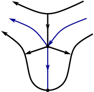
(a) $v=b$

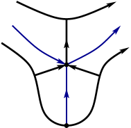
(b) $v=b^{-1}$

Figure 4. Schematic representation of the set $F$ (thiner arcs), arcs $\Gamma_{v}$, $\Gamma_{v,-1}$ (labeled), and $\Gamma_{v,1}$ (not labeled, placed symmetrically across $\Gamma_{v,-1}$), and the domains $\Omega_{\infty,1}$, $\Omega_{0,1}$, $\Omega_{v,1}$ (labeled) and $\Omega_{\infty,-1}$, $\Omega_{0,-1}$, $\Omega_{v,-1}$ (not labeled, placed symmetrically across the labeled ones) locally around $v\in\{b,b^{-1}\}$. The symbols $\oplus$ and $\ominus$ indicated whether the corresponding domain is a part of $\Omega_{+}$ or $\Omega_{-}$.

Moreover, we also introduce open oriented arcs $\Gamma_{v,1},\Gamma_{v,-1},\Gamma_{v}$ connecting $v$ to $\Gamma_{0}\cup\Gamma_{\infty}$, $v\in\big{\{}b,b^{-1}\big{\}}$, as shown on Figure 4. Besides the interior domain of $\Gamma_{0}$ and the exterior domain of $\Gamma_{\infty}$, the union of the introduced arcs, say $\Gamma$, together with $F$ delimits eight domains that we label as on Figure 4. Observe that $\rho$ has holomorphic and non-vanishing extension to each of these eight domains (we can bring arcs $\Gamma_{0},\Gamma_{\infty}$ closer to $F$ if necessary). We assume that all the introduced arcs are smooth. Define

(75) $$\boldsymbol{X}(z):=\boldsymbol{Y}(z)\left\{\begin{array}[]{rl}\left(\begin{matrix}1&0\\ \pm z^{n}/\rho(z)&1\end{matrix}\right),&z\in\Omega_{\pm},\vskip 6.0pt plus 2.0pt minus 2.0pt\\ \boldsymbol{I},&\text{otherwise}.\end{array}\right.$$

where $\Omega_{+}:=\Omega_{\infty,1}\cup\Omega_{\infty,-1}\cup\Omega_{b,-1}\cup\Omega_{b^{-1},1}$ and $\Omega_{-}:=\Omega_{0,1}\cup\Omega_{0,-1}\cup\Omega_{b,1}\cup\Omega_{b^{-1},-1}$. Then the Riemann-Hilbert problem for $\boldsymbol{X}$ can be formulated as follows:

• $\boldsymbol{X}$ is analytic in $\mathbb{C}\setminus(F\cup\Gamma)$ and $\displaystyle\lim_{z\to\infty}{\boldsymbol{X}}(z)z^{-n\sigma_{3}}=\boldsymbol{I}$;

• $\boldsymbol{X}$ has continuous traces at the smooth points of $F\cup\Gamma$ that satisfy

  $$\boldsymbol{X}_{+}(s)=\boldsymbol{X}_{-}(s)\left(\begin{matrix}0&\rho(s)/s^{n}\\ -s^{n}/\rho(s)&0\end{matrix}\right),$$

  for $s\in F^{\circ}$, as well as

  $$\boldsymbol{X}_{+}(s)=\boldsymbol{X}_{-}(s)\left(\begin{matrix}1&0\\ \pm s^{n}/\rho(s)&1\end{matrix}\right),$$

  for $s\in\big{(}\Gamma_{0}\cup\Gamma_{\infty}\big{)}\setminus\big{\{}a,a^{-1}\big{\}}$, where we need to use the sign $-$ for the portion of $\Gamma_{0}$ bordering $\Omega_{b,-1}$ and the part of $\Gamma_{\infty}$ bordering $\Omega_{b^{-1},-1}$, and

  $$\boldsymbol{X}_{+}(s)=\boldsymbol{X}_{-}(s)\left(\begin{matrix}1&0\vskip 6.0pt plus 2.0pt minus 2.0pt\\ s^{n}R(s)&1\end{matrix}\right),$$

  for $s\in\cup_{v\in\{b,b^{-1}\}}\big{(}\Gamma_{v}\cup\Gamma_{v,1}\cup\Gamma_{v,-1}\big{)}$, where we put $\rho_{e}:=\rho_{|F_{e}}$ for $e\in\big{\{}a,a^{-1},1,-1\big{\}}$ and set

  $$R(s):=\left\{\begin{array}[]{ll}-\rho_{a^{\pm 1}}(s)/(\rho_{1}\rho_{-1})(s),&s\in\Gamma_{b^{\pm 1}},\vskip 3.0pt plus 1.0pt minus 1.0pt\\ \rho_{1}(s)/(\rho_{-1}\rho_{a^{\pm 1}})(s),&s\in\Gamma_{b^{\pm 1},-1},\vskip 3.0pt plus 1.0pt minus 1.0pt\\ \rho_{-1}(s)/(\rho_{a^{\pm 1}}\rho_{1})(s),&s\in\Gamma_{b^{\pm 1},1};\end{array}\right.$$

• $\boldsymbol{X}$ satisfies RHP-${\boldsymbol{Y}}$(c) except around $a$ within $\Omega_{b,1}\cup\Omega_{b,-1}$ where it behaves like (67).

With the above changes, Lemma 12 holds with (57) replaced by (75).

7.2. Model and Local RH Problems

Model Riemann-Hilbert problem RHP-${\boldsymbol{N}}$ is formulated and solved exactly as in the case $\rho\in\mathcal{W}_{2}$ for $n\in\mathbb{N}_{\varepsilon}$.

Let now $U_{e}$ be an open set around $e\in E$. In the case of $U_{b^{\pm 1}}$ we shall further assume that these sets do not intersect $\Gamma_{0}\cup\Gamma_{\infty}$ and completely contain $\Gamma_{b^{\pm 1}},\Gamma_{b^{\pm 1},1},\Gamma_{b^{\pm 1},-1}$, see Figure 5.

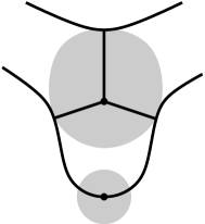
Figure 5. Schematic representation of the open sets $U_{e}$ for $e\in E$.

Define $\boldsymbol{D}(z):=\Phi(\boldsymbol{z})^{n\sigma_{3}}$, $\boldsymbol{z}\in D_{\mathcal{Q}}$, where $\Phi$ is given by (35) and the open set $D_{\mathcal{Q}}$ was defined just before Theorem 5. As in Section 6.3 we shall need to solve RHP-$\boldsymbol{P}_{e}$ for all $e\in E$. As in the previous proof, we postpone the construction of these matrix-functions until the end of the section.

7.3. RH Problem with Small Jumps

Let

$$\Sigma=\bigcup_{e\in E}\partial U_{e}\cup\left[\big{(}\Gamma_{0}\cup\Gamma_{\infty})\setminus\bigcup_{e\in E}\overline{U}_{e}\right].$$

The Riemann-Hilbert problem RHP-${\boldsymbol{Z}}$ now needs to be formulated as follows:

• $\boldsymbol{Z}$ is a holomorphic matrix function in $\overline{\mathbb{C}}\setminus\Sigma$ and $\boldsymbol{Z}(\infty)=\boldsymbol{I}$;

• $\boldsymbol{Z}$ has continuous traces on $\big{(}\Gamma_{0}\cup\Gamma_{\infty}\big{)}\setminus\bigcup_{e\in E}\overline{U}_{e}$ that satisfy

  $$\boldsymbol{Z}_{+}(s)=\boldsymbol{Z}_{-}(s)\boldsymbol{M}(s)\left(\begin{matrix}1&0\\ \pm s^{n}/\rho(s)&1\end{matrix}\right)\boldsymbol{M}^{-1}(s),$$

  where the choice of the sign $\pm$ is the same as in the second relation in RHP-${\boldsymbol{X}}$(b); and

  $$\boldsymbol{Z}_{+}(s)=\boldsymbol{Z}_{-}(s)\big{(}\boldsymbol{P}_{e}\boldsymbol{M}^{-1}\big{)}(s)$$

  on $\partial U_{e}$ for each $e\in E$.

Then the following lemma takes place.

Lemma 15.

For $n\in\mathbb{N}_{\varepsilon}$ large enough, a solution of RHP-${\boldsymbol{Z}}$ exists and satisfies $\boldsymbol{Z}=\boldsymbol{I}+\mathcal{O}\big{(}1/n\big{)}$ where $\mathcal{O}(\cdot)$ holds uniformly in $\overline{\mathbb{C}}$ and depends on $\varepsilon$.

Proof.

The proof of the fact that the jump of $\boldsymbol{Z}$ is geometrically small on $\big{(}\Gamma_{0}\cup\Gamma_{\infty}\big{)}\setminus\bigcup_{e\in E}\overline{U}_{e}$ is the same as in the case $\rho\in\mathcal{W}_{2}$. Furthermore, we have that

$$\boldsymbol{P}_{e}\boldsymbol{M}^{-1}=\boldsymbol{I}+\boldsymbol{MD}^{-1}\mathcal{O}(1/n)\boldsymbol{DM}^{-1}$$

on $\partial U_{e}$. It follows from (26), (27), (48), and the equality $\Phi(\boldsymbol{z})\Phi(\boldsymbol{z}^{*})=z$, see Lemma 6, that the first row of $\boldsymbol{MD}^{-1}$ is equal to

$$\left(\begin{matrix}(A_{n\tau+m_{n}}S_{h}\Theta_{n})(\boldsymbol{z})&\pm(A_{n\tau+m_{n}}S_{h}\Theta_{n})(\boldsymbol{z}^{*})\end{matrix}\right),\quad\boldsymbol{z}\in D_{\mathcal{Q}}.$$

It was shown in the course of the proof of Theorem 5 that these functions have uniformly bounded above moduli on compact subsets of $\mathbb{C}$. Similarly, one can show that the same is true for the second row of $\boldsymbol{MD}^{-1}$ as well. Since

$$\det\big{(}\boldsymbol{MD}^{-1}\big{)}=\det(\boldsymbol{M})=\big{(}\gamma_{n}\gamma_{n-1}^{\star}\big{)}^{-1},$$

and the constants $|\gamma_{n}\gamma_{n-1}^{\star}|$ are uniformly bounded above for all $n\in\mathbb{N}_{\varepsilon}$, we get that the jump of $\boldsymbol{Z}$ is of order $\boldsymbol{I}+\mathcal{O}(1/n)$ on $\partial U_{e}$ for each $e\in E$. The conclusion of the lemma now follows as in the case $\rho\in\mathcal{W}_{2}$. ∎

7.4. Asymptotics

Formulae (28) follow now exactly as in the case $\rho\in\mathcal{W}_{2}$.

7.5. Solution of RHP-$\boldsymbol{P}_{e}$ for $e\in\big{\{}a,a^{-1}\big{\}}$

As in Section 6.6, we shall only construct the matrix $\boldsymbol{P}_{a}$. The construction is still based on the matrix function $\boldsymbol{\Psi}_{\alpha}$ solving RHP-${\boldsymbol{\Psi}_{\alpha}}$. Again, we start by defining a special conformal map around $a$.

7.5.1. Conformal Map

With the notation used in Section 3.1, define

(76) $$\zeta_{a}(z):=\left(-\int_{a}^{z}\frac{v(s)}{4s}\mathrm{d}s\right)^{2},\quad z\in U_{a}.$$

Since $v_{+}=-v_{-}$ on $F_{a}^{\circ}$, $\zeta_{a}$ is holomorphic in $U_{a}$. Moreover, since $v$ has a square-root singularity at $a$, $\zeta_{a}$ has a simple zero at $a$. Thus, we can choose $U_{a}$ small enough so that $\zeta_{a}$ is conformal in $\overline{U}_{a}$. Recall that $v(s)\mathrm{d}s/s$ is purely imaginary on $F_{a}^{\circ}$, see the last part of the proof of Lemma 6. Therefore, $\zeta_{a}$ maps $F_{a}$ into the negative reals. As we have had some freedom in choosing the curve $\Gamma_{0}$, we shall choose it within $U_{a}$ so that the part of $\Gamma_{0}$ bordering $\Omega_{b,1}$, say $\Gamma_{0}^{+}$, is mapped into $I_{+}$ and the part bordering $\Omega_{b,-1}$, say $\Gamma_{0}^{-}$, is mapped into $I_{-}$. Notice that the orientation of $\zeta_{a}(\Gamma_{0}^{-})$ is the opposite from the one of $I_{-}$.

In what follows, we understand under $\zeta_{a}^{1/2}$ the branch given by the expression in parenthesis in (76). Equations (33) and (35) yield that

$$\zeta_{a}(z)=\left(\frac{1}{4}\log\left(\Phi\big{(}z^{(0)}\big{)}/\Phi\big{(}z^{(1)}\big{)}\right)\right)^{2},\quad z\in U_{a}.$$

As $\Phi(\boldsymbol{z})\Phi(\boldsymbol{z}^{*})\equiv z$, relation (72) remains valid for $\zeta_{a}$ as above and $\boldsymbol{D}(z)=\Phi(\boldsymbol{z})^{n\sigma_{3}}$, $\boldsymbol{z}\in D_{\mathcal{Q}}$. Finally, as in the case of real $a$, it still holds that $\zeta_{a+}^{1/4}=\mathrm{i}\zeta_{a-}^{1/4}$ on $F_{a}$.

7.5.2. Matrix $\boldsymbol{P}_{a}$

Let $J_{a}$ be the arc in $U_{a}$ emanating from $a$ such that $\zeta_{a}(J_{a})\subset[0,\infty)$. According to the conditions placed on the class $\mathcal{W}_{1}$, it holds that

$$\rho(z)=\rho_{*}(z)(z-a)^{\alpha},$$

where $\rho_{*}$ is non-vanishing and holomorphic in $U_{a}$ and $(z-a)^{\alpha}$ is the branch holomorphic in $U_{a}\setminus J_{a}$. Set $U_{a}^{\pm}$ to be connected components of $U_{a}\setminus(F_{a}\cup J_{a})$ containing $\Gamma_{0}^{\pm}$. Define

$$r_{a}(z):=\sqrt{\rho_{*}(z)}(a-z)^{\alpha/2},$$

where the branch $(a-z)^{\alpha/2}$ is holomorphic in $U_{a}\setminus F_{a}$ and chosen so

$$(a-z)^{\alpha}=e^{\pm\pi\mathrm{i}\alpha}(z-a)^{\alpha},\quad z\in U_{a}^{\pm}.$$

Then $r_{a}$ is a holomorphic and non-vanishing function in $U_{a}\setminus F_{a}$ and satisfies

$$\left\{\begin{array}[]{ll}r_{a+}(s)r_{a-}(s)=\rho(s),&s\in F_{a}\cap U_{a},\vskip 6.0pt plus 2.0pt minus 2.0pt\\ r_{a}^{2}(z)=\rho(z)e^{\pm\pi\mathrm{i}\alpha},&z\in\Gamma_{0}^{\pm}.\end{array}\right.$$

It can be readily verified now that a solution of RHP-$\boldsymbol{P}_{e}$ for $e=a$ is given by (73), (74).

7.6. Solution of RHP-$\boldsymbol{P}_{e}$ for $e\in\big{\{}b,b^{-1}\big{\}}$

We shall construct $\boldsymbol{P}_{b^{-1}}$ only as the construction of $\boldsymbol{P}_{b}$ is almost identical.

7.6.1. Model Problem

Recall (69). Let $\boldsymbol{\Psi}$ be a matrix-valued function such that

• $\boldsymbol{\Psi}$ is holomorphic in $\mathbb{C}\setminus\big{(}I_{+}\cup I_{-}\cup(-\infty,\infty)\big{)}$;

• $\boldsymbol{\Psi}$ has continuous traces on $I_{+}\cup I_{-}\cup(-\infty,0)\cup(0,\infty)$ that satisfy

  $$\boldsymbol{\Psi}_{+}=\boldsymbol{\Psi}_{-}\left\{\begin{array}[]{rll}\left(\begin{matrix}0&1\\ -1&0\end{matrix}\right)&\text{on}&(-\infty,0),\vskip 6.0pt plus 2.0pt minus 2.0pt\\ \left(\begin{matrix}1&0\\ 1&1\end{matrix}\right)&\text{on}&I_{\pm},\vskip 6.0pt plus 2.0pt minus 2.0pt\\ \left(\begin{matrix}1&1\\ 0&1\end{matrix}\right)&\text{on}&(0,\infty);\end{array}\right.$$

• $\boldsymbol{\Psi}(\zeta)=\mathcal{O}(1)$ as $\zeta\to 0$;

• $\boldsymbol{\Psi}$ has the following behavior near $\infty$:

  $$\boldsymbol{\Psi}(\zeta)=\boldsymbol{S}(\zeta)\left(\boldsymbol{I}+\mathcal{O}\left(\zeta^{-3/2}\right)\right)\exp\left\{-\frac{2}{3}\zeta^{3/2}\sigma_{3}\right\}$$

  uniformly in $\mathbb{C}\setminus\big{(}I_{+}\cup I_{-}\cup(-\infty,\infty)\big{)}$, where $\boldsymbol{S}(\zeta)$ was defined in RHP-${\boldsymbol{\Psi}_{\alpha}}$(d).

Such a matrix function was constructed in [8] with the help of Airy functions.

7.6.2. Conformal Map

With the notation used in Section 3.1, define

(77) $$\zeta_{b^{-1}}(z):=\left(-\frac{3}{4}\int_{b^{-1}}^{z}\frac{v(s)}{s}\mathrm{d}s\right)^{2/3},\quad z\in U_{b^{-1}}.$$

Because $v_{+}=-v_{-}$ on $F_{a^{-1}}^{\circ}$, $\zeta_{b^{-1}}^{3}$ is holomorphic in $U_{b^{-1}}$. Moreover, since $v$ vanishes as a square root when $z\to b^{-1}$, $\zeta_{b^{-1}}^{3}$ has a cubic zero at $b^{-1}$ and therefore $\zeta_{b^{-1}}$ is holomorphic in $U_{b^{-1}}$. The size of $U_{b^{-1}}$ can be adjusted so that $\zeta_{b^{-1}}$ is conformal in $U_{b^{-1}}$. Recall that the integral of $v(s)\mathrm{d}s/s$ is purely imaginary on $F$. Hence, we can select such a branch in (77) that

$$\zeta_{b^{-1}}(F_{a^{-1}}\cap U_{b^{-1}})\subset(-\infty,0].$$

Moreover, we always can adjust the system of arcs $\Gamma$ so that

$$\zeta_{b^{-1}}(\Gamma_{b^{-1},-1})\subset I_{+},\quad\zeta_{b^{-1}}(\Gamma_{b^{-1},1})\subset I_{-},\quad\text{and}\quad\zeta_{b^{-1}}(\Gamma_{b^{-1}})\subset(0,\infty).$$

In what follows, we understand under $\zeta_{b^{-1}}^{3/2}$ the branch given by the expression in parenthesis in (77) and select the branch of $\zeta_{b^{-1}}^{1/4}$ with the cut along $F_{a^{-1}}$ satisfying $\zeta_{b^{-1}+}^{1/4}=\mathrm{i}\zeta_{b^{-1}-}^{1/4}$.

Let $z\in U_{b^{-1}}\setminus(F_{a^{-1}}\cup F_{1})$ belong to the component containing $F_{-1}$, say $U_{b^{-1}}^{1}$, see Figures 4 and 5. Let $\gamma$ be a path from $a$ to $b^{-1}$ and $\gamma_{z}$ be a path from $b^{-1}$ to $z$ that lie entirely in $U_{b^{-1}}^{1}$. As usual denote by $B^{(i)}$ the lift of the set $B$ to $\boldsymbol{\mathfrak{S}}^{(i)}$. Then

(78) $$\gamma^{(0)}\cup\gamma_{z}^{(0)}\quad\text{and}\quad\gamma^{(0)}\cup\boldsymbol{\alpha}\cup\boldsymbol{\beta}\cup\gamma_{z}^{(1)}$$

are paths from $\boldsymbol{a}$ to $z^{(0)}$ and $z^{(1)}$, respectively, that belong to $\boldsymbol{\mathfrak{S}}_{\boldsymbol{\alpha},\boldsymbol{\beta}}$ (technically, $\boldsymbol{\alpha},\boldsymbol{\beta}$ in (78) need to be deformed into homologous cycles that belong to $\boldsymbol{\mathfrak{S}}_{\boldsymbol{\alpha},\boldsymbol{\beta}}$). Then by using (78) in (35) and recalling (34), we get that

$$\Phi\big{(}z^{(0)}\big{)}/\Phi\big{(}z^{(1)}\big{)}=\exp\left\{2\pi\mathrm{i}(\omega-\tau)+\frac{4}{3}\zeta_{b^{-1}}^{3/2}(z)\right\}.$$

Let now $z\in U_{b^{-1}}\setminus(F_{a^{-1}}\cup F_{1})$ be in the component that does not contain $F_{-1}$, say $U_{b^{-1}}^{2}$. Choose $\gamma_{z}$ to be a part of this component. Then

(79) $$\gamma^{(0)}\cup\gamma_{z}^{(0)}\quad\text{and}\quad\gamma^{(0)}\cup\boldsymbol{\alpha}\cup-\boldsymbol{\beta}\cup\gamma_{z}^{(1)}$$

are paths from $\boldsymbol{a}$ to $z^{(0)}$ and $z^{(1)}$, respectively, that belong to $\boldsymbol{\mathfrak{S}}_{\boldsymbol{\alpha},\boldsymbol{\beta}}$ (with the same caveat as before). Thus, we get from (79), (35), and (34) that

$$\Phi\big{(}z^{(0)}\big{)}/\Phi\big{(}z^{(1)}\big{)}=\exp\left\{-2\pi\mathrm{i}(\omega+\tau)+\frac{4}{3}\zeta_{b^{-1}}^{3/2}(z)\right\}.$$

Altogether, we get that

(80) $$\exp\left\{-\frac{2}{3}n\zeta_{b^{-1}}^{3/2}(z)\right\}=\big{(}\boldsymbol{KJD}\big{)}(z)z^{-n\sigma_{3}/2}\boldsymbol{J}^{-1}(z),$$

where

$$\boldsymbol{J}(z)=\left\{\begin{array}[]{rl}\left(\begin{matrix}0&1\\ -1&0\end{matrix}\right),&z\in D_{0}\cap U_{b^{-1}},\vskip 6.0pt plus 2.0pt minus 2.0pt\\ \boldsymbol{I},&\text{otherwise},\end{array}\right.$$

and

$$\boldsymbol{K}(z):=\left\{\begin{array}[]{rl}e^{\pi\mathrm{i}(\omega-\tau)n\sigma_{3}},&z\in U_{b^{-1}}^{1},\vskip 6.0pt plus 2.0pt minus 2.0pt\\ e^{-\pi\mathrm{i}(\omega+\tau)n\sigma_{3}},&z\in U_{b^{-1}}^{2}.\end{array}\right.$$

7.6.3. Matrix $\boldsymbol{P}_{b^{-1}}$

Set

$$r_{b^{-1}}(z):=\left\{\begin{array}[]{ll}\sqrt{(\rho_{1}\rho_{a^{-1}})(z)/\rho_{-1}(z)},&z\in U_{b^{-1}}^{2},\vskip 6.0pt plus 2.0pt minus 2.0pt\\ \sqrt{(\rho_{1}\rho_{-1})(z)/\rho_{a^{-1}}(z)},&z\in D_{0}\cap U_{b^{-1}}^{1},\vskip 6.0pt plus 2.0pt minus 2.0pt\\ \sqrt{(\rho_{a^{-1}}\rho_{-1})(z)/\rho_{1}(z)},&z\in D_{\infty}\cap U_{b^{-1}}^{1}.\end{array}\right.$$

Then it follows from RHP-${\boldsymbol{\Psi}}$(a,b,c) that

$$\boldsymbol{P}_{b^{-1}}(z):=\boldsymbol{E}_{b^{-1}}(z)\boldsymbol{\Psi}\big{(}n^{2/3}\zeta_{b^{-1}}(z)\big{)}\boldsymbol{J}(z)z^{n\sigma_{3}/2}r_{b^{-1}}^{-\sigma_{3}}(z)$$

satisfies RHP-$\boldsymbol{P}_{e}$(a,b,c) for $e=b^{-1}$, where $\boldsymbol{E}_{b^{-1}}$ is a holomorphic matrix in $U_{b^{-1}}$. Thus, it only remains to choose $\boldsymbol{E}_{b^{-1}}$ so that RHP-$\boldsymbol{P}_{e}$(d) is fulfilled. Set

$$\boldsymbol{E}_{b^{-1}}(z):=\boldsymbol{M}(z)\boldsymbol{D}^{-1}(z)r_{b^{-1}}^{\sigma_{3}}(z)\boldsymbol{J}^{-1}(z)\boldsymbol{K}^{-1}(z)\boldsymbol{S}^{-1}\big{(}n^{2/3}\zeta_{b^{-1}}(z)\big{)}.$$

Recall that $\boldsymbol{D}(z)=\Phi^{n\sigma_{3}}(\boldsymbol{z})$ for $\boldsymbol{z}\in D_{\mathcal{Q}}$. Denote the $(1,1)$-entry of $\boldsymbol{D}(z)$ by $d(z)$. Then

(81) $$(d_{-}d_{+})(s)=\left\{\begin{array}[]{rl}\Phi^{n}\big{(}s^{(1)}\big{)}\Phi^{n}\big{(}s^{(0)}\big{)},&s\in F_{-1},\vskip 6.0pt plus 2.0pt minus 2.0pt\\ \Phi_{+}^{n}\big{(}s^{(1)}\big{)}\Phi_{+}^{n}\big{(}s^{(0)}\big{)},&s\in F_{1},\vskip 6.0pt plus 2.0pt minus 2.0pt\\ \Phi_{+}^{n}\big{(}\boldsymbol{s}\big{)}\Phi_{+}^{n}\big{(}\boldsymbol{s}^{*}\big{)},&s\in F_{a^{-1}},\end{array}\right.=s^{n}\left\{\begin{array}[]{rl}1,&s\in F_{-1},\vskip 6.0pt plus 2.0pt minus 2.0pt\\ e^{2\pi\mathrm{i}\omega n},&s\in F_{1},\vskip 6.0pt plus 2.0pt minus 2.0pt\\ e^{2\pi\mathrm{i}\tau n},&s\in F_{a^{-1}},\end{array}\right.$$

by the property $\Phi(\boldsymbol{z})\Phi(\boldsymbol{z}^{*})=z$ and (36), where the traces of $d(z)$ are taken on the arcs in the complex plane and the traces of $\Phi(\boldsymbol{z})$ are taken on the cycles on $\boldsymbol{\mathfrak{S}}$. Using RHP-${\boldsymbol{N}}$(b), (70), (81), and the explicit definitions of $r_{b^{-1}}$, $\boldsymbol{J}$, and $\boldsymbol{K}$, it is tedious but straightforward to check that $\boldsymbol{E}_{b^{-1}}$ is holomorphic in $U_{b^{-1}}\setminus\big{\{}b^{-1}\big{\}}$. It also follows from (24) and the behavior of $\boldsymbol{S}$ at zero that

$$\boldsymbol{E}_{b^{-1}}(z)=\left(\begin{matrix}1&|z-b^{-1}|^{-1/2}\vskip 6.0pt plus 2.0pt minus 2.0pt\\ 1&|z-b^{-1}|^{-1/2}\end{matrix}\right)$$

which yields that it is, in fact, holomorphic on the whole set $U_{b^{-1}}$. The relation RHP-$\boldsymbol{P}_{e}$(d) now follows from RHP-${\boldsymbol{\Psi}}$(d) and (80).

References

• [1] A.I. Aptekarev and M. Yattselev. Padé approximants for functions with branch points — strong asymptotics of Nuttall-Stahl polynomials. Acta Math., 215(2):217–280, 2015. http://dx.doi.org/10.1007/s11511-016-0133-5.
• [2] L. Baratchart, H. Stahl, and M. Yattselev. Weighted extremal domains and best rational approximation. Adv. Math., 229:357–407, 2012. https://doi.org/10.1016/j.aim.2011.09.005.
• [3] L. Baratchart and M. Yattselev. Convergent interpolation to Cauchy integrals over analytic arcs. Found. Comput. Math., 9(6):675–715, 2009. https://doi.org/10.1007/s10208-009-9042-8.
• [4] L. Baratchart and M. Yattselev. Convergent interpolation to Cauchy integrals over analytic arcs with Jacobi-type weights. Int. Math. Res. Not., 2010(22):4211–4275, 2010. https://doi.org/10.1093/imrn/rnq026.
• [5] V.I. Buslaev. Convergence of multipoint Padé approximants of piecewise analytic functions. Sb. Math., 204(2):190–222, 2013.
• [6] V.I. Buslaev. Convergence of $m$-point Padé approximants of a tuple of multivalued analytic functions. Mat. Sb., 206(2):175–200, 2015.
• [7] P. Deift. Orthogonal Polynomials and Random Matrices: a Riemann-Hilbert Approach, volume 3 of Courant Lectures in Mathematics. Amer. Math. Soc., Providence, RI, 2000.
• [8] P. Deift, T. Kriecherbauer, K.T.-R. McLaughlin, S. Venakides, and X. Zhou. Strong asymptotics for polynomials orthogonal with respect to varying exponential weights. Comm. Pure Appl. Math., 52(12):1491–1552, 1999.
• [9] P. Deift and X. Zhou. A steepest descent method for oscillatory Riemann-Hilbert problems. Asymptotics for the mKdV equation. Ann. of Math., 137:295–370, 1993.
• [10] A.S. Fokas, A.R. Its, and A.V. Kitaev. Discrete Panlevé equations and their appearance in quantum gravity. Comm. Math. Phys., 142(2):313–344, 1991.
• [11] A.S. Fokas, A.R. Its, and A.V. Kitaev. The isomonodromy approach to matrix models in 2D quantum gravitation. Comm. Math. Phys., 147(2):395–430, 1992.
• [12] F.D. Gakhov. Boundary Value Problems. Dover Publications, Inc., New York, 1990.
• [13] A.A. Gonchar and E.A. Rakhmanov. Equilibrium distributions and the degree of rational approximation of analytic functions. Mat. Sb., 134(176)(3):306–352, 1987. English transl. in Math. USSR Sbornik 62(2):305–348, 1989.
• [14] A.B. Kuijlaars, K.T.-R. McLaughlin, W. Van Assche, and M. Vanlessen. The Riemann-Hilbert approach to strong asymptotics for orthogonal polynomials on $[-1,1]$. Adv. Math., 188(2):337–398, 2004.
• [15] G. López Lagomasino. Szegő theorem for polynomials orthogonal with respect to varying measures. In M. Alfaro et al., editor, Orthogonal Polynomials and their Applications, volume 1329 of Lecture Notes in Mathematics, pages 255–260, Springer, Berlin, 1988.
• [16] E.A. Rakhmanov. Orthogonal polynomials and S-curves. In J. Arvesú and G. López Lagomasino, editors, Recent Advances in Orthogonal Polynomials, Special Functions, and Their Applications, volume 578 of Contemporary Mathematics, pages 195–239. Amer. Math. Soc., Providence, RI, 2012.
• [17] T. Ransford. Potential Theory in the Complex Plane, volume 28 of London Mathematical Society Student Texts. Cambridge University Press, Cambridge, 1995.
• [18] H. Stahl. Extremal domains associated with an analytic function. I, II. Complex Variables Theory Appl., 4:311–324, 325–338, 1985.
• [19] H. Stahl. Structure of extremal domains associated with an analytic function. Complex Variables Theory Appl., 4:339–356, 1985.
• [20] H. Stahl. Orthogonal polynomials with complex valued weight function. I, II. Constr. Approx., 2(3):225–240, 241–251, 1986.
• [21] H. Stahl. The convergence of Padé approximants to functions with branch points. J. Approx. Theory, 91:139–204, 1997.
• [22] H. Stahl. Strong asymptotics for orthogonal polynomials with varying weights. Acta Sci. Math. (Szeged), 65:717–762, 1999.
• [23] M. Yattselev. Symmetric contours and convergent interpolation. Accepted for publication in J. Approx. Theory. https://doi.org/10.1016/j.jat.2017.10.003.
• [24] E.I. Zverovich. Boundary value problems in the theory of analytic functions in Hölder classes on Riemann surfaces. Russian Math. Surveys, 26(1):117–192, 1971.