Computing leaky modes of optical fibers using a FEAST algorithm for polynomial eigenproblems

Abstract.

An efficient contour integral technique to approximate a cluster of nonlinear eigenvalues of a polynomial eigenproblem, circumventing certain large inversions from a linearization, is presented. It is applied to the nonlinear eigenproblem that arises from a frequency-dependent perfectly matched layer. This approach is shown to result in an accurate method for computing leaky modes of optical fibers. Extensive computations on an antiresonant fiber with a complex transverse microstructure are reported. This structure is found to present substantial computational difficulties: Even when employing over one million degrees of freedom, the fiber model appears to remain in a preasymptotic regime where computed confinement loss values are likely to be off by orders of magnitude. Other difficulties in computing mode losses, together with practical techniques to overcome them, are detailed.

1. Introduction

In this paper, we bring together recent advances in contour integral eigensolvers and perfectly matched layers to improve techniques for computing transverse modes of optical fibers. Unlike classical step-index optical fibers, many emerging microstructured optical fibers do not have perfectly guided modes. Yet, they can quite effectively guide energy in leaky modes, also known as quasi-normal modes or resonances. Confinement losses of leaky modes, and their accurate computation, are of considerable practical importance. We approach this computation by solving a nonlinear (polynomial) eigenproblem obtained using a frequency-dependent perfectly matched layer (PML) and high order finite element discretizations.

The PML we use is the one recently studied by [21]. Although their essential idea is the same as the early works on PML [3, 4, 5], their work is better appreciated in the following context. While adapting the PML for source problems to eigenproblems, many [1, 12, 17] preferred a frequency-independent PML over a frequency-dependent PML. This is because for eigenproblems obtained using PML, the “frequency” is related to the unknown eigenvalue, so a frequency-dependent approach results in equations with a nonlinear dependence on the unknown eigenvalue, and hence a nonlinear eigenproblem. In contrast, a frequency-independent approach results in a standard linear generalized eigenproblem, for which many standard solvers exist. However, the authors of [21] made a compelling case for the use of frequency-dependent PML by showing an overall reduction in spurious modes and improved preasymptotic eigenvalue approximations. The price to pay in their approach is that instead of a linear eigenproblem, one must solve a nonlinear (rational) eigenproblem. Excluding a zero singularity, one can reduce this to a polynomial eigenproblem.

One of the goals of this paper is to show that such polynomial eigenproblems can be solved using a contour integral eigensolver, recently popularized in numerical linear algebra under the name “the FEAST algorithm” [13, 23]. Accordingly, we begin our study in Section 2 by introducing the algorithm and our adaptation of it to polynomial eigenproblems. We use a well-known linearization [9] of a degree $d$ polynomial eigenproblem to get a linear eigenproblem with $d$ times as many unknowns as the original nonlinear eigenproblem. This $d$-fold increase in size is prohibitive, especially for applications like the computation of leaky optical modes, which, as we shall see in Section 4, will need several millions of degrees of freedom (before linearization). In Section 2, we show how to overcome this problem. Exploiting the fact that FEAST only requires the application of the resolvent of the linearization, we develop an identity for this large linearized resolvent in terms of smaller nonlinear resolvents of the original size. This leads to our eigensolver presented in Algorithm 1.

In Section 3, we formulate the equations for the transverse leaky modes of general optical fibers nondimensionally, introduce the equations of frequency-dependent PML, use an arbitrary order finite element discretization, and present the resulting cubic eigenproblem. The algorithm developed in the previous section is then applied. An interesting feature that derives from the combination of this discretization with our algorithm is that any spurious mode formed of finite element functions supported only in the PML region is automatically eliminated from the output eigenspace. This is because the formulation sends such functions to the eigenspace of $\infty$. This section also has a verification of the correctness of our approach using a semianalytical calculation for leaky modes of step-index fibers.

(a) Shaded and white areas indicate glass and air, respectively

(b) Zoomed in view near the top capillary tube

Figure 1. Transverse geometry of a microstructured fiber [18, 22, 30]

In Section 4, we consider a microstructured optical fiber. Recent microstructured fibers fall into two categories: photonic band gap fibers, and antiresonant fibers. Emerging fibers of the latter class seem not to have received much attention in the mathematical literature, although they are actively pursued in the optics literature [18, 22, 30]. Antiresonant optical fiber designs with air-filled hollow cores are particularly interesting since dispersion, nonlinear optical effects, and propagation losses are all negligible in air. We study such a fiber in Section 4, providing enough detail in the hope that it may serve as a benchmark problem for others. The fiber geometry is illustrated in Figure 1.

Some of the difficulties we encountered while computing the mode losses in Section 4 are worth noting here. For microstructured fibers with thin structural elements, we have generally found it difficult to find perfect agreement between our converged loss values and those reported in the optics literature produced using proprietary software. Our results in Section 4 illuminate the issue. For the fiber we considered, we found a surprisingly large preasymptotic regime where confinement loss values jump orders of magnitude when mesh size ($h$) and finite element degree ($p$) are varied. Hence it seems possible to find agreement with whatever loss value in the literature, experimental or numerical, by simply adjusting model and PML parameters, while the discretization is in the preasymptotic regime. But such agreement is meaningless. In view of the results of Section 4, we cannot recommend trusting computed resonance values and confinement losses reported without any evidence of them having stabilized over variations in $h$ and $p$ (or unsupported by other convergence studies). We will show multiple routes to get to the asymptotic regime of converging eigenvalues by either decreasing $h$ or by increasing $p$. In our experience, quicker routes to this asymptotic regime are generally offered by the latter.

While searching for core modes in such microstructured fibers, one should be wary of modes that carry energy in structures outside of the hollow core. Although these are unwanted modes, they are not spurious modes—they are actual eigenmodes of the structure. (Figure 7 shows such unwanted non-core modes; cf. core modes in Figure 6.) Another issue, well-recognized by many [1, 12, 17, 21] in other resonance computations, is the interference of spurious modes that arise from the discretization of the essential spectrum (and Figure 3 in this paper also provides a glimpse of this issue). In Section 4, we indicate a way to overcome this problem to some extent by using an elliptical contour in our eigensolver. Considering the expected deformation of the essential spectrum due to the PML, one may adjust the eccentricity of the ellipse to probe spectral regions of interest fairly close to the origin without wasting computational resources on unwanted eigenfunctions from the deformed essential spectrum.

In Section 5, we present proofs of the two theorems presented in the next section. We close with concluding remarks in Section 6.

2. A FEAST algorithm for polynomial eigenproblems

Consider the problem of finding a targeted cluster of nonlinear eigenvalues, enclosed within a given contour, and its associated eigenspace. (The problem of interest is precisely stated as Problem 1 in Subsection 2.2 below.) The FEAST algorithm [13, 16, 23] is one type of contour integral eigensolver that addresses such problems. A version of the algorithm for nonlinear eigenproblems was presented in [8], but here we shall pursue specific simplifications possible when the nonlinearity is of polynomial type. We begin by describing the standard FEAST algorithm for linear eigenproblems. Consider $A,B\in\mathbb{C}^{n\times n}$ and the linear generalized eigenproblem of finding numbers $\lambda\in\mathbb{C},$ an associated (right) eigenvector $0\neq x\in\mathbb{C}^{n}$, and a left eigenvector $0\neq\tilde{x}\in\mathbb{C}^{n}$, satisfying

$$\tilde{x}^{*}A=\lambda\tilde{x}^{*}B,\qquad Ax=\lambda Bx.$$ (1)

We shall also consider left and right generalized eigenvectors of such eigenproblems, since they are needed to formulate an accurate relation between ranges of certain spectral projectors at the foundation of the algorithm. Recall that the left and right algebraic eigenspaces (or generalized eigenspaces) of a linear eigenvalue are, respectively, the spans of its left and right generalized eigenvectors. Generalizations of these concepts to the nonlinear case are defined in Subsection 2.2.

2.1. Spectral projector approximation

Suppose we want to compute a cluster of eigenvalues, collected into a set $\varLambda$, and its accompanying (right) algebraic eigenspace, denoted by $E\subset\mathbb{C}^{n}$, and left algebraic eigenspace $\tilde{E}\subset\mathbb{C}^{n}$. The wanted eigenvalues, namely elements of $\varLambda,$ are known to be enclosed within $\varGamma$, a positively oriented, bounded, simple, closed contour that does not cross any eigenvalue.

The matrix-valued integrals

$$S=\frac{1}{2\pi\hat{\imath}}\oint_{\varGamma}(zB-A)^{-1}B\,dz,\qquad\tilde{S}=\frac{1}{2\pi\hat{\imath}}\oint_{\varGamma}(zB-A)^{-*}B^{*}\,dz,$$ (2)

sometimes called Riesz projections, or spectral projectors, are well known to yield projections onto the eigenvalue cluster’s right and left algebraic eigenspaces $E$ and $\tilde{E}$, respectively (see e.g., [15, page 39] or [6, Theorem 1.5.4]). Here and throughout, we use ^∗ and ^′ to denote conjugate transpose and transpose, respectively, so $M^{*}=\bar{M}^{\prime}$ for any matrix $M$ and we abbreviate $(M^{*})^{-1}$ to $M^{-*}$ for invertible $M$. Focusing on $E$ for the moment, $E$ is the eigenspace of $S$ associated to its eigenvalue one. The only other eigenvalue of $S$ is zero. The algebraic eigenspaces of all the eigenvalues of (1) not enclosed by $\varGamma$ have been mapped to the eigenspace of the zero eigenvalue of $S$. Hence, if we can compute $S$, then a well-known generalization of the power iteration (namely the subspace iteration) when applied to $S$ will converge to $E$ in one iteration. Along the same lines, we also conclude that a subspace iteration with $\tilde{S}$ will converge at once to $\tilde{E}$.

The FEAST algorithm is simply a subspace iteration, performed after replacing $S$ and $\tilde{S}$ by computable quadrature approximations.These quadrature approximations of $S$ and $\tilde{S}$ take the form

$$S_{N}=\sum_{k=0}^{N-1}w_{k}(z_{k}B-A)^{-1}B,\qquad\tilde{S}_{N}=\sum_{k=0}^{N-1}\bar{w}_{k}(z_{k}B-A)^{-*}B^{*},$$ (3)

for some $w_{k}\in\mathbb{C}$ and points $z_{k}\in\varGamma$. Then, the mathematical statement of the FEAST algorithm is as follows: given initial right and left subspaces $E_{0},\tilde{E}_{0}\subset\mathbb{C}^{n}$, compute two sequences of subspaces, $E_{\ell}$ and $\tilde{E}_{\ell}$, by

$$E_{\ell}=S_{N}E_{\ell-1},\qquad\tilde{E}_{\ell}=\tilde{S}_{N}\tilde{E}_{\ell-1}\qquad\text{ for }\ell=1,2,\ldots.$$ (4)

Here and throughout we use $MZ$ to denote $\{Mz:z\in Z\}$ for a matrix $M\in\mathbb{C}^{n\times n}$ and a subspace $Z\subseteq\mathbb{C}^{n}$. A practical implementation of the FEAST algorithm is not as simple as (4) because it must additionally take care of normalization and computation of Ritz values for each subspace iterate [13, 16, 23].

In this paper, we will use only circular and elliptical contours for $\varGamma$. Both have been studied previously [10, 13], so we will be brief. Letting $\phi=\pi/N$, we parametrize a circle $\varGamma$ of radius $\gamma>0$ centered at $y\in\mathbb{C}$, in terms of $\theta$, by $\varGamma=\{\gamma\exp(\hat{\imath}(\theta+\phi)+y:0\leq\theta<2\pi\}$. Transforming the integrals over $z$ in (2) as integrals over $\theta$, and then applying the trapezoidal rule at equally spaced $N$ values of $\theta$, shifted by $\phi$, we obtain a quadrature approximation of $S$ as in (3), with

$$\theta_{k}=\frac{2\pi k}{N},\quad z_{k}=\gamma\exp(\hat{\imath}(\theta_{k}+\phi))+y,\quad w_{k}=\frac{\gamma}{N}\exp(\hat{\imath}(\theta_{k}+\phi).$$ (5)

By estimating the separation between wanted and unwanted eigenvalues after the spectral mapping by $S_{N}$, it is possible to estimate the rate of convergence of the subspace iteration (4) while employing this quadrature (see e.g., [10, Example 2.2] or [13]).

We will also use elliptical contours later. Letting $\gamma>0,\rho>1,y\in\mathbb{C}$, we restrict ourselves to Bernstein ellipses $\varGamma=\{y+\gamma e^{\hat{\imath}\theta}\rho/(\rho+\rho^{-1})+\gamma e^{-\hat{\imath}\theta}\rho^{-1}/(\rho+\rho^{-1}):0\leq\theta<2\pi\}$ aligned with the coordinate axes. We again use an $N$ point uniform trapezoidal rule, shifting the ellipse parametrization $\theta$ by $\phi=\pi/N$. Simple computations then lead to the formulas

$$z_{k}=y+\gamma\frac{\rho e^{\hat{\imath}(\theta_{k}+\phi)}+\rho^{-1}e^{-\hat{\imath}(\theta_{k}+\phi)}}{\rho+\rho^{-1}},\quad w_{k}=\gamma\frac{\rho e^{\hat{\imath}(\theta_{k}+\phi)}-\rho^{-1}e^{-\hat{\imath}(\theta_{k}+\phi)}}{N(\rho+\rho^{-1})}$$ (6)

where $\theta_{k}=2\pi k/N$. These are the values we shall use in (3) when we need elliptical contours later.

2.2. Polynomial eigenproblems

In this subsection we establish notation for polynomial eigenproblems and consider a nonlinear eigenvalue cluster approximation problem. Suppose we are given $d+1$ matrices $A_{i}\in\mathbb{C}^{n\times n}$, $i=0,\ldots,d$. We assume that the last matrix $A_{d}$ is nonzero (in order to fix the grade $d$), but do not assume that $A_{d}$ is invertible. Let $\mathbb{C}^{+}=\mathbb{C}\cup\{\infty\}$, the extended complex plane. We consider the polynomial eigenproblem of finding a $\lambda\in\mathbb{C}^{+}$ satisfying

$$P(\lambda)x=0,\quad\tilde{x}^{*}P(\lambda)=0$$ (7a)

for some nontrivial $$x,\tilde{x}\in\mathbb{C}^{n} P(z) d$$, called the nonlinear right and left eigenvectors, respectively. Here is a matrix polynomial of degree , given by

$$P(z)=\sum_{j=0}^{d}z^{j}A_{j}.$$ (7b)

Since $P(z)$ is a square matrix, $\lambda$ may equivalently be thought of as a root of the nonlinear equation $\det P(z)=0$. The algebraic multiplicity of the nonlinear eigenvalue $\lambda$ is its multiplicity as a root of the polynomial $\det P(z)$, a polynomial which we assume does not vanish everywhere. Note that $\lambda=\infty$ is said to be an eigenvalue of (7) if zero is an eigenvalue of $z^{d}P(z^{-1})=z^{d}A_{0}+z^{d-1}A_{1}+\cdots+A_{d}$ [14, 28].

Next, let $P^{(l)}(z)$ denote the $l^{\text{th}}$ derivative ($d^{l}P/dz^{l}$) of $P$ with respect to the complex variable $z$. Ordered sequences $x_{0},x_{1},\ldots,x_{k-1}$ and $\tilde{x}_{0},\tilde{x}_{1},\ldots,\tilde{x}_{k-1}$ in $\mathbb{C}^{n}$ are respectively called [14] right and left Jordan chains for the matrix polynomial $P$ at $\lambda$ if

$$\sum_{l=0}^{j}\frac{1}{l!}P^{(l)}(\lambda)x_{j-l}=0,\qquad\sum_{l=0}^{j}\frac{1}{l!}\tilde{x}_{j-l}^{*}P^{(l)}(\lambda)=0,\qquad j=0,1,\ldots,k-1.$$ (8)

When $k=1$, the chains reduce to singletons and (8) coincides with the equation for an eigenvector (7a). For more general $k$, the vectors of these chains are referred to as (right and left) nonlinear generalized eigenvectors. The right and left algebraic eigenspaces of a set of nonlinear eigenvalues $\varLambda$ are, respectively, the span of all the right and left nonlinear generalized eigenvectors associated to every $\lambda$ in $\varLambda$. These definitions generalize the standard notion of algebraic eigenspace for the linear eigenproblem: indeed, in basic linear algebra, one respectively calls the sequences $x_{0},x_{1},\ldots,x_{k-1}\in\mathbb{C}^{n}$ and $\tilde{x}_{0},\tilde{x}_{1},\ldots,\tilde{x}_{k-1}\in\mathbb{C}^{n}$ a right and left Jordan chain of $A-\lambda B\in\mathbb{C}^{n\times n}$ if, for all $i=1,2,\ldots,k-1,$

$$(A-\lambda B)x_{0}=0,\text{ and }(A-\lambda B)x_{i}=Bx_{i-1},$$ (9a)

$$\tilde{x}_{0}^{*}(A-\lambda B)=0,\text{ and }\tilde{x}_{i}^{*}(A-\lambda B)=\tilde{x}_{i-1}^{*}B.$$ (9b)

It is easy to see that (9a) and (9b) are respectively equivalent to the first and second equalities of (8), when $P(\lambda)$ is set to the linear matrix polynomial $A-\lambda B$. With these notions, we can state the nonlinear analogue of the eigenvalue cluster approximation problem considered in Section 2.1.

Problem 1.

Compute a cluster $\varLambda$ of nonlinear eigenvalues of $P(z)$ enclosed within $\varGamma$ and its accompanying right and left algebraic eigenspaces $E$ and $\tilde{E}$, respectively.

In the study of matrix polynomials, the concept of a linearization is crucial [9]. The first companion linearization of $P(z)$ is the matrix pencil $\mathcal{A}-z\mathcal{B}\in\mathbb{C}^{nd\times nd}$, shown below in a $d\times d$ block partitioning where the blocks are elements of $\mathbb{C}^{n\times n}$:

$$\mathcal{A}=\begin{bmatrix}0&I&0&\cdots&0\\ 0&0&I&\ddots&\vdots\\ \vdots&\vdots&\ddots&\ddots&0\\ 0&0&\cdots&0&I\\ A_{0}&A_{1}&\cdots&A_{d-2}&A_{d-1}\end{bmatrix},\quad\mathcal{B}=\begin{bmatrix}I&0&\cdots&\cdots&0\\ 0&I&\ddots&&\vdots\\ \vdots&\ddots&\ddots&\ddots&\vdots\\ \vdots&&\ddots&I&0\\ 0&\cdots&\cdots&0&-A_{d}\end{bmatrix}.$$ (10)

Here and throughout, $I$ denotes the identity matrix (whose dimensions may differ at different occurrences, but will always be clear from context). Let us note a well known connection between the nonlinear eigenproblem (7) and the linear eigenproblem

$$\mathcal{A}X=\lambda\mathcal{B}X,\qquad\tilde{X}^{*}\mathcal{A}=\lambda\tilde{X}^{*}\mathcal{B},$$ (11)

for nontrivial left and right eigenvectors $X$ and $\tilde{X}$, respectively, and a “linear” eigenvalue $\lambda$. We block partition $Y\in\mathbb{C}^{nd\times m}$ using blocks $Y_{i}$ in $\mathbb{C}^{n\times m}$ (where the $m=1$ case represents a block partitioning of column vectors) as shown below, where we also define $F\in\mathbb{C}^{n\times nd}$ and $L\in\mathbb{C}^{n\times nd},$ all using a block partitioning compatible with (10):

$$Y=\begin{bmatrix}Y_{0}\\ Y_{1}\\ \vdots\\ Y_{d-1}\end{bmatrix},\quad F=\begin{bmatrix}I&0&\cdots&0\end{bmatrix},\quad L=\begin{bmatrix}0&0&\cdots&I\end{bmatrix}.$$ (12)

It is well known [9] that $\lambda$ is a nonlinear eigenvalue of the polynomial eigenproblem (7) of algebraic multiplicity $k$ if and only if it is a linear eigenvalue of algebraic multiplicity $k$ of the linearization (11). Hence researchers [28] have pursued the computation of polynomial eigenvalues by standard eigensolvers applied to the linear eigenproblem (11). To do so using the FEAST algorithm, the connection between the eigenspaces of (11) and (7) must be made precise, as done in Theorem 2 below using $F$ and $L$. Let us first describe the ingredients of the algorithm applied to the linearization.

Replacing $A,B$ by $\mathcal{A},\mathcal{B},$ respectively, in (2) and (3) we define $\mathcal{S},\tilde{\mathcal{S}},\mathcal{S}_{N},$ and $\tilde{\mathcal{S}}_{N}$:

$$\mathcal{S} =\frac{1}{2\pi\hat{\imath}}\oint_{\varGamma}(z\mathcal{B}-\mathcal{A})^{-1}\mathcal{B}\,dz, \tilde{\mathcal{S}}=\frac{1}{2\pi\hat{\imath}}\oint_{\varGamma}(z\mathcal{B}-\mathcal{A})^{-*}\mathcal{B}^{*}\,dz,$$ (13)

$$\mathcal{S}_{N} =\sum_{k=0}^{N-1}w_{k}(z_{k}\mathcal{B}-\mathcal{A})^{-1}\mathcal{B}, \tilde{\mathcal{S}}_{N}=\sum_{k=0}^{N-1}\bar{w}_{k}(z_{k}\mathcal{B}-\mathcal{A})^{-*}\mathcal{B}^{*}.$$

Given initial right and left subspaces $\mathcal{E}_{0},\tilde{\mathcal{E}}_{0}\subset\mathbb{C}^{nd}$, the FEAST algorithm, as written out in (4), computes a sequence of subspaces $\mathcal{E}_{\ell},\tilde{\mathcal{E}}_{\ell}$ by

$$\mathcal{E}_{\ell}=\mathcal{S}_{N}\mathcal{E}_{\ell-1},\qquad\tilde{\mathcal{E}}_{\ell}=\tilde{\mathcal{S}}_{N}\tilde{\mathcal{E}}_{\ell-1}\qquad\text{ for }\ell=1,2,\ldots.$$ (14)

In analogy with $E$ and $\tilde{E}$, we denote the right and left algebraic eigenspaces of $z\mathcal{B}-\mathcal{A}$ associated to its (linear) eigenvalues enclosed within $\varGamma$ by $\mathcal{E}$ and $\tilde{\mathcal{E}}$, respectively. Of course, they are [15], respectively, the ranges of the Riesz projections $\mathcal{S}$ and $\tilde{\mathcal{S}}$. The relationships between these spaces and the algebraic eigenspaces of the nonlinear $P(z)$ are given in the next result, which can be concluded from well known results on matrix polynomials. We give a self-contained proof in Section 5.

Theorem 2.

Let $E$ and $\tilde{E}$ be the right and left algebraic eigenspaces of the nonlinear eigenvalues of $P(z)$ enclosed in $\varGamma$, respectively. Then

1. $E=F\mathcal{E}$,

2. $\tilde{E}=L\tilde{\mathcal{E}}$.

In view of Theorem 2, when the FEAST algorithm (14) converges to $\mathcal{E},\tilde{\mathcal{E}}$, mere truncation by $F$ and $L$ is guaranteed to yield the algebraic eigenspaces needed in Problem 1.

Remark 3.

FEAST algorithms employing other contour integrals that can provably recover the wanted spaces $E,\tilde{E}$ (like in Theorem 2) are worthy of pursuit. To indicate why this might not be trivial, consider

$$S_{1}=\frac{1}{2\pi\hat{\imath}}\oint_{\varGamma}P(z)^{-1}\,dz.$$

Even if it might appear to be a reasonable nonlinear generalization of the linear resolvent integral, for $P(z)=(z^{2}-1)A$ with any invertible $A\in\mathbb{C}^{n\times n}$, one can easily verify that $S_{1}=0$ when $\varGamma$ encloses both the nonlinear eigenvalues $\pm 1$ of $P(z)$. See also $S_{2}$ in Remark 5.

2.3. An algorithm for solving polynomial eigenproblems

In this subsection, we describe an efficient implementation of (14). Implementing (14) as stated would require the inversion of $N$ linear systems of size $nd\times nd$, significantly larger than the size of the $n\times n$ matrix polynomial $P(\lambda)$. For large $nd$, due to the fill-in of sparse factorizations, applying and storing $(z_{k}\mathcal{B}-\mathcal{A})^{-1}$ at each quadrature point $z_{k}$ becomes very expensive. This drawback is particularly serious for our application in Section 4, where as we shall see, each $A_{i}$ is given as a large sparse matrix with $n\approx 10^{7}$. Therefore, we propose an implementation requiring only the inversion (or sparse factorization) of $n\times n$ matrices (rather than $nd\times nd$ matrices) at each quadrature point $z_{k}$, using the next result.

Theorem 4.

Suppose $P(z)$ is invertible at some $z\in\mathbb{C}$ and consider $X,Y,W\in\mathbb{C}^{nd}$ block partitioned as in (12). Then the following identities hold.

1. The block components of $X=(z\mathcal{B}-\mathcal{A})^{-1}Y$ are given by

   $$X_{0} =P(z)^{-1}\left(-Y_{d-1}-A_{d}Y_{d-1}+\sum_{i=1}^{d}A_{i}\sum_{j=0}^{i-1}z^{i-1-j}Y_{j}\right)$$ (15a)

   $$X_{i} =zX_{i-1}-Y_{i-1},\qquad i=1,2,\ldots,d-1.$$ (15b)

2. The block components of $\tilde{X}=(z\mathcal{B}-\mathcal{A})^{-*}W$ are given by

   $${\tilde{X}}_{d-1} =-P(z)^{-*}\sum_{j=0}^{d-1}\bar{z}^{j}W_{j},\quad{\tilde{X}}_{d-2}=-W_{d-1}-\bar{z}A_{d}^{*}{\tilde{X}}_{d-1}-A_{d-1}^{*}{\tilde{X}}_{d-1},$$ (16a)

   $${\tilde{X}}_{i} =-W_{i+1}+\bar{z}{\tilde{X}}_{i+1}-A_{i+1}^{*}{\tilde{X}}_{d-1},\qquad i=0,1,\ldots,d-3.$$ (16b)

Algorithm 1 Polynomial FEAST Eigensolver for Problem 1

Input contour $\varGamma$, quadrature $z_{k},w_{k}$, sparse coefficient matrices $A_{0},\ldots,A_{d-1},A_{d}\in\mathbb{C}^{n\times n}$, initial right and left eigenvector iterates given as columns of $Y,\tilde{Y}\in\mathbb{C}^{nd\times m}$, respectively, block partitioned as in (12) into $Y_{j},\tilde{Y}_{j}\in\mathbb{C}^{n\times m}$, and tolerance $\varepsilon>0$.

[kw] setup
+ Prepare $P(z_{k})^{-1}$ by sparse factorization at each quadrature point $z_{k}$.
- repeat
+ Set all entries of workspace $\tilde{R},R\in\mathbb{C}^{nd\times m}$ to $0$.
for each $z_{k}$, $k=0,\ldots,N-1$, do:
+ Compute block components of $X\in\mathbb{C}^{nd\times m}$:
+ $\displaystyle{X_{0}\leftarrow P(z_{k})^{-1}\sum_{i=1}^{d}\sum_{j=0}^{i-1}z_{k}^{i-1-j}A_{i}Y_{j},}$
for $i=1,\ldots,d-1$ do:   $\displaystyle{X_{i}\leftarrow z_{k}X_{i-1}-Y_{i-1}}$.
- Increment $R\mathrel{+}=w_{k}X$.
Compute block components of $\tilde{X}\in\mathbb{C}^{nd\times m}$:
+ $\displaystyle{\tilde{X}_{d-1}\leftarrow P(z_{k})^{-*}\sum_{j=0}^{d-1}\bar{z}_{k}^{j}\tilde{Y}_{j},}$
$\displaystyle{\tilde{X}_{d-2}\leftarrow-\tilde{Y}_{d-1}-\bar{z}_{k}A_{d}^{*}\tilde{X}_{d-1}-A_{d-1}^{*}\tilde{X}_{d-1}},$
for $i=d-3,\ldots,1,0,$  do:   $\displaystyle{\tilde{X}_{i}\leftarrow A_{i+1}^{*}\tilde{X}_{d-1}-\tilde{Y}_{i+1}+\bar{z}_{k}\tilde{X}_{i+1}.}$  
- Increment $\tilde{R}\mathrel{+}=\bar{w}_{k}\tilde{X}$.
- endfor
$G\leftarrow\tilde{R}^{*}\mathcal{B}R$.
Compute biorthogonal $V,\tilde{V}\in\mathbb{C}^{m\times m}$ such that $\tilde{V}^{*}GV=\mathop{\mathrm{diag}}(d_{1},\ldots,d_{m}).$
$Y\leftarrow RV$,   $\tilde{Y}\leftarrow\tilde{R}\tilde{V}$.
for $\ell=1,\ldots,m$ do:
+ If $d_{\ell}\approx 0$: then remove $\ell$th columns of $\tilde{Y}$ and $Y$,
else: rescale $\ell$th column of $\tilde{Y}$ and $Y$ by $|d_{\ell}|^{-1/2}$.
- endfor
Assemble small Ritz system: $A_{Y}\leftarrow\tilde{Y}^{*}\mathcal{A}Y$,  $B_{Y}\leftarrow\tilde{Y}^{*}\mathcal{B}Y$.
Compute Ritz values $\varLambda=\mathop{\mathrm{diag}}(\lambda_{1},\ldots,\lambda_{m})$ and $W,\tilde{W}\in\mathbb{C}^{m\times m}$ satisfying
& $\tilde{W}^{*}A_{Y}W=\varLambda$,  $\tilde{W}^{*}B_{Y}W=I$.
$Y\leftarrow YW$,  $\tilde{Y}\leftarrow\tilde{Y}\tilde{W}$.
Periodically check: if $\lambda_{\ell}$ falls outside $\varGamma$, remove $\ell$th columns of $Y$ and $\tilde{Y}$.
- until maximal difference of successive $\varLambda$ iterates is less than $\varepsilon$.
output eigenvalue cluster $\{\lambda_{\ell}\}$, left & right eigenvectors in columns of $L\tilde{Y}$ and $FY$.

Theorem 4 is proved in Section 5. A FEAST implementation based on it is given in Algorithm 1, which we now describe. The algorithm is written with small $(m)$ eigenvalue clusters and large $(n)$ sparse $A_{i}$ in mind ($m\ll n$). We also have in mind semisimple eigenvalues, since we want to use standard software tools for small diagonalizations (avoiding the complex issue of stable computation of generalized eigenvectors). Computation of $\mathcal{S}_{N}Y$ and $\tilde{\mathcal{S}}_{N}\tilde{Y}$ occur in steps 1–1 and 1–1 of Algorithm 1, via the identities of Theorem 4. After the computation of $\mathcal{S}_{N}Y$ and $\tilde{\mathcal{S}}_{N}\tilde{Y}$, the algorithm assembles a small ($m\times m$) Ritz system, based on the new eigenspace iterate, in step 1. Subsequently, step 1 attempts to diagonalize this. In practice, one must also handle exceptions in the event this diagonalization fails due to a (close to) defective eigenvalue, details which we have omitted from Algorithm 1, since we did not need them in our application.

Recall that we do not require $\mathcal{B}$ to be invertible. Lines 1–1 of the algorithm remove vectors in $\mathcal{K}=\ker\mathcal{B}$, the null space of $\mathcal{B}$, from the iteration. It is immediate from (13) that $\mathcal{K}$ is contained in the eigenspaces of $\mathcal{S}$ and $\mathcal{S}_{N}$ associated to their zero eigenvalue. Since these operators have their dominant eigenvalue away from zero, the subspace iteration (14) will filter out elements of $\mathcal{K}$ from its iterates. Let $K=\ker A_{d}$. Note that $\mathcal{K}=L^{\prime}\,K$. From the definitions in Subsection 2.2, it is obvious that any nontrivial element of $K$ is an eigenvector of (7) corresponding to eigenvalue $\infty.$ Therefore, $\mathcal{K}$ being filtered out amounts to filtering out the eigenspace of $\lambda=\infty$.

In the optics applications we are about to consider in the next two sections, $A_{d}$ turns out to be Hermitian and negative semidefinite. Then, $\mathcal{B}=\mathcal{B}^{*}$ is positive semidefinite and $(x,y)_{\mathcal{B}}=y^{*}\mathcal{B}x$ defines a semi-inner product (and an inner product on $\mathcal{K}^{\perp}$). Moreover, it is easy to see that

$$(\mathcal{S}x,y)_{\mathcal{B}}=(x,\tilde{\mathcal{S}}y)_{\mathcal{B}},\qquad(\mathcal{S}_{N}x,y)_{\mathcal{B}}=(x,\tilde{\mathcal{S}}_{N}y)_{\mathcal{B}}$$ (17)

for all $x,y\in\mathbb{C}^{nd}$, i.e., $\tilde{\mathcal{S}}$ and $\tilde{\mathcal{S}}_{N}$ are the $\mathcal{B}$-adjoints of $\mathcal{S}$ and $\mathcal{S}_{N}$, respectively. The first equation of (17) implies that $(\mathcal{E},\ker\tilde{\mathcal{S}})_{\mathcal{B}}=0$. Hence the wanted right eigenfunctions (in $\mathcal{E}$) are $\mathcal{B}$-orthogonal to the unwanted left ones (in $\ker\tilde{\mathcal{S}}$), and vice versa, since we also have $(\ker\mathcal{S},\tilde{\mathcal{E}})_{\mathcal{B}}=0$. When the iterates $Y,\tilde{Y}$ of Algorithm 1 converge, their respective column spaces inherit these orthogonality properties. Note also that after the update in step 1, the columns of the iterates $Y$ and $\tilde{Y}$ are $\mathcal{B}$-biorthogonal, i.e., $\tilde{Y}^{*}\mathcal{B}Y=I$.

Remark 5.

Using Theorem 4’s (15a), it is easy to see that the contour integral $\mathcal{S}$ satisfies

$$F\mathcal{S}Y=\frac{1}{2\pi\hat{\imath}}\oint_{\varGamma}P(z)^{-1}\sum_{i=1}^{d}A_{i}\sum_{j=0}^{i-1}z^{i-1-j}Y_{j}\,dz,\qquad Y\in\mathbb{C}^{nd\times m}.$$ (18)

By Theorem 2, the range of $F\mathcal{S}$ satisfies $\mathop{\mathrm{ran}}(F\mathcal{S})=E$, which was the basis for correctness of Algorithm 1. Another interesting application of Theorem 4 is in analyzing the algorithm of [8], which is based on another contour integral map $S_{2}:\mathbb{C}^{n\times m}\to\mathbb{C}^{n\times m}$, defined for some $\mu_{i}\in\mathbb{C}$ and $y=[y_{1},\ldots,y_{m}]\in\mathbb{C}^{n\times m}$ (with $y_{k}\in\mathbb{C}^{n}$), by

$$S^{({\mu_{k}})}_{2}=\frac{1}{2\pi\hat{\imath}}\oint_{\varGamma}P(z)^{-1}\frac{P(z)-P(\mu_{k})}{z-\mu_{k}}\,dz,\qquad S_{2}y=[S^{({\mu_{1}})}_{2}y_{1},\ldots,S^{({\mu_{m}})}_{2}y_{m}].$$

They seek eigenvector approximations from a different space $R_{2}=\sum_{k=1}^{m}\mathop{\mathrm{ran}}{(S^{({\mu_{k}})}_{2})}$. Factoring $z-\mu_{k}$ out of $P(z)-P(\mu_{k})$, we find that

$$S^{({\mu_{k}})}_{2}y=\frac{1}{2\pi\hat{\imath}}\oint_{\varGamma}P(z)^{-1}\sum_{i=1}^{d}A_{i}\sum_{j=0}^{i-1}z^{i-1-j}\mu_{k}^{j}y\,dz.$$

Comparing with (18) and choosing $Y_{j}=\mu_{k}^{j}y$, we establish that $R_{2}\subseteq\mathop{\mathrm{ran}}(F\mathcal{S})=E$. The reverse inclusion does not always hold. For example, if $P(z)=\left[\begin{smallmatrix}1&z\\ 1&z^{2}\end{smallmatrix}\right]\in\mathbb{C}^{2\times 2},$ $\mu_{1}=\mu_{2}$, and $\varGamma$ encloses both eigenvalues $0,1$ of $P(z)$, then $R_{2}$ is the one-dimensional space spanned by $\left[\begin{smallmatrix}-\mu_{1}\\ 1\end{smallmatrix}\right],$ while the exact eigenspace $E$ is the span of $e_{1}=\left[\begin{smallmatrix}1\\ 0\end{smallmatrix}\right]$ and $e_{2}=\left[\begin{smallmatrix}0\\ 1\end{smallmatrix}\right]$. This example also shows that dimensions of $E$ may be lost even when applying $S_{2}$ to a basis of $E$: $S_{2}[e_{1},e_{2}]=[S^{({\mu_{1}})}_{2}e_{1},S^{({\mu_{2}})}_{2}e_{2}]=\left[\begin{smallmatrix}0&-\mu_{2}\\ 0&1\end{smallmatrix}\right]$ for any $\mu_{1},\mu_{2}$.

3. Leaky modes of optical fibers

Assuming that the material properties of an optical fiber do not vary in the longitudinal ($x_{3}$) direction, we consider the plane (in $x_{1},x_{2}$ coordinates) of its transverse cross section. The refractive index can be modeled as the piecewise function on the transverse plane,

$$n(x_{1},x_{2}) =\begin{cases}n_{1}(x_{1},x_{2}),&r\leq R_{0},\\ n_{0},&r>R_{0},\\ \end{cases}$$ (19a)

where $$r=\sqrt{x_{1}^{2}+x_{2}^{2}} R_{0}>0 n_{0} n_{1} u:\mathbb{R}^{2}\to\mathbb{C} \beta\in\mathbb{C}$$, is a radius beyond which the medium is homogeneous, is a constant representing the refractive index of the homogeneous medium, and is the given refractive index of the fiber. The vector Maxwell system for time-harmonic light propagation is often simplified to a scalar equation (see [24], or to see the specific assumptions in this process, see e.g., [7]) when computing fiber modes. Accordingly, a transverse mode of the optical fiber is represented by a nontrivial scalar field , with an accompanying propagation constant . Together they satisfy the Helmholtz equation

$$\Delta u+k^{2}n^{2}u =\beta^{2}u\qquad\text{ in }\mathbb{R}^{2}$$ (19b)

for some wavenumber $k\in\mathbb{R}$ given by the operating frequency of the fiber. An isolated real value of $\beta$ and an associated mode function $u$ that decays exponentially as $r\to\infty$ are usually referred to as guided modes of the fiber. Here, we are concerned with computation of complex isolated propagation constants $\beta$ and the corresponding outgoing field $u$. In the optics literature, such modes are usually referred to as leaky modes [20], but they are also known by other names such as resonances or quasi-normal modes [12, 17]. To compute such modes, we truncate the infinite domain after using a perfectly matched layer (PML) [3]. Venturing out of the approach of [3] and viewing PML as a complex coordinate change resulted in better understanding of PML [4, 5, 17]. In this section, we follow the recent approach of [21] and apply the previously described FEAST algorithm to their PML discretization.

Since the wavenumbers in the optical regime are high and transverse dimensions of optical fibers are several orders smaller, it is important to nondimensionalize before discretization. Let $L$ denote a fixed characteristic length scale for the transverse dimensions of the fiber. Then, in the nondimensional variables

$$\hat{x}_{1}=\frac{x_{1}}{L},\quad\hat{x}_{2}=\frac{x_{2}}{L},$$ (20)

the function $\hat{u}(\hat{x}_{1},\hat{x}_{2})=u(L\hat{x}_{1},L\hat{x}_{2})$ satisfies $\hat{\Delta}\hat{u}=L^{-2}\Delta u$ where $\hat{\Delta}=\partial^{2}/\partial\hat{x}_{1}^{2}+\partial^{2}/\partial\hat{x}_{2}^{2}$, and equation (19b) transforms into

$$\hat{\Delta}\hat{u}+L^{2}(k^{2}\hat{n}^{2}-\beta^{2})\hat{u}=0.$$

where $\hat{n}(\hat{x}_{1},\hat{x}_{2})=n(\hat{x}_{1}L,\hat{x}_{2}L)$. Let

$$Z^{2}=L^{2}(k^{2}n_{0}^{2}-\beta^{2}),\qquad V(\hat{x}_{1},\hat{x}_{2})=L^{2}k^{2}(n_{0}^{2}-\hat{n}^{2}).$$

Clearly, the function $V$ is supported only in the region $\hat{r}\leq{\hat{R}}_{0}$ where ${\hat{R}}_{0}=R_{0}/L$ and $\hat{r}=r/L$. The problem of finding a leaky mode pair $u,\beta$ has now become the problem of finding a constant $Z$ and an associated nontrivial $\hat{u}$ satisfying

$$-\hat{\Delta}\hat{u}+V\hat{u} =Z^{2}\hat{u}, \quad\text{ in }\mathbb{R}^{2},$$ (21a)

$$\hat{u}\text{ is} \quad\text{ as }\hat{r}\to\infty.$$ outgoing, (21b)

This form, in addition to being nondimensional, facilitates comparison with the mathematical physics literature where the spectrum of $-\Delta+V$ is extensively studied for various “potential wells” $V$.

The condition at infinity in (21b) should be satisfied by the solution in the unbounded region ${\hat{r}}>{\hat{R}}_{0}$. There, since $V$ vanishes, equation (21a) takes the form

$$\hat{\Delta}\hat{u}+Z^{2}\hat{u}=0,\qquad{\hat{r}}>{\hat{R}}_{0}.$$ (22)

For real values of $Z$ in this equation, the boundary condition (21b) is easily realized by the Sommerfeld radiation condition $\lim_{{\hat{r}}\to\infty}\sqrt{{\hat{r}}}(\partial_{{\hat{r}}}\hat{u}-\hat{\imath}Z\hat{u})=0$, which selects outgoing waves. Moreover, in this case, the general solution in the ${\hat{r}}>{\hat{R}}_{0}$ region can be derived using separation of variables:

$$\hat{u}({\hat{r}},\theta)=\sum_{\ell=-\infty}^{\infty}c_{\ell}H_{\ell}^{(1)}(Z{\hat{r}})e^{\hat{\imath}\ell\theta},\qquad{\hat{r}}>{\hat{R}}_{0}$$ (23)

for some coefficients $c_{\ell}$. Here $({\hat{r}},\theta)$ denotes polar coordinates and $H_{\ell}^{(1)}$ denotes the $\ell$th Hankel function of the first kind. For complex $Z$, a simple prescription of the boundary condition (21b) that $\hat{u}$ “is outgoing” is the requirement that $\hat{u}$ have the same form (23) even when $Z$ is complex, using the analytic continuation of the Hankel function from the positive real line. The resonances we are interested in computing will have nondimensional $Z$-values below the real line. (Note that these locations are different from the locations of the optical propagation constants $\beta$.) The well-known [2] asymptotic behavior of the Hankel function,

$$H^{(1)}_{\ell}(\zeta)\sim\kappa_{\ell}\frac{e^{\hat{\imath}\zeta}}{\zeta^{1/2}},\qquad|\zeta|\to\infty,-\pi<\arg\zeta<2\pi,$$ (24)

with $\kappa_{\ell}=(2/\pi)^{1/2}e^{-\hat{\imath}(\ell\pi/2+\pi/4)}$, tells us that when the imaginary part $\mathop{\mathrm{imag}}(Z)<0$, the summands in (23) blow up exponentially at infinity and hence $\hat{u}$ generally cannot be $L^{2}$-normalized (the reason for the name quasi-normal mode).

3.1. Discretization based on PML

When interpreted as a complex coordinate change, PML maps the coordinates $\hat{x}=(\hat{x}_{1},\hat{x}_{2})\in\mathbb{R}^{2}$ to $\tilde{x}=(\tilde{x}_{1},\tilde{x}_{2})\in\mathbb{C}^{2}$ using a transformation of the form

$$\begin{pmatrix}\tilde{x}_{1}\\ \tilde{x}_{2}\end{pmatrix}=\frac{\eta(\hat{r})}{\hat{r}}\begin{pmatrix}\hat{x}_{1}\\ \hat{x}_{2}\end{pmatrix}$$ (25)

for some $\eta$ with the property that $\eta({\hat{r}})={\hat{r}}$ for ${\hat{r}}\leq{\hat{R}}$ for some ${\hat{R}}>{\hat{R}}_{0}$, i.e., the PML starts at ${\hat{R}}>{\hat{R}}_{0}$ and leaves the ${\hat{r}}\leq{\hat{R}}$ region untouched. Consider what happens to the solution expression (23) under this change of variable. Substituting ${\tilde{r}}=(\tilde{x}_{1}^{2}+\tilde{x}_{2}^{2})^{1/2}=\eta({\hat{r}})$ for ${\hat{r}}$ in (23), we find that the summands now have the term $H_{\ell}^{(1)}(Z{\tilde{r}})=H_{\ell}^{(1)}(Z\eta({\hat{r}}))$ whose asymptotic behavior for large arguments, per (24), imply that they decay exponentially whenever there are $c,{\hat{r}}_{1}>0$ such that

$$\mathop{\mathrm{imag}}(Z\eta({\hat{r}}))>c\,\hat{r},\qquad{\hat{r}}>{\hat{r}}_{1}.$$ (26)

When (26) holds, the leaky mode with exponential blow up is transformed to a function with exponential decay at infinity. PML exploits such an exponential decay to truncate the infinite domain and impose zero Dirichlet boundary conditions at an artificial boundary where the transformed solution is close to zero. Such complex transformations have been effectively utilized in the mathematical literature of resonances [25] decades before the term PML was coined.

Various choices of $\eta$ were proposed in the literature. For example, in [5], one finds the choice $\eta({\hat{r}})={\hat{r}}+\hat{\imath}Z^{-1}\varphi({\hat{r}})$, for some non-negative function $\varphi$, applied to treat the source problem analogous to (22) where $Z$ is viewed as a given wavenumber or “frequency”. This is a “frequency dependent” complex change of coordinates. The authors of [17] used another $C^{2}$ function $0\leq\varphi\leq 1$ and set $\eta({\hat{r}})={\hat{r}}+\hat{\imath}\alpha{\hat{r}}\varphi({\hat{r}})$ for some constant $\alpha>0$. When applied to the eigenproblem (21), their choice is independent of the frequency $Z$ (which is now an unknown eigenvalue), and therefore has the advantage of resulting in a linear eigenproblem (for $Z^{2}$). However, since $\mathop{\mathrm{imag}}(Z\eta({\hat{r}}))=(\mathop{\mathrm{imag}}Z+\alpha\varphi({\hat{r}})\mathop{\mathrm{real}}Z){\hat{r}},$ the condition (26) for exponential decay (while satisfied for some choices of $\alpha$ in relation to $Z$) is not satisfied by their choice unconditionally. This creates practical difficulties in separating spurious modes from real ones.

Hence a return to a frequency-dependent choice was advocated in [21, 29], notwithstanding the complication that a $Z$ dependence in $\eta$ would lead to a nonlinear eigenproblem. We adopt their choice in our computations and set

$$\eta({\hat{r}})=\left\{\begin{aligned} &{\hat{r}},&&\quad{\hat{r}}\leq{\hat{R}},\\ &\frac{1+\hat{\imath}\alpha}{Z}({\hat{r}}-{\hat{R}})+{\hat{R}},&&\quad{\hat{r}}>{\hat{R}}.\end{aligned}\right.$$

Then

$$\mathop{\mathrm{imag}}(Z\eta)=\alpha({\hat{r}}-{\hat{R}})+{\hat{R}}\mathop{\mathrm{imag}}Z,$$ (27)

so (26) holds for any $\alpha>0$ and any $Z$ by taking ${\hat{r}}$ large enough.

The mapped eigenfunction $\tilde{u}({\hat{r}},\theta)=\hat{u}(\eta({\hat{r}}),\theta)$ is approximated in the (complex valued) Sobolev space $H^{1}(\varOmega)$ on the finite domain $\varOmega=\{(\hat{r},\theta):{\hat{r}}<{\hat{R}}_{\mathrm{fin}}\}$ where ${\hat{R}}_{\mathrm{fin}}$ is to be chosen large enough. In our computations using the contour integral solver, the given contour $\varGamma$ determines the minimal imaginary part of a potential eigenvalue to be found, which can be used within (27) and (24) to (a priori) estimate a distance ${\hat{R}}_{\mathrm{fin}}$ that gives a desired decay. The mapped function $\tilde{u}$ satisfies the following variational formulation: find $\tilde{u}\in H^{1}(\varOmega)$ satisfying

$$\int_{\varOmega}a(\hat{x})\nabla\tilde{u}\cdot\nabla v\,d\hat{x}+\int_{\varOmega}V\tilde{u}v\,(\det J)\,d\hat{x}=Z^{2}\int_{\varOmega}\tilde{u}v\,(\det J)\,d\hat{x}$$ (28)

for all $v\in H^{1}(\varOmega)$ where $a=(\det J)J^{-1}[J^{\prime}]^{-1}$ and $J_{ij}=\partial\tilde{x}_{i}/\partial\hat{x}_{j}$ denotes the Jacobian of the complex mapping. Equation (28) is derived by applying the complex change of variable $r\mapsto{\tilde{r}}$ to (21a), then multiplying by a test function $v\in H^{1}(\varOmega)$, integrating by parts, and using the boundary condition $a\nabla\tilde{u}\cdot n=0$ on $\partial\varOmega$. One may also use the Dirichlet boundary conditions (setting the weak form in $\mathring{H}^{1}(\varOmega)$ instead) due to the exponential decay within PML, but using the natural boundary condition allows an implementation to test (a posteriori) whether the computed solution has actually decayed in size at $\partial\varOmega$ (and if it has not, increase ${\hat{R}}_{\mathrm{fin}}$ further and recompute). Tracking the dependence of $Z$ in each integrand and simplifying, one sees that (28) yields a rational eigenproblem for $Z$. As pointed out in [21, 29], further simplifications are possible by a judicious choice of test functions, as described next.

Replacing $v$ in (28) by $\tilde{v}=v\eta({\hat{r}})/{\hat{R}},$ the first integrand can be simplified to

$$a(\hat{x})\nabla\tilde{u}\cdot\nabla\tilde{v}=\frac{\dot{\eta}{\hat{r}}}{{\hat{R}}}\nabla\tilde{u}\cdot\nabla v+\frac{1}{{\hat{R}}}\bigg{(}\frac{\eta^{2}}{\dot{\eta}{\hat{r}}^{3}}-\frac{\dot{\eta}}{{\hat{r}}}\bigg{)}\hat{x}\hat{x}^{\prime}\nabla\tilde{u}\cdot\nabla v+\frac{\eta}{{\hat{r}}^{2}{\hat{R}}}\nabla\tilde{u}\cdot\hat{x}v$$ (29)

where $\dot{\eta}=d\eta/d{\hat{r}}$. Examining the dependence of each term on $Z$ through $\eta$ and $\dot{\eta}$, we find that it is now possible to write this integrand as a polynomial in $Z$, save for a common factor of $Z^{-1}$. Since we are not interested in the $Z=0$ case as an eigenvalue, we multiply through by $Z$ to get

$$\int_{\varOmega}Za(\hat{x})\nabla\tilde{u}\cdot\nabla\tilde{v}\,d\hat{x}+\int_{\varOmega}ZV\tilde{u}\tilde{v}\,(\det J)\,d\hat{x}=Z^{3}\int_{\varOmega}\tilde{u}\tilde{v}\,(\det J)\,d\hat{x}$$

and express it as a polynomial in $Z$:

$$\sum_{i=0}^{3}Z^{i}\,b_{i}(\tilde{u},v)=0,$$ (30)

where

$$b_{0}(w,v) =(1+\hat{\imath}\alpha)\int_{\varOmega_{\mathrm{pml}}}\bigg{[}\frac{{\hat{r}}}{{\hat{R}}}\nabla w\cdot\nabla v+\bigg{(}\frac{({\hat{r}}-{\hat{R}})^{2}}{{\hat{r}}^{3}}-\frac{1}{{\hat{r}}}\bigg{)}\frac{\hat{x}\hat{x}^{\prime}}{{\hat{R}}}\nabla w\cdot\nabla v\bigg{]}d\hat{x}$$

$$+(1+\hat{\imath}\alpha)\int_{\varOmega_{\mathrm{pml}}}\frac{{\hat{r}}-{\hat{R}}}{{\hat{R}}{\hat{r}}^{2}}\nabla u\cdot\hat{x}v\,d\hat{x}-(1+\hat{\imath}\alpha)^{3}\int_{\varOmega_{\mathrm{pml}}}\frac{({\hat{r}}-{\hat{R}})^{2}}{{\hat{R}}{\hat{r}}}wv\,d\hat{x},$$

$$b_{1}(w,v) =\int_{\varOmega_{\mathrm{int}}}\big{(}\nabla w\cdot\nabla v+Vwv\big{)}\,d\hat{x}+\int_{\varOmega_{\mathrm{pml}}}\bigg{[}\frac{2({\hat{r}}-{\hat{R}})}{{\hat{r}}^{3}}\hat{x}\hat{x}^{\prime}\nabla w\cdot\nabla v+\nabla w\cdot\frac{\hat{x}}{{\hat{r}}^{2}}v\bigg{]}d\hat{x}$$

$$-2(1+\hat{\imath}\alpha)^{2}\int_{\varOmega_{\mathrm{pml}}}\frac{{\hat{r}}-{\hat{R}}}{{\hat{r}}}wv\,d\hat{x},$$

$$b_{2}(w,v) =\frac{{\hat{R}}}{1+\hat{\imath}\alpha}\int_{\varOmega_{\mathrm{pml}}}\frac{\hat{x}\hat{x}^{\prime}}{{\hat{r}}^{3}}\nabla w\cdot\nabla v\,d\hat{x}-{{\hat{R}}}(1+\hat{\imath}\alpha)\int_{\varOmega_{\mathrm{pml}}}\frac{1}{{\hat{r}}}wv\,d\hat{x},$$

$$b_{3}(w,v) =-\int_{{\varOmega_{\mathrm{int}}}}wv\;d\hat{x},$$

and ${\varOmega_{\mathrm{pml}}}=\{({\hat{r}},\theta)\in\varOmega:{\hat{r}}>{\hat{R}}\}$ and ${\varOmega_{\mathrm{int}}}=\varOmega\setminus{\varOmega_{\mathrm{pml}}}$.

Finally, to discretize (30), we use a geometrically conforming triangular finite element mesh $\varOmega_{h}$ and the Lagrange finite element space $W_{hp}=\{v\in H^{1}(\varOmega):\;v|_{K}$ is a polynomial of degree at most $p$ in each mesh element $K\in\varOmega_{h}\}$. Here $h=\max_{K\in\varOmega_{h}}\mathop{\mathrm{diam}}K$ is the mesh size parameter. We seek a nontrivial $\tilde{u}_{hp}\in W_{hp}$ together with a $Z\in\mathbb{C}$ satisfying

$$\sum_{i=0}^{3}Z^{i}\,b_{i}(\tilde{u}_{hp},v)=0\qquad\text{ for all }v\in W_{hp}.$$ (31a)

Letting $$\{\phi_{j}:j=1,\ldots,n\} W_{hp} A_{i}\in\mathbb{C}^{n\times n}$$ denote a finite element basis for , we define matrices by

$$[A_{i}]_{kl}=b_{i}(\phi_{l},\phi_{k}).$$ (31b)

Then, expanding $$\tilde{u}_{hp} \tilde{u}_{hp}=\sum_{j=1}^{n}c_{j}\phi_{j} c\in\mathbb{C}^{n}$$ in the same basis, for some , equation (31a) yields the cubic eigenproblem

$$P(Z)c=\sum_{i=0}^{3}Z^{i}A_{i}c=0$$ (31c)

for the coefficient vector $c$ of $\tilde{u}_{hp}$.

The eigenproblem (31) is clearly a problem of the form (7) we considered in the previous section. We shall solve it using Algorithm 1 in the following sections for specific fiber configurations. Note that the $\mathcal{B}$ that arises from (31) is not invertible: the matrix $A_{3}$ from (31) that forms the last block of $\mathcal{B}$, is Hermitian, is negative semidefinite, and has a large null space. All finite element functions in $W_{hp}$ that are supported in the ${\varOmega_{\mathrm{pml}}}$ region are in this null space and form one source of spurious modes in typical resonance computations. As noted in Subsection 2.3, these functions are associated to the eigenvalue $\infty$ and are automatically removed from the subspace iterates in Algorithm 1, so spurious modes supported in the PML region cannot pollute the results. This is a useful feature arising from the combination of the frequency-dependent PML and Algorithm 1.

Remark 6.

Instead of (31c), it is possible to arrive at a cubic eigenproblem where all the matrices $A_{i}$, and hence $P(Z)$, are (complex) symmetric, an advantageous feature for some sparse factorization techniques. To do so, set $\tilde{u}=(\eta({\hat{r}})/\hat{R})^{1/2}\breve{u}(\hat{x})$ and $v=(\eta({\hat{r}})/\hat{R})^{1/2}\breve{v}(\hat{x})$ in (28). Then instead of (29), we obtain

$$a(\hat{x})\nabla\tilde{u}\cdot\nabla v=\frac{\dot{\eta}{\hat{r}}}{{\hat{R}}}\nabla\breve{u}\cdot\nabla\breve{v}+\bigg{(}\frac{\eta^{2}}{\dot{\eta}{\hat{r}}}-{\dot{\eta}{\hat{r}}}\bigg{)}\frac{\hat{x}\hat{x}^{\prime}}{{\hat{R}}}\nabla\breve{u}\cdot\nabla\breve{v}+\frac{\eta}{2{\hat{R}}{\hat{r}}^{2}}(\nabla\breve{u}\cdot\hat{x}\breve{v}+\breve{u}\nabla\breve{v}\cdot\hat{x})+\frac{\dot{\eta}}{4{\hat{R}}{\hat{r}}}\breve{u}\breve{v},$$

an integrand that is symmetric in $\breve{u}$ and $\breve{v}$.

3.2. Verification using a step-index fiber

The case of a step-index fiber provides an example for verifying numerical methods for computing leaky modes. Leaky modes can be solved in closed form for step-index fibers. A step-index fiber is modeled by a cylindrical core region of a constant refractive index surrounded by a cladding region of a slightly lower constant refractive index. Since the cladding diameter is usually many times larger than the core diameter, the modes of the fiber can be approximated using the problem (19) with $n_{0}$ set to the cladding refractive index, $n_{1}$ set to the (constant) core index, and $R_{0}$ set to the core radius. We nondimensionalize by setting the length scale to the core radius $L=R_{0}$ and obtain (21) with ${\hat{R}}_{0}=1$ and

$$V=\left\{\begin{aligned} &-V_{1}^{2},&&{\hat{r}}\leq 1\\ &0,&&{\hat{r}}>1,\end{aligned}\right.$$

where $V_{1}^{2}=R_{0}^{2}k^{2}(n_{1}^{2}-n_{0}^{2})$ is often called the normalized frequency (or sometimes, the “V-number”) [24] of the step-index fiber. The fiber core region has now been transformed into the nondimensional unit disk ${\hat{r}}\leq 1$. Using the standard interface transmission conditions for the Helmholtz equation, we may rewrite (21) as the system

$$\hat{\Delta}\hat{u}+X^{2}\hat{u} =0 {\hat{r}}<1,$$ (32a)

$$\hat{\Delta}\hat{u}+Z^{2}\hat{u} =0 {\hat{r}}>1,$$ (32b)

$$\ldbrack{{\hat{u}}}\rdbrack=\ldbrack{{\partial\hat{u}/\partial{\hat{r}}}}\rdbrack =0 {\hat{r}}=1,$$ (32c)

with $X^{2}=V_{1}^{2}+Z^{2}$. In (32c), the notation $\ldbrack{{v}}\rdbrack$ indicates the jump (defined up to a sign) of a function $v$ across the core-cladding interface ${\hat{r}}=1$. We proceed to analytically solve for the general form of solutions of the first two equations and then match them by the third equation.

(a) Physical propagation constants $\beta$

(b) Nondimensional eigenvalues $Z$

Figure 2. Locations of nondimensional eigenvalues (right) yielding some fiber modes and their corresponding $\beta$-values (left).

By separation of variables, the solutions of (32a) and (32b) take the form $C_{1}\rho_{l}(X{\hat{r}})e^{\hat{\imath}{l}\theta}$ and $C_{0}\rho_{l}(Z{\hat{r}})e^{\hat{\imath}{l}\theta},$ respectively, where $\rho_{l}(s)$ satisfies the Bessel equation $s^{2}d^{2}\rho_{l}/ds^{2}+sd\rho_{l}/ds+(s^{2}-{l}^{2})\rho_{l}=0$. Since the solution must be finite at ${\hat{r}}=0$ and outgoing as ${\hat{r}}\to\infty$, we pick $\rho_{l}$ to be $J_{l}$ and $H_{l}^{(1)},$ respectively, in the core and cladding regions. Thus we obtain the following family of solutions of (32a)–(32b) indexed by ${l}$:

$$\hat{u}({\hat{r}},\theta)=\left\{\begin{aligned} &C_{1}J_{l}(X{\hat{r}})e^{\hat{\imath}{l}\theta},&&{\hat{r}}\leq 1,\\ &C_{0}H_{l}^{(1)}(Z{\hat{r}})e^{\hat{\imath}{l}\theta},&&{\hat{r}}>1.\end{aligned}\right.$$ (33)

Note that in the computation of guided modes (see e.g., [24, Chapter 5]) one chooses the exponentially decaying Bessel solution $K_{l}$ in the ${\hat{r}}>1$ region, but to compute leaky modes, we must instead choose the outgoing Hankel function, as done above.

The interface conditions of (32c) can now be expressed as

$$T\begin{bmatrix}C_{1}\\ C_{0}\\ \end{bmatrix}=\begin{bmatrix}0\\ 0\\ \end{bmatrix},\text{ where }T=\begin{bmatrix}J_{{l}}(X)&-H_{{l}}^{(1)}(Z)\\ XJ_{{l}}^{\prime}(X)&-Z(H_{{l}}^{(1)})^{\prime}(Z)\\ \end{bmatrix}.$$

Nontrivial solutions are obtained when $\det T=-ZJ_{{l}}(X)(H_{{l}}^{(1)})^{\prime}(Z)+XJ_{{l}}^{\prime}(X)H_{{l}}^{(1)}(Z)$ is zero. Using the well-known [2] Bessel identities $J_{{l}}^{\prime}(z)=({l}/z)J_{{l}}(z)-J_{{l}+1}(z)$ and $(H_{{l}}^{(1)})^{\prime}(z)=({l}/z)H_{{l}}^{(1)}(z)-H_{{l}+1}^{(1)}(z),$ the determinant simplifies to $\det T$ $=ZJ_{l}(X)H_{{l}+1}^{(1)}(Z)$ $-XJ_{{l}+1}(X)H_{l}^{(1)}(Z)$. Substituting $X=(V_{1}^{2}+Z^{2})^{1/2}$, we conclude that the eigenvalues $Z\in\mathbb{C}$ are zeros of the function

$$f(Z)=ZJ_{{l}}\!\left((V_{1}^{2}+Z^{2})^{1/2}\right)H_{{l}+1}^{(1)}(Z)-(V_{1}^{2}+Z^{2})^{1/2}J_{{l}+1}\!\left((V_{1}^{2}+Z^{2})^{1/2}\right)H_{{l}}^{(1)}(Z).$$ (34)

Once such a $Z$ is found for an integer ${l}$ (there are usually many for a single ${l}$-value—see Figure 2), say $Z_{l}$, the corresponding nondimensional leaky mode is obtained (up to a scalar factor) by setting $C_{1}=H_{{l}}^{(1)}(Z_{l})$ and $C_{0}=J_{{l}}(X_{l})$ in (33). Hence the corresponding physical mode ($u$) and propagation constant ($\beta$) are given using $Z_{l}$, by

$$\begin{aligned} \beta&=(k^{2}n_{0}^{2}-(Z_{l}/R_{0})^{2})^{1/2},\\ X_{l}&=(V_{1}^{2}+Z_{l}^{2})^{1/2},\end{aligned}\qquad u(r,\theta)=\begin{cases}H_{{l}}^{(1)}(Z_{l})J_{{l}}(X_{l}r/R_{0})e^{i{l}\theta},&r\leq R_{0},\\ J_{{l}}(X_{l})H_{{l}}^{(1)}(Z_{l}r/R_{0})e^{i{l}\theta},&r>R_{0}.\end{cases}$$ (35)

This is the exact solution that will be the basis of our verification.

To proceed, we choose the parameters of a commercially available ytterbium-doped, step-index fiber (detailed in [11], where its guided modes were computed by solving a linear selfadjoint eigenproblem). The fiber has a core radius of $R_{0}=12.5\times 10^{-6}$ m, core index $n_{1}=1.45097$, and cladding index $n_{0}=1.44973$. The typical cladding radius of this fiber is $16R_{0}$ and the typical operating wavelength is 1064 nm, so we set $k=2\pi/1.064\times 10^{6}\>\mathrm{m}^{-1}.$ We computed several roots of $f$ for various ${l}$ in high precision using standard root finding methods [19]. They are shown in Figure 2 (where Figure 2(a) also shows the locations of the guided mode eigenvalues from [11] on the real line for reference). Next, we apply Algorithm 1 to solve the discrete cubic eigenproblem (31) and cross-verify the results obtained with the above-mentioned root-finding approach.

Figure 3. Three collections of Ritz values (marked in different styles) produced by ten iterations of Algorithm 1 using three overlapping contours are shown in the complex plane (for $Z$). Numerous values in the first contour appear to have arisen from the essential spectrum.

We implemented Algorithm 1 as an extension of the open source finite element library NGSolve [26, 27]. The computational parameters used in our numerical studies are ${\hat{R}}_{\mathrm{fin}}=4$, ${\hat{R}}_{0}=1$ and ${\hat{R}}=2$. One way to apply the algorithm is to conduct a preliminary “first search” using a relatively large $m$, large contours, and a fixed number of iterations. One then examines the resulting (unconverged) Ritz value locations, identifies the desired ones by viewing their corresponding subspace iterates, designs contours that zoom in to a desired eigenvalue location while separating the remainder, and then runs Algorithm 1 again (with smaller $m$) until convergence.

The results of the above-mentioned first search for this problem are pictorially illustrated in Figure 3. We used three overlapping circular contours of centers $2,4,$ and $6$, all of radii $1.9$ and used the quadrature formula (5) with $N=10$. Setting $\alpha=1$, and $p=5$ we applied ten iterations of Algorithm 1 for each contour, starting with $m=50$ random vectors. The locations of the Ritz values from the algorithm quickly stabilize, and those finally falling inside the respective contours are shown in Figure 3. Near the southwest edge of first circular contour, we found numerous Ritz values that appear to have arisen from the essential spectrum of the undiscretized operator. Four other values inside that circle are resonances that are also zeros of the $f$ in (34) for some ${l}$. Two of them coincided with the Ritz values found by the next contour. More values can be found by adding further contours. Any one of these Ritz values can now be found by using a tightened contour to find an eigenvalue to better accuracy, and by running the algorithm again until convergence. Finer discretizations can be used if needed.

(a) Mode intensities

(b) Convergence of corresponding eigenvalues

Figure 4. Left (4(a)): Intensities of computed step-index leaky modes corresponding to two eigenvalues in $\varLambda_{hp}=\{Z_{hp}^{(1)},Z_{hp}^{(2)}\}$ are shown. The white and dark dashed curves indicate the core-cladding interface and the start of the PML, respectively. Right (4(b)): Log-scale plot of the distance between exact and approximate eigenvalue cluster $\varLambda_{hp}$ for polynomial degrees $p=2,\ldots,5$ and uniform mesh refinements.

We focus on one of these Ritz values near $c=1.9-0.2\hat{\imath}$ for further investigation using a tightened contour. Setting $\alpha=8$, $m=5$, and a circular contour of radius $10^{-1}$ centered around $c$, we run the algorithm again until convergence. The intensities of the two modes that Algorithm 1 found can be seen in Figure 4(a), which plots the square moduli of two eigenfunctions in the eigenspace resulting from a higher order computation with $p=10$ on the coarsest mesh. In addition to the intensity pattern, the curved mesh elements, used to closely approximate the circular core-cladding interface, as well as the fast decay of the solution into the PML region are also visible in the same figure. The exact eigenvalue $Z$, marked in Figure 2, is the one fairly close to the real axis in the case ${l}=3$, namely $Z\approx 1.957793-0.185432\hat{\imath}$. The corresponding physical propagation constant, given by the formula in (35) (also marked in the Figure 2(a)) is $\beta\approx 8559596.699+271.443\hat{\imath}$. Note that the mode loss determined by the imaginary part of this $\beta$ is very large, indicating that this mode is practically useless for guiding energy in the fiber. Nonetheless, it is a reasonable choice for the limited purpose of verifying that our numerical method reproduces an analytically computable leaky mode.

For convergence studies, we repeat the above solution procedure on a coarse mesh and on its successive refinements. Each refinement is obtained by connecting the midpoints of the edges of the elements in the current mesh. We experiment with polynomial degrees $p=2,\ldots,5$ in the discretization (31), setting $\alpha=8$. The initial mesh size $h_{0}$ corresponds to a coarse mesh with about six elements across the core (of unit non-dimensional radius) and rapidly increasing element diameters outside of the core; part of this mesh is visible in Figure 4(a). In every case, the eigenvalue solver returned a two-dimensional eigenspace for the contour around $c=1.9-0.2\hat{\imath}$. The computed cluster of Ritz values $\varLambda_{hp}$ often contained two distinct numbers near the single exact $Z$ value, which we enumerate as $\varLambda_{hp}=\{Z_{hp}^{(1)},Z_{hp}^{(2)}\}$. Since the exact eigenvalue cluster $\varLambda$ is a singleton in this case, the Hausdorff distance between the clusters, denoted by $d(\varLambda,\varLambda_{hp})$, reduces to $\max_{i=1,2}|Z-Z_{hp}^{(i)}|$. This distance is normalized by $|Z|$, and the values of $d(\varLambda,\varLambda_{hp})/|Z|$ from computations using various $h$ and $p$ values are shown graphically in Figure 4(b).

To conclude this verification, observe from Figure 4(b) that the eigenvalue errors appear to approach zero at the rate $O(h^{2p})$. (In the figure, the reference black lines indicate $O(h^{2p})$ and the values of the corresponding exponent $2p$ are marked alongside.) The error values below $10^{-13}$ in Figure 4(b) are likely not reliable since the expected errors in the semi-analytically computed value of $Z$ are also in that neighborhood.

4. A microstructured fiber

In this section, we compute the transverse leaky modes of a hollow core microstructured optical fiber. The microstructure we consider appear to be known in the folklore to pose severe computational challenges for PML, although the difficulties are seldom spelled out in the literature. We proceed to present our computational experience with Algorithm 1 in some detail with the hope that it may serve as a base for substantive numerical comparisons and further advancement in numerical methodologies.

The geometry of the fiber is shown in Figure 1 and is based on the details given in [22]. It consists of six symmetrically placed thin glass capillaries, of thickness $t_{\mathrm{cap}}$, intersecting an outer glass cladding region, the intersection being characterized by the embedding distance $e_{\mathrm{cap}}$ shown in Figure 1(b). The capillaries and the cladding together form the shaded region in Figure 1(a), which we denote by the subdomain ${\varOmega_{\mathrm{Si}}}$. Let ${n_{\mathrm{Si}}}$ and ${n_{\mathrm{air}}}$ denote the refractive indices of glass and air, respectively. The region surrounded by the capillary tubes is the hollow core region where one would like to guide light. The mode computation fits within the previously described model (19), with $R_{0}$ as marked in Figure 1(a), $n_{0}={n_{\mathrm{air}}}$, and $n_{1}$ given by the piecewise constant function

$$n_{1}(x)=\begin{cases}{n_{\mathrm{Si}}},&x\in{\varOmega_{\mathrm{Si}}},\\ {n_{\mathrm{air}}},&x\notin{\varOmega_{\mathrm{Si}}}.\end{cases}$$

In our numerical study, the parameter values (see Figure 1(a)) are as follows: ${n_{\mathrm{air}}}=1.00028$, $R_{\mathrm{core}}=15\times 10^{-6}$m, $R_{0}=60.775\times 10^{-6}$m, $t_{\mathrm{clad}}=10^{-5}$m, $t_{\mathrm{cap}}=0.028R_{\mathrm{core}}$, $e_{\mathrm{cap}}=0.001\bar{6}R_{\mathrm{core}}$, $d_{\mathrm{cap}}=5t_{\mathrm{cap}}$, $R_{i,\mathrm{cap}}=0.832R_{\mathrm{core}}$, and $R_{o,\mathrm{cap}}=0.86R_{\mathrm{core}}$. The wavenumber is set by $k=2\pi/\lambda$, where the wavelength in vacuum denoted by $\lambda$, can take different values, two of which considered below are 1000 and 1800 nanometers. At these two wavelengths, the values of ${n_{\mathrm{Si}}}$ are 1.44982 and 1.43882, respectively. Setting the characteristic length scale by $L=R_{\mathrm{core}}$, we nondimensionalize the eigenproblem, as described previously, to the form (21) and terminate the geometry at ${\hat{R}}_{\mathrm{fin}}=7.385$ nondimensional units.

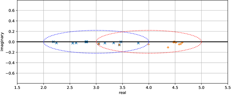
Figure 5. Ritz values found within two overlapping elliptical contours in the $Z$-plane for the microstructured fiber.

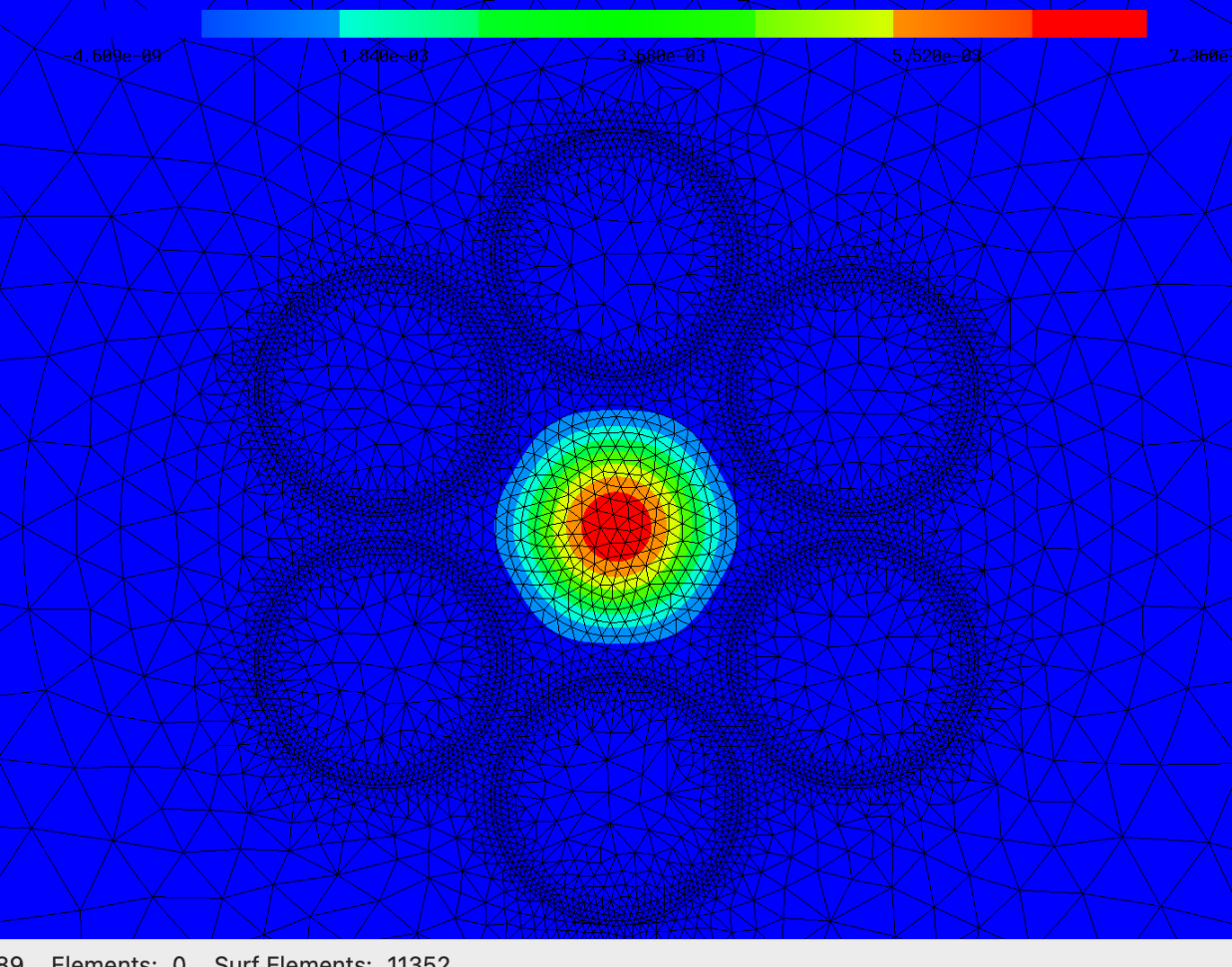
(a) $2.186-\hat{\imath}\,2.1\times 10^{-6}$

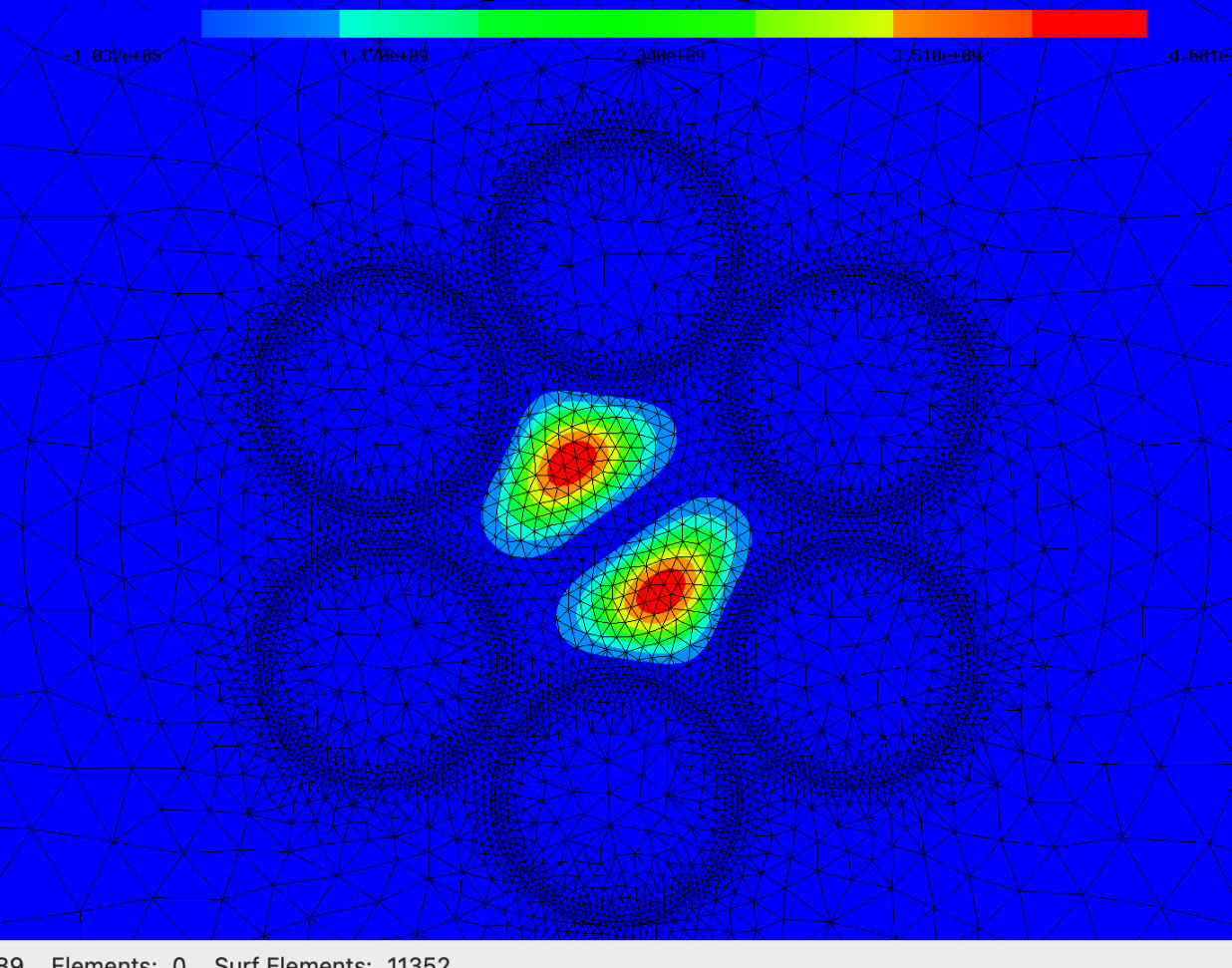
(b) $3.469-\hat{\imath}\,7.0\times 10^{-5}$

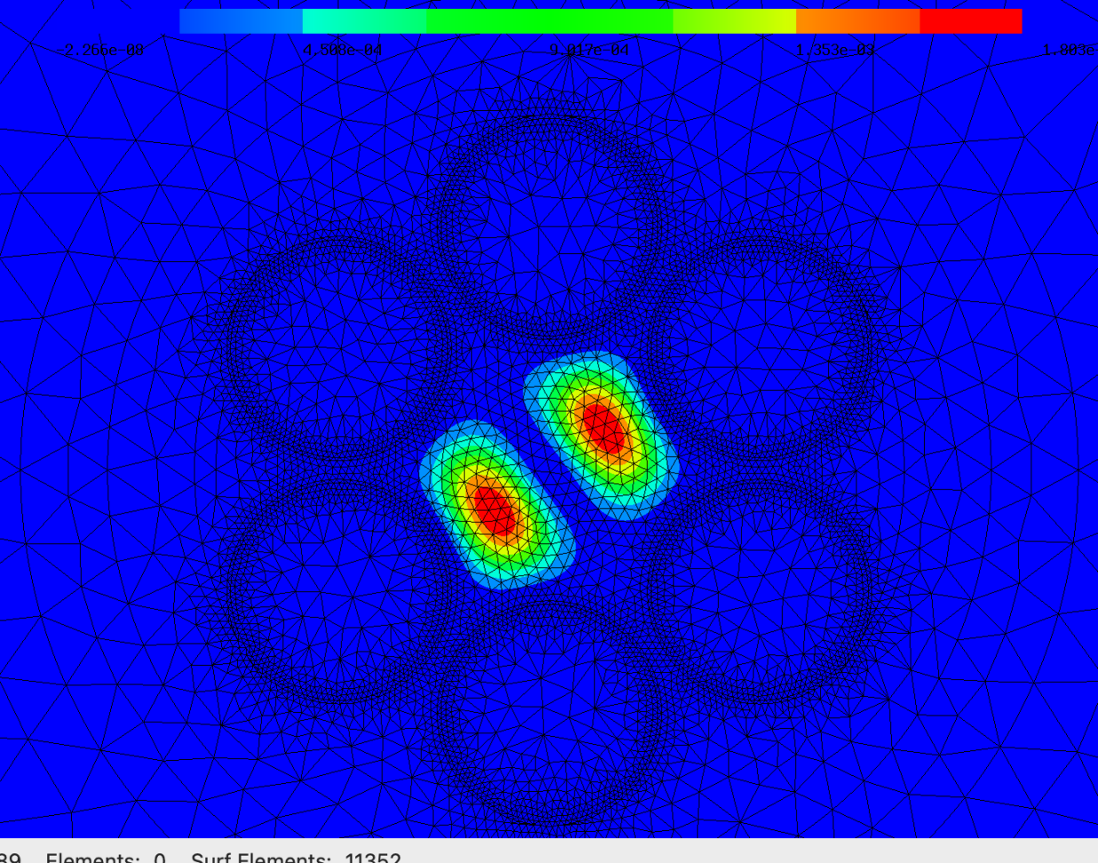
(c) $3.469-\hat{\imath}6.4\times 10^{-5}$

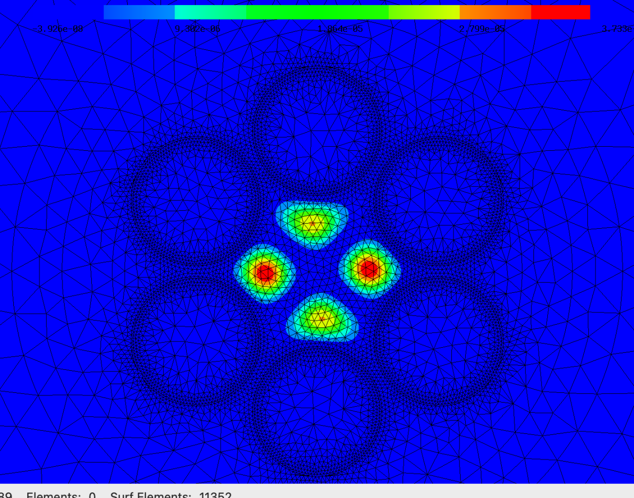
(d) $4.637-\hat{\imath}\,2.4\times 10^{-3}$

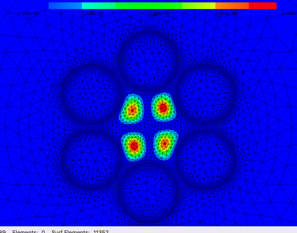
(e) $4.637-\hat{\imath}\,2.2\times 10^{-3}$

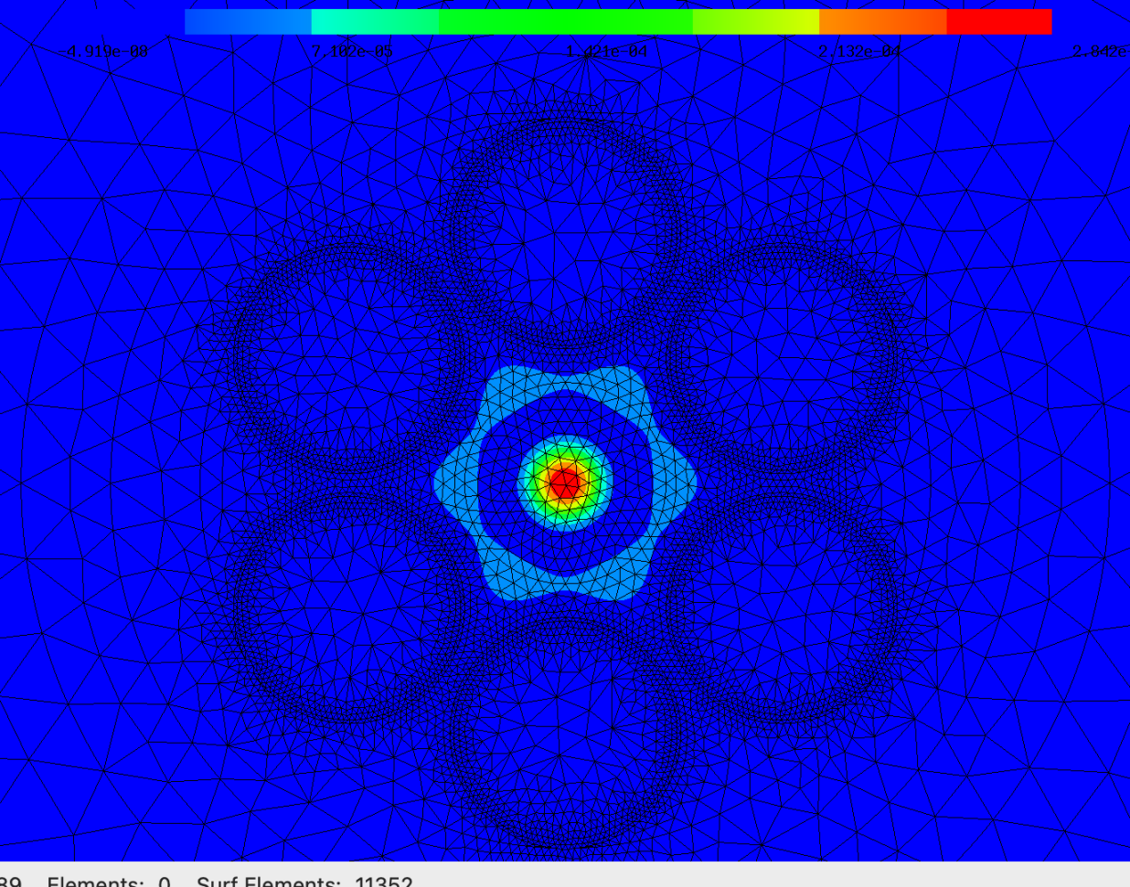
(f) $4.961-\hat{\imath}\,8.6\times 10^{-4}$

Figure 6. Intensities of computed modes are shown zoomed into a rectangle covering the hollow core (the region $r<R_{\mathrm{core}}$ of Figure 1), labeled with their approximate nondimensional $Z$ values for $\lambda=10^{-6}$m.

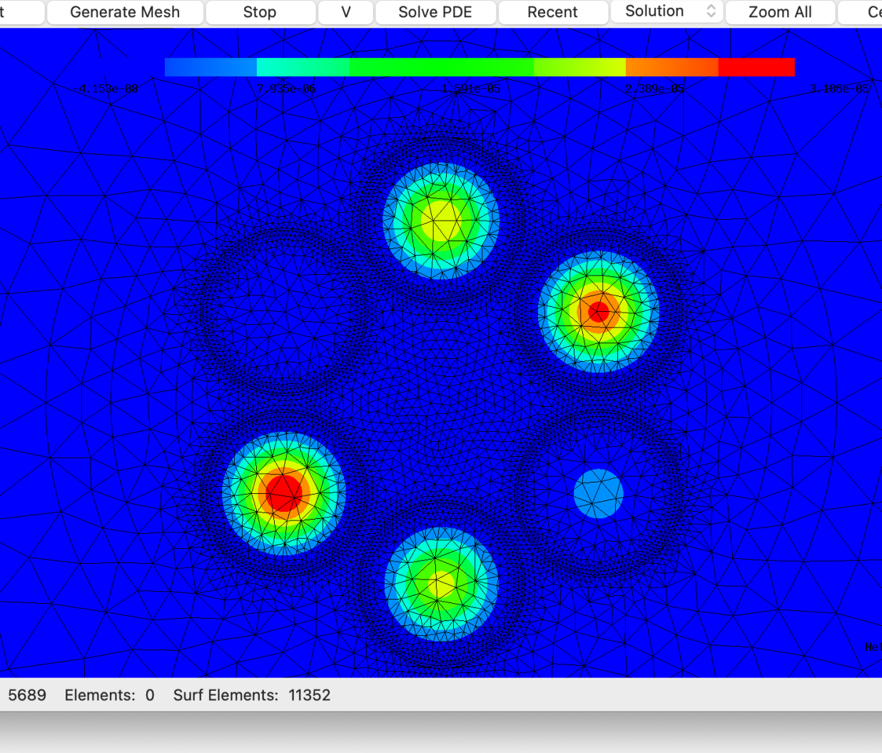
(a) $2.802-\hat{\imath}\,2.4\times 10^{-3}$

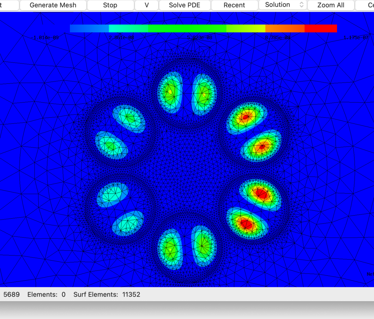
(b) $4.481-\hat{\imath}\,7.4\times 10^{-3}$

Figure 7. Examples of high-loss non-core modes observed in computations are shown. Six modes similar to that in Fig. 7(a) and twelve modes similar to that in Fig. 7(b) were observed.

Next, we apply the method verified in Subsection 3.2. As described there, we first apply Algorithm 1 to conduct a preliminary search, followed by further runs to obtain accurately converged eigenvalues. Before we give the results of the preliminary search, recall from Figure 3 that discretizations of the essential spectrum can seep into circular contours close to the origin, wasting computational resources on irrelevant modes. In the current example, we show how to avoid this using elliptical contours. Since the eigenvalues arising from the essential spectrum are expected to subtend a negative acute angle with the real axis at the origin, an elliptical contour (by increasing its eccentricity) can avoid them better than circular contours. This is seen in our results of Figure 5 (where we do not see the signs of essential spectrum that we saw in Figure 3). The Ritz values in this figure were output after a few iterations of Algorithm 1 employing the quadrature formula in (6) with two overlapping ellipses centered at $y=3$ and $y=4$, each with $\gamma=1$, $\rho^{-1}=0.8$, $N=10$, and $m=20$. For this figure, the discrete nonlinear eigenproblem was built using $\lambda=1000$ nm, $\alpha=5$ (the default value of $\alpha$ used for all computations in this section), $p=10$, and a mesh with curved elements sufficient to resolve the thin geometrical features. A part of this mesh is visible in Figure 6. We will refine this mesh many times over for some computations below.

Let us now focus on one of these Ritz values near $Z=2.18$ and run Algorithm 1 to convergence using a tight circular contour that excludes all other Ritz values. The corresponding computed leaky mode is shown in Figure 6(a) for the case $p=20$. Although the algorithm quickly converges for various discretization parameters to (visually) the same eigenmode, we observed a surprisingly large preasymptotic regime where the imaginary part of the eigenvalues varied significantly even as meshes were made finer and polynomial degrees were increased. Convergence was observed only after crossing this preasymptotic regime. We proceed to describe its implication on estimating mode loss, an important practical quantity of interest. Confinement loss (CL) in fibers, usually expressed in decibels (dB) per meter, refer to $-10\log_{10}(\wp(1)/\wp(0))$ where $\wp(z)$ is the power at the length $z$ meters. For a leaky mode, viewing $\wp(z)$ as proportional to $|e^{-\hat{\imath}\beta z}|^{2}$, its CL can be estimated (see e.g., [24, pp. 213]) from the propagation constant by CL$=-20\log_{10}e^{-\mathop{\mathrm{imag}}\beta}=20\mathop{\mathrm{imag}}\beta/\ln(10)$.

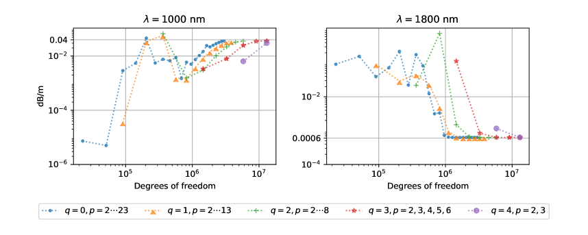
Figure 8. Computed confinement losses for the hollow core fiber show prominent preasymptotic variations for lower mesh refinements ($q$) and polynomial degrees $(p)$.

We computed CL from the eigenvalues obtained for various $h$ and $p$. To systematically vary $h$, we started with an initial mesh (part of which is visible in Figures 6 and 7) and performed successive refinements. One refinement divides each triangular element in the mesh into four (and the four are exactly congruent when the element is not curved). Thus, the mesh after ${q}$ refinements has a grid size $2^{-{q}}$ times smaller than the starting mesh. The results for various ${q}$ and degrees $p$ are in Figure 8. Each dotted curve there represents many computations performed on a fixed mesh (i.e., fixed ${q}$-value) for increasing values of the degree $p$. For the case of $\lambda=1000$ nm we observe that the computed CL values appear to converge to around 0.04 dB/m, but only well after a few millions of degrees of freedom. In particular, the CL values computed using discretizations with under one million degrees of freedom are off by a few orders of magnitude. We also observe that quicker routes (more efficient in terms of degrees of freedom) to converged CL values are offered by the choices that use higher degrees $p$ (rather than higher mesh refinements ${q}$). The second plot in Figure 8 shows similar results for the case of operating wavelength $\lambda=1800$ nm. In this case, CL seems to be largely overestimated in a preasymptotic regime, but computations using upwards of several millions of degrees of freedom agree on a value of around CL$=0.0006$ dB/m, as seen from Figure 8.

We have also confirmed that our results remain stable in the asymptotic convergent regime as we vary the PML parameters. Table 1 shows an example of results from one such parameter variation study. Remaining in the above-mentioned case of $\lambda=1800$ nm, we focus on how one of the points (for $q=1,p=10$) in the second plot of Figure 8 varies under changes in PML width and strength. Table 1 displays how the computed CL values vary slightly around $0.000628$ dB/m.

		CL (dB/m)
PML width ($\mu$m)	Degrees of freedom	$\alpha=1$	$\alpha=5$	$\alpha=10$
50	2270641	0.000630	0.000629	0.000629
100	2603121	0.000628	0.000628	0.000629
150	2482041	0.000628	0.000628	0.000628

Table 1. Computed confinement losses for varying PML widths and PML parameters $\alpha$ (fixing $q=1$ and $p=10$).

We conclude this section by presenting visualizations of modes through plots of their intensities (which are proportional to the square moduli) of the computed modes. In Figure 6, in addition to the fundamental mode (Figure 6(a)), we display a few further higher order modes we found (Figures 6(b)—6(f)). Although these higher order modes exhibit good core localization, their CL values are higher than the fundamental mode. This hollow core structure also admits modes that support transmission outside of the central hollow core, such as those shown in Figure 7. They are, however, much more lossy than the fundamental mode.

5. Proofs

A basic ingredient for proving Theorem 2 is the next result which can be found proved using differential equations in [9, Chapter 7]. We give a different elementary proof. Let $N$ denote a $k\times k$ nilpotent matrix with zero entries except for ones on the first superdiagonal, and let $I$ be the $k\times k$ identity matrix. Then $J=\lambda I+N$ is a $k\times k$ Jordan matrix.

Lemma 7.

A sequence $v_{0},v_{1},\ldots v_{k-1}$ in $\mathbb{C}^{n}$ is a nontrivial Jordan chain of a nonlinear eigenvalue $\lambda$ of $P(z)$ in the sense of definition (8), if and only if $v_{0}\neq 0$ and $V=[v_{0},v_{1},\ldots v_{k-1}]\in\mathbb{C}^{n\times k}$ satisfies

$$\sum_{i=0}^{d}A_{i}VJ^{i}=0.$$ (36)

Proof.

Let $s_{i\ell}=(\begin{smallmatrix}i\\ \ell\end{smallmatrix})\,\lambda^{i-\ell}A_{i}VN^{\ell}$. The sum in (36) can be alternately expressed as

$$\sum_{i=0}^{d}A_{i}VJ^{i} =\sum_{i=0}^{d}A_{i}V\sum_{\ell=0}^{\min(i,k-1)}\begin{pmatrix}i\\ \ell\end{pmatrix}\lambda^{i-\ell}N^{\ell}=\left(\sum_{i=0}^{k-1}+\sum_{i=k}^{d}\right)\sum_{\ell=0}^{\min(i,k-1)}s_{i\ell}$$

$$=\left(\sum_{i=0}^{k-1}\sum_{\ell=0}^{i}+\sum_{i=k}^{d}\sum_{\ell=0}^{k-1}\right)s_{i\ell}=\left(\sum_{\ell=0}^{k-1}\sum_{i=\ell}^{k-1}+\sum_{\ell=0}^{k-1}\sum_{i=k}^{d}\right)s_{i\ell}=\sum_{\ell=0}^{k-1}\sum_{i=\ell}^{d}s_{i\ell}.$$

Observing the connection between the summands and the derivatives of $P(\lambda)$,

$$\sum_{i=\ell}^{d}s_{i\ell}=\frac{1}{\ell!}\big{[}\,0\cdots 0_{\ell},\;P^{(\ell)}(\lambda)v_{0},\ldots,P^{(\ell)}(\lambda)v_{k-1-\ell}\big{]}.$$

where $0\cdots 0_{\ell}$ denote $\ell$ zero columns. Hence (36) is equivalent to

$$\sum_{\ell=0}^{k-1}\frac{1}{\ell!}\big{[}\,0\cdots 0_{\ell},\;P^{(\ell)}(\lambda)v_{0},\ldots,P^{(\ell)}(\lambda)v_{k-1-\ell}\big{]}=0.$$

Since the $j$th column of the left hand side is the same as $\sum_{\ell=0}^{j}(1/\ell!)P^{(\ell)}(\lambda)v_{j-\ell},$ these equations are exactly the same as the defining requirements for $v_{i}$ to form a Jordan chain for a nonlinear eigenvalue $\lambda$, per definition (8). ∎

Proof of Theorem 2.

Let $\lambda$ be a nonlinear eigenvalue enclosed by $\varGamma$. Then, by Lemma 7, $v_{0},v_{1},\ldots v_{k-1}$ in $\mathbb{C}^{n}$ is an associated (right) Jordan chain if and only if equation (36) holds, which is the same as the last equation of the following system

$$\begin{bmatrix}0&I&&\\ \vdots&&\ddots&\\ 0&&&I\\ A_{0}&A_{1}&\cdots&A_{d-1}\end{bmatrix}\underbrace{\begin{bmatrix}V\\ VJ\\ \vdots\\ VJ^{d-1}\end{bmatrix}}_{\mathcal{V}}=\begin{bmatrix}I&\\ &\ddots\\ &&I&\\ &&&-A_{d}\end{bmatrix}\underbrace{\begin{bmatrix}V\\ VJ\\ \vdots\\ VJ^{d-1}\end{bmatrix}}_{\mathcal{V}}J.$$ (37)

Considering that the remaining equations of (37) trivially hold, we have shown that (36) holds if and only if (37) holds. Let $\mathcal{V}_{i}\in\mathbb{C}^{nd}$ denote the $(i+1)^{\text{th}}$ column of the $nd\times k$ matrix $\mathcal{V}$ indicated in (37), so that $\mathcal{V}=[\mathcal{V}_{0},\;\mathcal{V}_{1},\ldots,\mathcal{V}_{k-1}]$. Since (37) is the same as $\mathcal{A}\mathcal{V}=\mathcal{B}\mathcal{V}J$, or equivalently (see the characterization (9a))

$$(\mathcal{A}-\lambda\mathcal{B})\mathcal{V}_{0}=0,\;\text{ and }(\mathcal{A}-\lambda\mathcal{B})\mathcal{V}_{i}=\mathcal{B}\mathcal{V}_{i-1}\;\text{ for }i=1,2,\ldots,k-1,$$

i.e., the columns of $\mathcal{V}$ form a Jordan chain for the linear matrix pencil $\mathcal{A}-\lambda\mathcal{B}$. Noting that $v_{i}=F\mathcal{V}_{i}$, we have thus shown that $\mathcal{V}_{0},\ldots,\mathcal{V}_{k-1}\in\mathbb{C}^{nd}$ is a Jordan chain for $\mathcal{A}-\lambda\mathcal{B}$ if and only if its first blocks, namely $v_{0},v_{1},\ldots v_{k-1}$ in $\mathbb{C}^{n},$ form a Jordan chain for $P(\lambda)$. Since any $x\in\mathbb{C}^{n}$ falling within the algebraic eigenspace of the nonlinear eigenvalue $\lambda$ is a linear combination of such chains $\{v_{i}\}$, the proof of the first item of the theorem is complete.

To prove the second item of the theorem, we start as above with the nonlinear eigenvalue $\lambda,$ but now proceed with its left Jordan chain $\tilde{v}_{0},\tilde{v}_{1},\ldots\tilde{v}_{k-1}\in\mathbb{C}^{n}.$ The second definition of (8) implies $\sum_{l=0}^{j}(l!)^{-1}\tilde{P}^{(l)}(\bar{\lambda})\tilde{v}_{j-l}=0$ where $\tilde{P}(z)=\sum_{j=0}^{d}z^{j}A_{j}^{*}$. Applying Lemma 7 to $\tilde{P}(z)$, we find that $\tilde{V}=[\tilde{v}_{0},\tilde{v}_{1},\ldots\tilde{v}_{k-1}]\in\mathbb{C}^{n\times k}$ satisfies

$$\sum_{i=0}^{d}A_{i}^{*}\tilde{V}\bar{J}^{i}=0.$$ (38)

Simple calculations show that (38) holds if and only if

$$\begin{bmatrix}0&\cdots&0&A_{0}^{*}\\ I&\ddots&\vdots&\vdots\\ &\ddots&0&A_{d-2}^{*}\\ &&I&A_{d-1}^{*}\\ \end{bmatrix}\begin{bmatrix}W_{0}\\ \vdots\\ W_{d-2}\\ \tilde{V}\end{bmatrix}=\begin{bmatrix}I&\\ &\ddots\\ &&I&\\ &&&-A_{d}^{*}\end{bmatrix}\begin{bmatrix}W_{0}\\ \vdots\\ W_{d-2}\\ \tilde{V}\end{bmatrix}\bar{J}$$ (39)

with $W_{d-i}=-\sum_{j=0}^{i-1}A^{*}_{d-j}\tilde{V}\bar{J}^{i-1-j}$ for $i=2,\ldots d$. Taking the conjugate transpose of both sides of (39), we find that $\tilde{\mathcal{V}}^{*}=[W_{0}^{*},\cdots,W_{d-2}^{*},\tilde{V}^{*}]\in\mathbb{C}^{k\times nd}$ satisfies $\tilde{\mathcal{V}}^{*}\mathcal{A}=J^{\prime}\tilde{\mathcal{V}}^{*}\mathcal{B},$ an identity which when written using the columns $\tilde{\mathcal{V}}_{i}\in\mathbb{C}^{nd}$ of $\tilde{\mathcal{V}}=[\tilde{\mathcal{V}}_{0},\ldots,\tilde{\mathcal{V}}_{k-1}]$ reads

$$\tilde{\mathcal{V}}_{0}^{*}(\mathcal{A}-\lambda\mathcal{B})=0,\text{ and }\tilde{\mathcal{V}}_{i}^{*}(\mathcal{A}-\lambda\mathcal{B})=\tilde{\mathcal{V}}_{i-1}^{*}\mathcal{B}.$$

Keeping (9b) in view, the above equivalences have thus shown that the columns of $\tilde{\mathcal{V}}$ form a left Jordan chain of $\mathcal{A}-\lambda\mathcal{B}$ if and only if the the columns of the last block of $\tilde{\mathcal{V}}$, namely $L\tilde{\mathcal{V}}=\tilde{V}=[\tilde{v}_{0},\ldots,\tilde{v}_{k-1}]$ form the left Jordan chain of $\lambda$ as a nonlinear eigenvalue of $P(z)$. ∎

Proof of Theorem 4.

The given $X$ satisfies $(z\mathcal{B}-\mathcal{A})X=Y.$ In block component form, this yields

$$zX_{i-1}-X_{i}=Y_{i-1},\qquad i=1,2,\ldots,d-1,$$ (40a)

$$-A_{0}X_{0}-A_{1}X_{1}-\dots-A_{d-2}X_{d-2}-(zA_{d}+A_{d-1})X_{d-1}=Y_{d-1}.$$ (40b)

Clearly (40a) is the same as (15b). Moreover, the $i^{\text{th}}$ equation of (40a), when combined with the $(i-1)^{\text{th}}$ equation of (40a), yields $X_{i}=zX_{i-1}-Y_{i-1}=z(zX_{i-2}-Y_{i-2})-Y_{i-1}.$ This process can be recursively continued to get

$$X_{i}=z^{i}X_{0}-\sum_{j=0}^{i-1}z^{i-1-j}Y_{j},\qquad i=1,2,\ldots,d-1.$$

Substituting these expressions for $X_{i}$ for $i\geq 1$ into (40b), we obtain

$$\sum_{i=0}^{d-1}A_{i}\bigg{(}z^{i}X_{0}-\sum_{j=0}^{i-1}z^{i-1-j}Y_{j},\bigg{)}=-Y_{d-1}-zA_{d}\bigg{(}z^{d-1}X_{0}-\sum_{j=0}^{d-2}z^{d-2-j}Y_{j}\bigg{)}.$$

Moving the term with $z^{d}$ from right to left, we identify a group of terms that sum to $P(z)X_{0}$. Sending all the remaining terms on the left to the right, simplifying, and applying $P(z)^{-1}$ to both sides, we obtain (15a).

For proving (16), let us rewrite the equation $(z\mathcal{B}-\mathcal{A})^{*}X=W$ as the system of equations

$$\bar{z}{\tilde{X}}_{0}-A_{0}^{*}{\tilde{X}}_{d-1} =W_{0}$$ (41a)

$$-{\tilde{X}}_{i-1}+\bar{z}{\tilde{X}}_{i}-A_{i}^{*}{\tilde{X}}_{d-1} =W_{i},\qquad i=1,2,\ldots,d-2,$$ (41b)

$$-{\tilde{X}}_{d-2}-(\bar{z}A_{d}^{*}+A_{d-1}^{*}){\tilde{X}}_{d-1} =W_{d-1},$$ (41c)

Multiply (41b) by $\bar{z}^{i}$ and add up all the equations of (41a)–(41b). Then observe that all terms of the type $-\bar{z}^{i}\tilde{X}_{i-1}$ telescopically cancel off in the resulting sum, yielding

$$\bar{z}^{d-1}{\tilde{X}}_{d-2}=W_{0}+\bar{z}W_{1}+\bar{z}^{2}W_{2}+\cdots+\bar{z}^{d-2}W_{d-2}+(A_{0}^{*}+\bar{z}A_{1}^{*}+\cdots+\bar{z}^{d-2}A_{d-2}^{*}){\tilde{X}}_{d-1}.$$

Using (41c) to eliminate ${\tilde{X}}_{d-2}$ from the last equation and rearranging, we have

$$\sum_{j=0}^{d-1}\bar{z}^{j}W_{j}+P(z)^{*}{\tilde{X}}_{d-1}=0,$$

which immediately yields the expression for ${\tilde{X}}_{d-1}$ in (16a). The expressions for the remaining ${\tilde{X}}_{i}$ in (16) follow from (41c) and (41b), respectively. ∎

6. Conclusion

We have presented a new technique to compute collections of transverse leaky modes of optical fibers with complex microstructure by combining advances in contour integral eigensolvers and frequency-dependent PML. The frequency-dependent PML is not yet widely used for resonance computations due to the difficulties in solving the resulting nonlinear eigenproblem. The new avenue we presented using Algorithm 1 makes it a viable computational option when a few resonance values (enclosed in a given contour) is of interest.

Algorithm 1 is applicable more generally to solve for clusters of nonlinear eigenvalues of the polynomial type arising from any application. The efficiencies in the algorithm were gained by circumventing the typical large inverses arising from linearization of the polynomial eigenproblem.

We have exploited FEAST’s flexibility with contours to design ellipses that effectively probe wanted resonances without interference from the deformed essential spectrum. The algorithm also eliminates unwanted eigenfunctions supported in the PML region by sending them to the eigenspace of infinity.

While confinement loss values for some fiber geometries (such as that in Subsection 3.2) can be computed easily and fast, the antiresonant fiber we considered in Section 4 presented a preasymptotic regime, which was surprisingly large for a two-dimensional structure, where computed loss values vary by orders of magnitude. By reporting this in detail, we hope to bring more awareness of this issue to those estimating losses of similar structures with thin filaments.

Acknowledgements

We gratefully acknowledge extensive discussions with Dr. Jacob Grosek (Directed Energy, Air Force Research Laboratory, Kirtland, NM) on practical issues with the accurate computation of transverse modes of optical fibers and with Dr. Markus Wess (ENSTA, Paris) on his dissertation research. This work was supported in part by AFOSR grant FA9550-19-1-0237, AFRL Cooperative Agreement 18RDCOR018, and NSF grant DMS-1912779.

References

- [1] J. C. Araujo-Cabarcas and C. Engström, On spurious solutions in finite element approximations of resonances in open systems, Computers and Mathematics with Applications, 74 (2017), pp. 2385–2402.
- [2] M. Abramowitz and I.E. Stegun, editors, Handbook of Mathematical Functions With Formulas, Graphs, and Mathematical Tables, Applied Mathematics Series, U.S. Department of Commerce National Bureau of Standards, Washington, D.C., 55 (1972), pp. 358–365.
- [3] J.-P. Berenger, A perfectly matched layer for the absorption of electromagnetic waves, J. Comput. Phys., 114 (1994), pp. 185–200.
- [4] W. C. Chew and W. H. Weedon, A 3D perfectly matched medium from modified Maxwell’s equations with stretched coordinates, Microwave and Optical Technology Letters, 7 (1994), pp. 599–604.
- [5] F. Collino and P. Monk, The perfectly matched layer in curvilinear coordinates, SIAM J. Sci. Comput., 19 (1998), pp. 2061–2090 (electronic).
- [6] E. B. Davies, Linear operators and their Spectra, Cambridge University Press, 2007.
- [7] D. Drake, J. Gopalakrishnan, T. Goswami, and J. Grosek, Simulation of optical fiber amplifier gain using equivalent short fibers, Computer Methods in Applied Mechanics and Engineering, 360 (2020), p. 112698.
- [8] B. Gavin, A. Miȩdlar, and E. Polizzi, FEAST eigensolver for nonlinear eigenvalue problems, Journal of Computational Science, 27 (2018), pp. 107–117.
- [9] I. Gohberg, P. Lancaster, and L. Rodman, Matrix Polynomials, Classics in Applied Mathematics (republished in 2009), SIAM, Philadelphia, 1982.
- [10] J. Gopalakrishnan, L. Grubišić, and J. Ovall, Spectral discretization errors in filtered subspace iteration, Mathematics of Computation, 89 (2020), pp. 203–228.
- [11] J. Gopalakrishnan, L. Grubišić, J. Ovall, and B. Q. Parker, Analysis of FEAST spectral approximations using the DPG discretization, Computational Methods in Applied Mathematics, 89 (2020), pp. 203–228.
- [12] J. Gopalakrishnan, S. Moskow, and F. Santosa, Asymptotic and numerical techniques for resonances of thin photonic structures, SIAM J. Appl. Math., 69 (2008), pp. 37–63.
- [13] S. Güttel, E. Polizzi, P. T. P. Tang, and G. Viaud, Zolotarev quadrature rules and load balancing for the FEAST eigensolver, SIAM J. Sci. Comput., 37 (2015), pp. A2100–A2122.
- [14] S. Güttel and F. Tisseur, The nonlinear eigenvalue problem, Acta Numerica, 26 (2017), pp. 1–26.
- [15] T. Kato, Perturbation theory for linear operators, Classics in Mathematics, Springer-Verlag, Berlin, 1995.
- [16] J. Kestyn, E. Polizzi, and P. T. P. Tang, FEAST eigensolver for non-Hermitian problems, SIAM J. Sci. Comput., 38 (2016), pp. S772–S799.
- [17] S. Kim and J. E. Pasciak, The computation of resonances in open systems using a perfectly matched layer, Mathematics of Computation, 78 (2009), pp. 1375–11398.
- [18] A. N. Kolyadin, A. F. Kosolapov, A. D. Pryamikov, A. S. Biriukov, V. G. Plotnichenko, and E. M. Dianov, Light transmission in negative curvature hollow core fiber in extremely high material loss region, Optics Express, 21 (2013), pp. 9514–9519.
- [19] P. Kravanja and M. V. Barel, Computing the Zeros of Analytic Functions, Springer–Verlag, 2000.
- [20] D. Marcuse, Theory of Dielectric Optical Waveguides, Academic Press, 1991.
- [21] L. Nannen and M. Wess, Computing scattering resonances using perfectly matched layers with frequency dependent scaling functions, BIT Numer Math, 58 (2018), pp. 373–395.
- [22] F. Poletti, Nested antiresonant nodeless hollow core fiber, Optics Express, 22 (2014), pp. 23807–23828.
- [23] E. Polizzi, A density matrix-based algorithm for solving eigenvalue problems, Phys. Rev. B 79, 79 (2009), p. 115112.
- [24] G. A. Reider, Photonics: An introduction, Springer, Switzerland, 2016.
- [25] B. Simon, Resonances in n-body quantum systems with dilatation analytic potentials and the foundations of time-dependent perturbation theory, Ann. of Math., (1973).
- [26] J. Schöberl, NETGEN — An advancing front 2D/3D-mesh generator based on abstract rules, Comput Visual Sci, 1 (1997), pp. 41-52.
- [27] J. Schöberl et al, NGSolve, https://ngsolve.org, last retrieved April 21, 2021. An open source high-performance multiphysics finite element software.
- [28] F. Tisseur and K. Meerbergen, The quadratic eigenvalue problem, SIAM Rev., 43 (2001), pp. 235–286.
- [29] M. Wess, Frequency-Dependent Complex-Scaled Infinite Elements for Exterior Helmholtz Resonance Problems, PhD thesis, Technical University of Vienna, 2020.
- [30] F. Yu and J. Knight, Negative curvature hollow core optical fiber, IEEE J. Sel. Topics Quantum Electron, 22 (2016), pp. 1–11.