KUNS-2865

KYUSHU-HET-225

KANAZAWA-21-04

Pseudo-Nambu-Goldstone Dark Matter Model
Inspired by Grand Unification

Yoshihiko Abe¹, Takashi Toma^2,3, Koji Tsumura⁴, Naoki Yamatsu⁴

¹Department of Physics, Kyoto University, Kyoto 606-8502, Japan
²Institute of Liberal Arts and Science,
Kanazawa University, Kakuma-machi, Kanazawa, 920-1192 Japan
³ Institute for Theoretical Physics, Kanazawa University, Kanazawa 920-1192, Japan ⁴Department of Physics, Kyushu University,
744 Motooka, Nishi-ku, Fukuoka, 819-0395, Japan

1 Introduction

The existence of dark matter (DM) has been confirmed by several astronomical observations such as spiral galaxies [1, 2], gravitational lensing [3], cosmic microwave background [4], and collision of bullet cluster [5]. There are no viable DM candidates in the Standard Model (SM), so the identification of DM plays an important role in particle physics as well as cosmology.

Due to the lack of understanding the nature of DM, there are a lot of DM candidates. One of the candidates is so-called Weakly Interacting Massive Particle (WIMP). To realize the the relic abundance of DM, the WIMP mass is expected to the range of $\mathcal{O}(10)$ GeV to $\mathcal{O}(100)$ TeV. Further, since the WIMPs have non-gravitational interaction, the direct and indirect detections are expected, but there are still no clear signals of WIMPs, which lead to the strong constraint for WIMP mass and interactions, especially from the direct detection.

Several mechanisms in WIMP DM models are proposed to avoid the severe constrains from the direct detection by considering e.g., a fermion DM with pseudo-scalar interactions [6, 7, 8, 9, 10, 11] and a pseudo-Nambu-Goldstone boson (pNGB) DM [12, 13, 14, 15, 16, 17, 18, 19, 20, 21]. Usually, in pNGB DM models, additional global $U(1)$ symmetry is assumed in an ad hoc manner.

In Refs. [19, 20], a pNGB DM model is proposed based on $G_{\rm SM}\times U(1)_{B-L}$ gauge groups, where $G_{\rm SM}:=SU(3)_{C}\times SU(2)_{L}\times U(1)_{Y}$. Two complex scalars with $Q_{B-L}=+1$ and $+2$, denoted as $S$ and $\Phi$, and three right-handed neutrinos due to the gauge anomaly cancellation are introduced. The gauge symmetry is spontaneously broken via the nonvanishing vacuum expectation value (VEV) of the scalar fields $S$ and $\Phi$ as below:

$$G_{\rm SM}\times U(1)_{B-L}\ {\longrightarrow}\ G_{\rm SM}.$$ (1.1)

The results in the model are summarized below. The DM direct detection cross section is naturally suppressed as the same as other pNGB DM models. The pNGB can decay through the new high scale suppressed operators, but the pNGB has a lifetime long enough to be a DM in the wide range of the parameter space of the model. The thermal relic abundance of pNGB DM can be fit with the observed value against the constraints on the DM decays from the cosmic-ray observations.

From other viewpoints, the charge quantization of $U(1)_{Y}$, the gauge anomaly cancellation of $G_{\rm SM}$, and the almost SM gauge coupling unification even in non-supersymmetric SM seem to imply the existence of grand unification [22]. The unification scale is expected to be $\mathcal{O}(10^{15}-10^{18})$ GeV, where the lower bound comes from the current non-observation of the nucleon decay [23] and the upper bound comes from the Planck scale. Also, the tiny neutrino masses from the neutrino oscillation data seem to suggest an intermediate scale $\mathcal{O}(10^{10}-10^{14})$ GeV through a see-saw mechanism [24].

In this paper, we propose an $SO(10)$ pNGB DM model in the framework of grand unified theories (GUTs). Each Weyl fermion in ${\bf 16}$ of $SO(10)$ contains one generation of quarks and leptons, which includes a right-handed neutrino [25]. The SM Higgs and two complex scalar fields $S$ and $\Phi$ in Refs. [19, 20] are assigned to a scalar field in ${\bf 10}$, ${\bf 16}$, and ${\bf\overline{126}}$ of $SO(10)$, respectively. There are several symmetry breaking patterns of $SO(10)$ to $G_{\rm SM}\times U(1)_{B-L}$ as below.

$$SO(10)\ {\longrightarrow}\ G_{I}\ {\longrightarrow}\ G_{\rm SM}\times U(1)_{B-L}.$$ (1.2)

where $G_{I}$ stands for the intermediate gauge group such as the Pati-Salam gauge group $G_{\rm PS}:=SU(4)_{C}\times SU(2)_{L}\times SU(2)_{R}$ [26] and a left-right gauge group $G_{\rm LR}:=SU(3)_{C}\times SU(2)_{L}\times SU(2)_{R}\times U(1)_{B-L}$ [27, 28]. We mainly focus on the case of $G_{I}=G_{\rm PS}$, but we also consider the possibility for such as $G_{I}=G_{\rm LR}$, where the cases are not favored for a pNGB DM model under our assumption and experimental constraints. (For more information about GUT model building in general, see, e.g., Refs. [29, 30].)

We discuss the following three things. First, the value of the gauge kinetic mixing between $U(1)_{Y}$ and $U(1)_{B-L}$ is a free parameter in e.g., the non-GUT pNGB DM models [19, 20], while that is determined mainly by the GUT gauge group in $SO(10)$ models. Second, gauge coupling unification can be achieved due to the contribution from the additional scalar fields that contain a DM candidate. Then the intermediate scale $M_{I}$, the unification scale $M_{U}$, and the gauge coupling constant of $U(1)_{B-L}$ are fixed by using the renormalization group equations (RGEs) for gauge coupling constants. Third, the mass of the pNGB in the $SO(10)$ pNGB DM model is limited to be $\mathcal{O}(10-100)$ GeV from experimental constraints.

The paper is organized as follows. In Sec. 2, we introduce the $SO(10)$ pNGB DM model. In Sec. 3, we find gauge coupling unification determines mass scales and gauge coupling constants of the model. In Sec. 4, the constraints from experiments are discussed. Section 5 is devoted to summary and discussions.

2 The model

The model consists of an $SO(10)$ gauge field $\mathsf{A}_{\mu}$, fermions in 16 of $SO(10)$, a real scalar field in ${\bf 210}$ of $SO(10)$, and complex scalar fields in ${\bf 10}$, ${\bf 16}$ and ${\bf\overline{126}}$ of $SO(10)$. The $SO(10)$ gauge field contains $G_{\rm SM}$ and $U(1)_{B-L}$ gauge fields. Each fermion in 16 of $SO(10)$ corresponds to quarks and leptons. Scalar fields in ${\bf 10}$, ${\bf 16}$, and ${\bf\overline{126}}$ of $SO(10)$ include the Higgs $H$, $S$ and $\Phi$, respectively. A scalar field in ${\bf 210}$ of $SO(10)$ is responsible for breaking the $SO(10)$ symmetry to $G_{\rm PS}$. The matter content in the $SO(10)$ model is summarized in Table 1.

	$\mathsf{A}_{\mu}$	$\mathsf{\Psi}_{\bf 16}$	$\mathsf{\Phi}_{\bf 10}$	$\mathsf{\Phi}_{\bf 16}$	$\mathsf{\Phi}_{\overline{\bf 126}}$	$\mathsf{\Phi}_{\bf 210}$
$SO(10)$	${\bf 45}$	${\bf 16}$	${\bf 10}$	${\bf 16}$	${\overline{\bf 126}}$	${\bf 210}$
$SL(2,\mathbb{C})$	$(1/2,1/2)$	$(1/2,0)$	$(0,0)$	$(0,0)$	$(0,0)$	$(0,0)$

Table 1: The matter content in the $SO(10)$ model is shown.

The Lagrangian is given by

$${\cal L} =\sum_{\bf y={\bf 10,16,\overline{126}}}\left(\mathsf{D}_{\mu}\mathsf{\Phi}_{\bf y}\right)^{\dagger}\left(\mathsf{D}^{\mu}\mathsf{\Phi}_{\bf y}\right)+\frac{1}{2}\left(\mathsf{D}_{\mu}\mathsf{\Phi}_{\bf 210}\right)^{T}\left(\mathsf{D}^{\mu}\mathsf{\Phi}_{\bf 210}\right)+\sum_{a=1}^{3}\overline{\mathsf{\Psi}_{\bf 16}^{(a)}}i\cancel{\mathsf{D}}\mathsf{\Psi}_{\bf 16}^{(a)}-\frac{1}{2}\mbox{tr}\left[\mathsf{F}_{\mu\nu}\mathsf{F}^{\mu\nu}\right]$$

$$-\left(\sum_{\bf y=10,\overline{126}}\sum_{a,b}\mathsf{y}_{\bf y}^{(ab)}\mathsf{\Phi}_{\overline{\bf y}}\left(\mathsf{\Psi}_{\bf 16}^{(a)}\mathsf{\Psi}_{\bf 16}^{(b)}\right)_{\bf y}+\mbox{h.c.}\right)-V\left(\left\{\mathsf{\Phi}_{\bf x}\right\}\right),$$ (2.1)

where $\mathsf{D}_{\mu}:=\partial_{\mu}+i\mathsf{g}\mathsf{A}_{\mu}$, $\mathsf{F}_{\mu\nu}:=\partial_{\mu}\mathsf{A}_{\nu}-\partial_{\nu}\mathsf{A}_{\mu}+i\mathsf{g}[\mathsf{A}_{\mu},\mathsf{A}_{\nu}]$. The scalar potential $V\left(\left\{\mathsf{\Phi}_{\bf x}\right\}\right)$ contains quadratic, cubic, and quartic coupling terms, where ${\bf x}={\bf 10,16,\overline{126},210}$.

	$\mathsf{\Psi}_{\bf 16}$
$SO(10)$	${\bf 16}$
	$\psi_{\bf(4,2,1)}$		$\psi_{{\bf(\overline{4},1,2)}}$
$G_{\rm PS}$	${\bf(4,2,1)}$		${{\bf(\overline{4},1,2)}}$
	$Q_{L}$	$L$	$u_{R}^{c}$	$d_{R}^{c}$	$e_{R}^{c}$	$\nu_{R}^{c}$
$SU(3)_{c}$	${\bf 3}$	${\bf 1}$	$\bar{\bf 3}$	$\bar{\bf 3}$	${\bf 1}$	${\bf 1}$
$SU(2)_{L}$	${\bf 2}$	${\bf 2}$	${\bf 1}$	${\bf 1}$	${\bf 1}$	${\bf 1}$
$U(1)_{Y}$	$+1/6$	$-1/2$	$-2/3$	$+1/3$	$+1$	$0$
$U(1)_{B-L}$	$+1/3$	$-1$	$-1/3$	$-1/3$	$+1$	$+1$

Table 2: The content of fermions in the $SO(10)$ model is shown in the $G_{\rm PS}=SU(4)_{C}\times SU(2)_{L}\times SU(2)_{R}$ basis, where the fermions belong to $(1/2,0)$ under $SL(2,\mathbb{C})$. The $U(1)_{B-L}$ charge $Q_{B-L}$ is given by $U(1)(\subset SU(4)/SU(3)$) [30].

We consider the following symmetry breaking patterns of $SO(10)$ broken to $G_{\rm PS}$ at the unification scale $M_{U}$ by the nonvanishing vacuum expectation value (VEV) of the scalar field in ${\bf 210}$ in $SO(10)$, further to $G_{\rm SM}$ at the intermediate scale $M_{I}$ by the VEV of the scalar field in ${\bf\overline{126}}$ in $SO(10)$, where the $M_{U}$ and $M_{I}$ will be determined by gauge coupling unification using the renormalization group equations (RGEs) for the gauge coupling constants in the next section.

$$SO(10) \xrightarrow[]{\hskip 2.84526pt\langle\mathsf{\Phi}_{\bf 210}\rangle\not=0\hskip 2.84526pt}G_{\rm PS}\left(\supset G_{\rm SM}\times U(1)_{B-L}\right)\xrightarrow[]{\hskip 2.84526pt\langle\mathsf{\Phi}_{\bf\overline{126}}\rangle\not=0\hskip 2.84526pt}G_{\rm SM}\xrightarrow[]{\hskip 2.84526pt\langle\mathsf{\Phi}_{\bf 10}\rangle\not=0\hskip 2.84526pt}SU(3)_{C}\times U(1)_{\rm EM},$$ (2.2)

where the dominant contribution for the symmetry breaking from the VEVs are shown. The type of symmetry breaking has been already discussed in e.g., Refs. [25, 32, 33, 34, 31, 35, 36, 37, 38, 39, 40, 41, 42, 43]. The field content of fermion, scalar, and gauge bosons are shown in Tables 2, 3, and 4. (The potential analysis of ${\bf 210}$ in $SO(10)$ has already discussed in e.g., Ref. [44]; $SO(10)$ is broken to $G_{\rm PS}$ for appropriate parameter sets.)

	$\mathsf{\Phi}_{\bf 10}$	$\mathsf{\Phi}_{\bf 16}$	$\mathsf{\Phi}_{\overline{\bf 126}}$
$SO(10)$	${\bf 10}$	${\bf 16}$	$\overline{\bf 126}$
	$\phi_{\bf(1,2,2)}$	$\phi_{\bf(\overline{4},1,2)}$	$\phi_{\bf(\overline{10},1,3)}$
$G_{\rm PS}$	${\bf(1,2,2)}$	${\bf(\overline{4},1,2)}$	${\bf(\overline{10},1,3)}$
	$H$	$S$	$\Phi$
$SU(3)_{c}$	${\bf 1}$	${\bf 1}$	${\bf 1}$
$SU(2)_{L}$	${\bf 2}$	${\bf 1}$	${\bf 1}$
$U(1)_{Y}$	$+1/2$	$0$	$0$
$U(1)_{B-L}$	$0$	$+1$	$+2$

Table 3: The content of scalar fields in the $SO(10)$ model is shown, where the scalars belong to $(0,0)$ under $SL(2,\mathbb{C})$; $\mathsf{\Phi}_{\bf 10}$, $\mathsf{\Phi}_{\bf 16}$ and $\mathsf{\Phi}_{\bf\overline{126}}$ are complex scalar fields. Here we assume all unlisted components of $G_{\rm PS}$ have ${\cal O}(M_{U})$ masses and also all unlisted components of $G_{\rm SM}\times U(1)_{B-L}$ have $\mathcal{O}(M_{I})$ and $\mathcal{O}(M_{U})$ masses, respectively. Other information is the same as in Table 2.

	$\mathsf{A}_{\mu}$
$SO(10)$	${\bf 45}$
	$G_{\mu}^{\prime}$		$W_{\mu}$	$W_{\mu}^{\prime}$
$G_{\rm PS}$	${\bf(15,1,1)}$		${\bf(1,3,1)}$	${\bf(1,1,3)}$
	$G_{\mu}$	$C_{\mu}$	$W_{\mu}$	$Z_{\mu}^{\prime}$
$SU(3)_{c}$	${\bf 8}$	${\bf 1}$	${\bf 1}$	${\bf 1}$
$SU(2)_{L}$	${\bf 1}$	${\bf 1}$	${\bf 3}$	${\bf 1}$
$U(1)_{Y}$	$0$	$0$	$0$	$0$
$U(1)_{B-L}$	$0$	$0$	$0$	$0$

Table 4: The content of gauge fields in the $SO(10)$ model is shown, where the gauge fields belong to $(1/2,1/2)$ under $SL(2,\mathbb{C})$; Other information is the same as in Tables 2 and 3.

2.1 Scalar sector

Here we focus on the scalar potential of SM Higgs and pNGB relevant part that contains scalar fields $H$, $S$, $\Phi$ belonging to ${\bf 10}$, ${\bf 16}$, and ${\bf\overline{126}}$ of $SO(10)$, respectively. We assume that the other components of $\mathsf{\Phi}_{\bf 10}$, $\mathsf{\Phi}_{\bf 16}$ and $\mathsf{\Phi}_{\overline{\bf 126}}$ shown in Table 3 have the intermediate scale or larger masses and they do not contribute $SU(2)_{L}\times U(1)_{Y}$ and $U(1)_{B-L}$ breakings.

From the scalar potential $V\left(\left\{\mathsf{\Phi}_{\bf x}\right\}\right)$ in Eq. (2.1), we extract the terms that contain only $H$, $S$, $\Phi$:

$$V\left(H,S,\Phi\right) =-\frac{\mu_{H}^{2}}{2}|H|^{2}-\frac{\mu_{S}^{2}}{2}|S|^{2}-\frac{\mu_{\Phi}^{2}}{2}|\Phi|^{2}+\frac{\lambda_{H}}{2}|H|^{4}+\frac{\lambda_{S}}{2}|S|^{4}+\frac{\lambda_{\Phi}}{2}|\Phi|^{4}$$

$$+\lambda_{HS}|H|^{2}|S|^{2}+\lambda_{H\Phi}|H|^{2}|\Phi|^{2}+\lambda_{S\Phi}|S|^{2}|\Phi|^{2}-\left(\frac{\mu_{c}}{\sqrt{2}}\Phi^{*}S^{2}+\mbox{c.c.}\right).$$ (2.3)

The quadratic terms $|H|^{2}$, $|S|^{2}$, and $|\Phi|^{2}$ come from $(\mathsf{\Phi}_{\bf 10}\mathsf{\Phi}_{\bf 10})_{\bf 1}$, $(\mathsf{\Phi}_{\bf 16}\mathsf{\Phi}_{\bf 16}^{*})_{\bf 1}$, and $(\mathsf{\Phi}_{\bf\overline{126}}\mathsf{\Phi}_{\bf\overline{126}}^{*})_{\bf 1}$, respectively; the quartic terms $|H|^{4}$, $|S|^{4}$, and $|\Phi|^{4}$ come from $((\mathsf{\Phi}_{\bf 10}\mathsf{\Phi}_{\bf 10})_{\bf 1})^{2}$ and $|(\mathsf{\Phi}_{\bf 10}\mathsf{\Phi}_{\bf 10})_{\bf 54}|^{2}$ $|(\mathsf{\Phi}_{\bf 16}\mathsf{\Phi}_{\bf 16})_{\bf\overline{126}}|^{2}$, and $|(\mathsf{\Phi}_{\bf\overline{126}}\mathsf{\Phi}_{\bf\overline{126}})_{\bf\overline{2772}}|^{2}$, respectively; the quartic terms $|H|^{2}|S|^{2}$, $|H|^{2}|\Phi|^{2}$, and $|S|^{2}|\Phi|^{2}$ come from $(\mathsf{\Phi}_{\bf 10}\mathsf{\Phi}_{\bf 10})_{\bf 1}(\mathsf{\Phi}_{\bf 16}\mathsf{\Phi}_{\bf 16}^{*})_{\bf 1}$, $(\mathsf{\Phi}_{\bf 10}\mathsf{\Phi}_{\bf 10})_{\bf 1}(\mathsf{\Phi}_{\bf\overline{126}}\mathsf{\Phi}_{\bf\overline{126}}^{*})_{\bf 1}$, and $(\mathsf{\Phi}_{\bf 16}\mathsf{\Phi}_{\bf 16}^{*})_{\bf 1}(\mathsf{\Phi}_{\bf\overline{126}}\mathsf{\Phi}_{\bf\overline{126}}^{*})_{\bf 1}$, respectively; the cubic term $\Phi^{*}S^{2}$ comes from $\mathsf{\Phi}_{\bf\overline{126}}^{*}(\mathsf{\Phi}_{\bf 16}\mathsf{\Phi}_{\bf 16})_{\bf\overline{126}}$, where the above subscript such as ${\bf 1}$ and ${\bf 54}$ stands for the product representation of $SO(10)$. This potential is exactly the same as that in Refs. [19, 20].

We assume that the scalar fields $H$, $S$, and $\Phi$ develop the VEVs, which are parameterized by

$$H=\left(\begin{array}[]{c}0\\ \frac{v+h}{\sqrt{2}}\\ \end{array}\right),\ \ \ S=\frac{v_{s}+s+i\eta_{s}}{\sqrt{2}},\ \ \ \Phi=\frac{v_{\phi}+\phi+i\eta_{\phi}}{\sqrt{2}},$$ (2.6)

where $h$, $s$, and $\phi$ are CP-even modes, $\eta_{s}$ and $\eta_{\phi}$ are CP-odd modes, and $v$, $v_{s}$, and $v_{\phi}$ are the VEVs of $H$, $S$, and $\Phi$, respectively. The CP phase of the cubic term $\Phi^{*}S^{2}$ is eliminated by the field redefinition of $\Phi$. In the limit $\mu_{c}\to 0$, there are two independent global $U(1)$ symmetries associated with the phase rotation of $S$ and $\Phi$. For $\mu_{c}\not=0$, the $U(1)$ symmetries are merged to the $U(1)_{B-L}$ (or $U(1)_{X}$) symmetry. Once $U(1)_{B-L}$ is broken, one of two CP-odd modes is absorbed by the $U(1)_{B-L}$ gauge field denoted as $C_{\mu}$, while the other appears as a physical pNGB whose mass is proportional to $\mu_{c}$.

The scalar fields $H$, $S$, $\Phi$ have five modes; three of them are CP-even scalar modes and the other two are CP-odd modes. The mass matrix for the CP-even scalars in the $(h,s,\phi)$ basis is given by

$$M_{\rm even}^{2}=\left(\begin{array}[]{ccc}\lambda_{H}v^{2}&\lambda_{HS}vv_{s}&\lambda_{H\Phi}vv_{\phi}\\ \lambda_{HS}vv_{s}&\lambda_{S}v_{s}^{2}&\lambda_{S\Phi}v_{s}v_{\phi}-\mu_{c}v_{s}\\ \lambda_{H\Phi}vv_{\phi}&\lambda_{S\Phi}v_{s}v_{\phi}-\mu_{c}v_{s}&\lambda_{\Phi}v_{\phi}^{2}+\frac{\mu_{c}v_{s}^{2}}{2v_{\phi}}\\ \end{array}\right).$$ (2.10)

Since the matrix is real and symmetric, it can be diagonalized by a real orthogonal matrix. The gauge eigenstates $(h,s,\phi)$ are related with the mass eigenstates $(h_{1},h_{2},h_{3})$ as

$$\left(\begin{array}[]{c}h\\ s\\ \phi\\ \end{array}\right)=U_{e}\left(\begin{array}[]{c}h_{1}\\ h_{2}\\ h_{3}\\ \end{array}\right),$$ (2.17)

where the approximate form of the real orthogonal matrix and its mixing angle are given by

$$U_{e}\simeq\left(\begin{array}[]{ccc}1&0&\frac{\lambda_{H\Phi}v}{\lambda_{\Phi}v_{\phi}}\\ 0&1&\frac{\lambda_{S\Phi}v}{\lambda_{\Phi}v_{\phi}}\\ -\frac{\lambda_{H\Phi}v}{\lambda_{\Phi}v_{\phi}}&-\frac{\lambda_{S\Phi}v}{\lambda_{\Phi}v_{\phi}}&1\\ \end{array}\right)\left(\begin{array}[]{ccc}\cos\theta&\sin\theta&0\\ -\sin\theta&\cos\theta&0\\ 0&0&1\\ \end{array}\right),$$ (2.24)

$$\tan 2\theta\simeq\frac{2vv_{s}(\lambda_{HS}\lambda_{\Phi}-\lambda_{H\Phi}\lambda_{S\Phi})}{v^{2}(\lambda_{H\Phi}^{2}-\lambda_{H}\lambda_{\Phi})-v_{s}^{2}(\lambda_{S\Phi}^{2}-\lambda_{S}\lambda_{\Phi})}.$$ (2.25)

The masses of $(h_{1},h_{2},h_{3})$ are given by

$$m_{h_{1}}^{2} \simeq\lambda_{H}v^{2}-\frac{\lambda_{H\Phi}^{2}\lambda_{S}-2\lambda_{HS}\lambda_{H\Phi}\lambda_{S\Phi}+\lambda_{\Phi}\lambda_{HS}^{2}}{\lambda_{S}\lambda_{\Phi}-\lambda_{S\Phi}^{2}}v^{2},$$ (2.26)

$$m_{h_{2}}^{2} \simeq\frac{\lambda_{S}\lambda_{\Phi}-\lambda_{S\Phi}^{2}}{\lambda_{\Phi}}v_{s}^{2}+\frac{(\lambda_{\Phi}\lambda_{HS}-\lambda_{H\Phi}\lambda_{S\Phi})^{2}}{\lambda_{\Phi}(\lambda_{S}\lambda_{\Phi}-\lambda_{S\Phi}^{2})}v^{2},$$ (2.27)

$$m_{h_{3}}^{2} \simeq\lambda_{\Phi}v_{\phi}^{2}.$$ (2.28)

The mass eigenstate $h_{1}$ is identified as the SM-like Higgs boson with the mass $m_{h_{1}}\simeq 125$ GeV, $h_{2}$ is a light CP-even scalar, and $h_{3}$ is a heavy CP-even scalar.

The mass matrix of the CP-odd scalars in the gauge eigenstates $(\eta_{s},\eta_{\phi})$ is given by

$$M_{\rm odd}^{2}=\frac{\mu_{c}}{2v_{\phi}}\left(\begin{array}[]{cc}4v_{\phi}^{2}&-2v_{s}v_{\phi}\\ -2v_{s}v_{\phi}&v_{s}^{2}\\ \end{array}\right).$$ (2.31)

The gauge eigenstates $(\eta_{s},\eta_{\phi})$ are related with the mass eigenstates $(\chi,\tilde{\chi})$ as

$$\left(\begin{array}[]{c}\eta_{s}\\ \eta_{\phi}\\ \end{array}\right)=U_{o}\left(\begin{array}[]{c}\chi\\ \tilde{\chi}\\ \end{array}\right),$$ (2.36)

where the real orthogonal matrix is given by

$$U_{o}=\frac{1}{\sqrt{v_{s}^{2}+4v_{\phi}^{2}}}\left(\begin{array}[]{cc}2v_{\phi}&v_{s}\\ -v_{s}&2v_{\phi}\\ \end{array}\right).$$ (2.39)

By using the $2\times 2$ real orthogonal matrix $U_{o}$, the mass eigenvalues of $(\chi,\tilde{\chi})$ are given by

$$m_{\chi}^{2} =\frac{(v_{s}^{2}+4v_{\phi}^{2})\mu_{c}}{4v_{\phi}},$$ (2.40)

$$m_{\tilde{\chi}}^{2} =0.$$ (2.41)

The $\tilde{\chi}$ is the NGB absorbed by the $U(1)_{B-L}$ gauge boson $C_{\mu}$, and $\chi$ is the pNGB identified as DM in the paper.

2.2 Gauge sector

The gauge kinetic term of the $SO(10)$ can be canonically normalized at the unification scale $M_{U}$ as in Eq. (2.1). In general, the kinetic-mixing term of multiple $U(1)$ symmetries are allowed for the case of at least two abelian groups because a field strength itself is gauge-invariant for abelian groups, while that is not gauge-invariant for non-abelian groups. So, in the energy scale $M_{I}<\mu<M_{U}$, there is the gauge kinetic mixing of $G_{\rm PS}$. At the scale $\mu=M_{I}$, there are two $U(1)$s, i.e. $U(1)_{Y}$ and $U(1)_{B-L}$ although one of the $U(1)$s, which is the $U(1)_{B-L}$, is broken at the scale. It is generated by threshold corrections or via RGE flows. In $SO(10)$ models, $SO(10)/(SU(3)_{C}\times SU(2)_{L})$ contains $U(1)_{Y}$ and $U(1)_{B-L}$ as two independent $U(1)$s, while they are not orthogonal. In fact, $U(1)_{Y}$ is orthogonal to $U(1)_{X}(\subset SO(10)/SU(5))$; $U(1)_{B-L}$ is orthogonal to $U(1)_{R}(\subset SU(2)_{R}$). Therefore, it is expected that the kinetic mixing parameter between $U(1)_{Y}$ and $U(1)_{B-L}$ denoted as $\epsilon$ is non-zero at classical level.

To determine the value of the kinetic mixing parameter between $U(1)_{Y}$ and $U(1)_{B-L}$, we focus on the kinetic terms of the gauge fields. First, from Eq. (2.1), the gauge kinetic term of $SO(10)$ is given by

$${\cal L}_{\rm gauge}=-\frac{1}{2}\mbox{tr}\left[\mathsf{F}_{\mu\nu}\mathsf{F}^{\mu\nu}\right].$$ (2.42)

Next, the gauge kinetic terms of $G_{\rm PS}$ are given by

$${\cal L}_{\rm gauge}\ni-\frac{1}{2}\mbox{tr}\left[{G}_{\mu\nu}^{\prime}{G}^{\prime\mu\nu}\right]-\frac{1}{4}{W}_{\mu\nu}^{a}{W}^{a\mu\nu}-\frac{1}{4}{W}_{\mu\nu}^{\prime a}{W}^{\prime a\mu\nu},$$ (2.43)

where ${G}_{\mu\nu}^{\prime}$, ${W}_{\mu\nu}^{a}$, and ${W}_{\mu\nu}^{\prime a}$ stand for the field strengths of $SU(4)_{C}$, $SU(2)_{L}$, and $SU(2)_{R}$, respectively; the gauge kinetic terms and mass terms of $SO(10)/G_{\rm PS}$ are omitted at $M_{U}$. The gauge coupling constants are running from $M_{U}$ to $M_{I}$. Third, the $SU(3)_{C}\times SU(2)_{L}\times U(1)_{R}\times U(1)_{B-L}$ are given by

$${\cal L}_{\rm gauge}\ni-\frac{1}{2}\mbox{tr}\left[{G}_{\mu\nu}{G}^{\mu\nu}\right]-\frac{1}{4}{W}_{\mu\nu}^{a}{W}^{a\mu\nu}-\frac{1}{4}{B}_{\mu\nu}^{\prime}{B}^{\prime\mu\nu}-\frac{1}{4}{C}_{\mu\nu}^{\prime}{C}^{\prime\mu\nu},$$ (2.44)

where ${G}_{\mu\nu}$, ${B}_{\mu\nu}^{\prime}$ and ${C}_{\mu\nu}^{\prime}$ stand for the field strength of $SU(3)_{C}(\subset SU(4)_{C})$, $U(1)_{R}(\subset SU(2)_{R})$, and $U(1)_{B-L}(\subset SU(4)_{C}/SU(3)_{C})$, respectively; the gauge kinetic terms and mass terms of $SU(4)_{C}/(SU(3)_{C}\times U(1)_{B-L})$ and $SU(2)_{R}/U(1)_{R}$ are omitted at $M_{I}$. Further, by using the following $GL(2,\mathbb{R})$ transformation

$$\begin{array}[]{l}U(1)_{Y}\\ U(1)_{B-L}\\ \end{array}:\ \left(\begin{array}[]{c}B_{\mu}\\ C_{\mu}\\ \end{array}\right)=\left(\begin{array}[]{cc}1&-\tan\epsilon\\ 0&\frac{1}{\cos\epsilon}\\ \end{array}\right)\left(\begin{array}[]{cc}B_{\mu}^{\prime}\\ C_{\mu}^{\prime}\\ \end{array}\right)=:U_{GK}\left(\begin{array}[]{cc}B_{\mu}^{\prime}\\ C_{\mu}^{\prime}\\ \end{array}\right)\ \ \ :\begin{array}[]{l}U(1)_{R}\\ U(1)_{B-L}\\ \end{array},$$ (2.57)

we can change the basis of $U(1)$s from $U(1)_{R}\times U(1)_{B-L}$ to $U(1)_{Y}\times U(1)_{B-L}$;

$$-\frac{1}{4}{B}_{\mu\nu}^{\prime}{B}^{\prime\mu\nu}-\frac{1}{4}{C}_{\mu\nu}^{\prime}{C}^{\prime\mu\nu}=-\frac{1}{4}{B}_{\mu\nu}{B}^{\mu\nu}-\frac{1}{4}{C}_{\mu\nu}{C}^{\mu\nu}-\frac{\sin\epsilon}{2}{C}_{\mu\nu}{B}^{\mu\nu},$$ (2.58)

where ${B}_{\mu\nu}$ and $C_{\mu\nu}$ stand for the field strength of $U(1)_{Y}$ and $U(1)_{B-L}$, respectively; $\epsilon$ is the kinetic mixing parameter between $U(1)_{Y}$ and $U(1)_{B-L}$. In the case, since the $U(1)_{Y}$ generator is given by the following linear combination of $U(1)_{R}$ and $U(1)_{B-L}$

$$I_{Y}=\sqrt{\frac{3}{5}}I_{3R}+\sqrt{\frac{2}{5}}I_{B-L}.$$ (2.59)

Due to the orthogonality, the kinetic mixing parameter $\epsilon$ at $\mu=M_{I}$ is given by

$$\epsilon=-\tan^{-1}\sqrt{\frac{2}{3}}.$$ (2.60)

The Lagrangian for the electro-magnetic neutral part of the $SU(2)_{L}\times U(1)_{Y}\times U(1)_{B-L}$ gauge fields including mass terms generated by the VEVs of the spontaneous $SU(2)_{L}\times U(1)_{Y}$ and $U(1)_{B-L}$ breaking scalar fields is given by

$${\cal L} =-\frac{1}{4}{B}_{\mu\nu}{B}^{\mu\nu}-\frac{1}{4}{W}_{\mu\nu}^{3}{W}^{3\mu\nu}+\frac{1}{2}M_{\bar{Z}}^{2}{Z}_{\mu}{Z}^{\mu}$$

$$-\frac{1}{4}{C}_{\mu\nu}{C}^{\mu\nu}+\frac{1}{2}M_{C}^{2}{C}_{\mu}{C}^{\mu}-\frac{\sin\epsilon}{2}{C}_{\mu\nu}{B}^{\mu\nu},$$ (2.61)

where $Z_{\mu}=\cos\theta_{W}W_{\mu}^{3}-\sin\theta_{W}B_{\mu}$ is the usual $Z$ boson, $\theta_{W}$ is the Weinberg angle $\tan\theta_{W}:=g_{1}/g_{2}$; $g_{1}$ and $g_{2}$ stand for the $U(1)_{Y}$ and $SU(2)_{L}$ coupling constants, respectively. The mass parameters are given by

$$M_{\bar{Z}}^{2}=\frac{g_{1}^{2}+g_{2}^{2}}{4}v^{2},\ \ \ M_{C}^{2}=g_{B-L}^{2}(v_{s}^{2}+4v_{\phi}^{2}),$$ (2.62)

where $g_{B-L}$ is the gauge coupling constant of $U(1)_{B-L}$.

To discuss the physical implications of $U(1)_{B-L}$ gauge boson, we requires both diagonalizing the field strength terms and the mass terms. First, we diagonalize the kinetic term in Eq. (2.61) by using the following $GL(2,\mathbb{R})$ transformation:

$$\begin{array}[]{l}U(1)_{Y}\\ U(1)_{B-L}\\ \end{array}:\ \left(\begin{array}[]{c}B_{\mu}\\ C_{\mu}\\ \end{array}\right)=\left(\begin{array}[]{cc}1&-\tan\epsilon\\ 0&\frac{1}{\cos\epsilon}\\ \end{array}\right)\left(\begin{array}[]{cc}\hat{B}_{\mu}\\ \hat{C}_{\mu}\\ \end{array}\right)=U_{GK}\left(\begin{array}[]{cc}\hat{B}_{\mu}\\ \hat{C}_{\mu}\\ \end{array}\right),$$ (2.73)

where $\hat{B}_{\mu}$ and $\hat{C}_{\mu}$ stand for the gauge fields of the $U(1)_{Y}$ and “$U(1)_{B-L}$” in the physical basis. The transformation is exactly the same as that in Eq. (2.57). That is, “$U(1)_{B-L}$” can be identified as $U(1)_{X}(\subset SO(10)/SU(5))$. Then, the gauge kinetic terms in Eq. (2.61) become

$${\cal L}_{\rm GK} =-\frac{1}{4}{\hat{B}}_{\mu\nu}{\hat{B}}^{\mu\nu}-\frac{1}{4}{\hat{W}}_{\mu\nu}^{3}{\hat{W}}^{3\mu\nu}-\frac{1}{4}{\hat{C}}_{\mu\nu}{\hat{C}}^{\mu\nu}.$$ (2.74)

Next, we consider the physical eigenstate via an $O(3)$ rotation by diagonalizing the mass terms that arise after both $U(1)_{B-L}$ and $SU(2)_{L}\times U(1)_{Y}$ breaking. One mass eigenstate is massless corresponding to the photon $A_{\mu}$, while the other two denoted $Z$ and $Z^{\prime}$ receive masses. The mass terms of the neutral gauge boson in terms of $(B_{\mu},W_{\mu}^{3},C_{\mu})$ is given by

$${\cal L}_{\rm mass}=\frac{1}{2}\left(B_{\mu}\ W_{\mu}^{3}\ C_{\mu}\right)\left(\begin{array}[]{ccc}\sin^{2}\theta_{W}M_{\bar{Z}}^{2}&-\sin\theta_{W}\cos\theta_{W}M_{\bar{Z}}^{2}&0\\ -\sin\theta_{W}\cos\theta_{W}M_{\bar{Z}}^{2}&\cos^{2}\theta_{W}M_{\bar{Z}}^{2}&0\\ 0&0&M_{C}^{2}\\ \end{array}\right)\left(\begin{array}[]{c}B^{\mu}\\ W^{3\mu}\\ C^{\mu}\\ \end{array}\right).$$ (2.81)

By using $GL(2,\mathbb{R})$ transformation in Eq. (2.73), we change the basis whose kinetic term is diagonalized as below:

$${\cal L}_{\rm mass} =\frac{1}{2}\left(\hat{B}_{\mu}\ W_{\mu}^{3}\ \hat{C}_{\mu}\right)\tilde{U}_{GK}^{T}\left(\begin{array}[]{ccc}\sin^{2}\theta_{W}M_{\bar{Z}}^{2}&-\sin\theta_{W}\cos\theta_{W}M_{\bar{Z}}^{2}&0\\ -\sin\theta_{W}\cos\theta_{W}M_{\bar{Z}}^{2}&\cos^{2}\theta_{W}M_{\bar{Z}}^{2}&0\\ 0&0&M_{C}^{2}\\ \end{array}\right)\tilde{U}_{GK}\left(\begin{array}[]{c}\hat{B}^{\mu}\\ W^{3\mu}\\ \hat{C}^{\mu}\\ \end{array}\right),$$ (2.88)

where

$$\tilde{U}_{GK}:=\left(\begin{array}[]{ccc}1&0&-\tan\epsilon\\ 0&1&0\\ 0&0&\frac{1}{\cos\epsilon}\\ \end{array}\right).$$ (2.92)

The above mass matrix is a real symmetric matrix. In fact, it can be diagonalized by using a real orthogonal matrix:

$$U_{G}=\left(\begin{array}[]{ccc}\cos\theta_{W}&-\sin\theta_{W}&0\\ \sin\theta_{W}&\cos\theta_{W}&0\\ 0&0&1\\ \end{array}\right)\left(\begin{array}[]{ccc}1&0&0\\ 0&\cos\zeta&-\sin\zeta\\ 0&\sin\zeta&\cos\zeta\\ \end{array}\right),$$ (2.99)

where the mixing angle $\zeta$ is given by

$$\tan 2\zeta=\frac{-2M_{Z}^{2}\sin\theta_{W}\sin\epsilon\cos\epsilon}{M_{C}^{2}-M_{Z}^{2}(\cos^{2}\epsilon-\sin^{2}\theta_{W}\sin^{2}\epsilon)}.$$ (2.100)

From the above, we find the masses of $A_{\mu}$, $Z_{\mu}$, and $Z_{\mu}^{\prime}$ as

$$M_{A}^{2} =0,$$ (2.101)

$$M_{Z}^{2} =\frac{1}{2}\left[\overline{M}^{2}-\sqrt{\overline{M}^{4}-\frac{4M_{\bar{Z}}^{2}M_{C}^{2}}{\cos^{2}\epsilon}}\right],$$ (2.102)

$$M_{Z^{\prime}}^{2} =\frac{1}{2}\left[\overline{M}^{2}+\sqrt{\overline{M}^{4}-\frac{4M_{\bar{Z}}^{2}M_{C}^{2}}{\cos^{2}\epsilon}}\right],$$ (2.103)

where $\overline{M}^{2}$ is given by

$$\overline{M}^{2}:=M_{\bar{Z}}^{2}\left(1+\sin\theta_{W}\tan^{2}\epsilon\right)+\frac{M_{C}^{2}}{\cos^{2}\epsilon}.$$ (2.104)

In this section, we find that the gauge kinetic mixing $\epsilon$ in Refs. [19, 20] is regarded as the mixing angle. In Appendix A, we will show this more explicitly.

3 Gauge coupling constants

To determine such as the $U(1)_{B-L}$ breaking scale, i.e., intermediate scale $M_{I}$, and magnitude of the gauge coupling constant of the $U(1)_{B-L}$, we discuss the RGEs for gauge coupling constants running among the electroweak scale $M_{Z}$, the intermediate scale $M_{I}$, and the unification scale $M_{U}$.

The RGE for the gauge coupling constant $\alpha_{i}(\mu):=g_{i}^{2}(\mu)/4\pi$ at one-loop level is given in e.g., Refs. [29, 30] by

$$\frac{d}{d\mbox{log}(\mu)}\alpha_{i}^{-1}(\mu)=-\frac{b_{i}}{2\pi},$$ (3.1)

where $i$ stands for a gauge group $G$; e.g., $4C$ stands for the gauge coupling constant of $SU(4)_{C}$, and the beta function coefficient is given by

$$b_{i}=-\frac{11}{3}\sum_{\rm Vector}T(R_{V})+\frac{2}{3}\sum_{\rm Weyl}T(R_{F})+\frac{1}{6}\sum_{\rm Real}T(R_{S}),$$ (3.2)

where Vector, Weyl, and Real stand for real vector, Weyl fermion, and real scalar fields, respectively. Since the vector bosons are gauge bosons, they belong to the adjoint representation of the Lie group $G$: $T(R_{V})=C_{2}(G)$. $C_{2}(G)$ is the quadratic Casimir invariant of the adjoint representation of $G$, and $T(R_{i})$ is a Dynkin index of the irreducible representation $R_{i}$ of $G$. Note that when the Lie group $G$ is spontaneously broken into its Lie subgroup $G^{\prime}$, it is convenient to use the irreducible representations of $G^{\prime}$. (For the Dynkin index and the branching rules, see e.g., Refs. [30, 45] or calculated by using appropriate computer programs such as Susyno [46], LieART [47, 48], and GroupMath [49]. For the RGEs at the two-loop level, see, e.g., Refs. [50, 51, 52].)

Let us consider the RGEs for gauge coupling constants in the pNGB DM model shown in Tables 2, 3, and 4. For the energy scale between $M_{Z}<\mu<M_{I}$ and $M_{I}<\mu<M_{U}$, we use the RGEs for the gauge coupling constants of $G_{\rm SM}$ and $G_{\rm PS}$, respectively. In the following calculation, we assume that there is only one intermediate scale $M_{I}$ and one unification scale $M_{U}$, which should be recognized as effective scales.

We can obtain the beta function coefficients of the gauge coupling constants of $G_{\rm SM}$ and $G_{\rm PS}$ by using the generic RGE in Eq. (3.2) and the matter content of the model given in Tables 2, 3, and 4. The beta function coefficients of $G_{\rm SM}$ in $M_{Z}<\mu<M_{I}$ are given by

$$\left(\begin{array}[]{c}b_{3C}\\ b_{2L}\\ b_{1Y}\\ \end{array}\right)=\left(\begin{array}[]{c}-7\\ -19/6\\ +41/10\\ \end{array}\right),$$ (3.9)

where $i=3C,2L,1Y$ stand for $SU(3)_{C}$, $SU(2)_{L}$, $U(1)_{Y}$, respectively, and we took the $SU(5)$ normalization for $U(1)_{Y}$. (The values of $b_{i}$ are the same as the ordinary SM.) The beta function coefficients of $G_{\rm PS}$ in $M_{I}<\mu<M_{U}$ are given by

$$\left(\begin{array}[]{c}b_{4C}\\ b_{2L}^{\prime}\\ b_{2R}\\ \end{array}\right)=\left(\begin{array}[]{c}-{22}/{3}\\ -3\\ +13/3\\ \end{array}\right),$$ (3.16)

where $i=4C,2L,2R$ stand for $SU(4)_{C}$, $SU(2)_{L}$, $SU(2)_{R}$, respectively. To distinguish the beta function coefficient of the $SU(2)_{L}$ in $G_{\rm SM}$ and that in $G_{\rm PS}$, we use unprimed and primed, and the same notation is used below.

To solve the above RGEs, we need to set the initial conditions at $\mu=M_{Z}$. The gauge coupling constants must satisfy the matching conditions between $G_{\rm SM}$ and $G_{\rm PS}$ at $\mu=M_{I}$ and also the matching condition between $G_{\rm PS}$ and $SO(10)$ at $\mu=M_{U}$. They are listed below.

• The input parameters for the three SM gauge coupling constants at $\mu=M_{Z}=91.1876\pm 0.0021$ GeV are given in Ref. [53]:

  $$\alpha_{3C}(M_{Z})=0.1181\pm 0.0011,\ \ \alpha_{2L}(M_{Z})=\frac{\alpha_{\rm EM}(M_{Z})}{\sin^{2}\theta_{W}(M_{Z})},\ \ \alpha_{1Y}(M_{Z})=\frac{5\alpha_{\rm EM}(M_{Z})}{3\cos^{2}\theta_{W}(M_{Z})},$$ (3.17)

  where the experimental values of the EM gauge coupling constant $\alpha_{\rm EM}$ and the Weinberg angle are given as

  $$\alpha_{\rm EM}^{-1}(M_{Z})=127.955\pm 0.010,\ \ \sin^{2}\theta_{W}(M_{Z})=0.23122\pm 0.00003.$$ (3.18)

• The matching conditions between $G_{\rm SM}$ and $G_{\rm PS}$ at $\mu=M_{I}$ are given by

  $$\alpha_{3C}(M_{I})=\alpha_{4C}(M_{I}),\ \ \alpha_{2L}(M_{I})=\alpha^{\prime}_{2L}(M_{I}),\ \ \alpha^{-1}_{1Y}(M_{I}) =\frac{3}{5}\alpha^{-1}_{2R}(M_{I})+\frac{2}{5}\alpha^{-1}_{4C}(M_{I}),$$ (3.19)

  where they are determined by the normalization conditions of the generators of $G_{\rm PS}$ and $G_{\rm SM}$. (See e.g., Ref. [54] at one-loop level; Refs. [55, 56] at two-loop level.)

• The matching condition at the unification scale $M_{U}$ is given by

  $$\alpha_{4C}(M_{U})=\alpha_{2L}^{\prime}(M_{U})=\alpha_{2R}(M_{U}).$$ (3.20)

By using the RGEs of $G_{\rm SM}$ and $G_{\rm PS}$ and the matching conditions at $\mu=M_{I}$ and $M_{U}$, we can obtain $M_{I}$ and $M_{U}$ as

$$M_{I} =M_{Z}\ \mbox{exp}\left[\frac{A_{1}B_{3}-A_{3}B_{1}}{A_{2}B_{3}-A_{3}B_{2}}\right],$$

$$M_{U} =M_{Z}\ \mbox{exp}\left[\left(\frac{A_{1}B_{3}-A_{3}B_{1}}{A_{2}B_{3}-A_{3}B_{2}}\right)+\left(\frac{A_{1}B_{2}-A_{2}B_{1}}{A_{3}B_{2}-A_{2}B_{3}}\right)\right],$$ (3.21)

where

$$A_{1}=\alpha_{3C}^{-1}(M_{Z})-\alpha_{2L}^{-1}(M_{Z}),\ A_{2}=\frac{b_{3C}-b_{2L}}{2\pi},\ A_{3}=\frac{b_{4C}-b_{2L}^{\prime}}{2\pi},$$

$$B_{1}=\frac{5}{3}\left(\alpha_{3C}^{-1}(M_{Z})-\alpha_{1Y}^{-1}(M_{Z})\right),\ B_{2}=\frac{5}{3}\frac{b_{3C}-b_{1Y}}{2\pi},\ B_{3}=\frac{b_{4C}-b_{2R}}{2\pi}.$$ (3.22)

The gauge coupling constants such as $\alpha_{4C}(M_{U})$ and $\alpha_{2L}^{\prime}(M_{U})$ are also expressed by the $Z$ boson mass $M_{Z}$, the gauge coupling constants at $\mu=M_{Z}$ and the beta function coefficients of $G_{\rm SM}$ and $G_{\rm PS}$ $b_{i}$s. (The detail analysis is given in Appendix B.)

By substituting $b_{i}$ in Eqs. (3.9) and (3.16) and the parameters at $\mu=M_{Z}$ in Eqs. (3.17) and (3.18) into the expressions of $M_{I}$ and $M_{U}$ in Eq. (3.21), we find the values of the $M_{I}$ and $M_{U}$ as

$$M_{I}=(1.261\pm 0.242)\times 10^{11}\,\mbox{GeV},\ \ M_{U}=(2.057\pm 0.688)\times 10^{16}\,\mbox{GeV}.$$ (3.23)

Note that we ignore such as mass splitting at the intermediate and unification scales, so the uncertainty must be larger. The values of the model parameters at $\mu=M_{I}$ are given by

$$\alpha_{4C}^{-1}(M_{I})=31.92\pm 0.23,\ \ \alpha_{2L}^{\prime-1}(M_{I})=40.19\pm 0.10,\ \ \alpha_{2R}^{-1}(M_{I})=54.20\pm 0.26.$$ (3.24)

We also find the gauge coupling constants of $U(1)_{B-L}$ and $U(1)_{R}$ at $\mu=M_{I}$

$$g_{B-L}(M_{I})=0.3843\pm 0.0009,\ \ g_{R}(M_{I})=0.4815\pm 0.0011,$$ (3.25)

by using $g_{B-L}(M_{I})=\sqrt{\frac{3\pi}{2}\alpha_{4C}(M_{I})}$ and $g_{R}(M_{I})=\sqrt{4\pi\alpha_{2R}(M_{I})}$. Since the standard normalization of $U(1)_{B-L}$ is not the same as that of “$U(1)_{B-L}$”$(\subset SU(4)_{C}/SU(3)_{C})$, the modified normalization factor is used. The unified gauge coupling constants at $\mu=M_{U}$ is given by

$$\alpha_{U}^{-1}=45.92\pm 0.50.$$ (3.26)

The energy dependence of the gauge coupling constants $\alpha_{i}(\mu)$ in the $SO(10)$ pNGB model is plotted in Fig. 1.

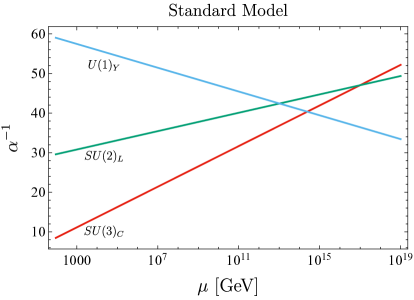
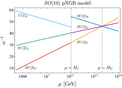
Figure 1: The gauge coupling constants $\alpha_{i}$ vs the energy scale $\mu$ for the SM (the left figure) and the $SO(10)$ pNGB model (the right figure) are shown. The left figure shows the energy dependence of three gauge coupling constants of $SU(3)_{C}$, $SU(2)_{L}$, and $U(1)_{Y}$, $\alpha_{3C}$, $\alpha_{2L}$, and $\alpha_{1Y}$ in all the energy ranges $\mu=[M_{Z},M_{H}]$, where $M_{H}=10^{19}$ GeV. The right figure shows $\alpha_{3C}$, $\alpha_{2L}$, and $\alpha_{1Y}$ in the energy ranges $\mu=[M_{Z},M_{I}]$; $\alpha_{4C}$, $\alpha_{2L}$, $\alpha_{2R}$ in the energy ranges $\mu=[M_{I},M_{H}]$, where the value of $\alpha_{3C}$ is fixed as the central value $\alpha_{3C}(M_{Z})=0.1181$ [53].

As the same as the usual GUT models, nucleon can decay via the so-called lepto-quark gauge bosons. The proton lifetime via the gauge bosons is roughly estimated as $\tau\simeq{M_{U}^{4}}/{\alpha_{U}^{2}m_{p}^{5}}$ [57, 54, 53], where $m_{p}$ is the proton mass and the gauge boson masses are assumed to be $M_{U}$. From the values of $M_{U}$ and $\alpha_{U}$ given in Eqs. (3.23) and (3.26), the proton lifetime $\tau\simeq 1.1\times 10^{37}$ years is predicted. It is far from the current constraint $\tau(p\to e^{+}\pi^{0})>2.4\times 10^{34}$ years at $90\%$ CL [58]; $M_{U}>(4.3-4.8)\times 10^{15}$ GeV for $40\lesssim\alpha_{U}^{-1}\lesssim 50$. There is contribution for the proton decay modes via colored scalar fields shown in Table 3. The color triplet component of $\Phi_{\bf 10}$ has assumed to have $\mathcal{O}(M_{U})$, so the contribution for the proton decay via the Yukawa coupling constant $\mathsf{y}_{\bf 10}^{(ab)}$ of the term $\mathsf{\Phi}_{{\bf 10}}\left(\mathsf{\Psi}_{\bf 16}^{(a)}\mathsf{\Psi}_{\bf 16}^{(b)}\right)_{\bf 10}$ in Eq. (2.1) is small. Color non-singlet components of $\mathsf{\Phi}_{\bf\overline{126}}$ have assumed to $\mathcal{O}(M_{I})$, so the contribution for the proton decay via the Yukawa coupling constant $\mathsf{y}_{\bf\overline{126}}^{(ab)}$ of the term $\mathsf{\Phi}_{\overline{\bf 126}}^{*}\left(\mathsf{\Psi}_{\bf 16}^{(a)}\mathsf{\Psi}_{\bf 16}^{(b)}\right)_{\bf\overline{126}}$ in Eq. (2.1) can be larger than the current experimental bounds. This leads to an upper bound of the values of $\mathsf{y}_{\bf\overline{126}}^{(ab)}$ in the model.

We comment on proton decay via a colored Higgs scalar or lepto-quark scalar denoted as $S_{1}$ in Ref. [59], which belongs to $({\bf 3,1},1/3)$ under $G_{\rm SM}$. In the following, we omit Clebsch-Gordan coefficients for simplicity. When the lepto-quark scalar $S_{1}$ has di-quark and quark-lepton couplings, there are proton decay modes such as $p\to e^{+}\pi^{0}$, and the proton lifetime is roughly estimated as $\tau\simeq m_{LQ}^{4}/(|y|^{2}|z|^{2}m_{p}^{5})$, where $m_{LQ}$ is a lepto-quark mass, $y$ and $z$ represent generic values of relevant Yukawa coupling constants of the lepto-quark with the quark-lepton and quark-quark pairs, respectively. For example, for the lepto-quark with the intermediate scale mass $m_{LQ}=M_{I}$ and the universal Yukawa coupling constants $|y|=|z|$, we obtain a constraint for the Yukawa coupling constants $|y|=|z|\lesssim 4.2\times 10^{-6}$ from the current constraint $\tau(p\to e^{+}\pi^{0})>2.4\times 10^{34}$ years at $90\%$ CL. To apply this for the current model, for the scalar field $S_{1}$ in ${\bf 10}$ of $SO(10)$, which belongs to ${\bf(6,1,1)}$ under $G_{\rm PS}$, the mass of the lepto-quark scalar is the unification scale mass $m_{LQ}=M_{U}$ and the Yukawa coupling constants are roughly expected as $|y|=|z|\simeq|y_{\bf 10}^{(11)}|$. The current constraint $\tau(p\to e^{+}\pi^{0})>2.4\times 10^{34}$ years at $90\%$ CL leads to $|y_{\bf 10}^{(11)}|\lesssim 0.68$. To realize the mass of up quark, $y_{\bf 10}^{(11)}$ is roughly $\mathcal{O}(10^{-5})$, so it is consistent with the current constraint, where the actual values of the Yukawa coupling constants depend on how to realized the observed quark and lepton masses. Next, for the scalar fields $S_{1{\bf(\overline{10},1,3)}}$ and $S_{1{\bf(1,1,3)}}$ in ${\bf\overline{126}}$ of $SO(10)$, which belongs to ${\bf(\overline{10},1,3)}$ and ${\bf(6,1,1)}$ under $G_{\rm PS}$. The lepto-quark scalar $S_{1{\bf(\overline{10},1,3)}}$ and $S_{1{\bf(6,1,1)}}$ have the intermediate scale mass $M_{I}$ and the unification scale mass $M_{U}$, respectively. For $S_{1{\bf(\overline{10},1,3)}}$, the Yukawa coupling couplings are given by $|y|=0$ and $|z|\simeq|y_{\bf\overline{126}}|$, so the proton decay mediated by $S_{1{\bf(\overline{10},1,3)}}$ does not occur. Therefore, this does not lead to any constraint for $y_{\bf\overline{126}}^{(ab)}$. For $S_{1{\bf(6,1,1)}}$, the Yukawa coupling couplings are given by $|y|=|z|\simeq|y_{\bf\overline{126}}|$. the current constraint $\tau(p\to e^{+}\pi^{0})>2.4\times 10^{34}$ years at $90\%$ CL leads to $|y_{\bf\overline{126}}^{(11)}|\lesssim 0.68$ as the same as $S_{1}$ in ${\bf 10}$ of $SO(10)$. In the above discussion, we assumed $S_{1{\bf(\overline{10},1,3)}}$ does not mix with $S_{1{\bf(6,1,1)}}$, but they have the same quantum numbers, so it depends on the structure of the scalar potential, they can be mixed in general. Even when the mixing parameter denoted as $\varepsilon$ between $S_{1{\bf(\overline{10},1,3)}}$ and $S_{1{\bf(6,1,1)}}$ is about the ratio of the masses $\varepsilon\simeq M_{I}/M_{U}\simeq 6.1\times 10^{-6}$, the current constraint $\tau(p\to e^{+}\pi^{0})>2.4\times 10^{34}$ years at $90\%$ CL leads to the constraint for the first generation Yukawa coupling constant $|y_{\bf\overline{126}}^{(11)}|\lesssim 1.7\times 10^{-3}$. (For $\varepsilon=1$, $|y_{\bf\overline{126}}^{(11)}|\lesssim 4.2\times 10^{-6}$.)

Further, we comment on the relation between neutrino masses and the Yukawa coupling constants $y_{\bf\overline{126}}^{(ab)}$ of the cubic term $\mathsf{\Phi}_{\bf 16}\mathsf{\Phi}_{\bf 16}\mathsf{\Phi}_{\bf\overline{126}}$. Since the right-handed neutrino masses are given by $M_{N}^{(ab)}=y_{\bf\overline{126}}^{(ab)}v_{\phi}$, we obtain $2.1\times 10^{8}\,\mbox{GeV}\lesssim M_{N}^{(11)}=y_{\bf\overline{126}}^{(11)}v_{\phi}\lesssim 1.4\times 10^{11}\,\mbox{GeV}$ for $1.7\times 10^{-3}\lesssim y_{\bf\overline{126}}^{(11)}\lesssim 0.68$ and $v_{\phi}=M_{I}$. From the Type-I see-saw mechanism, the light neutrino mass is roughly $m_{\nu}^{(11)}\simeq|y_{\bf 10}^{(11)}v|^{2}/M_{N}^{(11)}$ when we ignore the off-diagonal part of $M_{N}^{(ab)}$. Therefore, $4.4\times 10^{-8}\,\mbox{eV}\lesssim m_{\nu}^{(11)}\lesssim 2.9\times 10^{-5}\,\mbox{eV}$ for $1.7\times 10^{-3}\lesssim y_{\bf\overline{126}}^{(11)}\lesssim 0.68$, $|y_{\bf 10}^{(11)}|\simeq 10^{-5}$ and $v\simeq 246\,\mbox{GeV}$. The proton decay constraints only a part of the Yukawa coupling constants $y_{\bf\overline{126}}^{(ab)}$, so it is expected that the observed neutrino masses can be reproduced, but to perform it properly, we need to investigate how to reproduce the observed quark and charged lepton masses. We leave it for a future study.

Up to this point, we only consider the specific symmetry breaking pattern, $SO(10)$ broken to $G_{I}=G_{\rm PS}$ at $\mu=M_{U}$ in Eq.(1.2). We comment on other cases $G_{I}=G_{\rm PS}\times D$, $G_{\rm LR}$, $G_{\rm LR}\times D$ discussed in e.g., Refs. [55, 56, 60, 41], where $D$ stands for a discrete $Z_{2}$ left-right exchange symmetry [61, 62]. (Note that the same analysis in $SO(10)$ GUT models whose matter content is slightly different from the present model has been already discussed in e.g., Refs. [55, 56] by using two-loop RGEs [63] and the corresponding matching condition [64, 65].) To realize the appropriate symmetry breaking patterns, we need different $SO(10)$ breaking Higgs fields; each $G_{I}=G_{\rm PS}$, $G_{\rm PS}\times D$, $G_{\rm LR}$, $G_{\rm LR}\times D$ is realized by the VEV of a scalar field in e.g., ${\bf 210}$, ${\bf 54}$, ${\bf 45}$, ${\bf 210}$ of $SO(10)$, respectively.

The values of $M_{I}$, $M_{U}$, and $\alpha_{U}^{-1}$ for several matter contents and symmetry breaking patterns are summarized in Table 5, which are estimated by using each analytical solution shown in Appendix B. Substituting the values of $M_{U}$ and $\alpha_{U}^{-1}$ for the $G_{\rm PS}\times D$ and $G_{\rm LR}\times D$ cases into $\tau\simeq{M_{U}^{4}}/{\alpha_{U}^{2}m_{p}^{5}}$, rapid proton decay is expected. For the $G_{\rm LR}$ case, the proton decay via lept-quark gauge bosons is consistent with the current experimental constraints, but the pNGB cannot be identified as DM because pNGB decays too rapidly or the observed relic abundance cannot be reproduced.

Group $G_{I}$	Scalars at $\mu=M_{I}$	$b_{j}$	$\mbox{log}_{10}(M/1\mbox{[GeV]})$ $M_{I}$ $M_{U}$		$\alpha_{U}^{-1}$
$G_{\rm PS}$	$({\bf 1,2,2})_{\bf 10}$ $({\bf\overline{4},1,2})_{\bf 16}$ $({\bf\overline{10},1,3})_{\bf\overline{126}}$	$\left(\begin{array}[]{c}b_{4C}\\ b_{2L}^{\prime}\\ b_{2R}\\ \end{array}\right)=\left(\begin{array}[]{c}-\frac{22}{3}\\ -3\\ +\frac{13}{3}\\ \end{array}\right)$	$11.10\pm 0.08$	$16.31\pm 0.15$	$45.92\pm 0.50$
$G_{\rm PS}\times D$	$({\bf 1,2,2})_{\bf 10}$ $({\bf{4},2,1})_{\bf 16}$ $({\bf\overline{4},1,2})_{\bf 16}$ $({\bf\overline{10},1,3})_{\bf\overline{126}}$ $({\bf 10,3,1})_{\bf\overline{126}}$	$\left(\begin{array}[]{c}b_{4C}\\ b_{2L}^{\prime}\\ b_{2R}\\ \end{array}\right)=\left(\begin{array}[]{c}-4\\ +\frac{13}{3}\\ +\frac{13}{3}\\ \end{array}\right)$	$13.71\pm 0.03$	$15.22\pm 0.04$	$40.82\pm 0.13$
$G_{\rm LR}$	$({\bf 1,2,2},0)_{\bf 10}$ $({\bf 1,1,2},1)_{\bf 16}$ $({\bf 1,1,3},2)_{\bf\overline{126}}$	$\left(\begin{array}[]{c}b_{3C}^{\prime}\\ b_{2L}^{\prime}\\ b_{2R}\\ b_{B-L}\\ \end{array}\right)=\left(\begin{array}[]{c}-7\\ -3\\ -\frac{13}{6}\\ +\frac{23}{4}\\ \end{array}\right)$	$8.57\pm 0.06$	$16.64\pm 0.13$	$46.13\pm 0.41$
$G_{\rm LR}\times D$	$({\bf 1,2,2},0)_{\bf 10}$ $({\bf 1,1,2},1)_{\bf 16}$ $({\bf 1,2,1},1)_{\bf 16}$ $({\bf 1,1,3},2)_{\bf\overline{126}}$ $({\bf 1,3,1},-2)_{\bf\overline{126}}$	$\left(\begin{array}[]{c}b_{3C}^{\prime}\\ b_{2L}^{\prime}\\ b_{2R}\\ b_{B-L}\\ \end{array}\right)=\left(\begin{array}[]{c}-7\\ -\frac{13}{6}\\ -\frac{13}{6}\\ +\frac{15}{2}\\ \end{array}\right)$	$10.11\pm 0.04$	$15.57\pm 0.09$	$43.38\pm 0.30$

Table 5: The values of $M_{I}$, $M_{U}$, and $\alpha_{U}^{-1}$ for several matter contents and symmetry breaking patterns are summarized. The top of the table corresponds to the present $SO(10)$ pNGB model. The first, second, and third columns represent the intermediate scale group $G_{I}$, the matter content for scalar sector at $\mu=M_{I}$, the beta function coefficients $b_{j}$ of $G_{I}$, respectively. The fourth and fifth columns show the values of $M_{I}$, $M_{U}$, and $\alpha_{U}^{-1}$. The subscript in the second column stands for each $SO(10)$ representation.

4 Long-lived pNGB as DM candidate

The DM lifetime should be longer than the age of the universe, $10^{17}\,\mathrm{s}$ at least. The bound on DM lifetime becomes stronger depending on DM decay channels due to the constraint of cosmic-ray observations. In particular, the bound from gamma-ray observations is strong as roughly $\tau_{\chi}\gtrsim 10^{27}\,\mathrm{s}$ for two body decays [66]. Since the DM lifetime is proportional to the power of the VEV $v_{\phi}$, it becomes longer for larger $v_{\phi}$. The evaluation of DM lifetime without GUT has been studied in Refs. [19, 20], and it has turned out that the VEV should roughly be $v_{\phi}\gtrsim 10^{13}\,\mathrm{GeV}$ in order to be consistent with the gamma-ray observations if three body decays $\chi\to h_{i}f\overline{f}$ and $Zf\overline{f}$ can occur. Since in the current GUT pNGB model the kinetic mixing $\sin\epsilon$ and the VEV $v_{\phi}$ are fixed to be $\sin\epsilon=-\sqrt{2/5}$ and $v_{\phi}\simeq 10^{11}\,\mathrm{GeV}$ by the requirement of the gauge coupling unification, the three body decays should kinematically be forbidden. Therefore we consider the mass region $m_{\chi}\lesssim\mathcal{O}(100)\,\mathrm{GeV}$ and estimate dominant four body decay channels.

Before proceeding to four body decays, we comment on the two body decay channel $\chi\to\nu\nu$, which is possible even in the case $m_{\chi}\lesssim\mathcal{O}(100)\,\mathrm{GeV}$. Similarly to the $U(1)_{B-L}$ model in the previous paper [19], this process occurs via the scalar mixing given by Eq. (2.39) and the mixing between the left-handed and right-handed neutrinos after the electroweak symmetry breaking. The decay width for this channel is calculated as

$$\Gamma_{\nu\nu} =\frac{m_{\chi}}{64\pi}\frac{v_{s}^{2}}{v_{\phi}^{4}}\sum_{i}m_{\nu_{i}}^{2}$$

$$=5\times 10^{-59}\,\mathrm{GeV}\left(\frac{m_{\chi}}{100\,\mathrm{GeV}}\right)\left(\frac{v_{s}}{1\,\mathrm{TeV}}\right)^{2}\left(\frac{10^{11}\,\mathrm{GeV}}{v_{\phi}}\right)^{4}\sum_{i}\left(\frac{m_{\nu_{i}}}{0.1\,\mathrm{eV}}\right)^{2},$$ (4.1)

where $m_{\nu_{i}}$ is the small neutrino mass eigenvalues. Eq. (4.1) roughly corresponds to the lifetime $\tau_{\nu\nu}=\mathcal{O}(10^{34})\,\mathrm{s}$, which is too small to be observed in neutrino cosmic-rays [67, 68] because of the suppression by the small neutrino mass squared $m_{\nu_{i}}^{2}$. Note that since the scale of the VEV in the GUT pNGB model is $v_{\phi}\simeq 10^{11}\,\mathrm{GeV}$ which is much smaller than the previous analysis [19], the order of the lifetime for this channel is much shorter. However it is still too long to be detectable by experiments and observations.

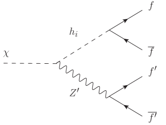
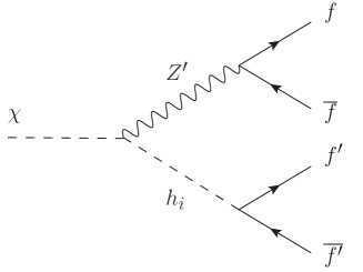
Figure 2: The Feynman diagrams for the four body decays $\chi\to f\bar{f}f^{\prime}\bar{f^{\prime}}$ are shown.

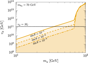
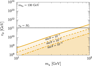
Figure 3: Parameter space in the ($m_{\chi}$, $v_{\phi}$) plane where the second Higgs mass is fixed to be $m_{h_{2}}=70\,\mathrm{GeV}$ in the left and $130\,\mathrm{GeV}$ in the right. The orange region is excluded by the bound of the gamma-ray observations ($\tau_{\chi}=10^{27}\,\mathrm{s}$) for $\sin\theta=10^{-1},10^{-2}$ and $10^{-3}$.

The four body decay processes $\chi\to f\overline{f}f^{\prime}\overline{f^{\prime}}$ mediated by $h_{i},Z,Z^{\prime}$ can occur as shown in Fig. 2. Note that if $f$ and $f^{\prime}$ are identical particles, additional diagrams exist due to interference. We numerically evaluated the decay width for all the four body decay processes using CalcHEP [69], and furthermore we took into account three body decay processes when these are kinematically possible. The results are shown in Fig. 3 in ($m_{\chi}$, $v_{\phi}$) plane where the second Higgs mass is fixed to be $m_{h_{2}}=70\,\mathrm{GeV}$ (left) and $130\,\mathrm{GeV}$ (right). The orange region below the solid, dashed and dot-dashed lines are the region where the DM lifetime is shorter than the conservative bound $\tau_{\chi}=10^{27}\,\mathrm{s}$ for the Higgs mixing angle $\sin\theta=10^{-1},10^{-2},10^{-3}$, respectively. The horizontal black dotted line denotes $v_{\phi}=M_{I}=10^{11.10}\,\mathrm{GeV}$. The most part of the region in the plots is dominated by the four body decays except for the region $m_{\chi}\gtrsim 60\,\mathrm{GeV}$ in the left panel where the three body decay $\chi\to h_{2}f\overline{f}$ can open up. One can read off the upper bound of the DM mass $m_{\chi}$ for a given mixing angle $\sin\theta$.

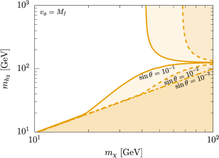
Figure 4: Parameter space in ($m_{\chi}$, $h_{h_{2}}$) plane, where the VEV is fixed to be $v_{\phi}=M_{I}$. The orange region is excluded by the bound of the gamma-ray observations ($\tau_{\chi}=10^{27}\,\mathrm{s}$) for $\sin\theta=10^{-1},10^{-2}$ and $10^{-3}$.

Fig. 4 shows the parameter space in ($m_{\chi}$, $m_{h_{2}}$) plane for the Higgs mixing angle $\sin\theta=10^{-1},10^{-2}$ and $10^{-3}$ where $v_{\phi}=M_{I}$. The region $m_{\chi}\gtrsim m_{h_{2}}$ is strongly constrained by three body decay $\chi\to h_{2}f\overline{f}$ while the other region is constrained by four body decays. In particular, if the second Higgs mass is degenerate with the SM-like Higgs boson ($m_{h_{1}}\simeq m_{h_{2}}$), the four body decay width can be small and the constraint is weaken. This is because the effective coupling $\chi$-$f$-$f^{\prime}$ mediated by $h_{1}$ and $h_{2}$ becomes small when $m_{h_{1}}\simeq m_{h_{2}}$.

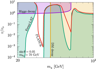
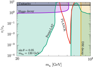
Figure 5: Parameter space thermally reproducing the observed relic abundance consistent with some other observations. The red line represents the parameter space reproducing the correct thermal relic abundance $\Omega_{\chi}h^{2}\simeq 0.12$. The orange and green region are excluded by gamma-ray observations coming from the DM decay and annihilations, respectively. The purple region are excluded by the constraints of the Higgs invisible decay $h_{1}\to\chi\chi$ and the Higgs signal strength. The gray region is perturbative unitarity bound $\lambda_{S}>8\pi/3$.

Thermal relic abundance of DM is calculated using micrOMEGAs [70]. The results are shown in Fig. 5, where the other parameters are fixed to be $m_{h_{2}}=70\,\mathrm{GeV}$, $\sin\theta=0.05$ in the left panel and $m_{h_{2}}=130\,\mathrm{GeV}$ and $\sin\theta=0.05$ the right panel. The red line denotes the parameter space which can reproduce the observed relic abundance of DM $\Omega_{\chi}h^{2}\simeq 0.12$ [4]. The purple region is excluded by the constraints of the Higgs invisible decay and Higgs signal strength [71, 72], and the gray region is excluded by the perturbative unitarity bound $\lambda_{S}<8\pi/3$ [73]. The green and orange region are ruled out by the constraints of the gamma-ray observations for DM annihilations [74] and four body decays [66], respectively. One can see that the thermal relic abundance can be consistent with all the constraints when the DM mass is rather close to the resonances $m_{\chi}\lesssim m_{h_{i}}/2$. This is the characteristic due to the requirement from the gauge coupling unification in the current GUT pNGB model.

We comment on the allowed parameter space $m_{\chi}\lesssim m_{h_{i}}/2$. For the second Higgs mass rather heavier than the SM-like Higgs mass, the constraint of the gamma-ray observations can be avoided only if the DM mass is light enough $m_{\chi}\lesssim 35\,\mathrm{GeV}$ as can be seen from Fig. 4. On the other hand, this mass region cannot be consistent with the thermal relic abundance of DM since it is far from the Higgs resonances. Therefore the mass region $m_{h_{2}}\gtrsim m_{h_{1}}$ is completely excluded as long as thermal production mechanism of DM is assumed. For more precise calculations in the region $m_{\chi}\lesssim m_{h_{i}}/2$, the effect of the early kinetic decoupling from the SM thermal bath should be taken into account [75, 76]. If this effect is included, one can expect that the red line in Fig. 3 is shifted slightly upward.

5 Summary

In this paper, we proposed an $SO(10)$ pNGB DM model in the framework of GUTs. Each Weyl fermion in ${\bf 16}$ of $SO(10)$ contains one generation of quark and leptons. The SM Higgs and two complex scalar fields $H$, $S$ and $\Phi$ in the previous gauged $U(1)_{B-L}$ pNGB DM model are embedded into scalar fields in ${\bf 10}$, ${\bf 16}$, and ${\bf\overline{126}}$ of $SO(10)$. Assuming a symmetry breaking pattern of $SO(10)$ to $G_{\rm PS}$ at $\mu=M_{U}$, and further to $G_{\rm SM}$ at $\mu=M_{I}$, the intermediate and unified scales $M_{I}$ and $M_{U}$, the gauge coupling constants of $U(1)_{B-L}$, and the kinetic mixing parameter of between $U(1)_{Y}$ and $U(1)_{B-L}$ are determined by solving the RGEs with appropriate matching conditions such as gauge coupling unification at $\mu=M_{U}$.

The DM lifetime without GUT has analyzed in Refs. [19, 20]. It suggests that the VEV should roughly be the VEV of $\Phi$ $v_{\phi}\gtrsim 10^{13}\,\mathrm{GeV}$ in order to be consistent with the gamma-ray observations if three body decays $\chi\to h_{i}f\overline{f}$ and $Zf\overline{f}$ are possible. In the current GUT pNGB model, the kinetic mixing and the VEV are fixed to be $\sin\epsilon=-\sqrt{2/5}$ and $v_{\phi}\simeq 10^{11}\,\mathrm{GeV}$, respectively. To satisfy the constraint from the gamma-ray observations, the pNGB DM mass must be $m_{\chi}\lesssim\mathcal{O}(100)\,\mathrm{GeV}$ to forbid the three body decays kinematically. In the mass region, the dominant contribution for DM decay channels comes from four body decay channels $\chi\to f\bar{f}f^{\prime}\bar{f^{\prime}}$. We find that the thermal relic abundance can be consistent with all the constraints when the DM mass is rather close to the resonances $m_{\chi}\lesssim m_{h_{i}}/2$.

Appendix A Kinetic mixing as mass mixing

As discussed in the main part of this paper, the gauge kinetic mixing in Refs. [19, 20] is regarded as the mixing angle. In this appendix, we will show this explicitly. The scalar fields in Refs. [19, 20] are embedded into the scalars of $SO(10)$ shown in Table 3 as

$$\mathsf{\Phi}_{\bm{10}}\supset\phi_{(\bm{1},\bm{2},\bm{2})}\supset\phi_{(\bm{1},\bm{2},1/2)}=H,$$ (A.1)

$$\mathsf{\Phi}_{\bm{16}}\supset\phi_{(\overline{\bm{4}},\bm{1},\bm{2})}\supset\phi_{(\bm{1}(+3),\bm{1},-1/2)}=S,$$ (A.2)

$$\mathsf{\Phi}_{\overline{\bm{126}}}\supset\phi_{(\overline{\bm{10}},\bm{1},\bm{3})}\supset\phi_{(\bm{1}(+6),\bm{1},-1)}=\Phi.$$ (A.3)

Here we will consider the following two symmetry breaking pattern:

$$G_{\mathrm{PS}}\to G_{\mathrm{SM}},\quad G_{\mathrm{PS}}\to G_{\mathrm{LR}}\to G_{\mathrm{SM}}.$$ (A.4)

A.1 $G_{\mathrm{PS}}\to G_{\mathrm{SM}}$

First, let us consider the following symmetry breaking pattern

$$SU(4)_{C}\times SU(2)_{R}\xrightarrow[]{\hskip 2.84526pt\braket{\phi_{(\overline{\bm{10}},\bm{1},\bm{3})}}\neq 0,~{}\braket{\phi_{(\overline{\bm{4}},\bm{1},\bm{2})}}\neq 0\hskip 2.84526pt}SU(3)_{C}\times U(1)_{Y},$$ (A.5)

using minimal scalar fields Eqs. (A.1)–(A.3). This breaking pattern is suitable for the pNGB dark matter model embedding into an $SO(10)$ GUT model because the intermediate scale can be large enough to make the dark matter candidate long-lived.

The covariant derivative of $G_{\mathrm{PS}}$ gauge group acts on $S$ and $\Phi$ as

$$D_{\mu}S =\partial_{\mu}S+ig_{4}G^{\prime\overline{\bm{3}},a}_{\mu}I^{SU(4)_{C}}_{\overline{\bm{3}}(-4),a}S+ig_{B-L}E_{\mu}Q^{S}_{B-L}S+i\frac{g_{R}}{\sqrt{2}}W^{\prime+}_{\mu}I^{SU(2)_{R}}_{+}S+ig_{R}W^{\prime 3}_{\mu}I^{SU(2)_{R}}_{3}S$$

$$=\partial_{\mu}S+ig_{4}G^{\prime\overline{\bm{3}},a}_{\mu}I^{SU(4)_{C}}_{\overline{\bm{3}}(-4),a}S+i\frac{g_{R}}{\sqrt{2}}W^{\prime+}_{\mu}I^{SU(2)_{R}}_{+}S+ig_{B-L}E_{\mu}S-\frac{ig_{R}}{2}W^{\prime 3}_{\mu}S,$$ (A.6)

$$D_{\mu}\Phi =\partial_{\mu}\Phi+ig_{4}G^{\prime\bm{3},a}_{\mu}I^{SU(4)_{C}}_{\bm{3}(4),a}\Phi+ig_{B-L}E_{\mu}Q^{\Phi}_{B-L}\Phi+i\frac{g_{R}}{\sqrt{2}}W^{\prime+}_{\mu}I^{SU(2)_{R}}_{+}\Phi+ig_{R}W^{\prime 3}_{\mu}I^{SU(2)_{R}}_{3}\Phi$$

$$=\partial_{\mu}\Phi+ig_{4}G^{\prime\bm{3},a}_{\mu}I^{SU(4)_{C}}_{\bm{3}(4),a}\Phi+i\frac{g_{R}}{\sqrt{2}}W^{\prime+}_{\mu}I^{SU(2)_{R}}_{+}\Phi+2ig_{B-L}E_{\mu}\Phi-ig_{R}W^{\prime 3}_{\mu}\Phi,$$ (A.7)

where $E_{\mu}$ is the gauge field associated with $U(1)_{B-L}\subset SU(4)_{C}$ and $g_{B-L}$ is the gauge coupling constant given by $g_{B-L}=\sqrt{\frac{3}{8}}g_{4}$. The $B-L$ charge comes from the diagonal component of $SU(4)$ denoted by

$$Q_{B-L}=\sqrt{\frac{8}{3}}I^{SU(4)_{C}}_{15},\quad I^{SU(4)_{C}}_{15}=\sqrt{\frac{3}{8}}\mathop{\mathrm{diag}}(1/3,1/3,1/3,-1).$$ (A.8)

$G^{\prime\bm{3},a}_{\mu}$ and $G^{\prime\overline{\bm{3}},a}_{\mu}$ are color charged vector boson with the representation $\bm{3}(4)$ and $\overline{\bm{3}}(-4)$ of $SU(3)_{C}\times U(1)_{B-L}$ belonging to $\bm{15}$ of $SU(4)_{C}$ respectively. (For the details of the branching rules and the tensor products, see Ref. [30].) These scalars are assumed to develop the following VEVs,

$$\braket{S}=\frac{v_{s}}{\sqrt{2}},\quad\braket{\Phi}=\frac{v_{\phi}}{\sqrt{2}},$$ (A.9)

and these gives the mass terms of the gauge fields

$$\mathcal{L}_{SU(4)_{C}\times SU(2)_{R},\text{mass}}= G^{\prime\bm{3},a\dagger}_{\mu}M^{2}_{\bm{3},ab}G^{\prime\bm{3},b\mu}+G^{\prime\overline{\bm{3}},a\dagger}_{\mu}M^{2}_{\overline{\bm{3}},ab}G^{\prime\overline{\bm{3}},b\mu}+\frac{g_{R}^{2}}{4}(v_{s}^{2}+2v_{\phi}^{2})W^{\prime-}_{\mu}W^{\prime+\mu}$$

$$~{}+\frac{1}{2}\biggl{(}\frac{v_{s}^{2}}{4}+v_{\phi}^{2}\biggr{)}\bigl{(}2g_{B-L}E_{\mu}-g_{R}W^{\prime 3}_{\mu}\bigr{)}^{2},$$ (A.10)

where the mass matrices for the color charged vector bosons $G^{\prime\bm{3},a}_{\mu}$ and $G^{\prime\overline{\bm{3}},a}_{\mu}$ are defined by

$$M^{2}_{\bm{3},ab}=\frac{g_{4}^{2}v_{\phi}^{2}}{2}\mathop{\mathrm{tr}}\nolimits\Bigl{[}\bigl{(}I^{SU(4)_{C}}_{\bm{3}(4),a}\bigr{)}^{\dagger}I^{SU(4)_{C}}_{\bm{3}(4),b}\Bigr{]},\quad M^{2}_{\overline{\bm{3}},ab}=\frac{g_{4}^{2}v_{s}^{2}}{2}\mathop{\mathrm{tr}}\nolimits\Bigl{[}\bigl{(}I^{SU(4)_{C}}_{\overline{\bm{3}}(-4),a}\bigr{)}^{\dagger}I^{SU(4)_{C}}_{\overline{\bm{3}}(-4),b}\Bigr{]}.$$ (A.11)

The last term of Eq. (A.10) leads the mass mixing between $U(1)_{B-L}\subset SU(4)_{C}$ and $U(1)_{R}\subset SU(2)_{R}$, and the massless direction becomes $U(1)_{Y}$ in the SM gauge group. From this term, the massive vector boson $C^{\prime}_{\mu}$ and the orthogonal massless gauge boson $B^{\prime}_{\mu}$ are introduced by

$$\begin{pmatrix}B^{\prime}_{\mu}\\ C^{\prime}_{\mu}\end{pmatrix}=\begin{pmatrix}\cos\epsilon&\sin\epsilon\\ -\sin\epsilon&\cos\epsilon\end{pmatrix}\begin{pmatrix}W^{\prime 3}_{\mu}\\ E_{\mu}\end{pmatrix},$$ (A.12)

where the mixing angle is defined by

$$\sin\epsilon=\frac{g_{R}}{\sqrt{g_{R}^{2}+4g_{B-L}^{2}}},\quad\cos\epsilon=\frac{2g_{B-L}}{\sqrt{g_{R}^{2}+4g_{B-L}^{2}}},$$ (A.13)

and the mass of $C^{\prime}_{\mu}$ becomes $M_{C^{\prime}}^{2}=(g_{R}^{2}+4g_{B-L}^{2})(v_{s}^{2}/4+v_{\phi}^{2})$. In this basis, the Lagrangian is

$$\mathcal{L}\supset-\frac{1}{4}W^{a}_{\mu\nu}W^{a\mu\nu}-\frac{1}{4}B_{\mu\nu}^{\prime}B^{\prime\mu\nu}-\frac{1}{4}C_{\mu\nu}^{\prime}C^{\prime\mu\nu}+\frac{1}{2}M_{C^{\prime}}^{2}C_{\mu}^{\prime}C^{\prime\mu}$$ (A.14)

If the color charged vector bosons are dropped, the covariant derivative is rewritten by using these bosons as

$$D_{\mu}\supset ig_{1}B^{\prime}_{\mu}+ig_{C^{\prime}}C^{\prime}_{\mu}\biggl{(}\frac{Q_{B-L}}{2}-\sin^{2}\epsilon\,Q_{Y}\biggr{)},$$ (A.15)

where the hypercharge is defined by

$$Q_{Y}=I^{SU(2)_{R}}_{3}+\frac{Q_{B-L}}{2},$$ (A.16)

and the couplings are given by

$$g_{1}=\frac{2g_{R}g_{B-L}}{\sqrt{g_{R}^{2}+4g_{B-L}^{2}}},\quad g_{C^{\prime}}=\sqrt{g_{R}^{2}+4g_{B-L}^{2}}.$$ (A.17)

Correspondence between the pNGB model [19, 20] and the $SO(10)$ pNGB model

We will discuss the kinetic mixing in the GUT model. First, from Eq. (A.12), $B^{\prime}_{\mu}$ is written by using $(W^{\prime 3}_{\mu},E_{\mu})$ as $B^{\prime}_{\mu}=W^{\prime 3}_{\mu}/\cos\epsilon+\sin\epsilon E_{\mu}/\cos\epsilon$, and the field redefinition by $\cos\epsilon$ leads the canonically normalized gauge kinetic terms. The massive direction of broken $U(1)$ symmetry does not change in this rewriting. Then Let us introduce new fields after the rescaling by

$$\begin{pmatrix}B_{\mu}^{\prime}\\ C_{\mu}^{\prime}\end{pmatrix}=\begin{pmatrix}1&\sin\epsilon\\ 0&\cos\epsilon\end{pmatrix}\begin{pmatrix}B_{\mu}\\ C_{\mu}\end{pmatrix},\quad\begin{pmatrix}B_{\mu}\\ C_{\mu}\end{pmatrix}=\begin{pmatrix}1&-\tan\epsilon\\ 0&1/\cos\epsilon\end{pmatrix}\begin{pmatrix}B_{\mu}^{\prime}\\ C^{\prime}_{\mu}\end{pmatrix},$$ (A.18)

so that the massive direction does not change but the massless component is replaced. The relation between $(W^{\prime 3}_{\mu},E_{\mu})$ and $(B_{\mu},C_{\mu})$ is given by

$$\begin{pmatrix}W^{\prime 3}_{\mu}\\ E_{\mu}\end{pmatrix}=\begin{pmatrix}\cos\epsilon&0\\ \sin\epsilon&1\end{pmatrix}\begin{pmatrix}B_{\mu}\\ C_{\mu}\end{pmatrix}.$$ (A.19)

The $U(1)_{B-L}\times U(1)_{R}$ gauge sector in the Lagrangian (A.14) is rewritten by using these fields as

$$\mathcal{L}\supset-\frac{1}{4}W^{a}_{\mu\nu}W^{a\mu\nu}-\frac{1}{4}B_{\mu\nu}B^{\mu\nu}-\frac{1}{4}C_{\mu\nu}C^{\mu\nu}-\frac{\sin\epsilon}{2}B_{\mu\nu}C^{\mu\nu}+\frac{1}{2}M_{C}^{2}C_{\mu}C^{\mu},$$ (A.20)

with $M_{C}^{2}=g_{B-L}^{2}(v_{s}^{2}+4v_{\phi}^{2})$, and the covariant derivative is given by

$$D_{\mu}\supset ~{}ig_{B-L}E_{\mu}Q_{B-L}+ig_{R}W^{\prime 3}_{\mu}I^{SU(2)_{R}}_{3}=ig_{B-L}C_{\mu}Q_{B-L}+ig_{1}B_{\mu}Q_{Y},$$ (A.21)

where Eqs. (A.16) and (A.17) are used. Eqs. (A.20) and (A.21) are parts of the Lagrangian of the gauged $U(1)_{B-L}$ pNGB model, and the gauge kinetic mixing is naturally regarded as the mixing angle coming from the GUT inspired symmetry breaking. The correspondence is summarized in Table 6.

Gauged $U(1)_{B-L}$ model [19]	pNGB in $SO(10)$ GUT
$G_{\mathrm{SM}}\times U(1)_{B-L}$	$G_{\mathrm{PS}}$
$Q_{Y}$	$Q_{Y}=I_{3}^{SU(2)_{R}}+\frac{Q_{B-L}}{2}$
$Q_{B-L}$	$Q_{B-L}=\sqrt{\frac{8}{3}}I^{SU(4)_{C}}_{15}$
$B_{\mu}$	$B_{\mu}$ in Eq. (A.18)
$\hat{B}_{\mu}$	$B_{\mu}^{\prime}$ in Eq. (A.12)
$X_{\mu}$	$C_{\mu}$ in Eq. (A.18)
$\hat{X}_{\mu}$	$C^{\prime}_{\mu}$ in Eq. (A.12)
$g_{1}$	$g_{1}=2g_{R}g_{B-L}/\sqrt{g_{R}^{2}+4g_{B-L}^{2}}$
$g_{B-L}$	$g_{B-L}=\sqrt{\frac{3}{8}}g_{4}$
$g_{2}$	$g_{L}$
$D_{\mu}=\partial_{\mu}+ig_{s}G^{a}_{\mu}I^{SU(3)_{C}}_{a}+ig_{2}W^{a}_{\mu}I^{SU(2)_{L}}_{a}$	$D_{\mu}=\partial_{\mu}+ig_{s}G^{a}_{\mu}I^{SU(3)_{C}}_{a}+ig_{L}W^{a}_{\mu}I^{SU(2)_{L}}_{a}$
$+ig_{1}Q_{Y}B_{\mu}+ig_{B-L}Q_{B-L}X_{\mu}$	$+ig_{1}Q_{Y}B_{\mu}+ig_{B-L}Q_{B-L}C_{\mu}$
kinetic mixing
gauge kinetic mixing of $B_{\mu}$ and $X_{\mu}$: $\epsilon$	gauge kinetic mixing of $B_{\mu}$ and $C_{\mu}$: $\epsilon$
$=$ free parameter	$=$ mixing angle $\epsilon$ of $(W^{\prime 3}_{\mu},E_{\mu})\mapsto(B^{\prime}_{\mu},C^{\prime}_{\mu})$
	in Eq. (A.14)

Table 6: The correspondence table of the kinetic mixing and the gauge fields between the gauged $U(1)_{B-L}$ model [19, 20] and $SO(10)$ GUT model.

A.2 $G_{\mathrm{PS}}\to G_{\mathrm{LR}}\to G_{\mathrm{SM}}$

If the adjoint Higgs bosons $\phi_{(\bm{15},\bm{1},\bm{1})}$ and $\phi_{(\bm{1},\bm{1},\bm{3})}$ are introduced in addition to the scalars Eqs. (A.1)–(A.3), these VEVs break the Pati-Salam gauge symmetry as

$$SU(4)_{C}\xrightarrow[]{\hskip 2.84526pt\braket{\phi_{(\bm{15},\bm{1},\bm{1})}}\neq 0\hskip 2.84526pt}SU(3)_{C}\times U(1)_{B-L},\quad SU(2)_{R}\xrightarrow[]{\hskip 2.84526pt\braket{\phi_{(\bm{1},\bm{1},\bm{3})}}\neq 0\hskip 2.84526pt}U(1)_{R}.$$ (A.22)

By this breaking pattern, the covariant derivative of $G_{\mathrm{PS}}$ reduces to that of $SU(3)_{C}\times SU(2)_{L}\times U(1)_{R3}\times U(1)_{B-L}$ as

$$D_{\mu}=\partial_{\mu}+ig_{s}G^{a}_{\mu}I^{SU(3)_{C}}_{a}+ig_{B-L}E_{\mu}Q_{B-L}+ig_{L}W^{a}_{\mu}I^{SU(2)_{L}}_{a}+ig_{R}W^{\prime 3}_{\mu}I^{SU(2)_{R}}_{3},$$ (A.23)

where the $B-L$ charge is defined by Eq. (A.8) and the gauge couplings are introduced by $g_{s}=g_{4}$, $g_{C}=\sqrt{\frac{3}{8}}g_{4}$. The VEVs of $S$ and $\phi$ (A.9) break the residual gauge symmetry as

$$SU(3)_{C}\times SU(2)_{L}\times U(1)_{R}\times U(1)_{B-L}\to G_{\mathrm{SM}},$$ (A.24)

and lead the mass term for the gauge bosons

$$\mathcal{L}_{U(1)_{R3}\times U(1)_{B-L},\text{mass}}=\frac{1}{2}\biggl{(}\frac{v_{s}^{2}}{4}+v_{\phi}^{2}\biggr{)}\bigl{(}2g_{B-L}E_{\mu}-g_{R}W^{\prime 3}_{\mu}\bigr{)}^{2},$$ (A.25)

which is same to the last term of Eq. (A.10). In this breaking pattern, the charged gauge bosons become massive via the VEV of the adjoint Higgs fields.

The mixing angle $\epsilon$ and correspondence between the mixing angle and kinetic mixing are same in the previous discussions.

Appendix B RGEs for gauge coupling constants

Here we analyze the RGEs for gauge coupling constants of $G_{\rm SM}$ and $G_{I}=G_{\rm PS},G_{\rm LR}$, and $SO(10)$ in the pNGB DM model. (For the RGE analysis, see e.g., Ref. [54].)

The RGE for the gauge coupling constants given in Eq. (3.1) can be solve as

$$\alpha_{i}^{-1}(\mu_{1})=\alpha_{i}^{-1}(\mu_{0})-\frac{b_{i}}{2\pi}\log\left(\frac{\mu_{1}}{\mu_{0}}\right).$$ (B.1)

when the beta function coefficients $b_{i}$ are constant in the energy range $\mu_{0}<\mu<\mu_{1}$. In the following, we apply the solution for $G_{\rm SM}$, and $G_{I}=G_{\rm PS},G_{\rm LR}$ cases.

In the following, we find the intermediate scale $M_{I}$ and $M_{U}$ can be described by using the gauge coupling constants of $G_{\rm SM}$ at $\mu=M_{Z}$ and the beta function coefficients of $G_{\rm SM}$ and $G_{I}(=G_{\rm PS},G_{\rm LR})$. Therefore, all the gauge coupling constants such as the unified gauge coupling constant $\alpha_{U}$ can be analytically solved if they exist.

B.1 $G_{I}=G_{\rm PS}$ case

We list up the RGEs of $G_{\rm SM}$ and $G_{\rm PS}$ in $M_{Z}<\mu<M_{I}$ and $M_{I}<\mu<M_{U}$, respectively, and the matching conditions at $\mu=M_{I},M_{U}$.

B.1.1 $M_{Z}<\mu<M_{I}$

For $M_{Z}<\mu<M_{I}$, the RGEs of the gauge coupling constants of $G_{\rm SM}=SU(3)_{C}\times SU(2)_{L}\times U(1)_{Y}$ are given by

$$\alpha_{3C}^{-1}(\mu) =\alpha_{3C}^{-1}(M_{Z})-\frac{b_{3C}}{2\pi}\log\left(\frac{\mu}{M_{Z}}\right),\allowdisplaybreaks[1]$$

$$\alpha_{2L}^{-1}(\mu) =\alpha_{2L}^{-1}(M_{Z})-\frac{b_{2L}}{2\pi}\log\left(\frac{\mu}{M_{Z}}\right),\allowdisplaybreaks[1]$$

$$\alpha_{1Y}^{-1}(\mu) =\alpha_{1Y}^{-1}(M_{Z})-\frac{b_{1Y}}{2\pi}\log\left(\frac{\mu}{M_{Z}}\right).$$ (B.2)

B.1.2 $\mu=M_{I}$

The matching conditions between $G_{\rm SM}$ and $G_{\rm PS}=SU(4)_{C}\times SU(2)_{L}\times SU(2)_{R}$ at $\mu=M_{I}$ are given as

$$\alpha_{4C}^{-1}(M_{I}) =\alpha_{3C}^{-1}(M_{I}),\allowdisplaybreaks[1]$$

$$\alpha_{2L}^{\prime-1}(M_{I}) =\alpha_{2L}^{-1}(M_{I}),\allowdisplaybreaks[1]$$

$$\alpha_{2R}^{-1}(M_{I}) =\frac{5}{3}\alpha_{1Y}^{-1}(M_{I})-\frac{2}{3}\alpha_{3C}^{-1}(M_{I}).$$ (B.3)

B.1.3 $M_{I}<\mu<M_{U}$

For $M_{I}<\mu<M_{U}$, the RGEs of the gauge coupling constants of $G_{\rm PS}$ are given by

$$\alpha_{4C}^{-1}(\mu) =\alpha_{4C}^{-1}(M_{I})-\frac{b_{4C}}{2\pi}\log\left(\frac{\mu}{M_{I}}\right)=\alpha_{3C}^{-1}(M_{Z})-\frac{b_{3C}}{2\pi}\log\left(\frac{M_{I}}{M_{Z}}\right)-\frac{b_{4C}}{2\pi}\log\left(\frac{\mu}{M_{I}}\right),\allowdisplaybreaks[1]$$

$$\alpha_{2L}^{\prime-1}(\mu) =\alpha_{2L}^{\prime-1}(M_{I})-\frac{b_{2L}^{\prime}}{2\pi}\log\left(\frac{\mu}{M_{I}}\right)=\alpha_{2L}^{-1}(M_{Z})-\frac{b_{2L}}{2\pi}\log\left(\frac{M_{I}}{M_{Z}}\right)-\frac{b_{2L}^{\prime}}{2\pi}\log\left(\frac{\mu}{M_{I}}\right),\allowdisplaybreaks[1]$$

$$\alpha_{2R}^{-1}(\mu) =\alpha_{2R}^{-1}(M_{I})-\frac{b_{2R}}{2\pi}\log\left(\frac{\mu}{M_{I}}\right)$$

$$=\frac{5}{3}\alpha_{1Y}^{-1}(M_{Z})-\frac{2}{3}\alpha_{3C}^{-1}(M_{Z})-\left(\frac{5}{3}\frac{b_{1Y}}{2\pi}-\frac{2}{3}\frac{b_{3C}}{2\pi}\right)\log\left(\frac{M_{I}}{M_{Z}}\right)-\frac{b_{2R}}{2\pi}\log\left(\frac{\mu}{M_{I}}\right).$$ (B.4)

B.1.4 $\mu=M_{U}$

For $\mu=M_{U}$, the matching condition between $G_{\rm PS}$ and $SO(10)$ at $\mu=M_{U}$ is given by

$$\alpha_{4C}^{-1}(M_{U})=\alpha_{2L}^{\prime-1}(M_{U})=\alpha_{2R}^{-1}(M_{U}),$$ (B.5)

where

$$\alpha_{4C}^{-1}(M_{U}) =\alpha_{3C}^{-1}(M_{Z})-\frac{b_{3C}}{2\pi}\log\left(\frac{M_{I}}{M_{Z}}\right)-\frac{b_{4C}}{2\pi}\log\left(\frac{M_{U}}{M_{I}}\right),\allowdisplaybreaks[1]$$

$$\alpha_{2L}^{\prime-1}(M_{U}) =\alpha_{2L}^{-1}(M_{Z})-\frac{b_{2L}}{2\pi}\log\left(\frac{M_{I}}{M_{Z}}\right)-\frac{b_{2L}^{\prime}}{2\pi}\log\left(\frac{M_{U}}{M_{I}}\right),\allowdisplaybreaks[1]$$

$$\alpha_{2R}^{-1}(M_{U}) =\frac{5}{3}\alpha_{1Y}^{-1}(M_{Z})-\frac{2}{3}\alpha_{3C}^{-1}(M_{Z})-\left(\frac{5}{3}\frac{b_{1Y}}{2\pi}-\frac{2}{3}\frac{b_{3C}}{2\pi}\right)\log\left(\frac{M_{I}}{M_{Z}}\right)-\frac{b_{2R}}{2\pi}\log\left(\frac{M_{U}}{M_{I}}\right).$$ (B.6)

B.1.5 $M_{I}$ and $M_{U}$

From the matching condition in Eq. (B.5), we can analytically solve the intermediate scale $M_{I}$ and unification scale $M_{U}$ as

$$M_{I} =M_{Z}\ \mbox{exp}\left[\frac{A_{1}B_{3}-A_{3}B_{1}}{A_{2}B_{3}-A_{3}B_{2}}\right],$$

$$M_{U} =M_{Z}\ \mbox{exp}\left[\left(\frac{A_{1}B_{3}-A_{3}B_{1}}{A_{2}B_{3}-A_{3}B_{2}}\right)+\left(\frac{A_{1}B_{2}-A_{2}B_{1}}{A_{3}B_{2}-A_{2}B_{3}}\right)\right],$$ (B.7)

where

$$A_{1}=\alpha_{3C}^{-1}(M_{Z})-\alpha_{2L}^{-1}(M_{Z}),\ A_{2}=\frac{b_{3C}-b_{2L}}{2\pi},\ A_{3}=\frac{b_{4C}-b_{2L}^{\prime}}{2\pi},$$

$$B_{1}=\frac{5}{3}\left(\alpha_{3C}^{-1}(M_{Z})-\alpha_{1Y}^{-1}(M_{Z})\right),\ B_{2}=\frac{5}{3}\frac{b_{3C}-b_{1Y}}{2\pi},\ B_{3}=\frac{b_{4C}-b_{2R}}{2\pi}.$$ (B.8)

B.2 $G_{I}=G_{\rm LR}$ case

We list up the RGEs of $G_{\rm SM}$ and $G_{I}=G_{\rm LR}$ in $M_{Z}<\mu<M_{I}$ and $M_{I}<\mu<M_{U}$, respectively, and the matching conditions at $\mu=M_{I},M_{U}$.

B.2.1 $M_{Z}<\mu<M_{I}$

For $M_{Z}<\mu<M_{I}$, the RGEs of the gauge coupling constants of $G_{\rm SM}=SU(3)_{C}\times SU(2)_{L}\times U(1)_{Y}$ are given by

$$\alpha_{3C}^{-1}(\mu) =\alpha_{3C}^{-1}(M_{Z})-\frac{b_{3C}}{2\pi}\log\left(\frac{\mu}{M_{Z}}\right),\allowdisplaybreaks[1]$$

$$\alpha_{2L}^{-1}(\mu) =\alpha_{2L}^{-1}(M_{Z})-\frac{b_{2L}}{2\pi}\log\left(\frac{\mu}{M_{Z}}\right),\allowdisplaybreaks[1]$$

$$\alpha_{1Y}^{-1}(\mu) =\alpha_{1Y}^{-1}(M_{Z})-\frac{b_{1Y}}{2\pi}\log\left(\frac{\mu}{M_{Z}}\right).$$ (B.9)

B.2.2 $\mu=M_{I}$

The matching conditions between $G_{\rm SM}$ and $G_{\rm LR}=SU(3)_{C}\times SU(2)_{L}\times SU(2)_{R}\times U(1)_{B-L}$ at $\mu=M_{I}$ are given as

$$\alpha_{3C}^{\prime-1}(M_{I}) =\alpha_{3C}^{-1}(M_{I}),\allowdisplaybreaks[1]$$

$$\alpha_{2L}^{\prime-1}(M_{I}) =\alpha_{2L}^{-1}(M_{I}),\allowdisplaybreaks[1]$$

$$\alpha_{2R}^{-1}(M_{I}) =\frac{5}{3}\alpha_{1Y}^{-1}(M_{I})-\frac{2}{3}\alpha_{B-L}^{-1}(M_{I}).$$ (B.10)

Note that unlike the above $G_{I}=G_{\rm PS}$ case, the gauge coupling constants of $G_{\rm LR}$ at $\mu=M_{I}$ cannot be determined only by using those of $G_{\rm SM}$ at $\mu=M_{I}$. To fix them, we need to use the matching conditions of the gauge coupling constants at $\mu=M_{U}$.

B.2.3 $M_{I}<\mu<M_{U}$

For $M_{I}<\mu<M_{U}$, the RGEs of the gauge coupling constants of $G_{\rm LR}$ are given by

$$\alpha_{3C}^{\prime-1}(\mu) =\alpha_{3C}^{\prime-1}(M_{I})-\frac{b_{3C}^{\prime}}{2\pi}\log\left(\frac{\mu}{M_{I}}\right)=\alpha_{3C}^{-1}(M_{Z})-\frac{b_{3C}}{2\pi}\log\left(\frac{M_{I}}{M_{Z}}\right)-\frac{b_{3C}^{\prime}}{2\pi}\log\left(\frac{\mu}{M_{I}}\right),\allowdisplaybreaks[1]$$

$$\alpha_{2L}^{\prime-1}(\mu) =\alpha_{2L}^{\prime-1}(M_{I})-\frac{b_{2L}^{\prime}}{2\pi}\log\left(\frac{\mu}{M_{I}}\right)=\alpha_{2L}^{-1}(M_{Z})-\frac{b_{2L}}{2\pi}\log\left(\frac{M_{I}}{M_{Z}}\right)-\frac{b_{2L}^{\prime}}{2\pi}\log\left(\frac{\mu}{M_{I}}\right),\allowdisplaybreaks[1]$$

$$\alpha_{2R}^{-1}(\mu) =\alpha_{2R}^{-1}(M_{I})-\frac{b_{2R}}{2\pi}\log\left(\frac{\mu}{M_{I}}\right),\allowdisplaybreaks[1]$$

$$\alpha_{B-L}^{-1}(\mu) =\alpha_{B-L}^{-1}(M_{I})-\frac{b_{B-L}}{2\pi}\log\left(\frac{\mu}{M_{I}}\right).$$ (B.11)

B.2.4 $\mu=M_{U}$

For $\mu=M_{U}$, the matching condition between $G_{\rm LR}$ and $SO(10)$ at $\mu=M_{U}$ is given by

$$\alpha_{3C}^{\prime-1}(M_{U})=\alpha_{2L}^{\prime-1}(M_{U})=\alpha_{2R}^{-1}(M_{U})=\alpha_{B-L}^{-1}(M_{U}),$$ (B.12)

where

$$\alpha_{3C}^{\prime-1}(M_{U}) =\alpha_{3C}^{-1}(M_{Z})-\frac{b_{3C}}{2\pi}\log\left(\frac{M_{I}}{M_{Z}}\right)-\frac{b_{3C}^{\prime}}{2\pi}\log\left(\frac{M_{U}}{M_{I}}\right),\allowdisplaybreaks[1]$$

$$\alpha_{2L}^{\prime-1}(M_{U}) =\alpha_{2L}^{-1}(M_{Z})-\frac{b_{2L}}{2\pi}\log\left(\frac{M_{I}}{M_{Z}}\right)-\frac{b_{2L}^{\prime}}{2\pi}\log\left(\frac{M_{U}}{M_{I}}\right),\allowdisplaybreaks[1]$$

$$\alpha_{2R}^{-1}(M_{U}) =\frac{5}{3}\alpha_{1Y}^{-1}(M_{Z})-\frac{2}{3}\alpha_{B-L}^{-1}(M_{I})-\frac{5}{3}\frac{b_{1Y}}{2\pi}\log\left(\frac{M_{I}}{M_{Z}}\right)-\frac{b_{2R}}{2\pi}\log\left(\frac{M_{U}}{M_{I}}\right),\allowdisplaybreaks[1]$$

$$\alpha_{B-L}^{-1}(M_{U}) =\alpha_{B-L}^{-1}(M_{I})-\frac{b_{B-L}}{2\pi}\log\left(\frac{M_{U}}{M_{I}}\right).$$ (B.13)

B.2.5 $M_{I}$ and $M_{U}$

From the matching condition in Eq. (B.12), we can analytically solve the intermediate scale $M_{I}$ and unification scale $M_{U}$ as

$$M_{I} =M_{Z}\ \mbox{exp}\left[\frac{C_{1}D_{3}-C_{3}D_{1}}{C_{2}D_{3}-C_{3}D_{2}}\right],\allowdisplaybreaks[1]$$

$$M_{U} =M_{Z}\ \mbox{exp}\left[\left(\frac{C_{1}D_{3}-C_{3}D_{1}}{C_{2}D_{3}-C_{3}D_{2}}\right)+\left(\frac{C_{1}D_{2}-C_{2}D_{1}}{C_{3}D_{2}-C_{2}D_{3}}\right)\right],$$ (B.14)

where

$$C_{1}=\alpha_{3C}^{-1}(M_{Z})-\alpha_{2L}^{-1}(M_{Z}),\ C_{2}=\frac{b_{3C}-b_{2L}}{2\pi},\ C_{3}=\frac{b_{3C}^{\prime}-b_{2L}^{\prime}}{2\pi},\allowdisplaybreaks[1]$$

$$D_{1}=\alpha_{2L}^{-1}(M_{Z})-\alpha_{1Y}^{-1}(M_{Z}),\ D_{2}=\frac{b_{2L}-b_{1Y}}{2\pi},\ D_{3}=\frac{b_{2L}^{\prime}-\frac{3b_{2R}+2b_{B-L}}{5}}{2\pi}.$$ (B.15)

References

- [1] E. Corbelli and P. Salucci, “The Extended Rotation Curve and the Dark Matter Halo of M33,” Mon. Not. Roy. Astron. Soc. 311 (2000) 441–447, arXiv:astro-ph/9909252.
- [2] Y. Sofue and V. Rubin, “Rotation Curves of Spiral Galaxies,” Ann. Rev. Astron. Astrophys. 39 (2001) 137–174, arXiv:astro-ph/0010594.
- [3] R. Massey, T. Kitching, and J. Richard, “The Dark Matter of Gravitational Lensing,” Rept. Prog. Phys. 73 (2010) 086901, arXiv:1001.1739 [astro-ph.CO].
- [4] Planck Collaboration, N. Aghanim et al., “Planck 2018 Results. VI. Cosmological Parameters,” Astron. Astrophys. 641 (2020) A6, arXiv:1807.06209 [astro-ph.CO].
- [5] S. W. Randall, M. Markevitch, D. Clowe, A. H. Gonzalez, and M. Bradac, “Constraints on the Self-Interaction Cross-Section of Dark Matter from Numerical Simulations of the Merging Galaxy Cluster 1E 0657-56,” Astrophys. J. 679 (2008) 1173–1180, arXiv:0704.0261 [astro-ph].
- [6] M. Freytsis and Z. Ligeti, “On Dark Matter Models with Uniquely Spin-Dependent Detection Possibilities,” Phys. Rev. D 83 (2011) 115009, arXiv:1012.5317 [hep-ph].
- [7] S. Ipek, D. McKeen, and A. E. Nelson, “A Renormalizable Model for the Galactic Center Gamma Ray Excess from Dark Matter Annihilation,” Phys. Rev. D 90 no. 5, (2014) 055021, arXiv:1404.3716 [hep-ph].
- [8] G. Arcadi, M. Lindner, F. S. Queiroz, W. Rodejohann, and S. Vogl, “Pseudoscalar Mediators: A WIMP Model at the Neutrino Floor,” JCAP 03 (2018) 042, arXiv:1711.02110 [hep-ph].
- [9] N. F. Bell, G. Busoni, and I. W. Sanderson, “Loop Effects in Direct Detection,” JCAP 08 (2018) 017, arXiv:1803.01574 [hep-ph]. [Erratum: JCAP 01, E01 (2019)].
- [10] T. Abe, M. Fujiwara, and J. Hisano, “Loop Corrections to Dark Matter Direct Detection in a Pseudoscalar Mediator Dark Matter Model,” JHEP 02 (2019) 028, arXiv:1810.01039 [hep-ph].
- [11] T. Abe, M. Fujiwara, J. Hisano, and Y. Shoji, “Maximum Value of the Spin-Independent Cross Section in the 2HDM+a,” JHEP 01 (2020) 114, arXiv:1910.09771 [hep-ph].
- [12] V. Barger, M. McCaskey, and G. Shaughnessy, “Complex Scalar Dark Matter vis-a-vis CoGeNT, DAMA/LIBRA and XENON100,” Phys. Rev. D 82 (2010) 035019, arXiv:1005.3328 [hep-ph].
- [13] C. Gross, O. Lebedev, and T. Toma, “Cancellation Mechanism for Dark-Matter–Nucleon Interaction,” Phys. Rev. Lett. 119 no. 19, (2017) 191801, arXiv:1708.02253 [hep-ph].
- [14] K. Ishiwata and T. Toma, “Probing Pseudo Nambu-Goldstone Boson Dark Matter at Loop Level,” JHEP 12 (2018) 089, arXiv:1810.08139 [hep-ph].
- [15] K. Huitu, N. Koivunen, O. Lebedev, S. Mondal, and T. Toma, “Probing Pseudo-Goldstone Dark Matter at the LHC,” Phys. Rev. D 100 no. 1, (2019) 015009, arXiv:1812.05952 [hep-ph].
- [16] J. M. Cline and T. Toma, “Pseudo-Goldstone Dark Matter Confronts Cosmic Ray and Collider Anomalies,” Phys. Rev. D 100 no. 3, (2019) 035023, arXiv:1906.02175 [hep-ph].
- [17] X.-M. Jiang, C. Cai, Z.-H. Yu, Y.-P. Zeng, and H.-H. Zhang, “Pseudo-Nambu-Goldstone Dark Matter and Two-Higgs-Doublet Models,” Phys. Rev. D 100 no. 7, (2019) 075011, arXiv:1907.09684 [hep-ph].
- [18] C. Arina, A. Beniwal, C. Degrande, J. Heisig, and A. Scaffidi, “Global Fit of Pseudo-Nambu-Goldstone Dark Matter,” JHEP 04 (2020) 015, arXiv:1912.04008 [hep-ph].
- [19] Y. Abe, T. Toma, and K. Tsumura, “Pseudo-Nambu-Goldstone Dark Matter from Gauged Symmetry,” JHEP 05 (2020) 057, arXiv:2001.03954 [hep-ph].
- [20] N. Okada, D. Raut, and Q. Shafi, “Pseudo-Goldstone Dark Matter in a Gauged Extended Standard Model,” Phys. Rev. D 103 no. 5, (2021) 055024, arXiv:2001.05910 [hep-ph].
- [21] Z. Zhang, C. Cai, X.-M. Jiang, Y.-L. Tang, Z.-H. Yu, and H.-H. Zhang, “Phase Transition Gravitational Waves from Pseudo-Nambu-Goldstone Dark Matter and Two Higgs Doublets,” JHEP 05 (2021) 160, arXiv:2102.01588 [hep-ph].
- [22] H. Georgi and S. L. Glashow, “Unity of All Elementary Particle Forces,” Phys. Rev. Lett. 32 (1974) 438–441.
- [23] J. Heeck and V. Takhistov, “Inclusive Nucleon Decay Searches as a Frontier of Baryon Number Violation,” Phys. Rev. D 101 no. 1, (2020) 015005, arXiv:1910.07647 [hep-ph].
- [24] P. Minkowski, “ at a Rate of One Out of Muon Decays?,” Phys. Lett. B 67 (1977) 421–428.
- [25] H. Fritzsch and P. Minkowski, “Unified Interactions of Leptons and Hadrons,” Ann. Phys. 93 (1975) 193–266.
- [26] J. C. Pati and A. Salam, “Lepton Number as the Fourth Color,” Phys. Rev. D10 (1974) 275–289.
- [27] J. Pati, A. Salam, and J. Strathdee, “On Fermion number and its conservation,” Nuovo Cim. A 26 (1975) 72–83.
- [28] R. N. Mohapatra and G. Senjanovic, “Natural Suppression of Strong P and T Noninvariance,” Phys. Lett. B79 (1978) 283–286.
- [29] R. Slansky, “Group Theory for Unified Model Building,” Phys. Rept. 79 (1981) 1–128.
- [30] N. Yamatsu, “Finite-Dimensional Lie Algebras and Their Representations for Unified Model Building,” arXiv:1511.08771 [hep-ph].
- [31] B. Bajc, A. Melfo, G. Senjanovic, and F. Vissani, “Yukawa Sector in Non-Supersymmetric Renormalizable ,” Phys. Rev. D 73 (2006) 055001, arXiv:hep-ph/0510139.
- [32] C. Aulakh and R. N. Mohapatra, “Implications of Supersymmetric Grand Unification,” Phys. Rev. D 28 (1983) 217.
- [33] K. Babu and R. Mohapatra, “Predictive Neutrino Spectrum in Minimal Grand Unification,” Phys. Rev. Lett. 70 (1993) 2845–2848, arXiv:hep-ph/9209215.
- [34] C. S. Aulakh, B. Bajc, A. Melfo, G. Senjanovic, and F. Vissani, “The Minimal Supersymmetric Grand Unified theory,” Phys. Lett. B 588 (2004) 196–202, arXiv:hep-ph/0306242.
- [35] T. Fukuyama, A. Ilakovac, T. Kikuchi, S. Meljanac, and N. Okada, “ Group Theory for the Unified Model Building,” J. Math. Phys. 46 (2005) 033505, arXiv:hep-ph/0405300.
- [36] S. Bertolini, L. Di Luzio, and M. Malinsky, “Intermediate Mass Scales in the Non-Supersymmetric Grand Unification: A Reappraisal,” Phys. Rev. D80 (2009) 015013, arXiv:0903.4049 [hep-ph].
- [37] G. Altarelli and D. Meloni, “A Non Supersymmetric SO(10) Grand Unified Model for All the Physics Below ,” JHEP 1308 (2013) 021, arXiv:1305.1001.
- [38] T. Fukuyama, “SO(10) GUT in Four and Five Dimensions: A Review,” Int. J. Mod. Phys. A28 (2013) 1330008, arXiv:1212.3407 [hep-ph].
- [39] Y. Mambrini, N. Nagata, K. A. Olive, J. Quevillon, and J. Zheng, “Dark Matter and Gauge Coupling Unification in Nonsupersymmetric SO(10) Grand Unified Models,” Phys. Rev. D91 no. 9, (2015) 095010, arXiv:1502.06929 [hep-ph].
- [40] S. A. Ellis, T. Gherghetta, K. Kaneta, and K. A. Olive, “New Weak-Scale Physics from with High-Scale Supersymmetry,” Phys. Rev. D 98 no. 5, (2018) 055009, arXiv:1807.06488 [hep-ph].
- [41] S. Ferrari, T. Hambye, J. Heeck, and M. H. Tytgat, “ Paths to Dark Matter,” Phys. Rev. D 99 no. 5, (2019) 055032, arXiv:1811.07910 [hep-ph].
- [42] J. Chakrabortty, R. Maji, and S. F. King, “Unification, Proton Decay and Topological Defects in non-SUSY GUTs with Thresholds,” Phys. Rev. D99 no. 9, (2019) 095008, arXiv:1901.05867 [hep-ph].
- [43] M. Chakraborty, M. Parida, and B. Sahoo, “Triplet Leptogenesis, Type-II Seesaw Dominance, Intrinsic Dark Matter, Vacuum Stability and Proton Decay in Minimal Breakings,” JCAP 01 (2020) 049, arXiv:1906.05601 [hep-ph].
- [44] D. Chang and A. Kumar, “Symmetry Breaking of SO(10) by 210-dimensional Higgs Boson and the Michel’s Conjecture,” Phys. Rev. D 33 (1986) 2695.
- [45] W. G. McKay and J. Patera, Tables of Dimensions, Indices, and Branching Rules for Representations of Simple Lie Algebras. Marcel Dekker, Inc., New York, 1981.
- [46] R. M. Fonseca, “Calculating the Renormalisation Group Equations of a SUSY Model with Susyno,” Comput.Phys.Commun. 183 (2012) 2298–2306, arXiv:1106.5016 [hep-ph].
- [47] R. Feger and T. W. Kephart, “LieART - A Mathematica Application for Lie Algebras and Representation Theory,” Comput.Phys.Commun. 192 (2015) 166–195, arXiv:1206.6379 [math-ph].
- [48] R. Feger, T. W. Kephart, and R. J. Saskowski, “LieART 2.0 – A Mathematica Application for Lie Algebras and Representation Theory,” Comput. Phys. Commun. 257 (2020) 107490, arXiv:1912.10969 [hep-th].
- [49] R. M. Fonseca, “GroupMath: A Mathematica Package for Group Theory Calculations,” arXiv:2011.01764 [hep-th].
- [50] M. E. Machacek and M. T. Vaughn, “Two Loop Renormalization Group Equations in a General Quantum Field Theory. 1. Wave Function Renormalization,” Nucl. Phys. B222 (1983) 83.
- [51] M. E. Machacek and M. T. Vaughn, “Two Loop Renormalization Group Equations in a General Quantum Field Theory. 2. Yukawa Couplings,” Nucl. Phys. B236 (1984) 221.
- [52] M. E. Machacek and M. T. Vaughn, “Two Loop Renormalization Group Equations in a General Quantum Field Theory. 3. Scalar Quartic Couplings,” Nucl. Phys. B249 (1985) 70.
- [53] Particle Data Group Collaboration, P. Zyla et al., “Review of Particle Physics,” PTEP 2020 no. 8, (2020) 083C01.
- [54] R. N. Mohapatra, Unification and Supersymmetry -The Frontiers of Quarks-Lepton Physics-. Springer, 2002.
- [55] N. Deshpande, E. Keith, and P. B. Pal, “Implications of LEP Results for SO(10) Grand Unification,” Phys.Rev. D46 (1992) 2261–2264.
- [56] N. Deshpande, E. Keith, and P. B. Pal, “Implications of LEP Results for SO(10) Grand Unification with Two Intermediate Stages,” Phys.Rev. D47 (1993) 2892–2896, arXiv:hep-ph/9211232 [hep-ph].
- [57] P. Nath and P. Fileviez Perez, “Proton Stability in Grand Unified Theories, in Strings and in Branes,” Phys. Rept. 441 (2007) 191–317, arXiv:hep-ph/0601023.
- [58] Super-Kamiokande Collaboration, A. Takenaka et al., “Search for Proton Decay via and with an Enlarged Fiducial Volume in Super-Kamiokande I-IV,” Phys. Rev. D 102 no. 11, (2020) 112011, arXiv:2010.16098 [hep-ex].
- [59] I. Doršner, S. Fajfer, A. Greljo, J. Kamenik, and N. Košnik, “Physics of Leptoquarks in Precision Experiments and at Particle Colliders,” Phys. Rept. 641 (2016) 1–68, arXiv:1603.04993 [hep-ph].
- [60] K. S. Babu and S. Khan, “Minimal Nonsupersymmetric Model: Gauge Coupling Unification, Proton Decay, and Fermion Masses,” Phys. Rev. D 92 no. 7, (2015) 075018, arXiv:1507.06712 [hep-ph].
- [61] D. Chang, R. N. Mohapatra, and M. K. Parida, “Decoupling Parity and Breaking Scales: A New Approach to Left-Right Symmetric Models,” Phys. Rev. Lett. 52 (1984) 1072.
- [62] D. Chang, R. N. Mohapatra, and M. K. Parida, “A New Approach to Left-Right Symmetry Breaking in Unified Gauge Theories,” Phys. Rev. D 30 (1984) 1052.
- [63] D. R. T. Jones, “The Two Loop beta Function for a Gauge Theory,” Phys. Rev. D 25 (1982) 581.
- [64] L. J. Hall, “Grand Unification of Effective Gauge Theories,” Nucl. Phys. B178 (1981) 75–124.
- [65] D. Chang, R. N. Mohapatra, J. Gipson, R. E. Marshak, and M. K. Parida, “Experimental Tests of New Grand Unification,” Phys. Rev. D 31 (1985) 1718.
- [66] M. G. Baring, T. Ghosh, F. S. Queiroz, and K. Sinha, “New Limits on the Dark Matter Lifetime from Dwarf Spheroidal Galaxies Using Fermi-LAT,” Phys. Rev. D 93 no. 10, (2016) 103009, arXiv:1510.00389 [hep-ph].
- [67] S. Palomares-Ruiz, “Model-Independent Bound on the Dark Matter Lifetime,” Phys. Lett. B 665 (2008) 50–53, arXiv:0712.1937 [astro-ph].
- [68] L. Covi, M. Grefe, A. Ibarra, and D. Tran, “Neutrino Signals from Dark Matter Decay,” JCAP 04 (2010) 017, arXiv:0912.3521 [hep-ph].
- [69] A. Belyaev, N. D. Christensen, and A. Pukhov, “CalcHEP 3.4 for Collider Physics Within and Beyond the Standard Model,” Comput. Phys. Commun. 184 (2013) 1729–1769, arXiv:1207.6082 [hep-ph].
- [70] G. Bélanger, F. Boudjema, A. Goudelis, A. Pukhov, and B. Zaldivar, “micrOMEGAs5.0 : Freeze-in,” Comput. Phys. Commun. 231 (2018) 173–186, arXiv:1801.03509 [hep-ph].
- [71] CMS Collaboration, A. M. Sirunyan et al., “Search for Invisible Decays of a Higgs Boson Produced Through Vector Boson Fusion in Proton-Proton Collisions at 13 TeV,” Phys. Lett. B 793 (2019) 520–551, arXiv:1809.05937 [hep-ex].
- [72] ATLAS Collaboration, M. Aaboud et al., “Combination of Searches for invisible Higgs Boson Decays with the ATLAS Experiment,” Phys. Rev. Lett. 122 no. 23, (2019) 231801, arXiv:1904.05105 [hep-ex].
- [73] C.-Y. Chen, S. Dawson, and I. M. Lewis, “Exploring Resonant Di-Higgs Boson Production in the Higgs Singlet Model,” Phys. Rev. D 91 no. 3, (2015) 035015, arXiv:1410.5488 [hep-ph].
- [74] Fermi-LAT, DES Collaboration, A. Albert et al., “Searching for Dark Matter Annihilation in Recently Discovered Milky Way Satellites with Fermi-LAT,” Astrophys. J. 834 no. 2, (2017) 110, arXiv:1611.03184 [astro-ph.HE].
- [75] T. Binder, T. Bringmann, M. Gustafsson, and A. Hryczuk, “Early Kinetic Decoupling of Dark Matter: When the Standard Way of Calculating the Thermal Relic Density Fails,” Phys. Rev. D 96 no. 11, (2017) 115010, arXiv:1706.07433 [astro-ph.CO]. [Erratum: Phys.Rev.D 101, 099901 (2020)].
- [76] T. Abe, “Effect of the Early Kinetic Decoupling in a Fermionic Dark Matter Model,” Phys. Rev. D 102 no. 3, (2020) 035018, arXiv:2004.10041 [hep-ph].