High Order Explicit Lorentz Invariant Volume-preserving Algorithms for Relativistic Dynamics of Charged Particles

Abstract

Lorentz invariant structure-preserving algorithms possess reference-independent secular stability, which is vital for simulating relativistic multi-scale dynamical processes. The splitting method has been widely used to construct structure-preserving algorithms, but without exquisite considerations, it can easily break the Lorentz invariance of continuous systems. In this paper, we introduce a Lorentz invariant splitting technique to construct high order explicit Lorentz invariant volume-preserving algorithms (LIVPAs) for simulating charged particle dynamics. Using this method, long-term stable explicit LIVPAs with different orders are developed and their performances of Lorentz invariance and long-term stability are analyzed in detail.

1 Introduction

Structure-preserving algorithms possessing long-term stabilities play key roles in simulations of various fields [1, 2, 3, 4, 5, 6, 7]. In plasma studies, these advanced schemes have been applied in subjects including the secular dynamical simulations of charged particles [8, 9, 10], the long-term analysis of plasma kinetic processes [11, 12, 10, 13, 14, 15], the analysis of magnetohydrodynamical phenomena [16, 17, 18], and the simulations of nonlinear processes [19, 20]. The basic idea of constructing structure-preserving algorithms is to keep the fundamental geometry structures of ordinary differential equations (ODEs) or partial differential equations (PDEs) during discretization [3, 21, 22]. In other words, the one-step maps, approximating the continuous exact solutions, should inherit mathematical natures of original continuous systems, such as the volume-preserving property of source-free systems and the symplectic-preserving property of Hamiltonian systems [21]. These properties work as constrains for numerical systems, which can limit the global accumulations of numerical errors during long-term iterations [21, 22].

Explicit schemes, compared with implicit schemes, are more convenient for implementations and more efficient especially in cases of complex vector fields. Because the symplectic Runge-Kutta methods are often implicit [21], the Hamiltonian splitting technique has been applied widely to build explicit structure-preserving algorithms for charged particle dynamics. Written in canonical coordinates, the Hamiltonian equation of charged particles can be expressed as $J\dot{\mathbf{Z}}=\nabla_{\mathbf{Z}}H$, where $\mathbf{Z}$ is the canonical coordinate, $J$ is the symplectic structure, and $H$ is the Hamiltonian. Through the sum-split procedure of $H$, one can obtain canonical symplectic subsystems which can be discretized via standard symplectic methods, like the generating function method [23, 24]. Then the composites of subsystem algorithms are the canonical symplectic algorithm for the original system [25]. On the other hand, it has been find that the Lorentz force equation of charged particles possesses non-canonical symplectic structure, which can be written as $K\dot{\mathbf{z}}=\nabla_{\mathbf{z}}H$, where $\mathbf{z}$ is phase space coordinate and $K$ denotes the $K$-symplectic structure. Similarly, the sum-split procedure of Hamiltonian produces the explicit $K$-symplectic algorithms [26, 22, 27]. Compared with the symplectic methods, volume-preserving algorithms (VPAs) impose looser constrains on discrete systems. However, VPAs still possess significant long-term stability and have been used widely in Particle-in-Cell simulations [28, 29, 30, 31, 32]. The volume-preserving systems can be expressed as $\dot{\mathbf{z}}=\mathbf{V}$, where the source-free vector field $\mathbf{V}$ satisfies $\nabla_{\mathbf{z}}\cdot\mathbf{V}=0$. Through splitting $\mathbf{V}$ into several source-free sub-vectors, explicit VPAs can also be conveniently constructed [33, 34, 35, 36, 31, 32].

For relativistic dynamical systems, the Lorentz invariance is another fundamental property, which should also be kept after discretization. When the effects of the special relativity are considered, simulating a physical process in different Lorentz inertial frames can minimize the range of time and space scales and thus reduce the cost of calculation [37, 38]. In such cases, the Lorentz invariance of algorithms becomes very important. In 2008, Vay has pointed out the importance of Lorentz invariance for relativistic particles and constructed a new scheme that preserves the $\mathbf{E}\times\mathbf{B}$ velocity in different frames [38]. In 2017, Higuera and Cary improved Vay’s method and built a VPA that also preserves $\mathbf{E}\times\mathbf{B}$ velocity [31]. The reference-independency of the numerical $\mathbf{E}\times\mathbf{B}$ velocity can be treated as one key outcome of Lorentz invariance of algorithms. Strictly speaking, the Lorentz invariant algorithms (LIAs) should produce reference-independent discrete numerical results when solving the same process in arbitrary Lorentz inertial frames. Equivalently, the difference equations of LIAs keep unchanged after all observables are transformed to that in another Lorentz inertial frame. Therefore, the definition of LIAs can be given as follows [39]. For a Lorentz invariant system $\mathbf{F}$, an algorithm, $\mathcal{A}$, is Lorentz invariant if it satisfies that

$$\mathcal{D}_{\mathcal{A}}\circ\mathcal{T}_{L}\mathbf{F}=\mathcal{T}_{L}\circ\mathcal{D}_{\mathcal{A}}\mathbf{F}\,$$ (1)

where, $\mathcal{D}_{\mathcal{A}}$ represents numerical discretization operation using $\mathcal{A}$, $\mathcal{T}_{L}$ denotes the transformation operation on variables based on the Lorentz matrix $L$, and "$\circ$" is the composite operator. As an element of Lorentz group, $L$ satisfies $LgL^{T}=g$, where $g$ is the Lorentz metric tensor [40].

The Lorentz invariance and the structure-preservation are two independent aspects for constructions of advanced algorithms. Symplectic-preserving or volume-preserving algorithms sometimes break the Lorentz invariance, while traditional algorithms like the Newton method and the Runge-Kutta method can produce Lorentz invariant schemes if they are applied to Lorentz invariant dynamical equations written in the 4-dimensional spacetime. Furthermore, if we combine the benefits of the structure-preservation and the Lorentz invariance, the resulting structure-preserving LIAs will possess reference-independent secular stability, which is very important for simulating relativistic multi-scale processes. To construct Lorentz invariant algorithms, one straightforward way is directly discretizing the Lorentz invariant dynamical equations in which all variables are written as geometric objects in 4-dimensional spacetime [40]. The integrity of these geometric objects, such as the spacetime coordinates and 4-dimensional tensors, should be kept during discretization [39]. For example, for the 4-dimensional Lorentz invariant Hamiltonian equation of charged particles [40], the symplectic-Euler method gives an explicit 1-order symplectic LIA [39]. Similarly, symplectic Runge-Kutta methods, such as the implicit mid-point symplectic scheme, also generate symplectic LIAs when applied to this system.

Although symplectic LIAs with different orders can be constructed using the symplectic Runge-Kutta methods, they are all implicit and their usage are not convenient. On the other hand, although Hamiltonian splitting technique can produce explicit high-order symplectic algorithms, it has to divide the Hamiltonian into several pieces to construct symplectic schemes for subsystems [23, 24, 26, 25]. The fine-grained splitting breaks the Lorentz invariance. Therefore, in this paper, we relax the constrain of symplectic-preservation and focus on the constructions of high order explicit Lorentz invariant volume-preserving algorithms (LIVPAs). Higher order schemes mean faster convergence rate, but, unfortunately, more CPU time consumed for one-step iteration. Generally speaking, the balance between the complexity and the convergence rate should be considered during practical simulations. Though it’s not necessary to build algorithms with arbitrary high orders, schemes with order higher than 1 are still needed. From the view point of applications, the convergence rates of 1-order algorithms are sometimes too slow to be applied. Therefore, although a little complex than 1-order algorithms, 2-order and 4-order schemes, like the Crank-Nicolson method (2-order), the Boris method (2-order), and the 4-order Runge-Kutta method, have been widely applied in plasma studies. Especially, for simulations of processes with small scales, such as turbulence process and magnetic reconnection processes, high temporal and spatial resolutions are necessary. Though costing more CPU time for one-step iteration, high order schemes, with larger step length, can be cheaper than low order schemes.

Without exquisite considerations, the splitting technique can easily break the Lorentz invariance of the original system, which will be discussed in detail in Sec. 2. In this paper, however, we find a Lorentz invariant splitting procedure for constructing LIVPAs for charged particle dynamics. The splitting method is chosen for our kernel technique for two main reasons. First, through different composite of subsystem algorithms, high-order explicit schemes can be easily constructed [21]. Second, compared with the original systems, finding Lorentz invariant algorithms for subsystems is much easier, and it is also readily to understand that the composed scheme is Lorentz invariant if algorithms of all subsystems are Lorentz invariant. Although we split the original system into several pieces, the Lorentz invariance of algorithms still remains. Explicit LIVPAs with different orders are constructed and tested in detail. Compared with the explicit symplectic algorithms constructed via Hamiltonian splitting method, these LIVPAs can give reference-independent numerical results [24]. Compared with the Vay [38] and the Higuera-Cary [31] schemes that preserve the $\mathbf{E}\times\mathbf{B}$ velocity, LIVPAs show Lorentz invariance that is independent with the configurations of step length. Moreover, because of the preservation of phase space volume, LIVPAs show better secular stability than the Runge-Kutta method.

The rest part of this paper is organized as follows. In section 2, basic properties of Lorentz invariant algorithms and their relations with splitting method are discussed by use of a simple system. In section 3, the invariant form of the Lorentz force equation is analyzed. We introduce the Lorentz invariant splitting method and construct the LIVPAs in Sec. 4. In section 5, LIVPAs are applied in a typical field configuration and their numerical performances are studied. Finally, we conclude this paper in Sec. 6.

2 LIAs and The Splitting Technique

In this section, we give a general picture of LIAs. To simplify the expressions, here we use a simple 2-dimensional Lorentz invariant system $\mathbf{F}_{2}$,

$$\frac{\mathrm{d}\mathbf{x}}{\mathrm{d}\tau}=\mathbf{u}\,,$$ (2)

where Lorentz invariant vectors $\mathbf{x}=\left(t,\,x\right)^{T}$ and $\mathbf{u}=\left(\gamma,\,p_{x}\right)^{T}$ denotes respectively the space-time coordinate and momentum. The proper time, $\tau$, is invariable under Lorentz transformations. $\mathbf{x}$ and $\mathbf{u}$ are functions of $\tau$.

Suppose there are two Lorentz inertial reference frames. One frame $\mathcal{O}$ is resting relative to lab, and another frame $\mathcal{O}^{\prime}$ moves with constant speed $\beta$ relative to $\mathcal{O}$. In this case, the Lorentz matrix is

$$L_{2}=\frac{\partial\mathbf{x}^{\prime}}{\partial\mathbf{x}}=\Gamma\left(\begin{array}[]{cc}1&-\beta\\ -\beta&1\\ \end{array}\right)\,,$$ (3)

where $\Gamma=1/\sqrt{1-\beta^{2}}$, and the superscript "^′" denotes physical quantities observed in $\mathcal{O}^{\prime}$. The Lorentz invariance of Equation 2 means its form keeps unchanged after $\mathbf{x}$ and $\mathbf{u}$ are transformed into the moving frame, namely, $\mathcal{T}_{L_{2}}\mathbf{F}_{2}$ gives

$$\frac{\mathrm{d}\mathbf{x}^{\prime}}{\mathrm{d}\tau}=\mathbf{u}^{\prime}\,.$$ (4)

One way of discretization $\mathbf{F}_{2}$ is using the 1-order forward Euler difference $\mathcal{A}_{1}$, which does not break the integrity of $\mathbf{x}$ and $\mathbf{u}$. In frame $\mathcal{O}$, the difference equation, $\mathcal{D}_{\mathcal{A}_{1}}\mathbf{F}_{2}$, is

$$\mathbf{x}^{k+1} = \mathbf{x}^{k}+\Delta\tau\mathbf{u}^{k}\,,$$ (5)

where $k$ denotes "$k$th" step and $\Delta\tau$ is the step length. This algorithm can be proven to be Lorentz invariant as follows. First, replace $\mathbf{x}$ and $\mathbf{u}$ in Eq. 5 with $L_{2}^{-1}\mathbf{x}^{\prime}$ and $L_{2}^{-1}\mathbf{u}^{\prime}$, respectively, which gives $L_{2}^{-1}\mathbf{x}^{\prime k+1}=L_{2}^{-1}\mathbf{x}^{\prime k}+\Delta\tau L_{2}^{-1}\mathbf{u}^{\prime k}$. Then, we can left-multiply $L_{2}$ on both side and obtain $\mathcal{T}_{L_{2}}\circ\mathcal{D}_{\mathcal{A}_{1}}\mathbf{F}_{2}$,

$$\mathbf{x^{\prime}}^{k+1}=\mathbf{x}^{\prime k}+\Delta\tau\mathbf{u}^{\prime k}\,.$$ (6)

On the other hand, because the original system is Lorentz invariant, it is readily to see that the difference equation $\mathcal{D}_{\mathcal{A}_{1}}\circ\mathcal{T}_{L_{2}}\mathbf{F}_{2}$ can be directly obtained by discretizing Eq. 4 with algorithm $\mathcal{A}_{1}$, which has the same form as Eq. 6. Consequently, for algorithm $\mathcal{A}_{1}$ and system $\mathbf{F}_{2}$, we have $\mathcal{T}_{L_{2}}\circ\mathcal{D}_{\mathcal{A}_{1}}\mathbf{F}_{2}=\mathcal{D}_{\mathcal{A}_{1}}\circ\mathcal{T}_{L_{2}}\mathbf{F}_{2}$. Therefore, the 1-order forward Euler difference is Lorentz invariant. Suppose that we set the initial condition as $\mathbf{x}^{0}$ in $\mathcal{O}$, the corresponding initial condition in $\mathcal{O}^{\prime}$ is $\mathbf{x}^{\prime 0}=L_{2}\mathbf{x}^{0}$. Because Eq. 6 is directly obtained from the Lorentz transformation of Eq. 5, numerical solutions $\mathbf{x}^{\prime k}$ of Eq. 6 can also be calculated from $\mathbf{x}^{k}$ given by Eq. 5 via Lorentz transformation. Therefore, for simulations of the same process, the difference equation of algorithm $\mathcal{A}_{1}$ gives reference-independent numerical results in arbitrary Lorentz inertial frames.

To illustrate the effects of the splitting procedure on Lorentz invariance, we divide $\mathbf{u}$ into two parts, $\mathbf{u}=\mathbf{u}_{1}+\mathbf{u}_{2}=\left(\gamma,0\right)^{T}+\left(0,p_{x}\right)^{T}$. Then we discretize the corresponding subsystems by different schemes, which is of common occurrence when constructing algorithms using splitting technique. We calculate $\mathbf{u}_{1}$ at $k$th step while $\mathbf{u}_{2}$ at $\left(k+1\right)$th step. After composing, the final algorithm $\mathcal{D}_{\mathcal{A}_{2}}\mathbf{F}_{2}$ is

$$t^{k+1} = t^{k}+\Delta\tau\gamma^{k}\,,$$ (7)

$$x^{k+1} = x^{k}+\Delta\tau p_{x}^{k+1}\,.$$ (8)

Now we derive $\mathcal{T}_{L}\circ\mathcal{D}_{\mathcal{A}_{2}}\mathbf{F}_{2}$. According to $\mathbf{x}=L_{2}^{-1}\mathbf{x}^{\prime}$ and $\mathbf{u}=L_{2}^{-1}\mathbf{u}^{\prime}$, we can directly substitute $t=\Gamma\left(t^{\prime}+\beta x^{\prime}\right)$, $x=\Gamma\left(\beta t^{\prime}+x^{\prime}\right)$, $\gamma=\Gamma\left(\gamma^{\prime}+\beta p_{x}^{\prime}\right)$, and $p_{x}=\Gamma\left(\beta\gamma^{\prime}+p_{x}^{\prime}\right)$ into Eqs. 7 and 8. The resulting algorithm, $\mathcal{T}_{L_{2}}\circ\mathcal{D}_{\mathcal{A}_{2}}\mathbf{F}_{2}$, is

$$t^{\prime k+1} = t^{\prime k}+\Delta\tau\Gamma^{2}\left(\gamma^{\prime k}-\beta^{2}\gamma^{\prime n+1}+\beta p^{\prime k}_{x}-\beta p^{\prime k+1}_{x}\right)\,,$$ (9)

$$x^{\prime k+1} = x^{\prime k}+\Delta\tau\Gamma^{2}\left(\beta\gamma^{\prime k+1}-\beta\gamma^{\prime n}+p^{\prime k+1}_{x}-\beta^{2}p^{\prime k}_{x}\right)\,,$$ (10)

which is of different form compared with $\mathcal{D}_{\mathcal{A}_{2}}\circ\mathcal{T}_{L_{2}}\mathbf{F}_{2}$, namely,

$$t^{\prime k+1} = t^{\prime k}+\Delta\tau\gamma^{\prime k}\,,$$ (11)

$$x^{\prime k+1} = x^{\prime k}+\Delta\tau p^{\prime k+1}_{x}\,.$$ (12)

Because $\mathcal{T}_{L_{2}}\circ\mathcal{D}_{\mathcal{A}_{2}}\mathbf{F}_{2}\neq\mathcal{D}_{\mathcal{A}_{2}}\circ\mathcal{T}_{L_{2}}\mathbf{F}_{2}$, $\mathcal{A}_{2}$ is not Lorentz invariant. Even though we set the same initial condition, numerical results calculated by Eqs. 11-12 in frame $\mathcal{O}^{\prime}$ cannot be directly converted to results of Eqs. 7-8 via Lorentz transformation. In other words, for the same process, the difference equation of algorithm $\mathcal{A}_{2}$ gives reference-dependent solutions in different Lorentz inertial frames. One result of reference-dependency is the inconsistent numerical $\mathbf{E}\times\mathbf{B}$ velocity in different frames [38, 31].

Although the system discussed above is very simple and we won’t use algorithms like $\mathcal{A}_{2}$ in practical simulations, we can clearly see the effects of the splitting method on the Lorentz invariance of original systems. The break of Lorentz invariant objects like $\mathbf{x}$ and $\mathbf{u}$ can, though not always, easily cause the violation of Lorentz invariance of numerical schemes.

3 The Lorentz Force Equation of Charged Particles

Before constructing the LIVPAs, we first analyze the Lorentz invariant form of Lorentz force equation [40], namely,

$$\frac{\mathrm{d}x^{\alpha}}{\mathrm{d}\tau} = U^{\alpha}\,,$$

$$\frac{\mathrm{d}p^{\alpha}}{\mathrm{d}\tau} = \tilde{q}F^{\alpha\beta}U_{\beta}\,,$$ (13)

where $x^{\alpha}=\left(t,x,y,z\right)^{T}$ is the coordinate in 4-dimensional spacetime, $U^{\alpha}=\left(\gamma,\gamma v_{x},\gamma v_{y},\gamma v_{z}\right)^{T}$ is the 4-velocity, $\gamma=\sqrt{1+p^{2}}$ is the Lorentz factor, $p^{\alpha}=\left(\gamma,p_{x},p_{y},p_{z}\right)^{T}$ is the 4-momentum, and

$$F^{\alpha\beta}=\left(\begin{array}[]{cccc}0&-E_{x}&-E_{y}&-E_{z}\\ E_{x}&0&-B_{z}&B_{y}\\ E_{y}&B_{z}&0&-B_{x}\\ E_{z}&-B_{y}&B_{x}&0\end{array}\right)$$ (14)

is the electromagnetic tensor which is the function of $x^{\alpha}$. $E_{x}$, $E_{y}$, $E_{z}$, $B_{x}$, $B_{y}$, and $B_{z}$ denote the space components of the electric field and magnetic field, respectively. $\tilde{q}$ denotes the charge sign, namely, $\tilde{q}=1$ for positive charged particles and $\tilde{q}=-1$ for negative charged particles. In this paper, without special instructions, all physical quantities are normalized according to the units given in Tab. 1 and the space components of vectors and tensors are written in the Cartesian coordinate system. The superscripts and subscripts written in Greek alphabets denote "contravariant" and "covariant" components respectively. They can convert to each other through the Lorentz metric tensor $g_{\alpha\beta}$ satisfying

$$g^{\alpha\beta}=g_{\alpha\beta}=\left(\begin{array}[]{cccc}1&0&0&0\\ 0&-1&0&0\\ 0&0&-1&0\\ 0&0&0&-1\end{array}\right)\,.$$ (15)

For example, $x_{\alpha}=g_{\alpha\beta}x^{\beta}=\left(t,-x,-y,-z\right)^{T}$. Einstein’s convention for the summation over repeat indices is applied in this paper.

Physical quantities	Symbols	Units
Time	$t$,$\tau$	$\mathrm{m_{0}}/qB_{0}$
Space	$x^{\alpha}$	$\mathrm{m_{0}c}/qB_{0}$
Momentum	$p^{\alpha}$	$\mathrm{m_{0}c}$
Velocity	$U^{\alpha}$, $\bm{\beta}$	$\mathrm{c}$
Electric strength	$\mathbf{E}$	$B_{0}\mathrm{c}$
Magnetic strength	$\mathbf{B}$	$B_{0}$
Vector field	$\mathbf{A}$	$\mathrm{m}_{0}\mathrm{c}/q$
Scalar field	$\phi$	$\mathrm{m}_{0}\mathrm{c}^{2}/q$
Energy	$\mathcal{H}$, $H$, $\gamma$	$\mathrm{m_{0}c^{2}}$

Table 1: Units of all the physical quantities used in this paper. $\mathrm{m}_{0}$ is the rest mass of a particle, $q$ is the norm of charge carried by a particle, $\mathrm{c}$ is the speed of light, and $B_{0}$ is the reference strength of magnetic field.

Now we organize Eq. 13 into a form of ordinary differential equations in terms of $x^{\alpha}$ and $p^{\alpha}$. Considering that the normalized 4-velocity and 4-momentum have the same value, namely, $p^{\alpha}=U^{\alpha}=\left(\gamma,p_{x},p_{y},p_{z}\right)^{T}$. Eq. 13 can thus be rewritten as

$$\frac{\mathrm{d}x^{\alpha}}{\mathrm{d}\tau} = p^{\alpha}\,,$$

$$\frac{\mathrm{d}p^{\alpha}}{\mathrm{d}\tau} = \tilde{q}F_{\ \beta}^{\alpha}p^{\beta}\,,$$ (16)

where

$$F_{\ \beta}^{\alpha}=F^{\alpha\xi}g_{\xi\beta}=\left(\begin{array}[]{cccc}0&E_{x}&E_{y}&E_{z}\\ E_{x}&0&B_{z}&-B_{y}\\ E_{y}&-B_{z}&0&B_{x}\\ E_{z}&B_{y}&-B_{x}&0\end{array}\right)\,.$$ (17)

Defining $\mathcal{Z}=\left(x^{\alpha},p^{\alpha}\right)^{T}$, we can transform Eq. 16 to a compact form

$$\dot{\mathcal{Z}}=\mathcal{V}\left(\mathcal{Z}\right)\,,$$ (18)

where the dot operator denotes the full derivative $\mathrm{d}/\mathrm{d}\tau$, and the vector field on right side $\mathcal{V}\left(\mathcal{Z}\right)=\left(p^{\alpha},\tilde{q}F_{\ \beta}^{\alpha}p^{\beta}\right)^{T}$can also be represented by the Lie derivative

$$X_{\mathcal{V}}=p^{\alpha}\frac{\partial}{\partial x^{\alpha}}+\tilde{q}F_{\ \beta}^{\alpha}p^{\beta}\frac{\partial}{\partial p^{\alpha}}\,.$$ (19)

Therefore, Eq. 18 becomes $\dot{\mathcal{Z}}=X_{\mathcal{V}}\mathcal{Z}$, whose analytical solution can be generated by the one-parameter Lie group $\exp\left(\tau X_{\mathcal{V}}\right)$ as $\phi^{\tau}\coloneqq\exp\left(\tau X_{\mathcal{V}}\right)\mathcal{Z}\left(0\right)$ [41]. Considering that

$$\nabla_{\mathcal{Z}}\cdot\mathcal{V}=\frac{\partial p^{\alpha}}{\partial x^{\alpha}}+\frac{\partial}{\partial p^{\alpha}}\left(\tilde{q}F_{\ \beta}^{\alpha}p^{\beta}\right)=0\,,$$ (20)

$\mathcal{V}$ is a source-free vector field, and, the solution $\phi^{\tau}$ of Eq. 16 is a volume-preserving map.

4 Constructions of LIVPAs

In this section, we construct explicit high-order LIVPAs of Eq. 16 by using splitting technique. To keep the Lorentz invariance of subsystems, we want to keep the integrity of invariant objects, $x^{\alpha}$, $p^{\alpha}$, and $F_{\ \beta}^{\alpha}$, and the first choice of splitting $\mathcal{V}\left(\mathcal{Z}\right)$ seems to be

$$\mathcal{V}\left(\mathcal{Z}\right)=\mathcal{V}_{p}+\mathcal{V}_{F}=\left(\begin{array}[]{c}p^{\alpha}\\ 0\end{array}\right)+\left(\begin{array}[]{c}0\\ \tilde{q}F_{\ \beta}^{\alpha}p^{\beta}\end{array}\right)\,.$$ (21)

However, for arbitrary $F_{\ \beta}^{\alpha}$, it’s hard to find the exact solution or volume-preserving approximations for the subsystem of $\mathcal{V}_{F}$. Therefore, we have to seek other proper ways of splitting $F_{\ \beta}^{\alpha}$, which should satisfy that

1. the subsystems can be solved by explicit volume-preserving numerical schemes;

2. the algorithms of subsystems should be Lorentz invariant.

In the following three subsections, we first exhibit the Lorentz invariant splitting procedure which generates volume-preserving Lorentz invariant subsystems. Second, we construct the LIVPAs for subsystems. Third, we construct the final LIVPAs with different orders.

4.1 The Lorentz invariant volume-preserving splitting procedure

In this section, three Lorentz inertial frames, $\mathcal{O}^{r}$, $\mathcal{O}$, and $\mathcal{O}^{\prime}$, will be involved. To give clear expressions, here we describe the definitions of the three frames and several symbols that will be frequently used. We call $\mathcal{O}^{r}$ the splitting reference frame (SRF), which works as a medium linking the numerical results in arbitrary Lorentz inertial reference frames through Lorentz transformation. $\mathcal{O}$ and $\mathcal{O}^{\prime}$ are two arbitrary Lorentz inertial frames. Symbols of main observables we use in the three frames are listed in Tab. 2. And the definitions of three Lorentz transformation matrices, $L$, $M$, and $N$, are listed in Tab. 3. In $\mathcal{O}$, the electromagnetic tensor is $F_{\ \beta}^{\alpha}$, and, if observed in frame $\mathcal{O}^{r}$ (transformed back to frame $\mathcal{O}^{r})$, it becomes [40]

$$\mathcal{F}_{\ \beta}^{\alpha}=L^{-1}F_{\ \beta}^{\alpha}L=\left(\begin{array}[]{cccc}0&E_{x}^{r}&E_{y}^{r}&E_{z}^{r}\\ E_{x}^{r}&0&B_{z}^{r}&-B_{y}^{r}\\ E_{y}^{r}&-B_{z}^{r}&0&B_{x}^{r}\\ E_{z}^{r}&B_{y}^{r}&-B_{x}^{r}&0\end{array}\right)\,.$$ (22)

In $\mathcal{O}^{r}$, the kinetic tensor $\mathcal{K}_{\ \beta}^{\alpha}$ and the rotation tensor $\mathcal{R}_{\ \beta}^{\alpha}$ are respectively the electric and magnetic parts of $\mathcal{F}_{\ \beta}^{\alpha}$, namely,

$$\mathcal{K}_{\ \beta}^{\alpha} = \left(\begin{array}[]{cccc}0&E_{x}^{r}&E_{y}^{r}&E_{z}^{r}\\ E_{x}^{r}&0&0&0\\ E_{y}^{r}&0&0&0\\ E_{z}^{r}&0&0&0\end{array}\right)\,,$$ (27)

$$\mathcal{R}_{\ \beta}^{\alpha} = \left(\begin{array}[]{cccc}0&0&0&0\\ 0&0&B_{z}^{r}&-B_{y}^{r}\\ 0&-B_{z}^{r}&0&B_{x}^{r}\\ 0&B_{y}^{r}&-B_{x}^{r}&0\end{array}\right)\,.$$ (32)

$\mathcal{K}_{\ \beta}^{\alpha}$ corresponds to the change of kinetic energy, while the $\mathcal{R}_{\ \beta}^{\alpha}$ part corresponds to the rotation of momentum.

Observables	in $\mathcal{O}^{r}$	in $\mathcal{O}$	in $\mathcal{O}^{\prime}$
Coordinate	$x^{r,\alpha}$	$x^{\alpha}$	$x^{\prime\alpha}$
Momentum	$p^{r,\alpha}$	$p^{\alpha}$	$p^{\prime\alpha}$
Electric Field	$\mathbf{E}^{r}$	$\mathbf{E}$	$\mathbf{E}^{\prime}$
magnetic Field	$\mathbf{B}^{r}$	$\mathbf{B}$	$\mathbf{B}^{\prime}$
Electromagnetic tensor	$\mathcal{F}^{\alpha}_{\ \beta}$	$F^{\alpha}_{\ \beta}$	$F_{\ \beta}^{\prime\alpha}$
Kinetic tensor	$\mathcal{K}^{\alpha}_{\ \beta}$	$K^{\alpha}_{\ \beta}$	$K_{\ \beta}^{\prime\alpha}$
Rotation tensor	$\mathcal{R}^{\alpha}_{\ \beta}$	$R^{\alpha}_{\ \beta}$	$R_{\ \beta}^{\prime\alpha}$
Square of Kinetic tensor	$\mathcal{S}^{\alpha}_{\ \beta}$	$S^{\alpha}_{\ \beta}$	$S_{\ \beta}^{\prime\alpha}$
Square of Rotation tensor	$\mathcal{P}^{\alpha}_{\ \beta}$	$P^{\alpha}_{\ \beta}$	$P_{\ \beta}^{\prime\alpha}$

Table 2: List of observable symbols in $\mathcal{O}^{r}$, $\mathcal{O}$, and $\mathcal{O}^{\prime}$. The detailed definitions of kinetic and rotation tensors are given by Eqs. 27 and 32. To simplify the expressions, we defines $\mathcal{S}_{\ \beta}^{\alpha}=\left(\mathcal{K}_{\ \beta}^{\alpha}\right)^{2}$ and $\mathcal{P}_{\ \beta}^{\alpha}=\left(\mathcal{R}_{\ \beta}^{\alpha}\right)^{2}$.

Lorentz matrix	Definition	Description
$L$	$\partial x^{\alpha}/x^{r,\beta}$	$\mathcal{O}$ relative to $\mathcal{O}^{r}$
$M$	$\partial x^{\prime\alpha}/x^{\beta}$	$\mathcal{O}^{\prime}$ relative to $\mathcal{O}$
$N$	$ML=\partial x^{\prime\alpha}/x^{r,\beta}$	$\mathcal{O}^{\prime}$ relative to $\mathcal{O}^{r}$

Table 3: Definitions of the Lorentz transformation matrices $L$, $M$, and $N$. To simplify the expressions, in this paper, we do not explicitly write the upper and lower indexes of $L$, $M$, and $N$.

Now we introduce the splitting procedure of the original system. In frame $\mathcal{O}$, we split the vector field $\mathcal{V}$ into three parts, namely,

$$\mathcal{V}\left(\mathcal{Z}\right)=\left(\begin{array}[]{c}p^{\alpha}\\ \tilde{q}F_{\ \beta}^{\alpha}p^{\beta}\end{array}\right)=\mathcal{V}_{p}+\mathcal{V}_{K}+\mathcal{V}_{R}=\left(\begin{array}[]{c}p^{\alpha}\\ 0\end{array}\right)+\left(\begin{array}[]{c}0\\ \tilde{q}K_{\ \beta}^{\alpha}p^{\beta}\end{array}\right)+\left(\begin{array}[]{c}0\\ \tilde{q}R_{\ \beta}^{\alpha}p^{\beta}\end{array}\right)\,,$$ (33)

where $K_{\ \beta}^{\alpha}=L\mathcal{K}_{\ \beta}^{\alpha}L^{-1}$, $R_{\ \beta}^{\alpha}=L\mathcal{R}_{\ \beta}^{\alpha}L^{-1}$. There are three main reasons for splitting $\mathcal{V}$ in this way. First, $\mathcal{V}_{p}$, $\mathcal{V}_{K}$, and $\mathcal{V}_{R}$ are source-free vector fields, which generate volume-preserving subsystems. Second, as will be shown later, because $K_{\ \beta}^{\alpha}$ and $R_{\ \beta}^{\alpha}$ are related to the kinetic and rotation tensors observed in the SRF $\mathcal{O}^{r}$, the Lorentz invariance of the subsystems and the corresponding algorithms can be easily kept. Third, such splitting technique can significantly simplify the expressions of final difference equations.

The three parts of $\mathcal{V}$ can be proven to be source free vector fields as follows. For $\mathcal{V}_{p}$, $\nabla_{\mathcal{Z}}\cdot\mathcal{V}_{p}=\partial p^{\alpha}/\partial x^{\alpha}+0=0$; for $\mathcal{V}_{K}$, considering that $K_{\ \beta}^{\alpha}$ is a similar matrix of $\mathcal{K}_{\ \beta}^{\alpha}$, $\nabla_{\mathcal{Z}}\cdot\mathcal{V}_{K}=0+\tilde{q}\partial\left(K_{\ \beta}^{\alpha}p^{\beta}\right)/\partial p^{\alpha}=\tilde{q}K_{\ \alpha}^{\alpha}=\tilde{q}\mathcal{K}_{\ \alpha}^{\alpha}=0$; for $\mathcal{V}_{R}$, $R_{\ \beta}^{\alpha}$ and $\mathcal{R}_{\ \beta}^{\alpha}$ are also similar matrices, thus $\nabla_{\mathcal{Z}}\cdot\mathcal{V}_{R}=0+\tilde{q}\partial\left(R_{\ \beta}^{\alpha}p^{\beta}\right)/\partial p^{\alpha}=\tilde{q}R_{\ \alpha}^{\alpha}=\tilde{q}\mathcal{R}_{\ \alpha}^{\alpha}=0$. Therefore, after splitting, we get three volume-preserving subsystems,

$$s_{p}^{\tau} \coloneqq \begin{cases}\frac{\mathrm{d}x^{\alpha}}{\mathrm{d}\tau}&=p^{\alpha}\,,\\ \frac{\mathrm{d}p^{\alpha}}{\mathrm{d}\tau}&=0\,,\end{cases}$$ (34)

$$s_{K}^{\tau} \coloneqq \begin{cases}\frac{\mathrm{d}x^{\alpha}}{\mathrm{d}\tau}&=0\,,\\ \frac{\mathrm{d}p^{\alpha}}{\mathrm{d}\tau}&=\tilde{q}K_{\ \beta}^{\alpha}p^{\beta}\,,\end{cases}$$ (35)

$$s_{R}^{\tau} \coloneqq \begin{cases}\frac{\mathrm{d}x^{\alpha}}{\mathrm{d}\tau}&=0\,,\\ \frac{\mathrm{d}p^{\alpha}}{\mathrm{d}\tau}&=\tilde{q}R_{\ \beta}^{\alpha}p^{\beta}\,.\end{cases}$$ (36)

Now we prove that $s_{p}^{\tau}$, $s_{K}^{\tau}$, and $s_{R}^{\tau}$ are Lorentz invariant systems. Because proofs of the three subsystems are similar, here we only give the proof of $s_{K}^{\tau}$. We need to derive the expression of $s_{K}^{\tau}$ in another Lorentz frame $\mathcal{O}^{\prime}$. For the equation of $x^{\alpha}$, left-multiply $M$ on both side gives $\mathrm{d}x^{\prime\alpha}/\mathrm{d}\tau=0$. For equation of $p^{\alpha}$, left-multiply $M$ on left side gives $\mathrm{d}p^{\prime\alpha}/\mathrm{d}\tau$, and on right side gives $\tilde{q}MK_{\ \beta}^{\alpha}p^{\beta}=\tilde{q}ML\mathcal{K}_{\ \beta}^{\alpha}L^{-1}M^{-1}Mp^{\beta}=\tilde{q}N\mathcal{K}_{\ \beta}^{\alpha}N^{-1}p^{\prime\beta}=\tilde{q}K_{\ \beta}^{\prime\alpha}p^{\prime\beta}$. The resulting expression of $s_{K}^{\tau}$ in frame $\mathcal{O}^{\prime}$ is

$$s_{K}^{\prime\tau} \coloneqq \begin{cases}\frac{\mathrm{d}x^{\prime\alpha}}{\mathrm{d}\tau}&=0\,,\\ \frac{\mathrm{d}p^{\prime\alpha}}{\mathrm{d}\tau}&=\tilde{q}K_{\ \beta}^{\prime\alpha}p^{\prime\beta}\,,\end{cases}$$ (37)

which has the same form as Eq. 35. Therefore, $s_{K}^{\tau}$ is Lorentz invariant.

Using the properties of $K^{\alpha}_{\ \beta}$ and $R^{\alpha}_{\ \beta}$, the analytical solutions of $s_{p}^{\tau}$, $s_{K}^{\tau}$, and $s_{R}^{\tau}$ can be directed obtained as

$$\phi_{p}^{\tau} \coloneqq \begin{cases}x^{\alpha}\left(\tau\right)&=\tau p^{\alpha}+x^{\alpha}\left(0\right)\,,\\ p^{\alpha}\left(\tau\right)&=p^{\alpha}\left(0\right)\,,\end{cases}$$ (38)

$$\phi_{K}^{\tau} \coloneqq \begin{cases}x^{\alpha}\left(\tau\right)&=x^{\alpha}\left(0\right)\,,\\ p^{\alpha}\left(\tau\right)&=\exp\left(\tau\tilde{q}K_{\ \beta}^{\alpha}\right)p^{\beta}\left(0\right)\\ &=\left[I_{\ \beta}^{\alpha}+\frac{\sinh\left(\tau\tilde{q}E^{r}\right)}{E^{r}}K_{\ \beta}^{\alpha}+\frac{\cosh\left(\tau\tilde{q}E^{r}\right)-1}{\left(E^{r}\right)^{2}}S_{\ \beta}^{\alpha}\right]p^{\beta}\left(0\right)\,,\end{cases}$$ (39)

$$\phi_{R}^{\tau} \coloneqq \begin{cases}x^{\alpha}\left(\tau\right)&=x^{\alpha}\left(0\right)\,,\\ p^{\alpha}\left(\tau\right)&=\exp\left(\tau\tilde{q}R_{\ \beta}^{\alpha}\right)p^{\beta}\left(0\right)\\ &=\left[I_{\ \beta}^{\alpha}+\frac{\sin\left(\tau\tilde{q}B^{r}\right)}{B^{r}}R_{\ \beta}^{\alpha}+\frac{1-\cos\left(\tau\tilde{q}B^{r}\right)}{\left(B^{r}\right)^{2}}P_{\ \beta}^{\alpha}\right]p^{\beta}\left(0\right)\,,\end{cases}$$ (40)

where $\exp\left(\cdot\right)$ is the exponential map, $I_{\ \beta}^{\alpha}$ denotes the 4-dimensional identity matrix, and $E^{r}=\sqrt{\left(E_{x}^{r}\right)^{2}+\left(E_{y}^{r}\right)^{2}+\left(E_{z}^{r}\right)^{2}}$ and $B^{r}=\sqrt{\left(B_{x}^{r}\right)^{2}+\left(B_{y}^{r}\right)^{2}+\left(B_{z}^{r}\right)^{2}}$ are respectively the strength of electric and magnetic fields observed in $\mathcal{O}^{r}$. One should notice that the value of $E^{r}$ and $B^{r}$ are evaluated at $x^{r,\alpha}=L^{-1}x^{\alpha}$. For detailed derivations of Eqs. 39-40, please refer to the appendix section.

4.2 LIVPAs for subsystems

Based on the exact solutions $\phi_{p}^{\tau}$, $\phi_{K}^{\tau}$, and $\phi_{R}^{\tau}$, the volume-preserving algorithms for corresponding subsystems can be obtained as,

$$\Phi_{p}^{\Delta\tau}\coloneqq\begin{cases}x^{\alpha,k+1}&=x^{\alpha,k}+\Delta\tau p^{\alpha,k}\,,\\ p^{\alpha,k+1}&=p^{\alpha,k}\,,\end{cases}$$ (41)

$$\Phi_{K}^{\Delta\tau}\coloneqq\begin{cases}x^{\alpha,k+1}&=x^{\alpha,k}\,,\\ p^{\alpha,k+1}&=\left[I_{\ \beta}^{\alpha}+\frac{\sinh\left(\Delta\tau\tilde{q}E^{r,k}\right)}{E^{r,k}}K_{\ \beta}^{\alpha,k}+\frac{\cosh\left(\Delta\tau\tilde{q}E^{r,k}\right)-1}{\left(E^{r,k}\right)^{2}}S_{\ \beta}^{\alpha,k}\right]p^{\beta,k}\,,\end{cases}$$ (42)

$$\Phi_{R}^{\Delta\tau}\coloneqq\begin{cases}x^{\alpha,k+1}&=x^{\alpha,k}\,,\\ p^{\alpha,k+1}&=\left[I_{\ \beta}^{\alpha}+\frac{\sin\left(\Delta\tau\tilde{q}B^{r,k}\right)}{B^{r,k}}R_{\ \beta}^{\alpha,k}+\frac{1-\cos\left(\Delta\tau\tilde{q}B^{r,k}\right)}{\left(B^{r,k}\right)^{2}}P_{\ \beta}^{\alpha,k}\right]p^{\beta,k}\,,\end{cases}$$ (43)

where $K_{\ \beta}^{\alpha,k}$, $S_{\ \beta}^{\alpha,k}$, $R_{\ \beta}^{\alpha,k}$, and $P_{\ \beta}^{\alpha,k}$ denote the value of $K_{\ \beta}^{\alpha}$, $S_{\ \beta}^{\alpha}$, $R_{\ \beta}^{\alpha}$, and $P_{\ \beta}^{\alpha}$ evaluated at $x^{\alpha,k}$. $E^{r,k}$ and $B^{r,k}$ are the value of $E^{r}$ and $B^{r}$ calculated at $x^{r,\alpha,k}=L^{-1}x^{\alpha,k}$.

Meanwhile, the implicit midpoint scheme for subsystem $s^{\tau}_{R}$ can be proven to be volume-preserving [35]. The difference equation is

$$\Phi_{Rc}^{\Delta\tau} \coloneqq \begin{cases}x^{\alpha,k+1}&=x^{\alpha,k}\,,\\ p^{\alpha,k+1}&=\left[I_{\ \beta}^{\alpha}-\frac{\Delta\tau}{2}\tilde{q}R_{\ \beta}^{\alpha}\right]^{-1}\left[I_{\ \beta}^{\alpha}+\frac{\Delta\tau}{2}\tilde{q}R_{\ \beta}^{\alpha}\right]p^{\beta,k}\\ &=\left[I_{\ \beta}^{\alpha}+\frac{2a}{1+a^{2}\left(B^{r}\right)^{2}}R_{\ \beta}^{\alpha}+\frac{2a^{2}}{1+a^{2}\left(B^{r}\right)^{2}}R_{\ \beta}^{\alpha}\right]p^{\beta,k}\,,\end{cases}$$ (44)

where $a=\Delta\tau\tilde{q}/2$ and the detailed derivations of the compact form are shown in appendix. The implicit midpoint scheme is equivalent to the Cayley transformation. For a matrix $A$, its Cayley transformation is defined as $\mathrm{cay}\left(A\right)=\left(I-A/2\right)^{-1}\left(I+A/2\right)$, which is the 2-order approximation of $\mathrm{exp}\left(A\right)$. If $A$ is antisymmetric, then the determinant of $\mathrm{cay}\left(A\right)$ equals $1$ [21]. One should notice that $\Delta\tau\tilde{q}\mathcal{R}_{\ \beta}^{\alpha}$ is an antisymmetric matrix, which thus means $\mathrm{det}\left[\mathrm{cay}\left(\Delta\tau\tilde{q}\mathcal{R}^{\alpha}_{\ \beta}\right)\right]\equiv 1$. Because $\Delta\tau\tilde{q}R_{\ \beta}^{\alpha}=\Delta\tau\tilde{q}L\mathcal{R}_{\ \beta}^{\alpha}L^{-1}$ is the similar matrix of $\Delta\tau\tilde{q}\mathcal{R}_{\ \beta}^{\alpha}$, it is readily to see that $\mathrm{det}\left[\mathrm{cay}\left(\Delta\tau\tilde{q}R^{\alpha}_{\ \beta}\right)\right]\equiv 1$. Therefore, considering that $\partial p^{\alpha,k+1}/\partial p^{\beta,k}=\mathrm{cay}\left[\Delta\tau\tilde{q}R_{\beta}^{\alpha}\right]$, we have $\left|\partial p^{\alpha,k+1}/\partial p^{\beta,k}\right|\equiv 1$. Consequently, the algorithm is volume-preserving [35].

It can be proven that $\Phi_{p}^{\Delta\tau}$, $\Phi_{K}^{\Delta\tau}$, $\Phi_{R}^{\Delta\tau}$, and $\Phi_{Rc}^{\Delta\tau}$ are all Lorentz invariant. Similar to the discussion in Sec. 2, we need to check the expressions of these difference equations after transformed into another Lorentz frame $\mathcal{O}^{\prime}$. Here, as an example, we only give the proof of $\Phi_{K}^{\Delta\tau}$. For the difference equation $x^{\alpha,k+1}=x^{\alpha,k}$, left-multiply $M$ on both sides gives $x^{\prime\alpha,k+1}=x^{\prime\alpha,k}$. For the difference equation of $p^{\alpha}$ in $\Phi_{K}^{\Delta\tau}$, it is of compact form which origins from $p^{\alpha,k+1}=\exp\left(\Delta\tau\tilde{q}K_{\ \beta}^{\alpha}\right)p^{\beta,k}$. Left-multiply $M$ on both sides of this exponential difference equation gives,

$$p^{\prime\alpha,k+1} = M\exp\left(\Delta\tau\tilde{q}K_{\ \beta}^{\alpha}\right)M^{-1}p^{\prime\beta,k}$$

$$= \exp\left(\Delta\tau\tilde{q}MK_{\ \beta}^{\alpha}M^{-1}\right)p^{\prime\beta,k}=\exp\left(\Delta\tau\tilde{q}K_{\beta}^{\prime\alpha}\right)p^{\prime\beta,k}$$

$$= \left[I_{\ \beta}^{\alpha}+\frac{\sinh\left(\Delta\tau\tilde{q}E^{r,k}\right)}{E^{r,k}}K_{\beta}^{\prime\alpha}+\frac{\cosh\left(\Delta\tau\tilde{q}E^{r,k}\right)-1}{\left(E^{r,k}\right)^{2}}S_{\beta}^{\prime\alpha}\right]p^{\prime\beta,k}\,,$$

where $E^{r,k}$ and $B^{r,k}$ are the value of $E^{r}$ and $B^{r}$ at $x^{r,\alpha,k}=N^{-1}x^{\prime\alpha,k}=L^{-1}x^{\alpha,k}$. The simplification process of the exponential map is the same as Eq. 61 in the appendix section. Therefore, after Lorentz transformation, in $\mathcal{O}^{\prime}$, $\Phi_{K}^{\Delta\tau}$, becomes

$$\Phi_{K}^{\prime\Delta\tau}\coloneqq\begin{cases}x^{\prime\alpha,k+1}&=x^{\prime\alpha,k}\,,\\ p^{\prime\alpha,k+1}&=\exp\left(\Delta\tau\tilde{q}K_{\beta}^{\prime\alpha}\right)p^{\prime\beta,k}\\ &=\left[I_{\ \beta}^{\alpha}+\frac{\sinh\left(\Delta\tau\tilde{q}E^{r,k}\right)}{E^{r,k}}K_{\beta}^{\prime\alpha,k}+\frac{\cosh\left(\Delta\tau\tilde{q}E^{r,k}\right)-1}{\left(E^{r,k}\right)^{2}}S_{\beta}^{\prime\alpha,k}\right]p^{\prime\beta,k}\,,\end{cases}$$ (46)

which has the same form as Eq. 42. It can also be noticed that, in an arbitrary Lorentz frame, the value of $E^{r,k}$ is defined and evaluated in the SRF $\mathcal{O}^{r}$. $E^{r,k}$ works as a link that connecting the difference equations in different Lorentz frames, which does not break the Lorentz invariance. This can also reflect the reason for choosing a SRF. Similarly, $\Phi_{p}^{\Delta\tau}$, $\Phi_{R}^{\Delta\tau}$, and $\Phi_{Rc}^{\Delta\tau}$ can also be proven to be Lorentz invariant.

4.3 High order LIVPAs

Considering that for Lorentz invariant volume-preserving sub-maps, composite algorithms of them are also LIVPAs. Therefore, we can compose them to obtain explicit algorithms with different orders [34]. The 1-order LIVPA can be obtained as

$$\Phi_{1}^{\Delta\tau}=\Phi_{R}^{\Delta\tau}\circ\Phi_{K}^{\Delta\tau}\circ\Phi_{p}^{\Delta\tau}\,.$$ (47)

Based on the symmetric composite, the 2-order symmetric scheme can be built as follows,

$$\Phi_{2}^{\Delta\tau}=\Phi_{p}^{\frac{\Delta\tau}{2}}\circ\Phi_{K}^{\frac{\Delta\tau}{2}}\circ\Phi_{R}^{\Delta\tau}\circ\Phi_{K}^{\frac{\Delta\tau}{2}}\circ\Phi_{p}^{\frac{\Delta\tau}{2}}\,.$$ (48)

For higher order schemes, the $2\left(l+1\right)$-order schemes can be obtain by [34]

$$\Phi_{2\left(l+1\right)}^{\Delta\tau}=\Phi_{2}^{u_{l}\Delta\tau}\circ\Phi_{2}^{w_{l}\Delta\tau}\circ\Phi_{2}^{u_{l}\Delta\tau}\,,$$ (49)

where $u_{l}=\left(2-2^{1/\left(2l+1\right)}\right)^{-1}$ and $w_{l}=1-2u<0$. For example, we can get the 4-order LIVPA as

$$\Phi_{4}^{\Delta\tau}=\Phi_{2}^{u_{1}\Delta\tau}\circ\Phi_{2}^{w_{1}\Delta\tau}\circ\Phi_{2}^{u_{1}\Delta\tau}\,,$$ (50)

where $u_{1}=\left(2-\sqrt[3]{2}\right)^{-1}$and $w_{1}=-\sqrt[3]{2}/\left(2-\sqrt[3]{2}\right)$. Notice that we can also replace $\Phi_{R}^{\Delta\tau}$ in Eqs. 47, 48, and 50 by $\Phi_{Rc}^{\Delta\tau}$, and new types of LIVPAs can be obtained as

$$\Phi_{1c}^{\Delta\tau} = \Phi_{Rc}^{\Delta\tau}\circ\Phi_{K}^{\Delta\tau}\circ\Phi_{p}^{\Delta\tau}\,,$$ (51)

$$\Phi_{2c}^{\Delta\tau} = \Phi_{p}^{\frac{\Delta\tau}{2}}\circ\Phi_{K}^{\frac{\Delta\tau}{2}}\circ\Phi_{Rc}^{\Delta\tau}\circ\Phi_{K}^{\frac{\Delta\tau}{2}}\circ\Phi_{p}^{\frac{\Delta\tau}{2}}\,,$$ (52)

$$\Phi_{4c}^{\Delta\tau} = \Phi_{2c}^{u_{1}\Delta\tau}\circ\Phi_{2c}^{w_{1}\Delta\tau}\circ\Phi_{2c}^{u_{1}\Delta\tau}\,.$$ (53)

Because $\Phi_{R}^{\Delta\tau}$ is constructed from the exact solution while $\Phi_{Rc}^{\Delta\tau}$ is a 2-order approximation solution, algorithms using $\Phi_{R}^{\Delta\tau}$ are theoretically more accurate than that using $\Phi_{Rc}^{\Delta\tau}$.

Finally, we summarize the key procedures for using the LIVPAs.

1. Preparation Step: Choose a SRF $\mathcal{O}^{r}$ and calculate $\mathcal{F}^{\alpha}_{\ \beta}$ using $F^{\alpha}_{\ \beta}$ and $L$, namely, $\mathcal{F}^{\alpha}_{\ \beta}=L^{-1}F^{\alpha}_{\ \beta}L$. Get the expressions for $E^{r}$, $B^{r}$, $K^{\alpha}_{\ \beta}$, and $R^{\alpha}_{\ \beta}$. Note that the SRF should not change after determined.

2. Iteration Step 1: Use $x^{\alpha,k}$ to obtain $K^{\alpha,k}_{\ \beta}$ and $R^{\alpha,k}_{\ \beta}$. Substitute $L^{-1}x^{\alpha,k}$ into expressions of $E^{r}$ and $B^{r}$ to get $E^{r,k}$ and $B^{r,k}$.

3. Iteration Step 2: Substitute $K^{\alpha,k}_{\ \beta}$, $R^{\alpha,k}_{\ \beta}$, $E^{r,k}$, and $B^{r,k}$ into the difference equations of LIVPAs to get $x^{\alpha,k+1}$ and $p^{\alpha,k+1}$.

5 Numerical Experiments

In this section, we study the numerical performances of LIVPAs in a typical static axisymmetric electromagnetic field, namely,

$${\bf A} = B_{0}\frac{R^{2}}{3R_{0}}\hat{{\bf e}}_{\theta}\,,$$ (54)

$$\varphi = E_{0}\frac{R_{0}^{2}}{R}\,,$$ (55)

$${\bf B} = B_{0}\frac{R}{R_{0}}\hat{{\bf e}}_{z}\,,$$ (56)

$${\bf E} = E_{0}\frac{R_{0}^{2}}{R^{2}}\hat{{\bf e}}_{R}\,,$$ (57)

where $R=\sqrt{x^{2}+y^{2}}$, $\theta$, and $z$ are cylindrical coordinates, $\hat{{\bf e}}_{R}$, $\hat{\mathbf{e}}_{\theta}$, and $\hat{\mathbf{e}}_{z}$ are the unit vectors of cylindrical coordinates, $B_{0}$ and $E_{0}$ respectively denote the strength of magnetic and electric fields, and $R_{0}$ is the space parameter of the field. In this section, we keep several fundamental parameters unchanged. Expressed in SI, the field parameters are set as $B_{0}=1\,\mathrm{T}$, $E_{0}=10\,\mathrm{V/m}$, and $R_{0}=\mathrm{m_{0}c}/\mathrm{e}B_{0}\approx 1.69\times 10^{-3}\,\mathrm{m}$, where $\mathrm{e}$ is the unit charge. The charge of the particle is set as $\tilde{q}=1$.

5.1 Lorentz invariance

As discussed in Sec. 4, through performing Lorentz transformation on difference equations, we can theoretically test the Lorentz invariance of algorithms. Meanwhile, according to the definition of Lorentz invariant algorithms, we can also directly use numerical results to examine the Lorentz invariance. We use the symbol $\Phi_{\mathcal{A}}$ to express the difference equation of an algorithm $\mathcal{A}$ in frame $\mathcal{O}$. Replacing all variables in $\Phi_{\mathcal{A}}$ by variables observed in another Lorentz frame $\mathcal{O}^{\prime}$, we can get the difference equation in $\mathcal{O}^{\prime}$, denoted by $\Theta_{\mathcal{A}}$, which has the same form as $\mathcal{A}$. The initial condition $\mathcal{Z}^{0}$ in $\mathcal{O}$ corresponds to the initial condition $\mathcal{Z}^{\prime 0}=M\mathcal{Z}^{0}$ in $\mathcal{O}^{\prime}$ for the same process. The numerical solutions of $\Phi_{\mathcal{A}}$ and $\Theta_{\mathcal{A}}$ calculated in $\mathcal{O}$ and $\mathcal{O}^{\prime}$ are thus denoted by $\Phi_{\mathcal{A}}\mathcal{Z}^{0}$ and $\Theta_{\mathcal{A}}\mathcal{Z}^{\prime 0}$, respectively. To compare the results in different frames, we can transform $\Theta_{\mathcal{A}}\mathcal{Z}^{\prime 0}$ to frame $\mathcal{O}$, namely, calculating $\mathcal{T}_{M^{-1}}\circ\Theta_{\mathcal{A}}\mathcal{Z}^{\prime 0}$. If neglecting machine errors, Lorentz invariant algorithms should satisfy that $\Phi_{\mathcal{A}}\mathcal{Z}^{0}=\mathcal{T}_{M^{-1}}\circ\Theta_{\mathcal{A}}\mathcal{Z}^{\prime 0}$.

During the constructions of LIVPAs, there are three Lorentz frames involved, $\mathcal{O}^{r}$, $\mathcal{O}$, and $\mathcal{O}^{\prime}$. Since the choice of $\mathcal{O}^{r}$ is arbitrary, in this section, we set $\mathcal{O}^{r}=\mathcal{O}$, which means $L=I_{\ \beta}^{\alpha}$ and $N=M$. The expressions of electromagnetic field in $\mathcal{O}$ is given by Eqs. 54-57. Meanwhile, without loss of generality, we consider $M$ is a subset of the Lorentz group, namely, the Lorentz boost matrix,

$$L=\frac{\partial x^{\prime}{}^{\alpha}}{\partial x^{\beta}}=\left(\begin{array}[]{cccc}\Gamma&-\Gamma\beta_{1}&-\Gamma\beta_{2}&-\Gamma\beta_{3}\\ -\Gamma\beta_{1}&1+\frac{\left(\Gamma-1\right)\beta_{1}^{2}}{\beta^{2}}&\frac{\left(\Gamma-1\right)\beta_{1}\beta_{2}}{\beta^{2}}&\frac{\left(\Gamma-1\right)\beta_{1}\beta_{3}}{\beta^{2}}\\ -\Gamma\beta_{2}&\frac{\left(\Gamma-1\right)\beta_{1}\beta_{2}}{\beta^{2}}&1+\frac{\left(\Gamma-1\right)\beta_{2}^{2}}{\beta^{2}}&\frac{\left(\Gamma-1\right)\beta_{2}\beta_{3}}{\beta^{2}}\\ -\Gamma\beta_{3}&\frac{\left(\Gamma-1\right)\beta_{1}\beta_{3}}{\beta^{2}}&\frac{\left(\Gamma-1\right)\beta_{2}\beta_{3}}{\beta^{2}}&1+\frac{\left(\Gamma-1\right)\beta_{3}^{2}}{\beta^{2}}\end{array}\right)\,,$$ (58)

where $\beta=\left|\bm{\beta}\right|$, and $\Gamma=1/\sqrt{1-\beta^{2}}$ is the Lorentz factor. The initial condition of the charged particle in rest reference frame $\mathcal{O}$ is set as $\mathcal{Z}^{0}=\left(x^{\alpha,0},p^{\alpha,0}\right)$, where $x^{\alpha,0}=\left(0,0,2,0\right)$ and $p^{\alpha,0}=\left(\sqrt{2},0,1,0\right)$. We set the speed of frame $\mathcal{O}^{\prime}$ relative to $\mathcal{O}$ as $\bm{\beta}_{cor}=\left(0.5,0,0\right)$ . Initially, the local time of the $\mathcal{O}$ and $\mathcal{O}^{\prime}$ are both set as $0$, and the origin points of $\mathcal{O}$ and $\mathcal{O}^{\prime}$ coincide in 4-spacetime.

In Figure 1, the results of the 2-order LIVPA $\Phi_{2}$ given by Eq. 48 are depicted. According to Fig. 1a and Fig. 1b, we can see that the orbit calculated in two frames are consistent. This can be further explained by Fig. 1c. $D_{x}$, the difference of $x$-coordinates in Fig. 1a and Fig. 1b, is on the order of $10^{-14}\,\mathrm{m}$, which approaches to the machine precision. Meanwhile, according to Figs. 1d-1i, if we increase the step length $\Delta\tau$, though the accuracy of orbits decreases, the reference-independence of numerical results still holds. The magnitude of $D_{x}$ for different $\Delta\tau$ keeps unchanged.

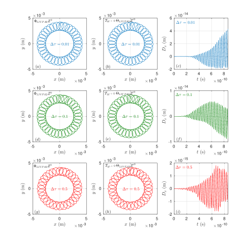
Figure 1: Orbits given by 2-order LIVPA $\Phi_{2}$ in different Lorentz frames. The results in (a), (b) and (c) are simulated with the step-length $\Delta\tau=0.01$, results in d, e and f are calculated by $\Delta\tau=0.1$, and results in g, h and i are calculated by $\Delta\tau=0.5$. The differences between the results calculated in rest and moving frames are on the order of machine precision.

In figure 1, we plot the first turn of the orbit and $D_{x}$ is on the order of machine precision. The differences between the results obtained in different Lorentz inertial frames by LIVPAs result from the machine truncation errors. As the increase of iteration times, the accumulation of machine errors cannot be avoided. Here, we analyze the accumulation of machine errors by studying the magnitude of $\left|D_{x}\right|/R_{0}$ in terms of iteration step number, see Fig. 2. The step length is set as $\Delta\tau=0.1$. The same processes are calculated by using 2-order LIVPA, 4-order LIVPA, and the 2-order implicit midpoint canonical symplectic algorithm (IMCSA). The IMCSA is obtained by discretizing the 4-dimensional Lorentz invariant Hamiltonian equation of charged particles [40] using the implicit mid-point symplectic scheme. For both cases, the value of $\left|D_{x}\right|/R_{0}$ is on the magnitude of machine error at the beginning and finally reaches $10^{-5}$ which is still a negligible value after $10^{6}$ iterations.

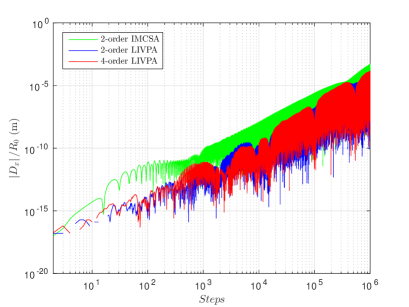
Figure 2: Evolution of $\left|D_{x}\right|/R_{0}$ as the increase of iteration steps. The step-length is set as $\Delta\tau=0.1$. The accumulations of the 2-order LIVPA (blue line), the 4-order LIVPA (red line), and the implicit midpoint canonical symplectic algorithm (IMCSA, green line) have the same trend. After $10^{6}$ iterations, the order of $D_{x}$ is still ignorable compared with $R_{0}$. The IMCSA, is also a LIA, is obtained by discretizing the 4-dimensional Lorentz invariant Hamiltonian equation of charged particles [40] using the implicit mid-point symplectic scheme.

To compare with LIVPAs, we calculate the same process by use of the 2-order explicit canonical symplectic algorithm (ECSA) given in Ref. [24]. This algorithm is built based on generating function method during which the invariant Hamiltonian is divided into 7 parts. As we have discussed in Sec. 2, the splitting method can easily break the Lorentz invariance of continuous systems. In Figure 3, the results in different frames of $\Phi_{ECSA2}$ are plotted. When we set the step length as $\Delta\tau=0.01$, the differences of $x$-coordinate calculated by 2-order ECSA in $\mathcal{O}$ and $\mathcal{O}^{\prime}$ are on the order of $R_{0}$, see Fig. 3c. Especially, as we increase $\Delta\tau$ to $0.1$, ECSA becomes unstable in $\mathcal{O}^{\prime}$ and gives incorrect results, see Fig. 3e. Figure 3 implies that the 2-order ECSA is not Lorentz invariant and one should be very careful to use ECSA in moving frames even though it possesses secular stability in the rest frame.

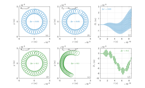
Figure 3: Orbits given by 2-order ECSA given in Ref. [24] in different Lorentz frames. The results in (a), (b) and (c) are simulated with the step-length $\Delta\tau=0.01$, while results in d, e and f are calculated by $\Delta\tau=0.1$. The position difference in two frames is comparable to $R_{0}$ when $\Delta\tau=0.01$, and ECSA becomes unstable in the frame $\mathcal{O}^{\prime}$ for $\Delta\tau=0.1$.

The Vay scheme [38] and the Higuera-Cary scheme [31] can preserve the $\mathbf{E}\times\mathbf{B}$ velocity in different Lorentz frames. Both methods show excellent secular stabilities for simulating relativistic charged particles [30]. Here, we use them to solve the same process in Fig. 1. In $\mathcal{O}$ and $\mathcal{O}^{\prime}$, long-term stable orbits can be obtained by both algorithms. Therefore, in figure 4, we only depict the first major turn. The time step is denoted by $\Delta t$ and $\Delta t^{\prime}$ in $\mathcal{O}$ and $\mathcal{O}^{\prime}$, respectively. In the case of $\Delta t=\Delta t^{\prime}=0.1$, regardless of the small deviations, the results in different frames are consistent, see Figs. 4a and c. As the step length increases to $0.5$, however, we can see significant differences between the red and blue lines. The results show that, Vay’s and Higuera-Cary’s method have better Lorentz invariance for small step length. As the step length increases, even though the global stability still holds, the Lorentz invariance can be broken, which might result from the growth of higher order terms mentioned in Ref. [31]. For LIVPAs, however, the reference-independent property is not affected by the step length, see Fig. 1.

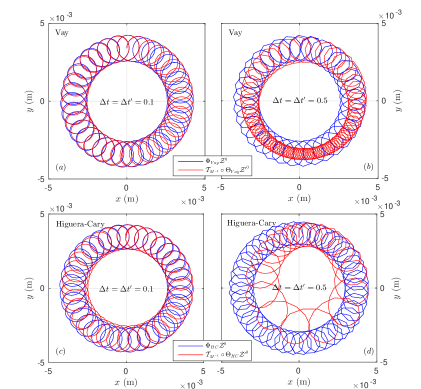
Figure 4: The orbits calculated by Vay’s method [38] and the Higuera-Cary method [31]. Results of Vay’s method are depicted in (a) and (b), while results of the Higuera-Cary method are plotted in (c) and (d). Blue lines give the orbit obtained in frame $\mathcal{O}$ and red lines show the results in frame $\mathcal{O}^{\prime}$. Both methods show better reference-independency for small step length. As the step length increases, the red lines show obvious deviation from blue lines, which shows that Vay’s and Higuera-Cary’s method are not Lorentz invariant. However, both algorithms possess long-term stability in different step length.

5.2 Long-term stability

Through conserving the volume of phase space, the algorithms perform better in secular simulations compared with traditional algorithms like the Newton method, the Runge-Kutta method [33, 42, 34, 35, 41]. Here we compare the secular stabilities of 2-order LIVPA $\Phi_{2}$ with the Lorentz invariant 4-order Runge-Kutta (RK4) method. The Lorentz invariant RK4 method is obtained by discretizing Eq. 13 using the 4-order Runge-Kutta method. Because the discretization keeps the integrity of all the 4-dimensional geometric objects, the resulting method is Lorentz invariant, which can also be proven numerically in figure 5.

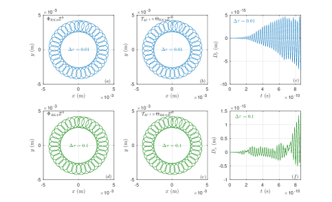
Figure 5: Orbits given by 4-order Lorentz invariant Runge-Kutta method in different Lorentz frames. The results in (a), (b) and (c) are simulated with the step-length $\Delta\tau=0.01$, while results in d, e and f are calculated by $\Delta\tau=0.1$. The results show that the 4-order Runge-Kutta method is Lorentz invariant if it is directly used to discrete the invariant form of the Lorentz force equation, namely, Eq. 13.

For a charged particle moving in static field, there are two important invariants, namely, the mass-shell

$$\mathcal{H}=g_{\alpha\beta}p^{\alpha}p^{\beta}=\gamma^{2}-{\bf p}^{2}\equiv 1\,,$$ (59)

and the energy of the particle

$$H=\gamma+\varphi=\sqrt{1+\mathbf{p}^{2}}+\varphi\,,$$ (60)

In figure 6, the long-term error evolutions of the mass shell $\mathcal{H}\left(\mathcal{Z}\right)$ and the particle energy $H\left(\mathcal{Z}\right)$ simulated by $\Phi_{2}$ and RK4 are depicted. In the case of the mass shell in Fig. 6a, the error of mass shell grows significantly to 1 for RK4, while the error given by 2-order LIVPA is limited near 0. In the case of the particle energy in Fig. 6b, the energy calculated by RK4 decreases 30% after $5\times 10^{6}$ steps, but the energy obtained by $\Phi_{2}$ conserves well. Therefore, the long-term stability of 2-order LIVPA is better than RK4, even though its order is smaller. We also depict the orbits at different moments obtained by 2-order LIVPA and RK4 in figure 7. The orbits calculated by 2-order LIVPA are depicted in Fig. 7a, which remains stable after $5\times 10^{6}$ iterations. For RK4, however, because of the accumulations of numerical errors of RK4, the radius of rotation on minor period keeps shrinking and incorrect orbits are obtained after long-term simulation, see Fig. 7b.

Figure 6: Long-term error evolutions of the mass shell (a) and the particle energy (b) calculated by 2-order LIVPA and 4-order Runge-Kutta. The results of 2-order LIVPA are depicted by blue lines, while the results of Runge-Kutta method are plotted by red lines. The total number of steps is $5\times 10^{6}$. The definitions of errors are $\Delta\mathcal{H}=\mathcal{H}\left(n\Delta\tau\right)-\mathcal{H}_{0}$ and $\Delta H=H\left(n\Delta\tau\right)-H_{0}$. The step length is $\Delta\tau=0.1$.

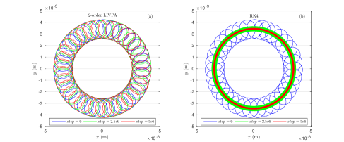
Figure 7: Orbits calculated by 2-order LIVPA (a) and 4-order Runge-Kutta (b) at different moments. The total number of steps is $5\times 10^{6}$ and the step length is set as $\Delta\tau=0.1$.

5.3 Convergence rate of LIVPAs

In Sec. 4, we have constructed several LIVPAs with different orders via different composing procedures. In order to verify their orders, we perform convergence analysis on the 1-order LIVPA $\Phi_{1}$, 2-order LIVPA $\Phi_{2}$, and 4-order LIVPA $\Phi_{4}$. The results are depicted in figure 8. The sequences of energy error $\Delta H$ are calculated from $\tau=0$ to $\tau=10$, and the infinity norm of $\Delta H/H_{0}$ is used to plot the convergence rate. The red line is the convergence rate of $\Phi_{1}$. It has the same slope with the function $10^{-10}\Delta\tau$, which implies $\Phi_{1}$ is a 1-order algorithm. Similarly, $\Phi_{2}$, plotted by the green line, can be proven to be a 2-order algorithm via compared with the reference function $10^{-10}\Delta\tau^{2}$. $\Phi_{4}$ is a 4-order scheme according to the blue line. Because the value of $\Delta H/H_{0}$ reaches machine errors, the convergence rate of $\Phi_{4}$ slows down as the step length becomes very small, see the last point of the blue line at $\Delta\tau=10^{-2}$.

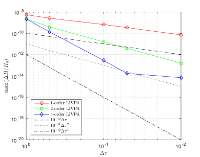
Figure 8: Convergence rates of 1-order LIVPA $\Phi_{1}$, 2-order LIVPA $\Phi_{2}$, and 4-order LIVPA $\Phi_{4}$. The sequences of energy error $\Delta H$ are calculated from $\tau=0$ to $\tau=10$, and the infinity norm of $\Delta H/H_{0}$ is used to plot the convergence rate. The three black lines with different slope are reference functions with 1-order, 2-order, and 4-order convergence rates respectively.

6 Conclusion

In this paper, we study the constructions of explicit Lorentz invariant volume-preserving algorithms for relativistic charged particle dynamics. Through introducing a splitting reference frame (SRF), we prove that the corresponding splitting operation can avoid breaking the Lorentz invariance of the original system. By use of this procedure, we build explicit LIVPAs with different orders. The Lorentz invariant properties of LIVPAs are tested in a typical electromagnetic field configuration, which shows that LIVPAs possess reference-independent secular stabilities. It is proven that the Hamiltonian splitting technique for constructing the explicit symplectic algorithms [24] breaks the Lorentz invariance. Compared with the Vay scheme [38] and the Higuera-Cary scheme [31], the benefits of LIVPAs are also obviously reflected. The reference-independency of LIVPAs is not affected by the configurations of step length, while both Vay and Higuera-Cary methods show the decreases of accuracy in different frames when the step length grows. Meanwhile, long-term behaviors of LIVPAs show better than the Runge-Kutta method in resolving the motion constants such as the mass-shell and the particle energy. Therefore, LIVPAs have better performances when simulating nonlinear multi-scale processes. We also provide the numerical convergence analysis to LIVPAs, which proves the ability of the Lorentz invariant splitting method in constructing high order explicit schemes.

The work in this paper extends the method introduced in Ref. [39] in which the integrity of geometric objects is necessary to construct Lorentz invariant algorithms. We generalize the idea to a more flexible level, that even though the geometric objects in 4-dimensional spacetime are broken, the Lorentz invariance of algorithms still holds. The combination of the splitting technique and the Lorentz invariant method provides a convenient way to build advanced algorithms with high orders. Additionally, generally speaking, as the orders of algorithms increase, it will be more difficult to implement adaptive time step optimization. Especially, constructing structure-preserving algorithms with adaptive time step is still a difficult task. Some works have been done by use of the time transformation method [21, 43] which should transform the original system into a new form. The results given by symplectic algorithms of the new system in which the step length are still fixed are equivalent to results by adaptive step length in the original system. In future work, more works will be done to study and apply the LIVPAs to key physical problems in different areas, and the usage of LIVPAs in Particle-in-Cell codes will also be studied.

Appendix

In this appendix, we provide the detailed derivations of Eqs. 39, 40, and 44. According to the definitions of $\mathcal{K}_{\ \beta}^{\alpha}$ and $\mathcal{R}_{\ \beta}^{\alpha}$, it is readily to find that $\left(\mathcal{K}_{\ \beta}^{\alpha}\right)^{3}=\left(E^{r}\right)^{2}\mathcal{K}_{\ \beta}^{\alpha}$ and $\left(\mathcal{R}_{\ \beta}^{\alpha}\right)^{3}=-\left(B^{r}\right)^{2}\mathcal{R}_{\ \beta}^{\alpha}$. Therefore, considering that $E^{r}$ and $B^{r}$ are scalar fields, we have $\left(K_{\ \beta}^{\alpha}\right)^{3}=L\left(\mathcal{K}_{\ \beta}^{\alpha}\right)^{3}L^{-1}=L\left(E^{r}\right)^{2}\mathcal{K}_{\ \beta}^{\alpha}L^{-1}=\left(E^{r}\right)^{2}L\mathcal{K}_{\ \beta}^{\alpha}L^{-1}=\left(E^{r}\right)^{2}K_{\ \beta}^{\alpha}$. One should notice that, $E^{r}$ is a function in frame $\mathcal{O}^{r}$ while $K_{\ \beta}^{\alpha}$ is the matrix evaluated in frame $\mathcal{O}$. When we calculate the value of $\left(K_{\ \beta}^{\alpha}\right)^{3}$ at $x^{\alpha}$ in frame $\mathcal{O}$, the input of value of $E^{r}$ should be $L^{-1}x^{\alpha}$. From the viewpoint of manifold, $x^{\alpha}$ and $L^{-1}x^{\alpha}$ are different coordinates of the same point on manifold. Similarly, we can also obtain $\left(R_{\ \beta}^{\alpha}\right)^{3}=-\left(B^{r}\right)^{2}R_{\ \beta}^{\alpha}$.

We first prove that $\exp\left(\tau\tilde{q}K_{\ \beta}^{\alpha}\right)=I_{\ \beta}^{\alpha}+\frac{\sinh\left(\tau\tilde{q}E^{r}\right)}{E^{r}}K_{\ \beta}^{\alpha}+\frac{\cosh\left(\tau\tilde{q}E^{r}\right)-1}{\left(E^{r}\right)^{2}}S_{\ \beta}^{\alpha}$ in Eq. 39. Using $\left(K_{\ \beta}^{\alpha}\right)^{2}=S_{\ \beta}^{\alpha}$ and $\left(K_{\ \beta}^{\alpha}\right)^{3}=\left(E^{r}\right)^{2}K_{\ \beta}^{\alpha}$, we have

$$\exp\left(\tau\tilde{q}K_{\ \beta}^{\alpha}\right) = I_{\ \beta}^{\alpha}+\tau\tilde{q}K_{\ \beta}^{\alpha}+\frac{\left(\tau\tilde{q}K_{\ \beta}^{\alpha}\right)^{2}}{2!}+\frac{\left(\tau\tilde{q}K_{\ \beta}^{\alpha}\right)^{3}}{3!}+\cdots$$ (61)

$$= I_{\ \beta}^{\alpha}+\tau\tilde{q}K_{\ \beta}^{\alpha}+\frac{\left(\tau\tilde{q}\right)^{2}}{2!}K_{\ \beta}^{\alpha}+\frac{\left(\tau\tilde{q}\right)^{3}\left(E^{r}\right)^{2}}{3!}K_{\ \beta}^{\alpha}+\frac{\left(\tau\tilde{q}\right)^{3}\left(E^{r}\right)^{2}}{4!}S_{\ \beta}^{\alpha}+\cdots$$

$$= I_{\ \beta}^{\alpha}+\frac{1}{E^{r}}\left(\tau\tilde{q}E^{r}+\frac{\left(\tau\tilde{q}E^{r}\right)^{3}}{3!}+\frac{\left(\tau\tilde{q}E^{r}\right)^{5}}{5!}+\cdots\right)K_{\ \beta}^{\alpha}$$

$$+\frac{1}{\left(E^{r}\right)^{2}}\left(-1+1+\frac{\left(\tau\tilde{q}E^{r}\right)^{2}}{2!}+\frac{\left(\tau\tilde{q}E^{r}\right)^{4}}{4!}+\cdots\right)S_{\ \beta}^{\alpha}$$

$$= I_{\ \beta}^{\alpha}+\frac{1}{E^{r}}\frac{e^{\tau\tilde{q}E^{r}}-e^{-\tau\tilde{q}E^{r}}}{2}K_{\ \beta}^{\alpha}+\frac{1}{\left(E^{r}\right)^{2}}\left(-1+\frac{e^{\tau\tilde{q}E}+e^{-\tau\tilde{q}E}}{2}\right)S_{\ \beta}^{\alpha}$$

$$= I_{\ \beta}^{\alpha}+\frac{\sinh\left(\tau\tilde{q}E^{r}\right)}{E^{r}}K_{\ \beta}^{\alpha}+\frac{\cosh\left(\tau\tilde{q}E^{r}\right)-1}{\left(E^{r}\right)^{2}}S_{\ \beta}^{\alpha}\,.$$

The derivation of Eqs. 40 is similar. The equation $\exp\left(\tau\tilde{q}R_{\ \beta}^{\alpha}\right)=I_{\ \beta}^{\alpha}+\frac{\sin\left(\tau\tilde{q}B^{r}\right)}{B^{r}}R_{\ \beta}^{\alpha}+\frac{1-\cos\left(\tau\tilde{q}B^{r}\right)}{\left(B^{r}\right)^{2}}P_{\ \beta}^{\alpha}$ can be proven using $\left(R_{\ \beta}^{\alpha}\right)^{2}=P_{\ \beta}^{\alpha}$ and $\left(R_{\ \beta}^{\alpha}\right)^{3}=-\left(B^{r}\right)^{2}R_{\ \beta}^{\alpha}$ as follows,

$$\exp\left(\tau\tilde{q}R_{\ \beta}^{\alpha}\right) = I_{\ \beta}^{\alpha}+\tau\tilde{q}R_{\ \beta}^{\alpha}+\frac{\left(\tau\tilde{q}R_{\ \beta}^{\alpha}\right)^{2}}{2!}+\frac{\left(\tau\tilde{q}R_{\ \beta}^{\alpha}\right)^{3}}{3!}+\cdots$$ (62)

$$= I_{\ \beta}^{\alpha}+\tau\tilde{q}R_{\ \beta}^{\alpha}+\frac{\left(\tau\tilde{q}\right)^{2}}{2!}P_{\ \beta}^{\alpha}-\frac{\left(\tau\tilde{q}\right)^{3}\left(B^{r}\right)^{2}}{3!}R_{\ \beta}^{\alpha}-\frac{\left(\tau\tilde{q}\right)^{3}\left(B^{r}\right)^{2}}{4!}P_{\ \beta}^{\alpha}+\cdots$$

$$= I_{\ \beta}^{\alpha}+\frac{1}{B^{r}}\left(\tau\tilde{q}B^{r}-\frac{\left(\tau\tilde{q}B^{r}\right)^{3}}{3!}+\frac{\left(\tau\tilde{q}B^{r}\right)^{5}}{5!}-\cdots\right)R_{\ \beta}^{\alpha}$$

$$-\frac{1}{\left(B^{r}\right)^{2}}\left(-1+1-\frac{\left(\tau\tilde{q}B^{r}\right)^{2}}{2!}+\frac{\left(\tau\tilde{q}B^{r}\right)^{4}}{4!}-\cdots\right)P_{\ \beta}^{\alpha}$$

$$= I_{\ \beta}^{\alpha}+\frac{\sin\left(\tau\tilde{q}B^{r}\right)}{B^{r}}R_{\ \beta}^{\alpha}+\frac{1-\cos\left(\tau\tilde{q}B^{r}\right)}{\left(B^{r}\right)^{2}}P_{\ \beta}^{\alpha}\,.$$

The explicit form of Cayley transformation in Eq. 44 can be proven as follows,

$$\mathrm{cay}\left(\Delta\tau\tilde{q}R_{\ \beta}^{\alpha}\right) = \left(I_{\ \beta}^{\alpha}-aR_{\ \beta}^{\alpha}\right)^{-1}\left(I_{\ \beta}^{\alpha}+aR_{\ \beta}^{\alpha}\right)$$ (63)

$$= \left[I_{\ \beta}^{\alpha}+aR_{\ \beta}^{\alpha}+\left(aR_{\ \beta}^{\alpha}\right)^{2}+\left(aR_{\ \beta}^{\alpha}\right)^{3}+\cdots\right]\left(I_{\ \beta}^{\alpha}+aR_{\ \beta}^{\alpha}\right)$$

$$= \left[I_{\ \beta}^{\alpha}+\left(1-\left(aB^{r}\right)^{2}+\left(aB^{r}\right)^{4}-\cdots\right)aR_{\ \beta}^{\alpha}\right.$$

$$\left.+\left(1-\left(aB^{r}\right)^{2}+\left(aB^{r}\right)^{4}-\cdots\right)a^{2}P_{\ \beta}^{\alpha}\right]\left(I_{\ \beta}^{\alpha}+aR_{\ \beta}^{\alpha}\right)$$

$$= \left[I_{\ \beta}^{\alpha}+\frac{a}{1+\left(aB^{r}\right)^{2}}R_{\ \beta}^{\alpha}+\frac{a^{2}}{1+\left(aB^{r}\right)^{2}}P_{\ \beta}^{\alpha}\right]\left(I_{\ \beta}^{\alpha}+aR_{\ \beta}^{\alpha}\right)$$

$$= \left(I_{\ \beta}^{\alpha}+\frac{2a}{1+\left(aB^{r}\right)^{2}}R_{\ \beta}^{\alpha}+\frac{2a^{2}}{1+\left(aB^{r}\right)^{2}}P_{\ \beta}^{\alpha}\right)\,.$$

References

References

- [1] K. Feng, Difference schemes for hamiltonian formalism and symplectic geometry, Journal of Computational Mathematics 4 (3) (1986) 279–289.
- [2] E. Forest, R. D. Ruth, Fourth-order symplectic integration, Physica D 43 (1) (1990) 105.
- [3] R. I. McLachlan, G. R. W. Quispel, Geometric integrators for ODEs, J. Phys. A: Math. Gen. 39 (19) (2006) 5251.
- [4] J. Candy, W. Rozmus, A symplectic integration algorithm for separable Hamiltonian functions, J. Comput. Phys. 92 (1) (1991) 230.
- [5] R. I. McLachlan, P. Atela, The accuracy of symplectic integrators, Nonlinearity 5 (2) (1992) 541.
- [6] J. R. Cary, I. Doxas, An explicit symplectic integration scheme for plasma simulations, Journal of Computational Physics 107 (1) (1993) 98.
- [7] Z. Shang, Kam theorem of symplectic algorithms for Hamiltonian systems, Numerische Mathematik 83 (3) (1999) 477–496.
- [8] H. Qin, X. Guan, Variational symplectic integrator for long-time simulations of the guiding-center motion of charged particles in general magnetic fields, Phys. Rev. Lett. 100 (3) (2008) 035006.
- [9] J. Li, H. Qin, Z. Pu, L. Xie, S. Fu, Variational symplectic algorithm for guiding center dynamics in the inner magnetosphere, Phys. Plasmas 18 (5) (2011) 052902.
- [10] M. Kraus, Variational integrators in plasma physics, arXiv preprint arXiv:1307.5665.
- [11] J. Xiao, J. Liu, H. Qin, Z. Yu, N. Xiang, Variational symplectic particle-in-cell simulation of nonlinear mode conversion from extraordinary waves to Bernstein waves, Phys. Plasmas 22 (9) (2015) 092305.
- [12] H. Qin, J. Liu, J. Xiao, R. Zhang, Y. He, Y. Wang, Y. Sun, J. W. Burby, L. Ellison, Y. Zhou, Canonical symplectic particle-in-cell method for long-term large-scale simulations of the Vlasov–Maxwell equations, Nucl. Fusion 56 (1) (2015) 014001.
- [13] J. Qiang, Symplectic multiparticle tracking model for self-consistent space-charge simulation, Physical Review Accelerators and Beams 20 (1) (2017) 014203.
- [14] B. Shadwick, A. Stamm, E. Evstatiev, Variational formulation of macro-particle plasma simulation algorithms, Phys. Plasmas 21 (5) (2014) 055708.
- [15] S. D. Webb, A spectral canonical electrostatic algorithm, Plasma Phys. Controlled Fusion 58 (3) (2016) 034007.
- [16] Y. Zhou, H. Qin, J. W. Burby, A. Bhattacharjee, Variational integration for ideal magnetohydrodynamics with built-in advection equations, Phys. Plasmas 21 (10) (2014) 102109.
- [17] Y. Zhou, Y.-M. Huang, H. Qin, A. Bhattacharjee, Formation of current singularity in a topologically constrained plasma, Physical Review E 93 (2) (2016) 023205.
- [18] J. Xiao, H. Qin, P. J. Morrison, J. Liu, Z. Yu, R. Zhang, Y. He, Explicit high-order noncanonical symplectic algorithms for ideal two-fluid systems, Phys. Plasmas 23 (11) (2016) 112107.
- [19] U. M. Ascher, R. I. McLachlan, Multisymplectic box schemes and the Korteweg–de Vries equation, Applied Numerical Mathematics 48 (3-4) (2004) 255.
- [20] J.-Q. Sun, M.-Z. Qin, Multi-symplectic methods for the coupled 1d nonlinear Schrödinger system, Comput. Phys. Commun. 155 (3) (2003) 221.
- [21] E. Hairer, C. Lubich, G. Wanner, Geometric numerical integration: structure-preserving algorithms for ordinary differential equations, Vol. 31, Springer Science & Business Media, 2006.
- [22] J. Xiao, H. Qin, J. Liu, Structure-preserving geometric particle-in-cell methods for Vlasov-Maxwell systems, Plasma Sci. Technol 20 (11) (2018) 110501.
- [23] R. Zhang, H. Qin, Y. Tang, J. Liu, Y. He, J. Xiao, Explicit symplectic algorithms based on generating functions for charged particle dynamics, Phys. Rev. E 94 (1) (2016) 013205.
- [24] R. Zhang, Y. Wang, Y. He, J. Xiao, J. Liu, H. Qin, Y. Tang, Explicit symplectic algorithms based on generating functions for relativistic charged particle dynamics in time-dependent electromagnetic field, Phys. Plasmas 25 (2) (2018) 022117.
- [25] Z. Zhou, Y. He, Y. Sun, J. Liu, H. Qin, Explicit symplectic methods for solving charged particle trajectories, Phys. Plasmas 24 (5) (2017) 052507.
- [26] Y. He, Z. Zhou, Y. Sun, J. Liu, H. Qin, Explicit K-symplectic algorithms for charged particle dynamics, Phys. Lett. A 381 (6) (2016) 568–573.
- [27] J. Xiao, H. Qin, Explicit high-order gauge-independent symplectic algorithms for relativistic charged particle dynamics, Comput. Phys. Commun. 241 (2019) 19.
- [28] C. K. Birdsall, A. B. Langdon, Plasma physics via computer simulation, CRC Press, 2004.
- [29] K. Germaschewski, W. Fox, S. Abbott, N. Ahmadi, K. Maynard, L. Wang, H. Ruhl, A. Bhattacharjee, The plasma simulation code: A modern particle-in-cell code with patch-based load-balancing, Journal of Computational Physics 318 (2016) 305.
- [30] B. Ripperda, F. Bacchini, J. Teunissen, C. Xia, O. Porth, L. Sironi, G. Lapenta, R. Keppens, A comprehensive comparison of relativistic particle integrators, The Astrophysical Journal Supplement Series 235 (1) (2018) 21.
- [31] A. V. Higuera, J. R. Cary, Structure-preserving second-order integration of relativistic charged particle trajectories in electromagnetic fields, Phys. Plasmas 24 (5) (2017) 052104.
- [32] A. Matsuyama, M. Furukawa, High-order integration scheme for relativistic charged particle motion in magnetized plasmas with volume preserving properties, Comput. Phys. Commun. 220 (2017) 285.
- [33] H. Qin, S. Zhang, J. Xiao, J. Liu, Y. Sun, W. M. Tang, Why is Boris algorithm so good?, Phys. Plasmas 20 (8) (2013) 084503.
- [34] Y. He, Y. Sun, J. Liu, H. Qin, Volume-preserving algorithms for charged particle dynamics, J. Comput. Phys. 281 (2015) 135.
- [35] R. Zhang, J. Liu, H. Qin, Y. Wang, Y. He, Y. Sun, Volume-preserving algorithm for secular relativistic dynamics of charged particles, Phys. Plasmas 22 (4) (2015) 044501.
- [36] Y. He, Y. Sun, R. Zhang, Y. Wang, J. Liu, H. Qin, High order volume-preserving algorithms for relativistic charged particles in general electromagnetic fields, Phys. Plasmas 23 (9) (2016) 092109.
- [37] J. L. Vay, Noninvariance of space- and time-scale ranges under a lorentz transformation and the implications for the study of relativistic interactions, Phys. Rev. Lett. 98 (13) (2007) 130405.
- [38] J. L. Vay, Simulation of beams or plasmas crossing at relativistic velocity, Phys. Plasmas 15 (5) (2008) 056701.
- [39] Y. Wang, J. Liu, H. Qin, Lorentz covariant canonical symplectic algorithms for dynamics of charged particles, Phys. Plasmas 23 (12) (2016) 122513.
- [40] J. D. Jackson, Classical electrodynamics, Vol. 3, Wiley New York etc., 1962.
- [41] R. Zhang, J. Liu, H. Qin, Y. Tang, Y. He, Y. Wang, Application of lie algebra in constructing volume-preserving algorithms for charged particles dynamics, Communications in Computational Physics 19 (5) (2016) 1397.
- [42] C. L. Ellison, J. Finn, H. Qin, W. M. Tang, Development of variational guiding center algorithms for parallel calculations in experimental magnetic equilibria, Plasma Phys. Controlled Fusion 57 (5) (2015) 054007.
- [43] Y. Shi, Y. Sun, Y. Wang, J. Liu, Study of adaptive symplectic methods for simulating charged particle dynamics, Journal of Computational Dynamics 6 (2) (2019) 429.