Operation and characterization of a windowless gas jet target in high-intensity electron beams

Abstract

A cryogenic supersonic gas jet target was developed for the MAGIX experiment at the high-intensity electron accelerator MESA. It will be operated as an internal, windowless target in the energy-recovering recirculation arc of the accelerator with different target gases, e.g., hydrogen, deuterium, helium, oxygen, argon, or xenon. Detailed studies have been carried out at the existing A1 multi-spectrometer facility at the electron accelerator MAMI. This paper focuses on the developed handling procedures and diagnostic tools, and on the performance of the gas jet target under beam conditions. Considering the special features of this type of target, it proves to be well suited for a new generation of high-precision electron scattering experiments at high-intensity electron accelerators.

1 Introduction

Electron scattering is a very powerful tool for studying the structure of nucleons and atomic nuclei [1]. Investigations of form factors, polarizabilities, and of the excitation spectra of hadrons are being performed to reach a detailed description of low-energy phenomena on the basis of quantum chromodynamics. The use of electron beams as a probe provides a clean reaction mechanism and allows for a high precision, which often is limited by technical factors rather than by the interpretation of the measured observables in physical terms. When, for instance, the systematic uncertainty of a cross section measurement should be reduced below the 1-percent level, a typical limiting factor is related to the considerable thickness of the target material resulting in energy-loss straggling and multiple small-angle scattering. In case of targets with gas enclosed in cells, irreducible backgrounds can be introduced by the interaction of the electron beam with surrounding structures such as cell walls or foils. Therefore, the use of very thin and windowless targets is highly desirable (see for instance [2]), but poses the challenge of relatively small luminosities and count rates for beam currents available at conventional electron accelerators. A new generation of high-intensity electron accelerators will allow to overcome this shortcoming.

One of these new accelerators will be MESA (Mainz Energy-Recovering Superconducting Accelerator), an Energy Recovery Linac (ERL), currently under construction in Mainz, Germany [3, 4]. In the ERL mode, the beam is, after passing the target, guided back into the superconducting radio-frequency system with a phase shift of 180^∘, so that the electrons transfer most of their energy back to the accelerating structures. This scheme provides a power-efficient beam acceleration with a maximum beam energy of $E=105\,\mathrm{MeV}$ and a maximum beam current of $I=1000\,\mathrm{\mu A}$ or higher.

The maximum acceptable multiple scattering contribution for the ERL mode limits the areal thickness of the target to less than $\rho_{\text{areal}}\approx 10^{20}\,\mathrm{atoms/cm^{2}\cdot\nicefrac{{1}}{{Z^{2}}}}$ with $Z$ being the atomic number of the target material. In addition, the destructive heat deposition of high beam currents makes it unfeasible to have the beam passing through target cell walls.

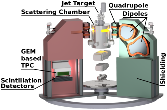
Figure 1: Overview of the planned MAGIX spectrometer setup at the ERL arc of the MESA accelerator. The gas jet target will be mounted in a scattering chamber with a pumping system connected to it. The two magnetic spectrometers in quadrupole-dipole-dipole magnetic configuration can rotate around the target. Their focal planes will be equipped with TPCs for tracking, and scintillation detectors for trigger, timing, and particle identification purposes.

The MAinz Gas Injection target eXperiment MAGIX will employ a multi-purpose spectrometer system in the ERL arc of MESA and a gas jet target at its center. The two high-resolution magnetic spectrometers will be used for the detection of scattered electrons and produced particles. Their focal planes will be equipped with TPCs (time projection chambers) with GEM (gas electron multiplier) readout for tracking [5], and with a dedicated trigger and veto system consisting of a segmented layer of plastic scintillation detectors and a flexible number of additional layers and lead absorbers. Figure 1 shows a schematic of the planned MAGIX setup.

While the MESA accelerator and the experimental site for the MAGIX setup are currently under construction, the gas jet target was already developed and tested at the University of Münster [6]. In 2017 it could be installed and successfully operated at the existing A1 multi-spectrometer setup at the Mainz Microtron (MAMI) electron accelerator in Mainz, Germany.

The optimization of the target system was crucial to realize its full potential and to open the avenue for innovative precision experiments. The combination of a low beam energy, a thin and nearly point-like target and a high beam current is ideally suited to perform novel precision experiments in nuclear, hadron, and particle physics. In addition, the target allows for the detection of low-energy recoil nuclei inside the scattering chamber.

One major motivation is the study of form factors of nucleons and nuclei in elastic electron scattering at low momentum transfers $Q^{2}$ reaching down to below $10^{-4}\,\mathrm{GeV^{2}}$, allowing, for instance, a precise determination of the proton charge radius. Key element for the success of this type of experiments will be the absence of a target cell and, compared to a liquid target, the very low target density, minimizing the irreducible background and effects from energy loss and multiple scattering [7, 8, 9].

With the MAGIX setup, the search for dark photons will be extended to lower dark photon masses than were probed before [10, 11]. In this type of experiments a dark photon $\gamma^{\prime}$ could radiatively be produced off a nuclear target $Z$ via the reaction $e^{-}Z\rightarrow e^{-}Z\gamma^{\prime}$, and a missing mass analysis of coincident $e^{+}e^{-}$ pairs from the decay $\gamma^{\prime}\rightarrow e^{+}e^{-}$ needs to be performed. These searches will be extended to invisible decay channels, in which a dark photon decays via $\gamma^{\prime}\rightarrow\chi\bar{\chi}$ in a pair of light dark matter particles, requiring a missing mass analysis of the scattered electron in coincidence with the recoil nucleus [12, 13].

Furhtermore, the study of reactions of astrophysical importance such as ¹⁶O$(e,e^{\prime}\alpha)^{12}$C, where the $\alpha$-particle is detected with a detector arrangement inside the scattering chamber, will become possible at unprecedented low center-of-mass energies [14, 15].

This paper is organized as follows: Section 2 provides an overview of the experimental setup and the gas jet target. Section 3 describes details of the handling procedures and operating parameters of the target. The gas jet is characterized in Sect. 4. Its areal thickness (Subsect. 4.1) and density (Subsect. 4.2) were deduced from a comparison to a simulation of elastic scattering events. Clustering of the gas jet is discussed in Subsect. 4.3. A sophisticated simulation is described in Subsect. 4.4, and the results are compared to measured profiles from two different nozzle designs in Subsect. 4.5. Section 5 discusses dedicated background studies for electron scattering experiments with this target. The stability of the gas jet is considered in Sect. 6 and the target is compared to other hydrogen targets at electron accelerators in Sect. 7. A summary and an outlook are given in Sect. 8.

2 Experimental setup

2.1 MAMI and A1 multi-spectrometer facility

MAMI delivers electrons with energies of up to $E_{\text{beam}}=1600\,\mathrm{MeV}$ at beam currents of up to $I_{\text{beam}}=100\,\mathrm{\mu A}$ [16, 17, 18, 19]. For experiments at this facility, different types of targets are available, including solid state targets (single foils and stacks), liquid hydrogen and deuterium targets, a high pressure helium target, a polarized ³He target, and a waterfall target.

At the spectrometer setup of the A1 Collaboration, scattered electrons from the interaction of the beam electrons with the target can be detected with the high-resolution magnetic spectrometers A, B, and C, see Fig. 2 for a schematic of spectrometer A. These spectrometers have target length acceptances of $\Delta l=5\,\mathrm{cm}$, solid angle acceptances of $\Delta\Omega=28\,\mathrm{msr}$ (for A and C) and $\Delta\Omega=5.6\,\mathrm{msr}$ (for B), and momentum acceptances of $\Delta p/p=$ 15 % (for B), 20 % (for A), and 25 % (for C). A detailed description of the spectrometers can be found in Ref. [20]. Vertical drift chambers are used for tracking, scintillation detectors for trigger and timing purposes, and a threshold gas Cherenkov detector for discrimination between electrons and pions or muons. The spectrometers have a relative momentum resolution of $\delta p/p\approx 10^{-4}$ and an angular resolution at the target of $\delta\theta/\theta\approx 3\,\mathrm{mrad}$ [20].

The gas jet target was assembled, tested, and operated at the A1 spectrometer setup with $E_{\text{beam}}$ between $195\,\mathrm{MeV}$ and $450\,\mathrm{MeV}$ and at beam currents of up to $I_{\text{beam}}=20\,\mathrm{\mu A}$. A photograph of the experimental setup is shown in Fig. 3.

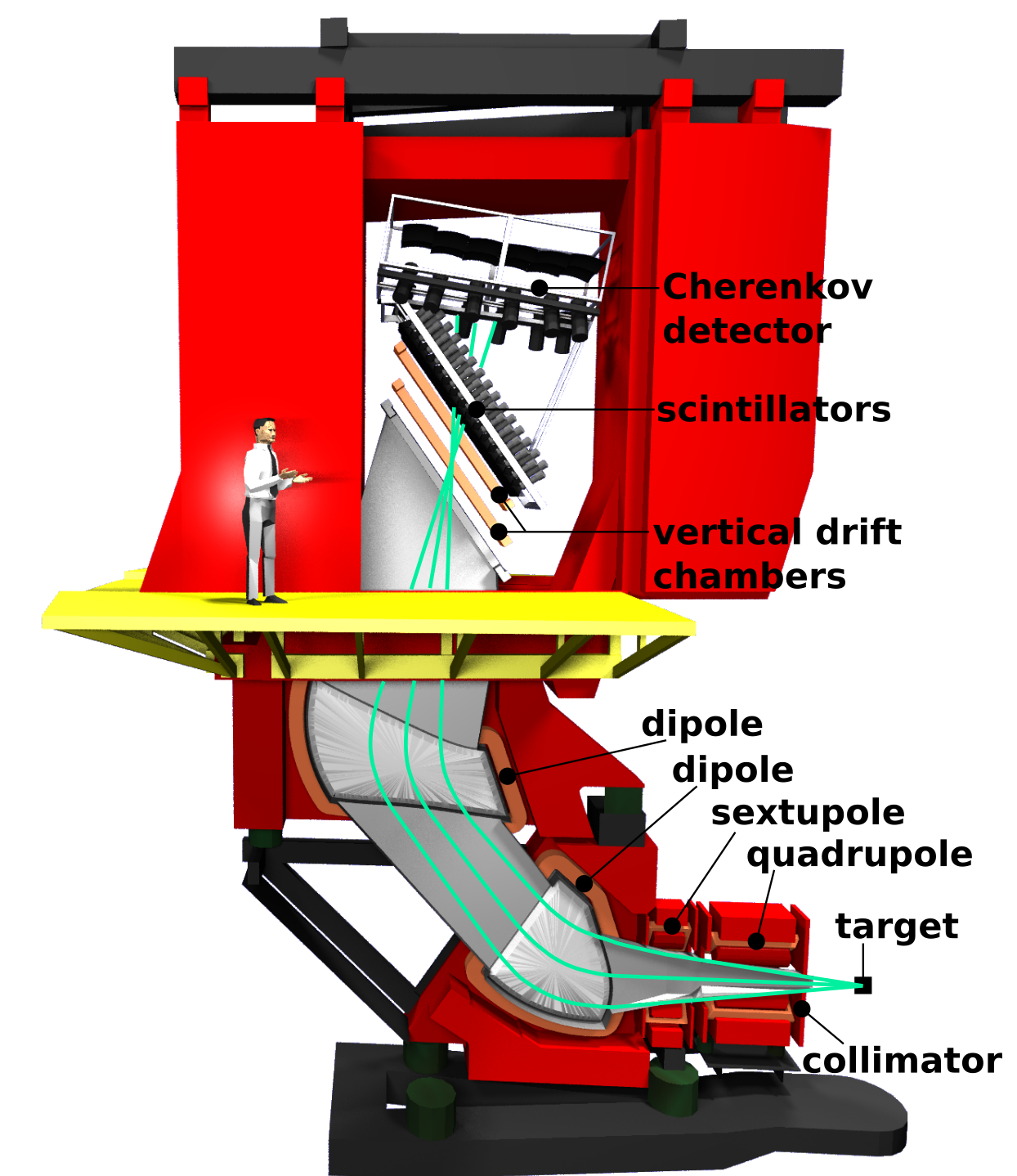
Figure 2: Schematic side view of spectrometer A at the A1 multi-spectrometer setup. The magnets are partly cut open to show pole pieces and coils. The doors of the shielding house are shown in the opened position, exhibiting the detector package. Three trajectories for charged particles coming from the target with identical momentum are shown. The particles enter the spectrometer through a collimator and are guided by the fields of four separate magnets to the focal plane. Their momenta and angles at the target position are reconstructed from the measured tracks across the focal plane. A Cherenkov detector provides electron identification.

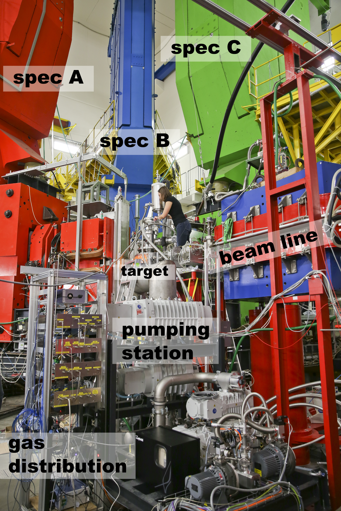
Figure 3: Photograph of the gas jet target mounted at the A1 multi-spectrometer setup. The electron beam enters the cylindrical scattering chamber from the right. Scattered electrons and particles emitted in direction of the spectrometers leave the chamber through Kapton windows. The three magnetic spectrometers can rotate around the target. For the studies presented in this paper, spectrometers A (in red) and B (in blue) were used. Photograph by T. Zimmermann / JGU.

2.2 Electron beam size

In order to determine the width of the electron beam on the gas jet target, a gold-plated tungsten wire with a diameter of $\varnothing=100\,\mathrm{\mu m}$ was moved through the beam using the stepper motor shown in Fig. 10. Since the turning radius $r=106\,\mathrm{mm}$ was relatively large, the rotation of the wire target resulted in an approximately even, horizontal movement of the vertically aligned wire for the small displacements of typically $\Delta x=20\,\mathrm{\mu m}$.

Two spectrometers were set to a kinematic setting corresponding to the quasi-elastic electron scattering off the heavy nuclei of the wire. The variation of the count rates with the wire positions was monitored. From a fit to the distribution of scattering events as a function of the reconstructed position, the horizontal width of the electron beam was determined to be of the order of FWHM $\approx 100\,\mathrm{\mu m}$, see Fig. 4. From the beam spot on the luminescence screen, it was known that the beam was axially symmetric.

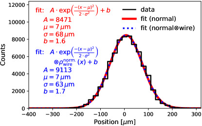
Figure 4: Scattering events as a function of the wire position for data taking periods of $\Delta t=30\,\mathrm{s}$ at each position. A fit with a normal distribution on top of a small offset was performed. For a very thin wire, the width parameter $\sigma$ can be interpreted as the horizontal electron beam width. Including the finite wire size in the fit results in a $10\,\mathrm{\%}$ smaller parameter $\sigma$.

2.3 Fast beam wobbler

A fast beam wobbler, using air-core coils, is installed $12\,\mathrm{m}$ upstream of the target [21] to raster the electron beam horizontally, vertically, or both at the same time. The coils are energized by alternating sine wave currents with frequencies of $f=2.918\,\mathrm{kHz}$ and $f=2.000\,\mathrm{kHz}$, respectively. The displacement of the beam at the target location is approximately proportional to the coil current, which is monitored by means of a bipolar 8-bit analog digital converter (ADC). The displacement distribution, as recorded by the ADC, is shown in Fig. 5 for horizontal wobbling. The figure also shows the cuts that were applied to the vertex position in the following analyses to reduce the bias from the non-uniform distribution.

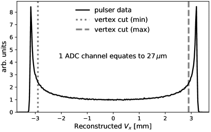
Figure 5: Horizontal displacement distribution of the electron beam at the target location. The wobbler current was recorded by an ADC. The $x$-axis has been calibrated in $\mathrm{mm}$ units.

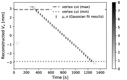
Figure 6: Reconstructed horizontal vertex position as a function of time for a rastered beam during a stepwise movement of the wire target. For each data taking period, the wire position was known, and a fit with a normal distribution was applied to the histogram of the reconstructed vertex position. These data are used to calibrate the wobbler readout conversion from ADC channels to mm, and to estimate the precision of the reconstructed beam displacement.

To calibrate the wobbler readout in terms of displacement at the target position, data were taken for different wire target positions, see Fig. 6. When the displaced beam covered the wire position, the spectrometers registered quasi-elastic scattering events. From the known wire position for each setting, the acquired wobbler ADC values were related to the displacement.

The achievable precision of the position reconstruction for a single scattering event is limited by the finite electron beam width, by the resolution of the wobbler ADC, and by specific instrumental restrictions which are detailed in Ref. [21]. The coil current in the wobbler magnets for a given beam displacement is proportional to the beam energy. Thus, the range of amplitudes within the dynamic range of the ADC changes with beam energy. The typical precision during the electron scattering studies at a beam energy of $E=315\,\mathrm{MeV}$ was $\sigma^{V_{x}}\approx 150\,\mathrm{\mu m}$, and slightly better at $E=450\,\mathrm{MeV}$, cf. Fig. 7.

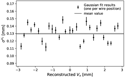
Figure 7: Precision of the position reconstruction as a function of the horizontal displacement. The average precision for this beam energy of $E=450\,\mathrm{MeV}$ was $\sigma^{V_{x}}=130\,\mathrm{\mu m}$.

2.4 Gas jet target

The target for the MAGIX setup as shown in Fig. 8 is a cryogenic supersonic jet target that can be operated with most gases [6]. It was designed to achieve areal thicknesses of more than $\rho_{\text{areal}}\approx 10^{18}\,\mathrm{atoms/cm^{2}}$ when using hydrogen. This requires a gas flow rate of up to $q_{V}=2400\,\mathrm{l_{n}/h}$ while the hydrogen gas has to be cooled down to $T_{0}=40\,\mathrm{K}$. Two systems provide the necessary cooling power. The target gas first enters a booster stage that can be filled with liquid nitrogen to precool the gas. Based on a sophisticated level meter, the nitrogen refill is automated. It is then guided through copper windings that surround the two stages of a cryogenic cold head. To allow a precise temperature regulation, both stages are equipped with heaters and temperature sensors, where the measured temperature at the second stage corresponds to the gas temperature directly in front of the nozzle. Furthermore, the booster stage and the cold head are surrounded by two separate evacuated insulation volumes to minimize the heat conduction with the environment and to minimize the nitrogen consumption within the booster. The cryogenic gas is then pressed through a convergent–divergent nozzle where it is accelerated to supersonic velocities and adiabatically cooled down during the expansion. This results in a supersonic jet that is ejected vertically from the nozzle and is caught several mm below by a funnel-shaped structure, the catcher. The electron beam of the accelerator traverses the gas jet horizontally inside the scattering chamber, resulting in a very compact interaction zone. The target including its technical details and operational parameters is described in Ref. [6] in more detail.

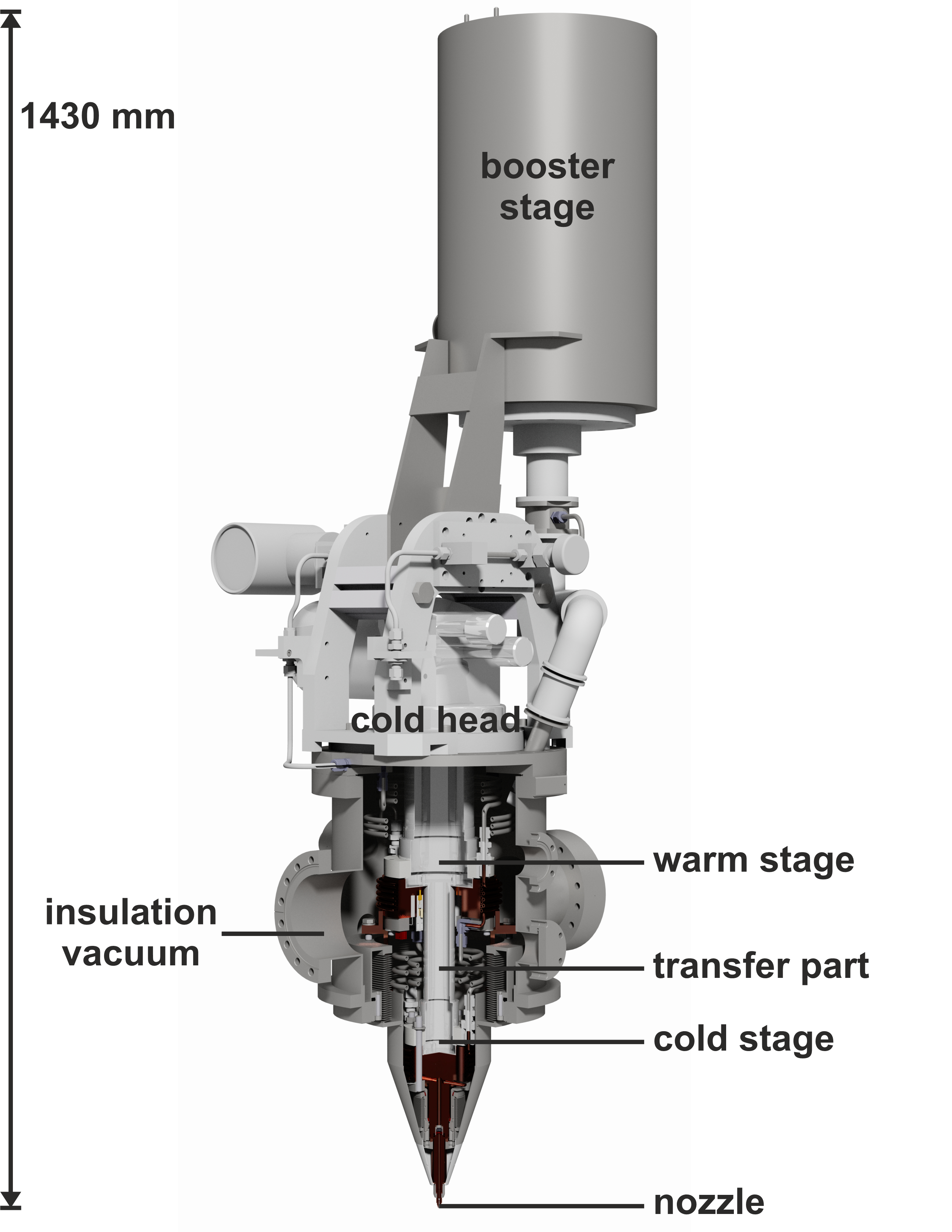
Figure 8: Drawing of the gas jet target for the MAGIX setup. The booster stage can be filled with liquid nitrogen to precool the gas, which is then guided to a two-stage cold head where it reaches a temperature of $T_{0}=40\,\mathrm{K}$ when operated with hydrogen. The convergent–divergent nozzle is mounted on top of an extension which is surrounded by a conical tip to ensure a high angular acceptance for the spectrometers.

Assuming a perfect gas, the velocity of the gas leaving the nozzle can be calculated by

$$v=\sqrt{2c_{p}T_{0}}=\sqrt{2\frac{\kappa}{\kappa-1}\frac{RT_{0}}{M}}$$ (1)

with the specific heat capacity $c_{p}$, the heat capacity ratio $\kappa$ (with $\kappa=5/3$ for cryogenic hydrogen at 40 K), the universal gas constant $R$, the gas temperature $T_{0}$ at the nozzle inlet and the molar mass $M$ of the gas molecules [22]. Thus, the use of gases at cryogenic temperatures has two advantages. A lower gas temperature results in a lower velocity and therefore in a larger areal thickness. Additionally, working points close to the phase transition open the possibility for the gas to cross the vapor pressure curve during the expansion in the nozzle outlet. Then, the vanishing relative velocities at low temperatures in combination with the high probability of three-body collisions within the nozzle lead to an accelerated formation of clusters consisting of thousands of molecules [23]. These clusters are much heavier than the surrounding gas, so that they do not change their direction when scattering on single gas molecules. This leads to well-shaped cluster beams with a very small and constant angular divergence.

Cluster beams are routinely used in cluster-jet targets where the interaction point is located up to several meters behind the nozzle [24, 25, 26, 27, 28], whereas in the MAGIX setup, this point is directly behind the nozzle. When operating this target at cryogenic temperatures, cluster production reduces the divergence of the beam, resulting in an increase in areal thickness for the same gas flow rate and a reduction of the required catcher diameter for the same catcher efficiency. Moreover, larger catcher–nozzle distances become possible and consequences of this advantage are described in Sect. 5.

For the operation of a cryogenic jet target with a high gas flow rate, a crucial component is the convergent–divergent nozzle and especially its divergent outlet shape. The latter defines the expansion of the target gas and has a large influence on the beam shape and temperature after expansion and thus also on the probability of cluster production. Therefore, different nozzles have been tested and optimized using numerical simulations as described in Subsects. 4.4 and 4.5.

2.5 Gas flow system

A simplified sketch of the gas flow is shown in Fig. 9. A bundle of twelve hydrogen bottles ($50\,\mathrm{l}\times 200\,\mathrm{bar}$ each, 99.999 % purity) was used at the inlet, which lasted for about two days at the maximum gas flow rate.

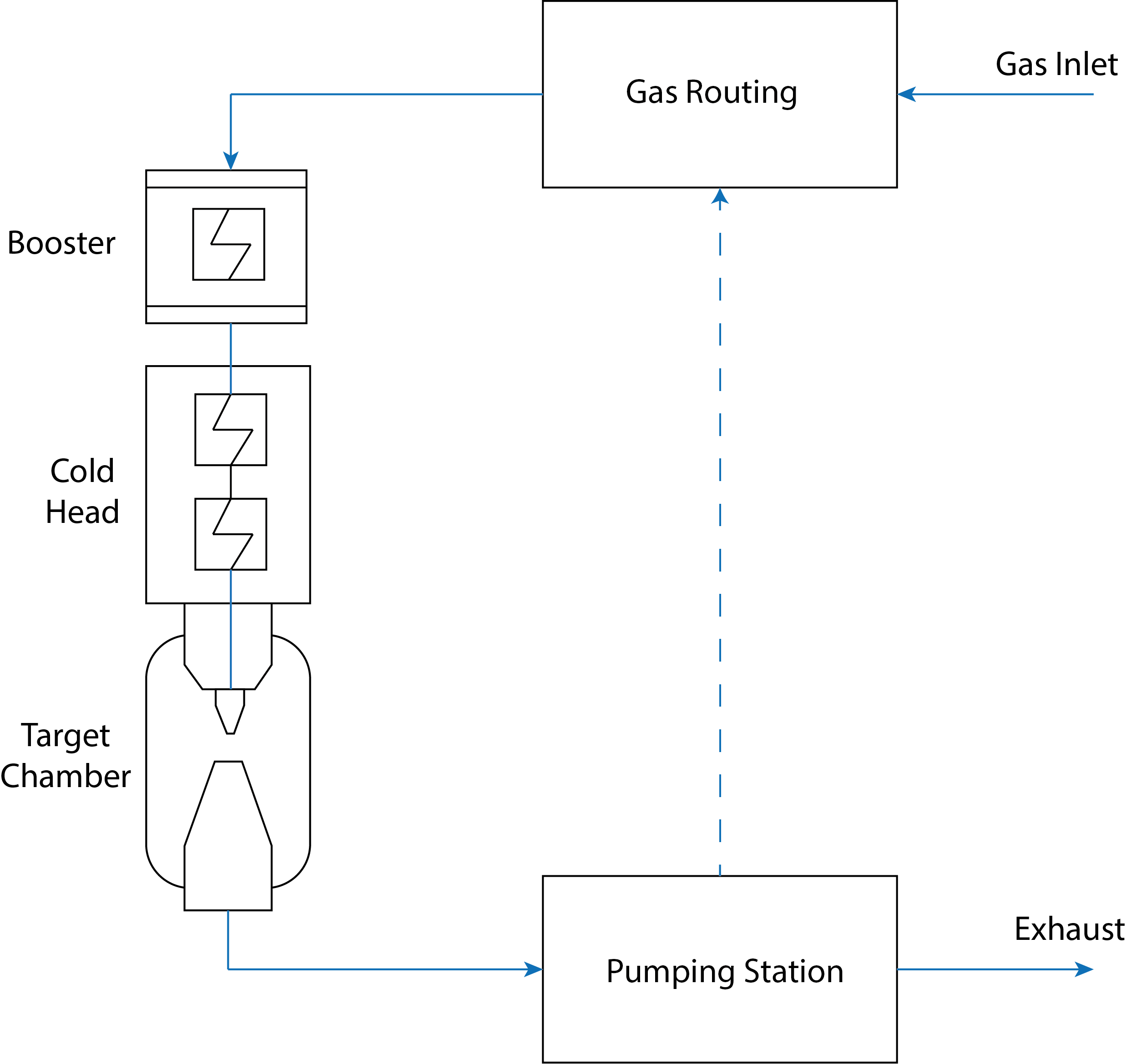
Figure 9: Simplified gas flow diagram of the jet target.

The gas routing system includes mass flow controllers, pressure sensors, temperature sensors, magnetic as well as sampling valves, a hardware state monitor, and a manual interlock button. The entire system is remotely controlled and the measurement of the gas pressure at key positions ensures a high level of control. Sensors which are not delivering a digital signal are included in the system by applying analog to digital conversion. The flow rate of the gas is set in the range between $q_{V}=50\,\mathrm{l_{n}/h}$ and $5000\,\mathrm{l_{n}/h}$ by a Brooks Instrument SLA5851 controller with an accuracy of $\delta q_{V}/q_{V}=$ $\pm$ 0.9 % for a set point between 20 % and 100 % of the full scale and an accuracy of $\delta q_{V}/q_{V}=$ $\pm$ 0.18 % of the full scale below 20 %, corresponding to $\delta q_{V}=\pm 9\,\mathrm{l_{n}/h}$ uncertainty for low flow rates.

To enable the use of rare and expensive target gases, the setup will be extended with a recirculation and purification system.

2.6 Scattering chamber

The aluminum scattering chamber for the gas jet target is depicted in Fig. 10. In order to align the chamber with the beam pipe, a frame underneath allows adjusting the height as well as the tilt. Kapton windows with a height of $120\,\mathrm{mm}$ allow the detection of particles with scattering angles between $\theta=21.5^{\circ}$ and $135^{\circ}$ on the left side of the exit beamline, and between $\theta=11^{\circ}$ and $122.5^{\circ}$ on the right side. Ten universal feedthroughs of different sizes for sensor cables are placed around the chamber. In addition, a glass view port to the pivot point allows the installation of a camera. A DN 260 flange on the side of the chamber is reserved for a turbomolecular pump. A plate on top of the chamber is holding the gas jet target via three fine-threaded bars for a precise adjustment. The tip of the target, confined by a membrane bellow, is lowered into the chamber, see Fig. 11. The catcher can be independently and remotely aligned in all directions, driven by three motorized micrometer screws.

Additional solid state targets are mounted on a rotatable holder which can be moved into the electron beam by a stepper motor: a tungsten wire to determine the width of the electron beam, an aluminum oxide screen to monitor the position of the beam, and a carbon foil for calibration measurements.

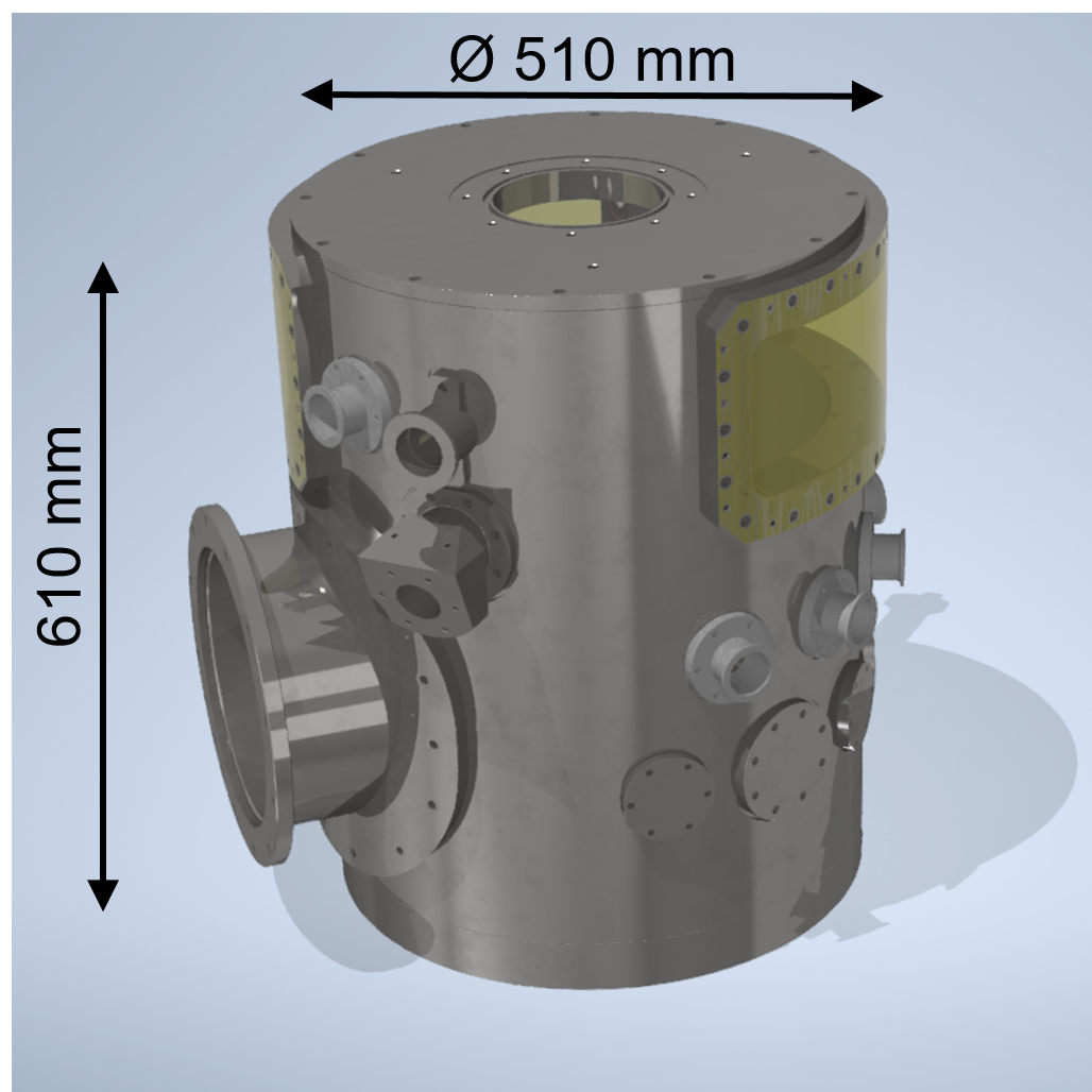
Figure 10: Drawing of the scattering chamber. Kapton windows, several feedthroughs, and the flange for the turbomolecular pump at the left side are visible. To minimize moisture leakage through the windows, an additional layer of aramid foil is placed on top of the Kapton.

Figure 11: Photograph of the inside of the scattering chamber. Target nozzle (top) and catcher (bottom) are located in the center. The beam enters from the right. The catcher can be aligned in all directions, it is attached to the vacuum system by a flexible silicon bellow. Solid state targets are mounted downstream on a holder which can be rotated by a stepper motor. Veto scintillation detectors are placed upstream and can be aligned vertically.

2.7 Vacuum system

To remove the target gas efficiently from the scattering chamber and to keep the residual pressure inside the chamber low, an assembly of pumps is used, see Fig. 12. A set of roots pumps is connected to the catcher: one Leybold RUVAC WH7000FU, one Leybold RUVAC WH2500FU, and one Leybold RUVAC WH700FU. Between the second and the third pump, a gas cooler is installed. The rated pumping speeds, specified for nitrogen, are $S=7000\,\mathrm{m^{3}/h}$, $2500\,\mathrm{m^{3}/h}$, and $710\,\mathrm{m^{3}/h}$, respectively. As roughing pump, a Leybold DRYVAC DV650C screw pump with a rated pumping speed of $S=650\,\mathrm{m^{3}/h}$, is connected. Purge gas can be injected into this pump to allow for a safe operation with oxygen as a target gas. When using hydrogen or helium, no purge gas is used, and a Leybold SCROLLVAC SC30D scroll pump with a rated pumping speed of $S=30\,\mathrm{m^{3}/h}$ is added, because the screw pump is not efficient for light gases. In addition, a Leybold TURBOVAC MAG W2800C turbomolecular pump is directly mounted to the scattering chamber, with a Leybold SCROLLVAC SC15D scroll pump as roughing pump.

Without gas ballast, a pressure of $p\approx 10^{-6}\,\mathrm{mbar}$ is typically reached inside the scattering chamber. Since a significant amount of gas enters the scattering chamber during operation, a larger gas pressure builds up inside. Amongst other things, this results in a reduction of the pumping speed for hydrogen of the turbomolecular pump from $S\approx 2100\,\mathrm{l/s}$ to, for example, $S\approx 180\,\mathrm{l/s}$ at $p=0.2\,\mathrm{mbar}$. Consequences for the applicable gas flow rate are discussed in Subsect. 3.3.

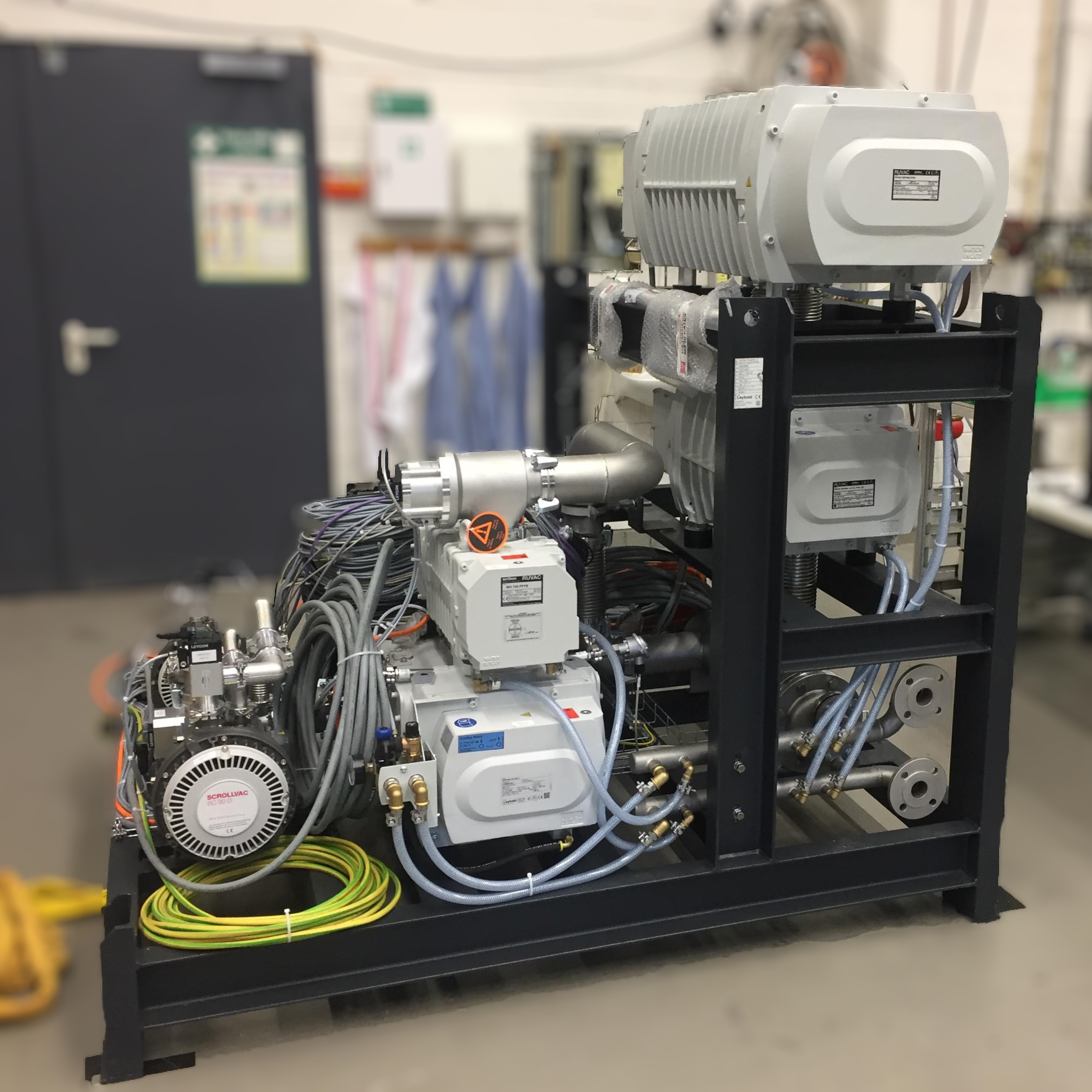
Figure 12: Photograph of the pumping station after its delivery. It consists of three roots pumps, a screw pump, two scroll pumps, a turbomolecular pump (not shown) and a gas cooler. The pumps as well as the valves are controlled remotely. Temperature and pressure sensors provide continuous readout of relevant parameters. Most of the pumps are powered using external frequency converters (not shown). Cooling is mainly performed using a common water cooling circuit.

2.8 Beam halo suppression system

During beam tests with the gas jet target, scattering reactions of electrons from the beam halo with nozzle and catcher were identified. To suppress this kind of background, a collimator and a veto detector were implemented.

2.8.1 Collimator

The upstream collimator consists of two vertically movable absorbers made of tungsten above and below the beam pipe with a thickness of $d=13\,\mathrm{cm}$ along the beam direction. The collimator can block electromagnetic showers of up to $E=1.5\,\mathrm{GeV}$ primary energy. The absorbers are each connected with a shaft to a stepper motor that controls the vertical position, as shown in Fig. 13.

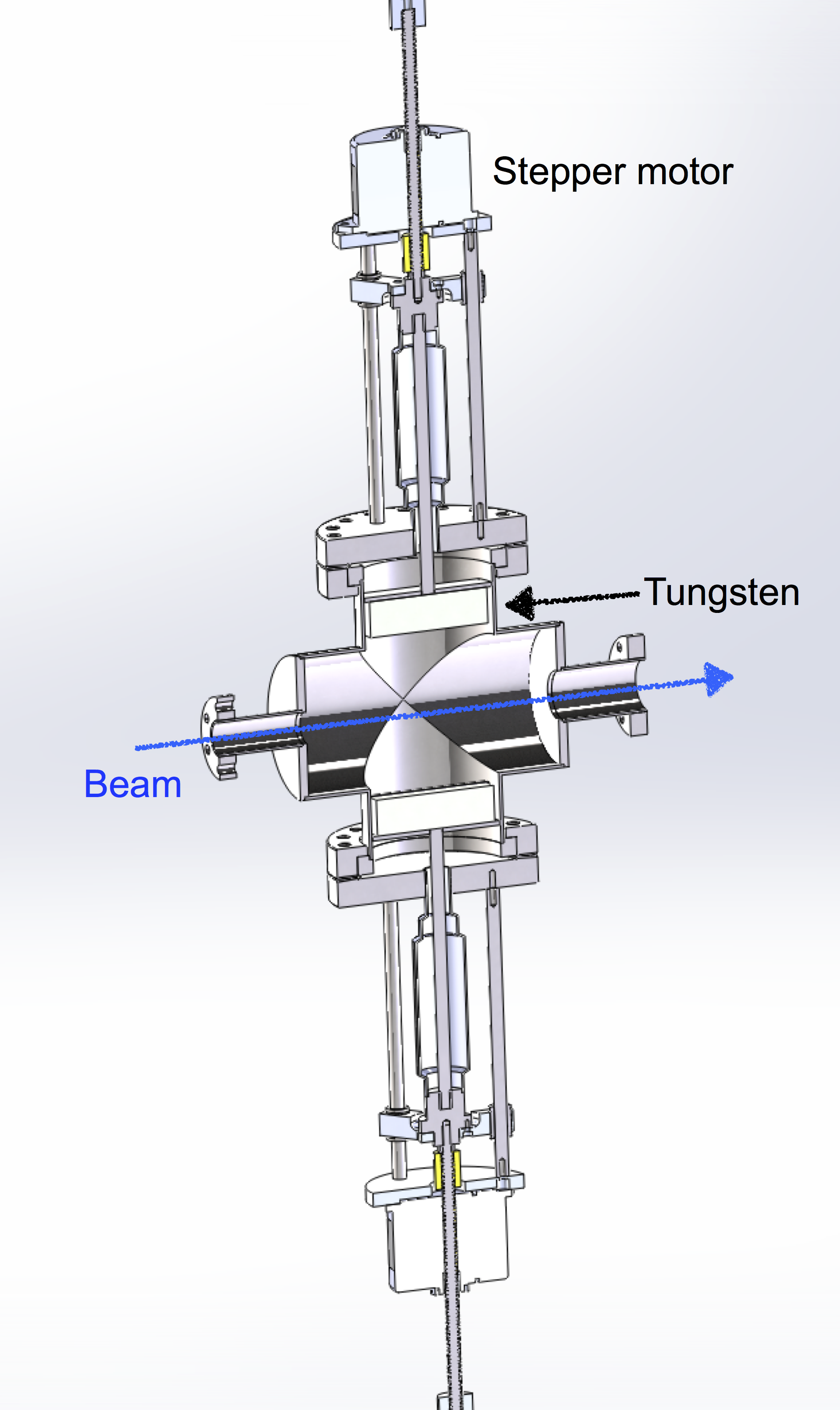
Figure 13: Section view of the collimator assembly. The movable tungsten absorbers are located above and below the beam pipe.

2.8.2 Veto detector

The veto detector is positioned upstream of the gas jet target inside the scattering chamber, as can be seen in Fig. 10. It is designed to reject scattering reactions from residual beam halo electrons hitting the catcher or the nozzle. During the experiment, the positions of the collimator and the veto detectors were adjusted to cover the front of the nozzle and the catcher as much as possible without introducing additional background.

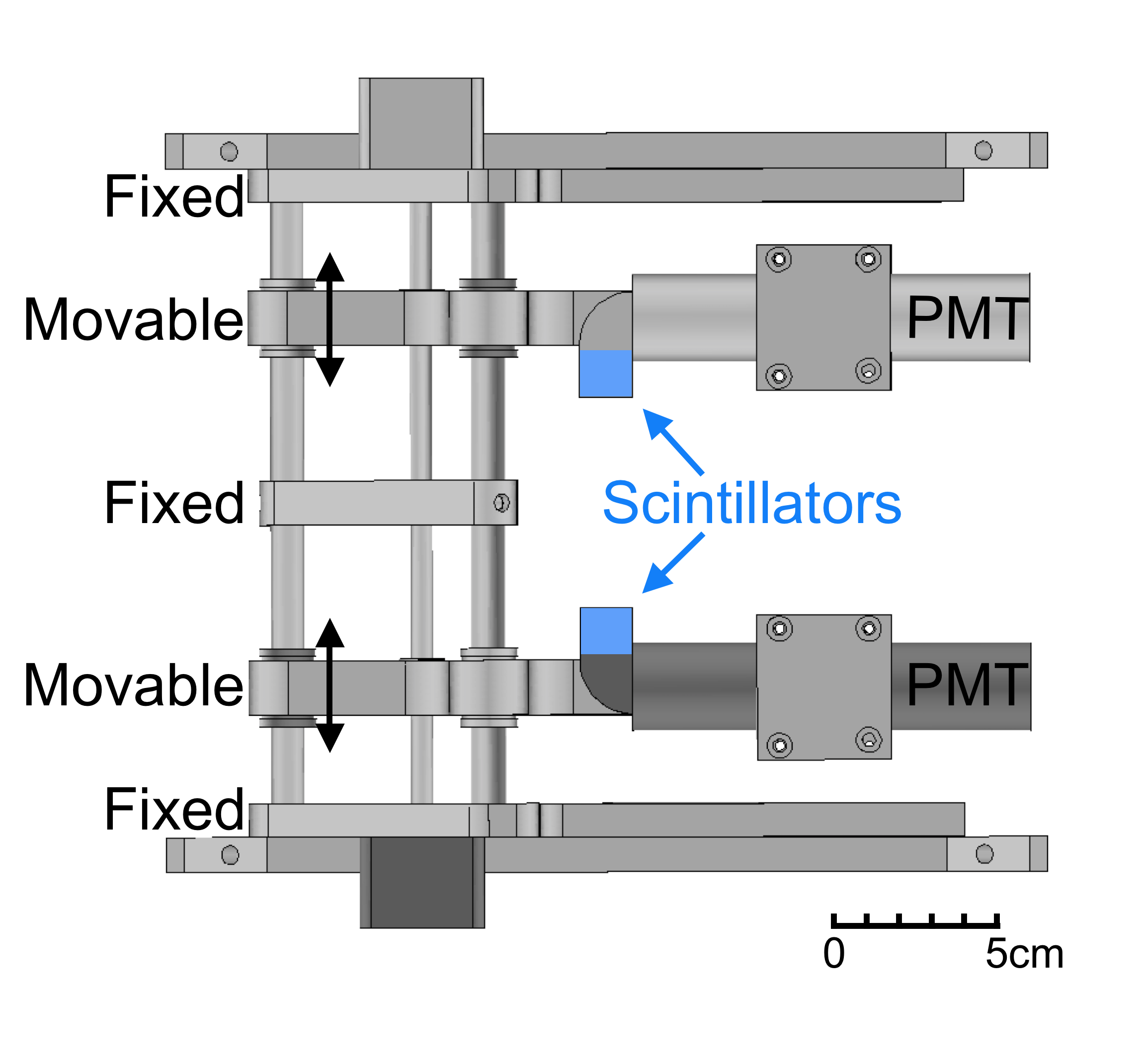
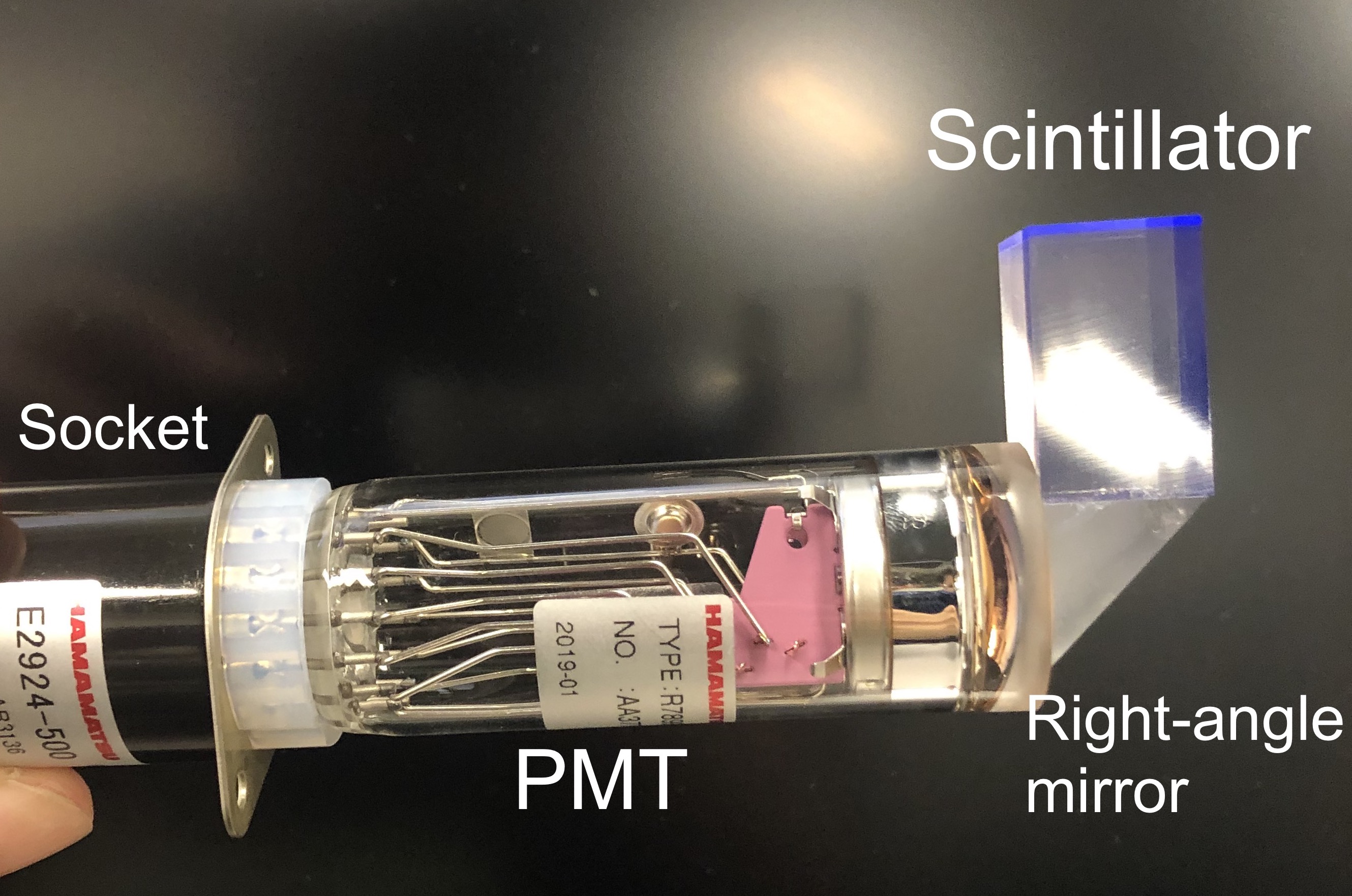
Figure 14: Left: Schematic of the veto system. The beam pipe is located in the center. Right: Photograph of one detector arm with its components.

The detector consists of a frame, a moving mechanism, and the active parts, as shown in Fig 14. The aluminum frame consists of three fixed plates and two moving platforms, one each in a symmetric upper and lower section. The plates are connected by three metal rods. The platforms are guided by three linear shafts along the vertical direction and are moved with stepper motors from Lin Engineering 3518 series. These have 200 steps per revolution, translating to $10\,\mathrm{\mu m}$ per step. One detector arm is mounted on each platform, consisting of a scintillator, a right-angle prism, and a photomultiplier tube (PMT), as shown in Fig. 14. The scintillator is of type EJ-212 from Eljen Technology with dimensions of $15\,\mathrm{mm}\times 15\,\mathrm{mm}\times 20\,\mathrm{mm}$. Its light emission peaks at a wavelength $\lambda\approx$ 430 nm. This light is guided by the prism to the PMT with an efficiency of 99 %. The PMTs are of type R7899 from Hamamatsu with an effective circular area of 22 mm diameter. The PMTs have ten dynode stages and provide a gain of $2.0\times 10^{6}$. Typical rise times are 1.6 ns and pulse lengths are 17 ns.

2.9 Target slow control

The gas jet target setup has 547 controllable parameters in total, requiring a full-scale control system. For this purpose, EPICS (Experimental Physics and Industrial Control System) [29] is used. This is an open source, flexible and scalable system which can be supplemented by modules supplied by the users. For visualization and as graphical user interface, Control System Studio (CSS) is used [30]. CSS is a tool for monitoring and operating large-scale control systems, that is based on the Eclipse source code development system.

Most devices are controlled by separate front-end computers (input-output controllers), currently seven Raspberry Pi with a Debian based Linux system. The communication is mostly achieved by the standard Asynchronous Driver Support (asynDriver4-31) and StreamDevice (V2-6) modules of EPICS [31, 32]. For the controller of the pumping station an additional StreamDevice BUS API is needed to control Profibus devices.

2.10 Analog sensor readout

The analog sensor readout system enables digitizing the output voltages and currents of the analog sensors used in the system. The readout consists of an analog sensor interface, an analog-to-digital converter (ADC), and a Raspberry Pi. The hardware drivers controlling the readout are embedded in EPICS.

The analog sensor interface is a custom-built circuit board that provides a voltage of up to 24 V and enables a channel-wise input configuration by jumpers. The input options are single-ended, differential voltage measurement, or on-board high-precision current-voltage conversion. The output voltage is routed to the ADC board.

The ADC board was custom-built for MESA and MAGIX to share a common hardware platform for slow control and data acquisition. This board provides a relay switch, six digital LVTTL lines, and eight analog differential inputs accepting true negative signals. The analog part is based on two 24-bit delta-sigma analog-to-digital converters of type ADS1248 [33]. The native full-scale input range of $V_{\text{pp}}=\pm$ 2.048 V is expanded using a differential voltage divider to $\pm$ 10 V. The resistors share a common housing and are temperature matched. The input sensitivity can be increased by a programmable-gain amplifier in powers of two within the range between $\times 1$ and $\times 128$. The input channels are sampled during an acquisition time of 50 ms that enables an attenuation of the power grid frequency of ($50\pm 1$) Hz by 66 dB using finite impulse response filters. External parameters, such as supply voltages and the board temperature, are acquired with the maximum sampling frequency of 2 kHz. All values are smoothed with an adjustable moving average filter. The board enables the integration of analog sensors into the EPICS slow control system. With the board’s capability of digitizing voltage as well as current outputs it can be connected to a wide range of different sensors.

3 Operation of the gas jet target

3.1 Alignment of nozzle and catcher

Figure 15: Residual pressure inside the scattering chamber as a function of the horizontal catcher position for a gas flow rate of $1200\,\mathrm{l_{n}/h}$. The optimum position relative to the target nozzle is at the pressure minimum. The $z$ coordinate denotes the direction along the beamline, the $x$ coordinate is perpendicular to it, both have arbitrary offsets.

First, the target nozzle and the catcher were aligned optically at room temperature in a position at the center of the spectrometers using theodolites. It was later observed, that the nozzle tip moved upwards by $\Delta y\approx 2\,\mathrm{mm}$ and horizontally by $\Delta x,\Delta z\approx\nicefrac{{1}}{{4}}\,\mathrm{mm}$ due to thermal contraction during the cooling of the target. Therefore, the warm nozzle had to be aligned in such a way that it moved to the approximate center position during cooling. The remaining vertical offset from the center position could be determined by using the target camera, which simultaneously delivered a centered view of the screen with its scale and the target nozzle. The horizontal offset could be determined using the electron beam during data taking, see Subsect. 4.1. To account for a remaining misalignment of the nozzle to the catcher, the catcher position was adjusted along both horizontal directions with the stepper motors. For its optimum position relative to the target nozzle, a minimum pressure inside the scattering chamber was reached, see Fig. 15. In order to better align the cold target in the future, metal windows with view ports will be attached to the scattering chamber.

3.2 Thermodynamic conditions

During the operation of the gas jet target with hydrogen, the temperature $T_{0}$ is typically chosen to be 40 K and the gas flow rate $q_{V}$ is varied depending on the required areal thickness. The gas pressure $p_{0}$ at the nozzle inlet depends on $T_{0}$ and $q_{V}$ as well as the cross-sectional area $A^{*}$ at the narrowest part of the nozzle. These variables follow the relation [22]

$$q_{V}=A^{*}\frac{p_{0}}{\sqrt{MT_{0}}}\frac{T_{N}}{p_{N}}\left(\frac{2}{\kappa+1}\right)^{\frac{\kappa+1}{2(\kappa-1)}}\sqrt{\kappa R}\,,$$ (2)

with the normal temperature $T_{N}=273.15\,\mathrm{K}$ and pressure $p_{N}=1.01325\,\mathrm{bar}$. For a specific combination of temperature and gas flow rate, the nozzle has to be designed such that on the one hand a sufficient pressure is achieved to form a supersonic jet, and on the other hand the maximum allowable operating pressure of the system is not exceeded. Typical pressures are in the range of $p_{0}=$ 4 bar to 15 bar. When operating the gas jet target, the variables $p_{0}$, $T_{0}$, and $q_{V}$ are measured and their mutual relation can be checked. Differences occur, e.g., when impurities lead to nozzle choking.

When the areal thickness at the nozzle exit is assumed to be homogeneous, it can be estimated by

$$\rho_{\text{areal}}=4N\frac{q_{V}}{\pi dv}\frac{p_{N}N_{A}}{T_{N}R}$$ (3)

from the nozzle outlet diameter $d$, the number of atoms per molecule $N$, the Avogadro constant $N_{A}$, the gas flow rate $q_{V}$ and the gas velocity $v$ as given in Eq. 1. For hydrogen ($N=2$), an areal thickness of $\rho_{\text{areal}}=5\times 10^{18}\,\mathrm{atoms/cm^{2}}$ is reached, when using $d=0.1\,\mathrm{cm}$ and $q_{V}=2400\,\mathrm{l_{n}/h}$ at $T_{0}=40\,\mathrm{K}$. Due to the finite divergence of the gas jet, this value has to be interpreted as an upper limit.

3.3 Gas flow rate during electron beam studies

Figure 16 shows the measured scattering rates for a gas flow rate between $q_{V}=50\,\mathrm{l_{n}/h}$ and $2200\,\mathrm{l_{n}/h}$ during the electron beam studies. While the rate of the reaction of interest, elastic e-p scattering, is proportional to the gas flow rate, the rate of background related events is almost constant up to $q_{V}\approx 1800\,\mathrm{l_{n}/h}$. The nature of the background is studied in detail in Sect. 5. Its major contributions are scattering events of electrons off the nozzle and the catcher. The handling of the data requires a background subtraction, and the related systematic uncertainty scales with the fraction of background to signal events. This makes a high gas flow rate highly desirable. However, with increasing flow rate, the gas pressure increases as seen in the figure.

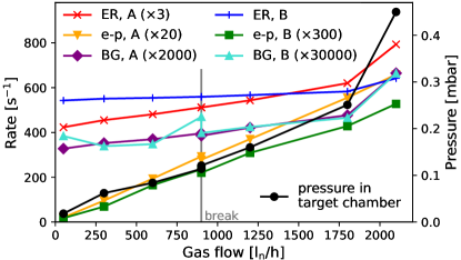
Figure 16: Flow rate-dependent observables during the electron beam study with the hydrogen jet target: Processed event rate (ER) of spectrometers A and B, rate of elastic e-p scattering events as selected by a cut on the missing mass peak region, and rate of background events (BG) from a missing mass sideband analysis. Individual scaling factors have been applied. The pressure inside the target chamber is shown as well. The data points were linearly connected to guide the eye.

The applicable flow rate is limited by the residual pressure inside the scattering chamber. One limiting value is $p\approx 0.5\,\mathrm{mbar}$, the maximum for the attached turbomolecular pump, another is $1\,\mathrm{mbar}$, the maximum for the backflow of target gas into the beamline towards the accelerator. For most of the studies with the electron beam, the gas jet target was operated at $q_{V}=1200\,\mathrm{l_{n}/h}$ without the booster stage and with a residual pressure inside the scattering chamber of $p\approx 0.2\,\mathrm{mbar}$. Optimization of the pumping power as well as the scattering chamber, nozzle and catcher geometries should make it possible to operate the gas jet target at $q_{V}=2400\,\mathrm{l_{n}/h}$ with a lower residual pressure in the future. With the experience gained at the A1 spectrometer setup, the conditions for the MAGIX setup could be extrapolated and a vacuum system with eight smaller pumps was designed, which features a better characteristic at high pressure and will - according to calculations based on the pumping speed curves provided by the manufacturers - allow to improve the residual pressure inside the scattering chamber by one order of magnitude.

4 Characterization of the gas jet

The hydrogen gas jet was studied with a gas flow rate of up to $q_{V}=1500\,\mathrm{l_{n}/h}$. The electron beam was rastered on the target, and the number of elastic scattering events in the spectrometers were measured as a function of the beam displacement. The results are of particular interest for the alignment of the electron beam with the gas jet and for the optimization of the position and the dimension of the catcher. Furthermore, the profile measurements allow to benchmark simulations of the jet properties, and to test target nozzle designs.

4.1 Density profile and horizontal displacement

The measured vertex distribution of scattering events as presented in the upper panel of Fig. 17 is dominated by the wobbler displacement of the beam and exhibits only a small bump in the center. For the data analysis, the vertex displacement, the scattering angle and the missing mass were reconstructed. The missing mass

$$m_{\mathrm{miss}}=\sqrt{(k_{e}-k_{e}^{\prime}+p_{p})^{2}}$$ (4)

with the 4-momenta $k_{e}$ of the incoming electron (given by the beam), $k_{e}^{\prime}$ of the scattered electron (reconstructed by the spectrometer data), and $p_{p}$ of the initial proton (assumed to be at rest), can be reconstructed event-wise for selecting elastic scattering events. For elastic e-p scattering, it peaks at the proton mass $m_{p}$, with radiative effects resulting in a radiative tail at larger values. Scattering events originating at the nozzle exit and the catcher entrance were removed by identifying the elastic e-p scattering events in the missing mass spectrum.

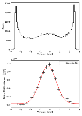
Figure 17: Top: Measured vertex distribution of scattering events. The spectrum is dominated by the wobbler displacement of the electron beam. The small bump in the center is caused by reactions with the gas jet. Bottom: Calculated areal thickness profile showing a clear peak with a Gaussian shape. From a fit to the data, parameters such as peak position, maximum, and width were extracted [34].

For each vertex position, the number of elastic e-p scattering events was determined as a function of the scattering angle and corrected for the spectrometer acceptances from simulations. The luminosity for the measured integrated beam current at each vertex position was then extracted by scaling the count rate to the known cross section [7]. After correcting for the wobbler displacement function, the areal thickness profile was calculated, see the lower panel of Fig. 17. It exhibits a Gaussian shape, from which a constant background contribution ($(0.23\pm 0.01)\cdot 10^{18}\,\mathrm{atoms/cm^{2}}$), which corresponds to the scattering on residual gas inside the scattering chamber, the peak position, the peak maximum ($(0.91\pm 0.03)\cdot 10^{18}\,\mathrm{atoms/cm^{2}}$ above background) as well as the peak width ($\sigma=(0.833\pm 0.024)\,\mathrm{mm}$) were extracted. With a target length acceptance along the beamline of approximately $5\,\mathrm{cm}/\sin(\theta_{\text{B}})=19\,\mathrm{cm}$ for the spectrometer angle $\theta_{\text{B}}=15^{\circ}$ and assuming an axially symmetric gas jet beam, a volume density of $(4.3\pm 0.2)\cdot 10^{18}\,\mathrm{atoms/cm^{3}}$ at the jet center with a background gas density on a $1\cdot 10^{16}\,\mathrm{atoms/cm^{3}}$ level is estimated.

4.2 Gas jet density

Assuming that the gas jet has a two-dimensional Gaussian shape perpendicular to the flow direction, the maximum volume density in the beam center can be expressed by

$$\rho=N\frac{q_{V}}{2\pi\sigma^{2}v}\frac{p_{N}N_{A}}{T_{N}R}$$ (5)

with $N=2$ for hydrogen, the jet width $\sigma$, and the gas velocity $v$ from Eq. 1. Integrating along the direction of the electron beam leads to the maximum areal thickness of

$$\rho_{\text{areal}}=N\frac{q_{V}}{\sqrt{2\pi\sigma^{2}}v}\frac{p_{N}N_{A}}{T_{N}R}\$$ (6)

which provides a better approximation than Eq. 3, but requires the knowledge of the jet width [34]. Assuming a hydrogen flow rate of $q_{V}=2400\,\mathrm{l_{n}/h}$ at a temperature of $T_{0}=40\,\mathrm{K}$ and a typical jet width of $\sigma=1\,\mathrm{mm}$, this results in a maximum volume density of approximately $\rho=6.3\times 10^{18}\,\mathrm{atoms/cm^{3}}$ corresponding to a maximum areal thickness of $\rho_{\text{areal}}=1.6\times 10^{18}\,\mathrm{atoms/cm^{2}}$.

4.3 Gas jet clustering

The divergence of the gas jet, which is also influenced by the onset of clustering formation, has observable effects on the gas pressure as a function of the flow rate. In Fig. 18, this is shown for the residual pressure inside the scattering chamber and the pressure inside the catcher. The change of both of the slopes at $q_{V}\approx 300\,\mathrm{l_{n}/h}$ indicates a more focused gas jet for higher flow rates, so that a larger fraction of it is collected by the catcher. This can be interpreted as a change of state of the gas jet.

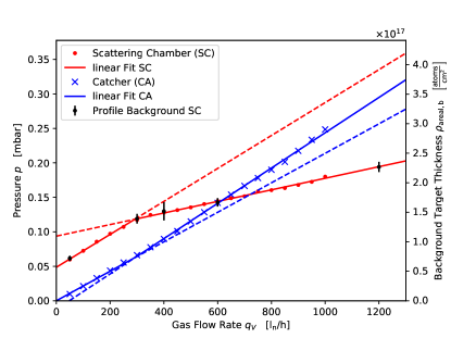
Figure 18: Pressure inside the scattering chamber and the catcher as a function of the hydrogen gas flow rate. The measured background target thickness, which corresponds to e-p scattering not on the gas jet directly but on residual gas inside the scattering chamber, scales with the pressure inside the chamber accordingly. The catcher position was at its optimum, cf. Fig. 15. At a flow rate $q_{V}>300\,\mathrm{l_{n}/h}$ the smaller slope of the pressure inside the chamber and the larger slope inside the catcher indicate a less divergent gas jet.

4.4 Simulation of the gas jet

Numerical simulations were performed to model the expansion of the gas into the scattering chamber [34]. These simulations also allow to optimize the shape of the nozzle outlet which has a large impact on the jet divergence.

The results have been obtained with the solver rhoCentralFoam in OpenFOAM [35]. This solver is able to simulate the compressible, supersonic fluids in a convergent–divergent jet target nozzle, where the speed of sound is reached at the end of the convergent part. Due to conditions close to the phase transition from gas to liquid, the gas properties are modeled with the Peng-Robinson equation-of-state [36]:

$$p=\frac{R_{s}T}{v-b}-\frac{a\,\alpha(T)}{v^{2}+2vb-b^{2}}$$ (7)

with the specific gas constant $R_{s}=R/M$, the specific volume $v=1/\rho$, the constants

$$a=\frac{0.45724\,R_{s}^{2}T_{c}^{2}}{p_{c}}\quad\text{and}\quad b=\frac{0.0778\,R_{s}T_{c}}{p_{c}}$$ (8)

and the function

$$\alpha(T)=\left(1+\lambda\left(1-\sqrt{T/T_{c}}\right)\right)^{2}$$ (9)

with

$$\lambda=0.37464+1.54226\,\omega-0.26992\,\omega^{2}\,.$$ (10)

The values of the state variables depend on the temperature $T_{c}$ and pressure $p_{c}$ at the critical point, and the acentric factor $\omega$, that describes the molecular shape.

The simulations have been performed for six different nozzles geometries with two different designs for the nozzle outlet [34]. All simulated nozzles start with a linearly converging inlet with a half-opening angle of $45^{\circ}$ and a length of 1 mm. The inlet ends with the narrowest inner diameter, which was $d_{\text{min}}=0.5\,\mathrm{mm}$ for the original nozzle used during the electron beam studies in 2018. It is then followed by the outlet with a length of 10 mm, which diverges linearly towards the outlet diameter of $d_{\mathrm{o}}=1\,\mathrm{mm}$. This nozzle type was also simulated with a smaller narrowest inner diameter of $d_{\text{min}}=0.2\,\mathrm{mm}$ and a larger outlet diameter of $d_{\mathrm{o}}=2\,\mathrm{mm}$. In addition to that, a cup-shaped outlet was simulated where the outlet diameter diverges on the first 7 mm and then stays constant for the last 3 mm. Figure 19 shows the two different design types that have been simulated with different diameters.

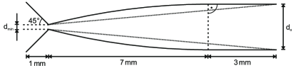
Figure 19: Two different design types of the nozzle outlet considered in the simulations. The linear nozzle outlet, that constantly diverges over the complete outlet length of 10 mm, is drawn with the dotted line. The cup-shaped nozzle is drawn with solid lines. Its outlet forms an arc on the first 7 mm and a constant diameter for the last 3 mm.

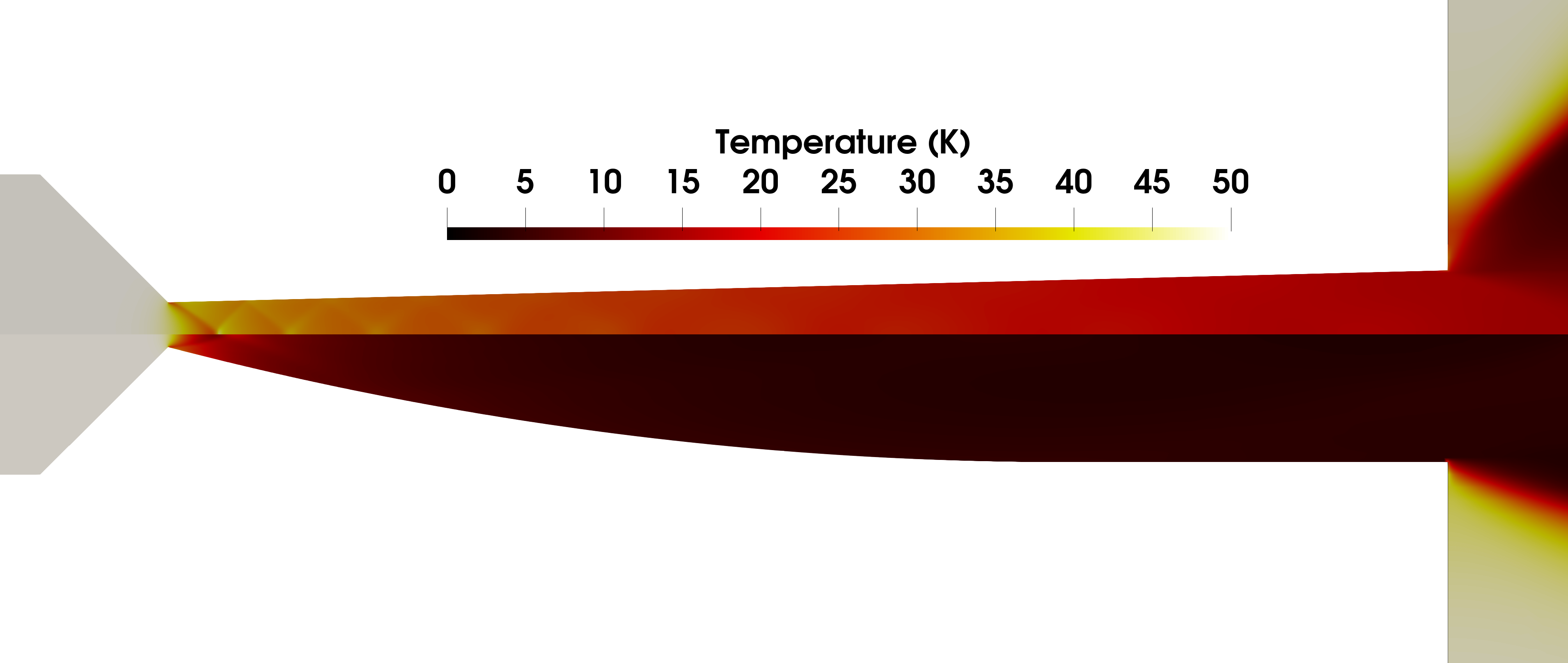
Figure 20: Comparison of the simulated temperature distribution within the linear nozzle with a narrowest inner diameter of $d_{\text{min}}=0.5\,\mathrm{mm}$ and an outlet diameter of $d_{\mathrm{o}}=1\,\mathrm{mm}$ (top) and a cup-shaped nozzle that diverges from $d_{\text{min}}=0.2\,\mathrm{mm}$ to $d_{\mathrm{o}}=2\,\mathrm{mm}$ (bottom). The oscillations at the narrowest inner diameter are typical shock waves for supersonic fluids. On the right a small part of the scattering chamber volume is shown. Both simulations have been performed for a gas flow rate of $q_{V}=1500\,\mathrm{l_{n}/h}$ and an inlet temperature of $T_{0}=50\,\mathrm{K}$ [34].

These simulations show that two effects have a major influence on the target performance. The first one is the dependence of the expansion within the nozzle on the divergence as can be seen in Fig. 20. A greater divergence of the nozzle causes a faster expansion and faster temperature decrease. Secondly, the exact outlet shape is crucial, as the expansion within the cup-shaped nozzles progresses more rapidly as compared to the linear shape. A cup-shaped nozzle with a small $d_{\text{min}}$ and large $d_{\mathrm{o}}$ leads to lower temperatures at the nozzle exit. A small $d_{\text{min}}$ has the additional advantage of a higher pressure that is needed for the same volume flow rate, so that the conditions are closer to the vapor pressure curve. In combination with the lower temperature, this increases the probability for cluster production and thus for a more directed jet.

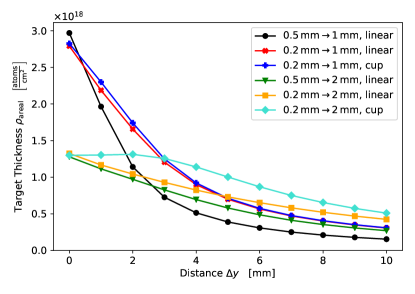
Figure 21: Comparison of the simulated areal thickness for six different nozzle designs as a function of the distance to the nozzle outlet for a gas flow rate of $q_{V}=1500\,\mathrm{l_{n}/h}$ and a temperature of $T_{0}=50\,\mathrm{K}$. Nozzles with a smaller outlet diameter have a larger thickness near the outlet, but exhibit a steeper decrease with distance [34]. The points were interpolated linearly to catch the eye [34].

The simulated areal thickness as a function of the distance to the nozzle outlet for different nozzle designs is summarized in Fig. 21. In agreement with Eq. 3, the thickness for nozzles with smaller $d_{\mathrm{o}}$ is larger directly behind the nozzle, but already at a distance of $\Delta y=3\,\mathrm{mm}$ the cup-shaped nozzle with a larger $d_{\mathrm{o}}$ leads to the largest thickness. This is caused by a smaller divergence due to the faster expansion within the nozzle, so that a compromise in the design has to be found. Since the vertex position is typically in a distance of $\Delta y\approx 4\,\mathrm{mm}$ behind the nozzle outlet, a cup-shaped nozzle was produced and tested with the electron beam.

4.5 Comparison of simulations with experiment

In Fig. 22 the experimentally determined target widths from electron beam studies in 2018 and 2019 are compared to the simulations [34]. In 2018, a linear nozzle with $d_{\text{min}}=0.5\,\mathrm{mm}$ and $d_{\mathrm{o}}=1\,\mathrm{mm}$ was used, in 2019 a cup-shaped nozzle with $d_{\text{min}}=0.2\,\mathrm{mm}$ and $d_{\mathrm{o}}=2\,\mathrm{mm}$. The data are in agreement with the simulations. The cup-shaped nozzle reduces the jet divergence by a factor of two, which leads to twice the areal thickness at the same gas flow rate. With a fit of a linear function to the data, the half-opening angle of the gas jet was extracted. It reduces from $17.2^{\circ}$ to $8.5^{\circ}$ when using the cup-shaped nozzle, although the outlet diameter of this nozzle is larger.

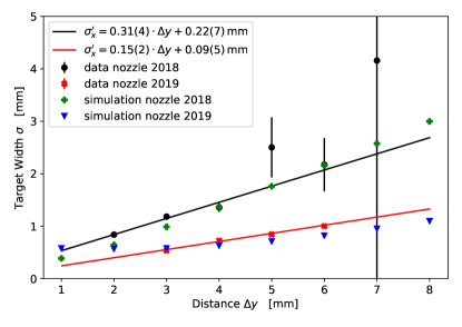
Figure 22: Measured target widths and simulations. The nozzle used in 2018 had a linear shape with $d_{\text{min}}=0.5\,\mathrm{mm}$ and $d_{\mathrm{o}}=1\,\mathrm{mm}$, while the nozzle used in 2019 had a cup shape with $d_{\text{min}}=0.2\,\mathrm{mm}$ and $d_{\mathrm{o}}=2\,\mathrm{mm}$. The experimental conditions were slightly different, in 2018 the target was operated with $q_{V}=1500\,\mathrm{l_{n}/h}$ at $T_{0}=50\,\mathrm{K}$ while in 2019 it was operated with $q_{V}=1200\,\mathrm{l_{n}/h}$ at $T_{0}=40\,\mathrm{K}$. These conditions were considered in the simulations.

5 Background induced by electron beam halo

The areal thickness of the gas jet is much lower than the one of the nozzle and the catcher. In addition, the atomic number is much higher for the nozzle (mainly copper, $Z=29$) and the catcher (aluminum, $Z=13$) than for hydrogen as target gas ($Z=1$). These elements are located a few mm above and below the electron beam, respectively. As a consequence, the presence of an electron beam halo can lead to significant background in scattering experiments, even if the flux of electrons in the halo is many orders of magnitude smaller than in the main core of the beam. Such a halo originates in part from the interaction of the beam electrons with residual gas inside the accelerator, so that it cannot be suppressed completely.

As a countermeasure, a beam halo suppression system was developed, as presented in Subsect. 2.8. The idea behind the multi-step approach was to use the collimator, positioned several meters in front of the target, to absorb a large fraction of beam halo electrons. Since some of them may leak through the collimator or rescatter off the jaws in forward direction, the active shielding at a few cm in front of the target should cover the nozzle and the catcher. In this study, the beam halo veto detector was not used. The focus was the alignment of the collimator system with respect to the target position, which is mandatory in order to achieve minimal, stable, and reproducible background conditions.

5.1 Background introduced by the collimator setup

As the gas jet, when leaving the nozzle, is divergent, the electron beam should be positioned as close as possible to the nozzle to maximize the areal thickness. The positioning of the catcher close to the nozzle is desirable in order to improve the target gas removal. However, if nozzle and catcher are too close to each other, small variations of the beam position would lead to a significant change of the background situation. Shielding the target accurately by means of the collimator becomes more delicate for small relative distances. In conclusion, there is an optimum collimator position for a given distance between the catcher and the nozzle.

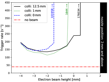
Figure 23: Background event rates of spectrometer B for different positions of the electron beam and the upper collimator, which shadows the target nozzle. When the electron beam position was as close as $\Delta y\approx 1-1.5\,\mathrm{mm}$ to the nozzle or the collimator, the rates increased distinctively.

In an alignment study, scattering rates were measured using the spectrometers without the gas jet for different beam and collimator positions. A minimum distance between the electron beam from the collimator, the nozzle, and catcher of $1.5\,\mathrm{mm}$ was determined, at which no significant background was being produced by the beam hitting these elements, see Figs. 23 and 24.

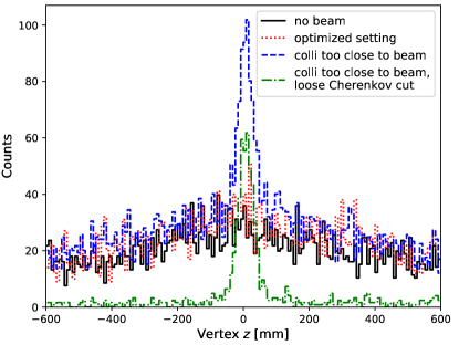
Figure 24: Reconstructed vertex position for selected data, corrected for different run lengths and data acquisition dead times. When the beam position is too close to the collimator, a peak at $z=0$ appears. A signal in the Cherenkov detector identifies these particles as electrons, indicating rescattering of beam halo electrons.

5.2 Background reduction by the collimator setup

Figure 25 shows a missing mass spectrum measured with spectrometer B for different collimator settings. The elastic e-p peak is clearly visible at $0\,\mathrm{MeV}$ and at higher missing mass values its radiative tail is present. Satellite peaks of significant height are located at negative missing mass values, when none of the collimator jaws is used to block the electron beam halo (Out-Out). Moving the lower collimator in (Out-In) shadows the catcher (thin aluminum) from the beam halo and the number of events in the first peak is significantly reduced. Moving the upper collimator in (In-Out) shadows the target nozzle (thick copper) from the beam halo and the second peak is reduced. Moving in both collimators (In-In) reduces the background in both regions.

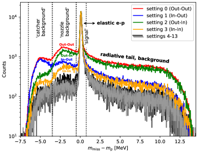
Figure 25: Missing mass spectrum measured with spectrometer B at $\theta_{\text{B}}=15^{\circ}$ and a beam energy of 315 MeV for different collimator settings. The target was operated with $1200\,\mathrm{l_{n}/h}$. The spectra were scaled to the same height of the elastic e-p scattering peak at $0\,\mathrm{MeV}$. The labels for settings 0 to 3 indicate the top and bottom collimator positions, the additional settings correspond to a fine-tuning of the collimator positions which is illustrated in Fig. 26. The missing mass regions of strong backgrounds originating from the catcher and the nozzle are indicated.

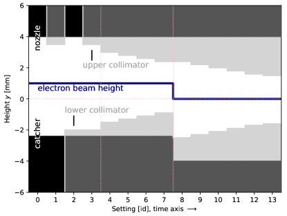
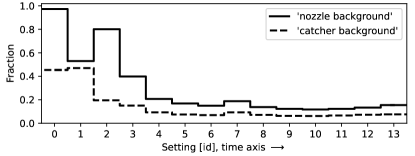
Figure 26: Top: Illustration of different settings during the study of electron beam halo induced background. The height of the nozzle tip relative to the target coordinate system was fixed at 4 mm. The vertical positions of the catcher and the electron beam were changed with setting 8. The positions of the upper and lower collimators were changed in small steps. Bottom: Number of events in the two background regions as defined in Fig. 25 relative to the number of events in the signal region. Setting 13 was used for the subsequent beam studies.

Satellite peaks could be cut from the spectrum in the analysis of e-p scattering. However, their radiative tails and their wide energy loss distributions also contribute to the events in the e-p peak region. Such a background cannot be removed event-by-event, but its distribution needs to be subtracted from the spectrum. As a measure for the blocking effectivity, the number of events in the missing mass regions associated to catcher and nozzle backgrounds were related to the number of events in the elastic e-p region, see Fig. 25. These fractions were evaluated for a number of different collimator settings, which are illustrated in Fig. 26. In addition to the collimator positions, the distance between the catcher and the nozzle was changed once, and the beam position was adjusted accordingly. As it was expected, the background fraction increased when the collimator jaws came too close to the electron beam. For a given distance between the catcher and the nozzle, an optimum position of the collimator could be found.

5.3 Handling of residual background

By inserting the collimators, the background was suppressed by one order of magnitude and a relatively clean e-p scattering spectrum was achieved, see Fig. 27. For a high-precision cross section measurement, i.e., with systematic uncertainties on the sub-percent level, the residual background contribution needs to be determined by additional measurements.

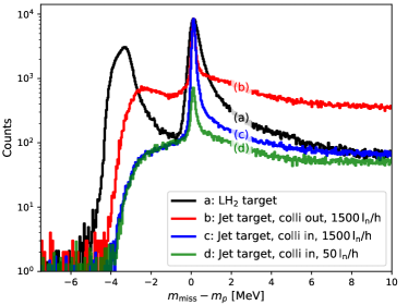
Figure 27: Missing mass spectra for 315 MeV beam energy measured with spectrometer B. The three measurements with the jet target were performed at $\theta_{\text{B}}=15^{\circ}$ without the collimators of the beam halo blocker (colli out), with the collimators inserted corresponding to setting 13 (colli in), and with the collimators inserted and at a reduced gas flow rate. A soft cut on the threshold Cherenkov particle identification detector signal is performed for electron selection. For comparison, a spectrum measured with a liquid hydrogen target cell (black, from [37]) at the same beam energy and similar scattering angles is shown. The gas jet target leads to a narrower peak and has no background from elastic scattering off any cell walls.

A standard background reduction technique for a liquid hydrogen target is the measurement with an empty cell. However, a comparison of the spectra taken with liquid hydrogen and those without provides serious challenges. The electron beam experiences a much smaller energy loss in the empty cell than in the filled one. For example, the mean energy of the electrons, arriving at the backward cell wall, can differ by up to several $\mathrm{MeV}$ with a significantly different energy spread, compare Table 2. Since cross sections depend strongly on the electron energy, measured spectra are shifted and distorted. This is especially problematic as beam-cell interactions produce a large background and its substantial tail contributes to the e-p scattering peak region. Further, the energy spread widens this peak, and a cut on the signal must accept a larger fraction of the background. One solution is to resort to simulations [37]. One advantage of the hydrogen jet target compared to liquid hydrogen targets is that effects from energy loss and multiple scattering do not change significantly when the gas flow rate is changed. When using the gas jet target, a measurement without any gas flow is obviously ideal to provide a pure background measurement. In the presented study, a warm target system was avoided because of the thermal movements that result in a different background situation, and measurements were taken at cryogenic temperatures with a finite gas flow rate of $q_{V}=50\,\mathrm{l_{n}/h}$ to minimize the risk of a freezing nozzle in the case of any undetected vacuum leaks. At MAGIX, a precise adjustment of the target position will be possible during operation to accomodate any movements and measurements will be performed without any gas flow. The resulting spectrum in Fig. 27 demonstrates that the rate of elastic e-p events is significantly reduced, while the rate from interactions of beam halo electrons with the target structure, which dominates the spectrum outside the elastic peak region, remains unchanged. Although the gas flow rate is reduced by a factor of 30, the number of counts in the elastic peak is reduced by a factor of approximately 12 only. The reason why this factor is lower can be explained by the fact that no cut on the vertex position has been applied, avoiding possible distortions of the spectra, and the event yield associated with a scattering on the residual gas does not decrease linearly with the gas flow, compare Fig. 18. The result for this factor agrees well with the expectation based on an evaluation of data dedicated to the density profile measurements, $12.2\pm 1.5$. This spectrum can be used to model the background or to subtract it. For comparison, the missing mass peak from a measurement with a liquid hydrogen target is shown in Fig. 27 as well.

6 Stability of the luminosity

A sub-percent measurement of the luminosity $\mathcal{L}$, proportional to beam current and areal thickness of the gas jet, is crucial for high-precision experiments. While different techniques can be used for the determination of the absolute value of the beam current, the areal thickness of the gas jet can not be inferred from the measured target parameters with high accuracy. In addition, a small change in the horizontal beam position of $\Delta x\approx$ $\pm$ 0.2 mm can result in a significant change of the luminosity by $\Delta{\mathcal{L}}\approx$ $\pm$ 2 % due to the varying overlap of the beam with the jet.

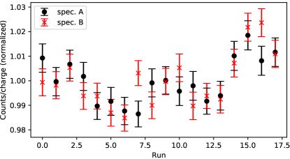
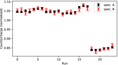
Figure 28: Top: Normalized event rates per run measured with spectrometer A and B for the setting with B at a scattering angle of $\theta_{\text{B}}=20^{\circ}$. A correlated drift of the rates is observable. Bottom: Normalized event rates per run measured with spectrometer A and B for the setting in which the gas flow rate of the jet target was reduced by approximately 20 % after run 17. Both event rates follow the change in luminosity.

A simultaneous measurement of the Møller scattering cross section could provide a relative luminosity determination. Alternatively, if more than one high-resolution magnetic spectrometer is available in the experimental setup, one of them could be used at a fixed setting for elastic e-p scattering. The achievable accuracy is limited by the knowledge of the reference cross section. Moreover, for experiments such as elastic form factor measurements, the data analysis can be performed using a floating normalization, where physical constraints are used to adjust common normalization parameters, see Refs. [7, 37].

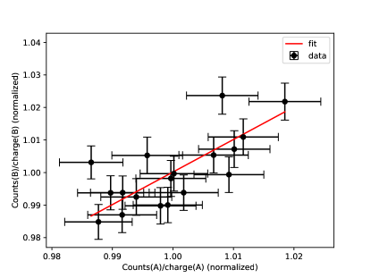
Figure 29: Correlation of the normalized event rates per run for the setting with spectrometer B at a scattering angle of $\theta_{\text{B}}=20^{\circ}$. A linear fit through the origin was applied.

For different angular settings of the spectrometers, multiple runs with a length of 30 min each were taken over a period of several days to study the stability of the luminosity and to test the reliability of the relative luminosity monitoring. The number of events in the elastic e-p scattering peak for each run was extracted for both spectrometers by subtracting the background, correcting for the measured data acquisition dead time, and applying a missing mass cut at $-0.5\,\mathrm{MeV}<m_{\text{miss}}-m_{p}<2\,\mathrm{MeV}$. This number was normalized by the integrated charge from the beam current measurement using a Förster probe. Figure 28 gives an example for a setting with spectrometer B at a scattering angle of $\theta_{\text{B}}=20^{\circ}$. A drift of the event rates per run beyond statistical fluctuations was observed in both spectrometers. Figure 29 demonstrates a linear correlation caused by luminosity drifts. The root mean square value $\text{RMS}_{\text{A/B}}\approx 0.0087$ of the distribution of the count rate ratio from spectrometers A and B agrees well with the typical statistical uncertainty $\sigma_{\text{A/B}}^{\text{typ}}\approx 0.0090$ of a single run. In one setting the gas flow rate of the jet target was intentionally reduced by about 20 %, see Fig. 28. The mean value of the ratio for the runs with a higher gas flow, 0.3312 $\pm$ 0.0030 , does not deviate from the mean value for the runs with the lower gas flow, 0.3314 $\pm$ 0.0036 . The values for all settings in this study are tabulated in Table 1. A very important result is that no sign of a significant systematic error contribution exceeding the statistical uncertainty was found. One can conclude that drifts of the luminosity that could be on a scale of 10 % over several days can be measured precisely by using one spectrometer as a luminosity monitor.

Table 1: Luminosity study with different settings. Spectrometer A was fixed at a scattering angle of $\theta_{\text{A}}=30^{\circ}$, while the scattering angle $\theta_{\text{B}}$ of spectrometer B was varied. For each setting $\#$ denotes the number of runs per setting, $D_{A}=(\text{max}-\text{min})/\text{mean}$ is the range of deviations of the event rate measured with spectrometer A, $\sigma_{\text{A/B}}^{\text{typ}}$ is the typical statistical uncertainty of the ratio of the event rates measured by the two spectrometers in a single run, and $\text{RMS}_{\text{A/B}}$ is the root mean square of its distribution.

$\theta_{\text{B}}$	$\#$	$D_{A}$	$\sigma_{\text{A/B}}^{\text{typ}}$	$\text{RMS}_{\text{A/B}}$
20∘	18	0.032	0.00903	0.00868
25∘	47	0.059	0.00205	0.00217
30∘	73	0.101	0.00134	0.00128
35∘	82	0.060	0.00113	0.00143
40∘	82	0.172	0.00161	0.00134

7 Comparison to other hydrogen targets

Table 2: Typical parameters of the hydrogen jet target for MAGIX compared to other hydrogen targets in current nuclear physics experiments at electron accelerators. State denotes the state of hydrogen inside the target, setup refers to the experiment or setup, $T_{0}$ is the operating temperature, $l$ the length in beam direction, $\rho_{\text{areal}}$ the areal thickness, $I_{\text{beam}}$ the maximum beam current achievable for the setup, $\mathcal{L}$ the maximum achievable luminosity, $E_{\text{beam}}$ the typical beam energy, and $\Delta E_{\text{beam}}$ the most probable energy loss for electrons at the typical beam energy. The last two columns address the background in terms of cell walls and hydrogen purity. The beam energy loss is calculated employing the energy-dependent total stopping power from Ref. [38] for a full passage of the target including target cell walls at the front and back where in use. The impinging electron beam is assumed to be centered and point-like. The FWHM spread of the energy loss is not separately listed: According to Landau theory, it is of the order of 11 %. Note that the OLYMPUS and the DarkLight targets have side walls, and the PRad target a Kapton foil which scattered electrons have to pass in addition.

State	Setup	$T_{0}$	$l$	$\rho_{\text{areal}}$	$I_{\text{beam}}$	$\mathcal{L}$	$E_{\text{beam}}$	$\Delta E_{\text{beam}}$	Windowless	Purity
		[K]	[mm]	[$10^{18}\,\mathrm{\frac{atoms}{cm^{2}}}$]	[$\mu$A]	[$10^{35}\,\mathrm{cm^{-2}s^{-1}}$]	[MeV]	[keV]
gas	gas jet, A1	$40$	$\sigma\approx 1$	$1$	$20$	$0.001$	$195$	$0.01$	✓	✓
gas	gas jet, MAGIX	$40$	$\sigma\approx 1$	$2$	$1000-10000$	$0.1-1$	$105$	$0.02$	✓	✓
gas	PRad	$25$	$40$	$2$	$0.01$	$0.00001$	$2200$	$0.13$	(✓)	✓
gas	DarkLight	$293$	$600$	$1.2-10$	$10000$	$0.7-6$	$100$	$0.01-0.11$	(✓)	✓
gas	OLYMPUS	$75$	$600$	$0.003$	$65000$	$0.01$	$2000$	$0.0002$	(✓)	✓
liquid	round LH2, A1	$23$	$20$	$84000$	$10$	$52$	$195$	$1245$	$\times$	✓
liquid	cigar LH2, A1	$23$	$50$	$210000$	$10$	$131$	$195$	$2944$	$\times$	✓
liquid	LH2, MUSE	$21$	$60$	$251000$	$0.0000005$	$0.000008$	$160$	$3345$	$\times$	✓
liquid	waterfall, A1	$293$	$0.5$	$3600$	$20$	$4$	$195$	$388$	✓	$\times$
solid	plastic, A1	$293$	$2$	$16000$	$1$	$1$	$195$	$1200$	✓	$\times$

A comparison of the main parameters of hydrogen targets used in current nuclear physics experiments at electron accelerators such as Darklight [39], OLYMPUS [40, 41], PRad [42, 43], MUSE [44, 45], and A1 at MAMI [37, 46, 47, 48, 49] is given in Table 2, an overview of previous targets can be found in [50].

Liquid hydrogen targets are common. Inside a containing target cell of several cm length, a sizable amount of hydrogen is provided at cryogenic temperatures. On the one hand, the large areal thickness allows to reach high luminosities, on the other hand, incoming electrons as well as outgoing particles can be significantly affected by the large thickness. An absolute areal density determination on the percent-level is feasible for such targets by knowledge of the cell geometry and monitoring the target parameters while taking care that the beam load does not substantially change the density of the hydrogen by local heating above the boiling point. However, the target cell material itself, e.g., a metal or metal alloy, and additional layers of superinsulation foil can be a significant source of irreducible background. Empty cell measurements need to be acquired for background subtraction.

Liquid or solid state targets consisting of a compound material including hydrogen, such as waterfalls (H₂O) or plastics (CH₂), can be constructed without any walls. The impurities in the form of nuclei other than hydrogen lead to irreducible background contributions. In turn, these can be used for a relative cross section measurement, for instance, normalizing the e-p cross section to the e-¹²C cross sections, and vice versa. The absolute areal density can in principle be determined on a percent-level as well, with limitations arising from the determination of the target length in beam direction or the knowledge of the target volume density. In case of solid state targets such as plastics, a change of chemical or physical properties during the experiment could be an issue. For instance, a physical deformation of the target shape or a variation of the ratio of hydrogen to other atoms is possible when the target is heated by the electron beam.

Basic features of gas targets are a small areal thickness, a high purity, and the possibility for a windowless design. As a result, very clean data can be obtained, with negligible effects from energy straggling and multiple scattering, and a minimum of irreducible background related to target contamination and cell walls. Because of the small areal thickness, high beam currents must be provided to achieve competitive luminosities. In this aspect, a windowless design avoids the destructive heating of cell walls and allows for the recirculation of the beam inside a storage ring or an energy recovery linac. None of the gas targets listed in Table 2 have a window along the beam line. The OLYMPUS and the DarkLight targets have side walls, which the scattered electrons have to pass before detection. In the PRad setup, holes inside Kapton foils allow the beam to enter and exit the hydrogen gas volume without producing background. Based upon our understanding, all scattered electrons except those at the smallest angles have to pass this foil.

For high-precision experiments, it is important to correct for the most probable energy loss of the incoming electron as well as of the outgoing electron and other particles to improve the momentum determination. A reconstruction of the vertex point increases the accuracy, since the energy loss depends on the path length in the target material. For a precise comparison of measurements to simulations, the distributions of energy loss, external bremsstrahlung and multiple scattering need to be modeled. It is evident that windowless gas targets provide the highest precision.

8 Summary and outlook

In this paper, the performance of a new cryogenic gas jet target in an electron accelerator experiment was presented. The target was designed to be the centerpiece of the upcoming MAGIX electron scattering setup at the MESA energy recovery linac. Its windowless design facilitates a new level of precision. Previous setups have been limited by systematic effects associated with energy straggling, multiple scattering, and irreducible backgrounds.

The target was successfully commissioned at the spectrometer setup of the A1 Collaboration at MAMI, and its performance was studied. The size of the gas jet is small, $\sigma\approx 1\,\mathrm{mm}$, which is ideal for use at high-resolution spectrometer setups, and its areal thickness, $\rho_{\text{areal}}\geq 10^{18}\,\mathrm{atoms/cm^{2}}$, is small enough for beam recirculation, but large enough to provide competitive luminosities of up to $\mathcal{L}\approx 10^{35}\,\mathrm{cm^{-2}s^{-1}}$ with the high beam currents anticipated at MESA.

A severe issue was found related to the electron beam halo, which can scatter off parts of the target assembly and produce significant background contributions. As a solution, a beam halo blocker was installed, which successfully reduced this background by one order of magnitude. From measurements with different gas flow rates, the residual background contribution was determined and a precise background subtraction was performed.

Although the main motivation of the target installation at MAMI was a test of the target system under experimental conditions, high-quality e-p scattering data have been collected. Figure 30 shows the online analysis of the e-p cross section from the first commissioning beam time.

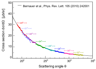
Figure 30: Cross section measurement of elastic e-p scattering during commissioning of the gas jet target compared to the data from Ref. [7]. The data were collected using eight different angular and magnetic field settings of spectrometer B with one common normalization parameter. The central spectrometer angle for each of the settings is depicted in the figure. Spectrometer A provided a monitoring of the luminosity.

The setup and data quality have improved significantly since then, and settings dedicated to a precise proton form factor measurement have been determined and the collected data are currently under analysis.

In the future, the consistent windowless design of the MAGIX target will enable the detection of low-energy recoil particles such as protons, deuterons, or $\alpha$-particles in detectors inside the scattering chamber. Measurements with argon as target gas are planned in the near future. The finalization of a gas recirculation will further enable the use of expensive gases such as deuterium and helium, while the use of oxygen is challenging but highly desirable to study the ¹⁶O$(e,e^{\prime}\alpha)^{12}$C reaction. The possibility to use many different gases makes the jet target ideal for the versatile physics program with the MAGIX setup at MESA, which will come into operation in a few years.

redThese appendices are not included in the submitted version.

Appendix A Background subtraction

A.1 Example spectra

Data for the elastic e-p cross section determination were taken with a high gas flow rate of $q_{V}=1200\,\mathrm{l_{n}/h}$. Additional data were taken with a low gas flow rate of $q_{V}=50\,\mathrm{l_{n}/h}$ and without beam for background subtraction, see Fig. 31 (a).

The approximate shape of the background was deduced from the low flow spectrum which includes a small elastic e-p peak on top of the background. From this data the high flow spectrum was subtracted after appropriate scaling, see Fig. 31 (b). In addition to beam related background, also cosmogenic background contributes to the spectrum, its fraction varies for instance with the beam current and with the data acquisition dead time. To accommodate, we include data measured without beam to the background model. In Fig. 31 (c), the beam related background spectrum and the cosmogenic background spectrum were scaled and summed to match the high flow data in the background region of the spectrum. The background free spectrum was obtained from the high flow data by subtraction of the full background contribution. A sharp elastic e-p scattering peak with radiative tail remains, see Fig. 31 (d).

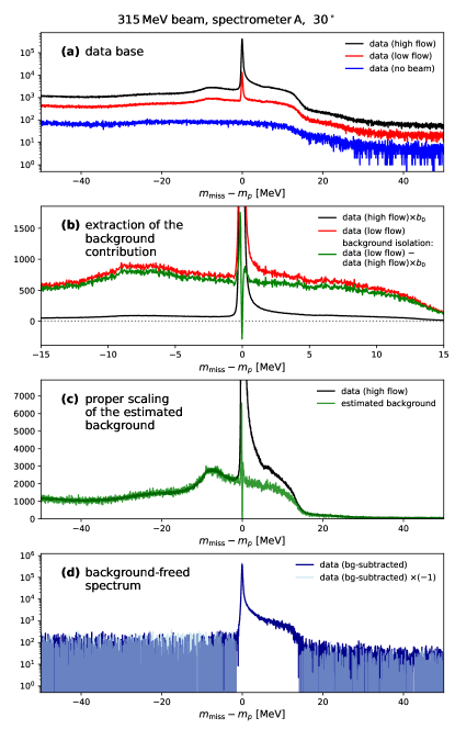
Figure 31: Missing mass spectra taken for elastic e-p form factor measurements. (a) Measured counts in the individual data sets. (b) Extraction of the beam related background spectrum. (c) Full background spectrum including beam related and cosmogenic background. (d) Background subtracted elastic e-p scattering spectrum. The inverted spectrum is shown in addition to visualize the scattering around zero aside the elastic peak in the logarithmic scale.

A.2 Error contribution related to background subtraction

To control target-related uncertainties at a sub-percent level, measurements at a high gas flow rate must be accompanied by an appropriate amount of data taken at a low gas flow rate. To estimate the best fraction of high to low flow settings for a minimal uncertainty, one assumes a constant beam current, constant detector and data acquisition dead times, a pure background spectrum in the low flow spectrum, and no cosmogenic background. Furthermore, all event counts are assumed to be large so that the statistical uncertainty can be estimated by the square root of the event count.

With $\dot{S}_{\text{high}}$ as the expected rate of signal events measured in a high flow setting, the number of expected signal events within a measurement time of $t_{\text{high}}$ is $S_{\text{high}}=S_{\text{high}}(t_{\text{high}})=\dot{S}_{\text{high}}\cdot t_{\text{high}}$ with a statistical uncertainty of

$$\Delta S_{\text{high}}=\sqrt{S_{\text{high}}}.$$ (11)

If the fraction of background to signal events is $b_{\text{high}}$ in the high flow setting, a number of $B_{\text{high}}=\dot{B}_{\text{high}}\cdot t_{\text{high}}=b_{\text{high}}\cdot S_{\text{high}}$ background events is expected in the very same measurement. The low flow setting provides the estimate $B_{\text{high}}^{\text{est.}}$. This requires either a precisely monitored beam current, so that the scale between the low flow and the high flow setting is well known, or a precise scaling by comparison of the background dominated part of the spectra. The background subtracted number of signal events $S_{\text{high}}^{\text{bgs}}$ is:

$$S_{\text{high}}^{\text{bgs}}\approx\underbrace{S_{\text{high}}+B_{\text{high}}}_{\text{high\ flow\ settings}}-\underbrace{B_{\text{high}}^{\text{est.}}}_{\text{low\ flow\ settings}}.$$ (12)

Accordingly, the uncertainty of the estimate

$$B_{\text{high}}^{\text{est.}}=B_{\text{low}}(t_{\text{low}})\cdot\frac{t_{\text{high}}}{t_{\text{low}}}$$ (13)

contributes to the total error. It is related to the statistical precision of $B_{\text{low}}$. In addition, $B_{\text{high}}$ contributes the statistical uncertainty

$$\Delta B_{\text{high}}=\sqrt{b_{\text{high}}\cdot S_{\text{high}}},$$ (14)

which can not be reduced by supplemental background measurements.

If for an available measurement time $t_{\text{total}}=t_{\text{high}}+t_{\text{low}}$ the same amount of time is used for the different gas flow settings, the two contributions of the background error are equal,

$$\Delta B_{\text{high}}^{\text{est.}}\approx\Delta B_{\text{high}},\quad\textnormal{for }t_{\text{high}}=t_{\text{low}}.$$ (15)

The minimal error for $S_{\text{high}}^{\text{bgs}}$, however, can be achieved for a value of

$$r=\frac{t_{\text{low}}}{t_{\text{high}}},$$ (16)

which depends on the background to signal ratio $b_{\text{high}}$. If, for instance, the background contribution is negligible, a smaller $r$ will provide a smaller total error. In the hypothetical case of a background-free measurement, one could use all available time for the high flow setting. With this special case as a reference,

$$S_{0}=S_{\text{high}}(t=t_{\text{total}}),\quad\Delta S_{0}=\sqrt{S_{0}},$$ (17)

and using

$$t_{\text{low}}=t_{\text{total}}\cdot\frac{1}{1+1/r},\quad t_{\text{high}}=t_{\text{total}}\cdot\frac{1}{1+r},$$ (18)

it follows:

$$\frac{\Delta S_{\text{high}}^{\text{bgs}}}{S_{\text{high}}^{\text{bgs}}}(r)\approx\frac{\Delta S_{\text{high}}^{\text{bgs}}(r)}{S_{\text{high}}(t_{\text{high}})}$$

$$\quad\approx\frac{\sqrt{(\Delta S_{\text{high}}(t_{\text{high}}))^{2}+(\Delta B_{\text{high}}(t_{\text{high}}))^{2}+(\Delta B_{\text{low}}(t_{\text{low}})/r)^{2}}}{S_{0}\cdot\frac{t_{\text{high}}}{t_{\text{total}}}}$$

$$\quad=\frac{\sqrt{\Delta S_{0}^{2}\cdot\frac{1}{1+r}+\Delta S_{0}^{2}\cdot\frac{1}{1+r}\cdot b_{\text{high}}+\Delta S_{0}^{2}\cdot\frac{1}{1+1/r}\cdot\frac{1}{r^{2}}\cdot b_{\text{high}}}}{S_{0}\cdot\frac{1}{1+r}}$$

$$\quad=\frac{\Delta S_{0}}{S_{0}}\cdot\sqrt{1+2b_{\text{high}}+r(1+b_{\text{high}})+b_{\text{high}}/r}$$ (19)

The relative error with respect to the relative error for a background-free measurement is shown in Fig. 32 as a function of $r$ for different background fractions $b_{\text{high}}$. It is minimized at an optimal data taking ratio of

$$r_{\text{opt}}=\sqrt{\frac{b_{\text{high}}}{1+b_{\text{high}}}}.$$ (20)

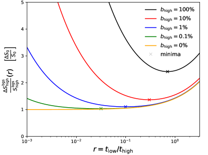
Figure 32: The relative uncertainty of the signal as a function of the fraction of time spent for measuring at high and low flow settings shown for different background to signal fractions $b_{\text{high}}=B_{\text{high}}/S_{\text{high}}$ in the high flow data.

Fig. 33 shows $r_{\text{opt}}$ as a function of $b_{\text{high}}$ as well as the relative error of the measurement signal after background subtraction for the optimal $r_{\text{opt}}$.

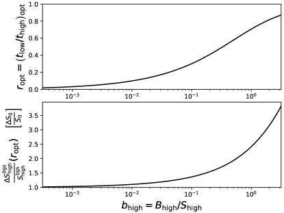
Figure 33: Top: Optimal ratio of measurement times for the low and high flow settings. Bottom: Relative error with respect to the hypothetical error for a background free measurement during the available time $t_{\text{total}}$.

For the data presented in Fig. 31 with a cut on the Cherenkov detector signals to remove the cosmogenic background and a cut on the missing mass region from $-2\,\mathrm{MeV}$ to $15\,\mathrm{MeV}$ to select the elastic e-p scattering peak, the fraction of background events below the elastic peak is 6.7 %. From the previous considerations follows $r_{\text{opt}}=25\,\mathrm{\%}$, i.e., the time spent for the low flow setting with respect to the high flow setting should be $1:4$ in order to achieve a minimal error.

Appendix B Nitrogen level meter of the booster stage

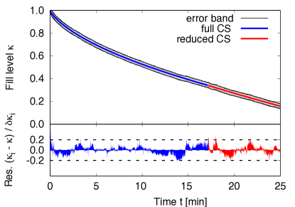
Figure 34: Typical time evolution of the liquid nitrogen (LN) fill level after automated refill. Upper panel: The evaporation of LN for precooling of the target gas evolves linearly in time. The cooling of the initially warmed dewar causes an additional LN consumption following an exponential law. Below a fill level of $\kappa=34\,\mathrm{\%}$, the heat exchanger is mounted which reduces the effective cross section (CS) of the LN volume. This results in a faster decrease of the level when assuming a constant evaporation per unit volume. Lower panel: The residual $\kappa_{i}-\kappa$ of a single measurement $i$ is below 20 % of the Poisson distributed counting error $\delta\kappa_{i}$.

The nitrogen level meter monitors the fill level of the booster stage and enables an automated refill during operation of the gas jet target. It consists of two concentric stainless steel tubes forming a cylindrical capacitor by enclosing a sensitive volume in the interspace. Liquid nitrogen in the sensitive volume modifies the dielectric, since its relative permittivity $\epsilon=1.425$ [51] is larger than that of gaseous nitrogen $\epsilon\approx 1$. The sensitive volume can be reached by the liquid only through small holes at the bottom. These holes are acting as a flow impedance that limits the hydrodynamic coupling to fluctuations during the refill process. The pressure inside the sensitive volume is equalized through an opening at the top, that is shielded by amorphous SiO₂ against moisture.

The meter capacitance is converted to an equivalent frequency by an oscillator circuit, that cyclically charges and discharges the cylindrical capacitor through a resistor. A symmetric oscillator with a precision reference capacitor is thermally coupled to the main oscillator. Both frequencies are measured by fast synchronized 32 bit-counters with an adjustable acquisition time. The fill level is determined from the ratio of both counters, in which the dependence on the acquisition time cancels and the dependence on oscillator specific parameters is weak.

The statistical accuracy is optimized by oscillator frequencies in the MHz range, low-capacitance connection cables, and signal filtering with an adaptive-sized moving average. In combination with the flow impedance as an hydrodynamic low pass filter, this results in an excellent fill level resolution, see Fig. 34. The hardware drivers are running on a Raspberry Pi and are interlinked with the EPICS database, c.f. Subsect. 2.9.

References

- [1] J. D. Walecka, Electron scattering for nuclear and nucleon structure, Vol. 16 of Camb. Monogr. Part. Phys., Nucl. Phys. Cosmol., Cambridge University Press, 2005. doi:10.1017/CBO9780511535017.
- [2] B. B. Voitsekhovsky, D. M. Nikolenko, S. G. Popov, D. K. Toporkov, Measurement of ’radiation tail’ - electron spectrum in the reaction (in Russian), Pisma Zh. Eksp. Teor. Fiz. 29 (1979) 105–109, English version available at http://jetpletters.ru/ps/1447/article_22033.shtml.
- [3] F. Hug, K. Aulenbacher, R. G. Heine, B. Ledroit, D. Simon, MESA — an ERL project for particle physics experiments, in: Proc. Linear Accelerator Conference (LINAC2016), East Lansing, MI, USA, 25 – 30 September 2016, 2017, pp. 313–315. doi:10.18429/JACoW-LINAC2016-MOP106012.
- [4] F. Hug, K. Aulenbacher, S. Friederich, P. Heil, R. Heine, R. Kempf, C. Matejcek, D. Simon, Status of the MESA ERL Project, in: 63rd ICFA Advanced Beam Dynamics Workshop on Energy Recovery Linacs, 2020. doi:10.18429/JACoW-ERL2019-MOCOXBS05.
- [5] S. S. Caiazza, et al., The MAGIX focal plane time projection chamber, J. Phys. Conf. Ser. 1498 (2020) 012022, Proc. 6th International Conference on Micro Pattern Gaseous Detectors (MPGD2019), La Rochelle, France, 5 – 10 May 2019. doi:10.1088/1742-6596/1498/1/012022.
- [6] S. Grieser, D. Bonaventura, P. Brand, C. Hargens, B. Hetz, L. Leßmann, C. Westphälinger, A. Khoukaz, A cryogenic supersonic jet target for electron scattering experiments at MAGIX@MESA and MAMI, Nucl. Instrum. Methods Phys. Res. A 906 (2018) 120–126. arXiv:1806.05409, doi:10.1016/j.nima.2018.07.076.
- [7] J. C. Bernauer, et al., High-precision determination of the electric and magnetic form factors of the proton, Phys. Rev. Lett. 105 (2010) 242001. arXiv:1007.5076, doi:10.1103/PhysRevLett.105.242001.
- [8] M. Mihovilovič, et al., First measurement of proton’s charge form factor at very low with initial state radiation, Phys. Lett. B 771 (2017) 194–198. arXiv:1612.06707, doi:10.1016/j.physletb.2017.05.031.
- [9] M. Mihovilovič, et al., The proton charge radius extracted from the initial-state radiation experiment at MAMI, Eur. Phys. J. A 57 (2021) 107. arXiv:1905.11182, doi:10.1140/epja/s10050-021-00414-x.
- [10] H. Merkel, et al., Search for Light Gauge Bosons of the Dark Sector at the Mainz Microtron, Phys. Rev. Lett. 106 (2011) 251802. arXiv:1101.4091, doi:10.1103/PhysRevLett.106.251802.
- [11] H. Merkel, et al., Search at the Mainz Microtron for light massive gauge bosons relevant for the muon g-2 anomaly, Phys. Rev. Lett. 112 (2014) 221802. arXiv:1404.5502, doi:10.1103/PhysRevLett.112.221802.
- [12] L. Doria, P. Achenbach, M. Christmann, A. Denig, P. Gülker, H. Merkel, Search for light dark matter with the MESA accelerator, in: Proc. 13th International Conference on the Intersection of Particle and Nuclear Physics (CIPANP18), Palm Springs, CA, USA, 29 May – 3 June 2018, to appear in eConf, 2018. arXiv:1809.07168.
- [13] L. Doria, P. Achenbach, M. Christmann, A. Denig, H. Merkel, Dark matter at the intensity frontier: The new MESA electron accelerator facility, in: Proc. An Alpine LHC Physics Summit 2019 (ALPS 2019), Obergurgl, Austria, 22 – 27 April 2019, Vol. 360 of PoS Proc. Sci. (ALPS2019), 2021, p. 22. doi:10.22323/1.360.0022.
- [14] I. Friščić, T. W. Donnelly, R. G. Milner, New approach to determining radiative capture reaction rates at astrophysical energies, Phys. Rev. C 100 (2019) 025804. arXiv:1904.05819, doi:10.1103/PhysRevC.100.025804.
- [15] R. J. Holt, B. W. Filippone, Impact of 16O()12C measurements on the 12C()16O astrophysical reaction rate, Phys. Rev. C 100 (2019) 065802. arXiv:1908.11407, doi:10.1103/PhysRevC.100.065802.
- [16] H. Herminghaus, A. Feder, K.-H. Kaiser, W. Manz, H. von der Schmitt, The design of a cascaded 800 MeV normal conducting CW racetrack microtron, Nucl. Instrum. Methods 138 (1976) 1–12. doi:10.1016/0029-554X(76)90145-2.
- [17] K.-H. Kaiser, et al., The 1.5 GeV harmonic double-sided microtron at Mainz University, Nucl. Instrum. Methods Phys. Res. A 593 (2008) 159–170. doi:10.1016/j.nima.2008.05.018.
- [18] M. Dehn, K. Aulenbacher, R. Heine, H.-J. Kreidel, U. Ludwig-Mertin, A. Jankowiak, The MAMI C accelerator: The beauty of normal conducting multi-turn recirculators, Eur. Phys. J. ST 198 (2011) 19–47. doi:10.1140/epjst/e2011-01481-4.
- [19] M. Dehn, K. Aulenbacher, H.-J. Kreidel, F. Nillius, B. S. Schlimme, V. Tioukine, Recent challenges for the 1.5 GeV MAMI-C accelerator at JGU Mainz, in: Proc. 7th International Particle Accelerator Conference (IPAC 2016), Busan, Korea, 8 – 13 May 2016, 2016, pp. 4149–4151, THPOY026. doi:10.18429/JACoW-IPAC2016-THPOY026.
- [20] K. I. Blomqvist, et al., The three-spectrometer facility at the Mainz microtron MAMI, Nucl. Instrum. Meth. Phys. Res. A 403 (1998) 263–301. doi:10.1016/S0168-9002(97)01133-9.
- [21] W. Wilhelm, Entwicklung eines schnellen Elektronenstrahlwedelsystems mit Positionsrückmeldung zur Verringerung der lokalen Aufheizung von Tieftemperaturtargets, Diploma thesis, Mainz U., Inst. Kernphys. (1993).
- [22] A. Täschner, E. Köhler, H.-W. Ortjohann, A. Khoukaz, Determination of hydrogen cluster velocities and comparison with numerical calculations, J. Chem. Phys. 139 (2013) 234312. doi:10.1063/1.4848720.
- [23] H. Pauly, Atom, Molecule, and Cluster Beams I, Springer-Verlag Berlin Heidelberg, 2000. doi:10.1007/978-3-662-04213-7.
- [24] S. Brauksiepe, et al., COSY-11, an internal experimental facility for threshold measurements, Nucl. Instrum. Methods Phys. Res. A 376 (1996) 397–410. doi:10.1016/0168-9002(96)00080-0.
- [25] H. Dombrowski, D. Grzonka, W. Hamsink, A. Khoukaz, T. Lister, R. Santo, The Münster cluster target for the COSY-11 experiment, Nucl. Phys. A 626 (1997) 427–433, Proc. Third International Conference on Nuclear Physics at Storage Rings (STORI96), Bernkastel-Kues, Germany, 30 September – 4 October 1996. doi:10.1016/S0375-9474(97)00565-4.
- [26] A. Täschner, E. Köhler, H.-W. Ortjohann, A. Khoukaz, High density cluster jet target for storage ring experiments, Nucl. Instrum. Methods Phys. Res. A 660 (2011) 22–30. doi:10.1016/j.nima.2011.09.024.
- [27] A. Khoukaz, et al., Technical Design Report for the PANDA internal targets, available at https://fair-center.eu/fileadmin/fair/publications_exp/PANDA_Targets_TDR.pdf (2012).
- [28] S. Grieser, et al., Nm-sized cryogenic hydrogen clusters for a laser-driven proton source, Rev. Sci. Instrum. 90 (2019) 043301. doi:10.1063/1.5080011.
- [29] EPICS: Experimental Physics and Industrial Control System, available at https://epics-controls.org/ (accessed 2020).
- [30] CSS: Control System Studio, available at http://controlsystemstudio.org/ (accessed 2020).
- [31] StreamDevice, available at http://epics.web.psi.ch/software/streamdevice/ (accessed 2020).
- [32] asyndriver: Asynchronous driver support, available at https://epics-modules.github.io/master/asyn/ (accessed 2020).
- [33] Texas Instruments Inc., ADS124x 24-Bit, 2-kSPS, Analog-To-Digital Converters With Programmable Gain Amplifier (PGA) For Sensor Measurement, available at https://www.ti.com/lit/ds/symlink/ads1248.pdf (2016).
- [34] P. Brand, Investigation on the elastic ep scattering at MAMI and simulation of gas flows through different jet nozzle geometries, Master’s thesis, Münster U., Inst. Kernphys. (2019).
- [35] C. J. Greenshields, H. G. Weller, L. Gasparini, J. Reese, Implementation of semi-discrete, non-staggered central schemes in a colocated, polyhedral, finite volume framework, for high-speed viscous flows, Int. J. Numer. Meth. Fluids 63 (2009) 1–21. doi:10.1002/fld.2069.
- [36] D.-Y. Peng, D. B. Robinson, A New Two-Constant Equation of State, Ind. Eng. Chem. Fundam. 15 (1976) 59–64. doi:10.1021/i160057a011.
- [37] J. C. Bernauer, et al., Electric and magnetic form factors of the proton, Phys. Rev. C 90 (2014) 015206. arXiv:1307.6227, doi:10.1103/PhysRevC.90.015206.
- [38] M. J. Berger, J. S. Coursey, M. A. Zucker, J. Chang, ESTAR, PSTAR, and ASTAR: Computer Programs for Calculating Stopping-Power and Range Tables for Electrons, Protons, and Helium Ions, available at http://physics.nist.gov/Star (2020). doi:10.18434/T4NC7P.
- [39] S. Lee, et al., Design and operation of a windowless gas target internal to a solenoidal magnet for use with a megawatt electron beam, Nucl. Instrum. Methods Phys. Rev. A 939 (2019) 46–54. arXiv:1903.02648, doi:10.1016/j.nima.2019.05.071.
- [40] J. C. Bernauer, V. Carassiti, G. Ciullo, B. S. Henderson, E. Ihloff, J. Kelsey, P. Lenisa, R. Milner, A. Schmidt, M. Statera, The OLYMPUS internal hydrogen target, Nucl. Instrum. Methods Phys. Res. A 755 (2014) 20–27. arXiv:1404.0579, doi:10.1016/j.nima.2014.04.029.
- [41] B. S. Henderson, et al., Hard two-photon contribution to elastic lepton-proton scattering: determined by the OLYMPUS Experiment, Phys. Rev. Lett. 118 (2017) 092501. arXiv:1611.04685, doi:10.1103/PhysRevLett.118.092501.
- [42] W. Xiong, et al., A small proton charge radius from an electron–proton scattering experiment, Nature 575 (2019) 147–150. doi:10.1038/s41586-019-1721-2.
- [43] A. Gasparian, The PRad experiment and the proton radius puzzle, EPJ Web Conf. 73 (2014) 07006. doi:10.1051/epjconf/20147307006.
- [44] P. Roy, et al., A Liquid Hydrogen Target for the MUSE Experiment at PSI, Nucl. Instrum. Meth. A 949 (2020) 162874. arXiv:1907.03022, doi:10.1016/j.nima.2019.162874.
- [45] R. Gilman, et al., Technical Design Report for the Paul Scherrer Institute Experiment R-12-01.1: Studying the Proton ”Radius” Puzzle with Elastic ScatteringarXiv:1709.09753.
- [46] A. B. Weber, First determination of the proton electric form factor at very small momentum transfer using initial state radiation, Ph.D. thesis, Mainz U., Inst. Kernphys. (2017).
- [47] I. Ewald, Kohärente Elektroproduktion von neutralen Pionen am Deuteron nahe der Schwelle, Ph.D. thesis, Mainz U., Inst. Kernphys. (2000).
- [48] N. Voegler, J. Friedrich, A background-free oxygen target for electron scattering measurements with high beam currents, Nucl. Instrum. Methods Phys. Res. 198 (1982) 293–297. doi:10.1016/0167-5087(82)90266-6.
- [49] M. Kahrau, Untersuchung von Nukleon-Nukleon Korrelationen mit Hilfe der Reaktion 16OC in super-paralleler Kinematik, Ph.D. thesis, Mainz U., Inst. Kernphys. (1999).
- [50] C. Ekstrom, Internal targets: A Review, Nucl. Instrum. Meth. A 362 (1995) 1–15. doi:10.1016/0168-9002(95)00240-5.
- [51] L. G. Edwards, M. Haberbusch, Temperature and pressure effects on capacitance probe cryogenic liquid level measurement accuracy, Contractor Report 190763, NASA, available at https://ntrs.nasa.gov/citations/19940012048 (1993).