Simulation of non-linear structural elastodynamic and impact problems using minimum energy and simultaneous diagonalization high-order bases

Abstract

We present the application of simultaneous diagonalization and minimum energy (SDME) high-order finite element modal bases for simulation of transient non-linear elastodynamic problem, including impact cases with neohookean hyperelastic materials. The bases are constructed using procedures for simultaneous diagonalization of the internal modes and Schur complement of the boundary modes from the standard nodal and modal bases, constructed using Lagrange and Jacobi polynomials, respectively. The implementation of these bases in a high-order finite element code is straightforward, since the procedure is applied only to the one-dimensional expansion bases. Non-linear transient structural problems with large deformation, hyperelastic materials and impact are solved using the obtained bases with explicit and implicit time integration procedures. Iterative solutions based on preconditioned conjugate gradient methods are considered. The performance of the proposed bases in terms of the number of iterations of pre-conditioned conjugate gradient methods and computational time are compared with the standard nodal and modal bases. Our numerical tests obtained speedups up to 41 using the considered bases when compared to the standard ones.

1 Introduction

The high-order finite element method (HOFEM) corresponds to the $p$-version of the standard finite elements and the convergence of the approximate solution is achieved by increasing the polynomial order of the basis functions [1, 2].

The construction of appropriate basis functions is critical for the HOFEM due to the larger condition numbers of the element matrices and increasing number of non-zero coefficients as the polynomial order increases. The use of tensor-product bases is also very important to reduce the computational complexity and therefore to improve the performance to calculate the element operators and save memory space. Expansion bases for structured and non-structured high-order elements are presented in [3, 4, 5, 6, 1, 7, 8, 9, 10]. Orthogonality properties of the polynomial bases were utilized in most of these works to obtain local matrices with better conditioning and sparsity.

In [4], basis functions and solution procedures for the $p$-version finite element analysis were described for linear elastostatics and dynamics. A hierarchical triangular element was developed in [10] with the basis functions constructed from orthogonal Jacobi polynomials which made possible to achieve better conditioned matrices. A hierarchical basis for the $p$-version in two and three dimensions was presented in [5]. The corresponding stiffness matrices had good sparsity properties and better conditioning than those generated from existing hierarchical bases. In [6], the discretization of a 3D elliptic boundary value problem (BVP) by means of the $hp$-version using a mesh of tetrahedra was investigated and several bases based on integrated Jacobi polynomials presented. Orthogonalization was used for a Legendre-Galerkin spectral method in [9] to make the mass and stiffness matrices simultaneously diagonal. A new class of higher-order finite elements based on generalized eigenfunctions of the Laplace operator was presented in [7]. In [11], a set of hierarchical high-order basis functions for triangles was constructed using a systematic orthogonalization approach that yields better conditioning. High-order bases have been also developed for the mixed finite element methods as in [12, 13].

The conditioning and sparsity of the resultant system matrix after discretization directly influence the numerical efficiency and performance of the solvers in numerical methods. Consequently, the use of direct methods for the solution of the systems of equations become very costly due to the larger fill in of the factorization procedure. The increasing of condition numbers of element and global matrices for higher polynomial orders could also limit the use of iterative methods as the number of iterations for convergence within a given tolerance depends on the condition numbers of matrices. This aspect has stimulated the development of numerical preconditioners. Many preconditioners for the $p$-version of the FEM based on the topology of matrices and related to domain decomposition methods were exhaustively studied theoretical and numerically [14, 15, 16, 17, 18, 19]. The main idea used was to apply the Schur complement to the internal modes of the element matrices and use the low-order (linear or quadratic) shape functions to construct the preconditioning matrices. The condensation procedure computes the Schur complement in each element making interesting the use of parallelization [14, 17, 19, 20]. Different block diagonal matrices may be constructed from the basic method generating different versions of this preconditioner [21, 22].

In this work, we apply the Schur complement on the basis level for the boundary modes using an appropriate norm ($L_{2}$, energy or Helmholtz norms).

A hybrid preconditioning scheme employing a nonorthogonal basis that combines global and locally accelerated preconditioners for rapid iterative diagonalization of generalized eigenvalue problems in electronic structure calculations was proposed in [23]. Numerical preconditioners have been also developed for other numerical methods in recent years, as can be seen in [24, 25, 26, 11, 27]. In [24] was established a scaling relation between the condition number of the system matrices and the smallest cell volume fraction for the Finite Cell Method. An algebraic preconditioning technique was developed. Detailed numerical investigation about the effectiveness of the preconditioner in improving the conditioning, convergence speed and accuracy of iterative solvers was presented for the Poisson problem and for two- and three-dimensional problems of linear elasticity. A dedicated Additive-Schwarz preconditioner that targets the underlying mechanism causing the ill-conditioning of immersed finite element methods was presented in [25]. A detailed numerical investigation of the effectiveness of the preconditioner for a range of mesh sizes, isogeometric discretization orders, and PDEs, among which the Navier-Stokes equations, was presented. In [26], a combination of techniques to improve the convergence and conditioning properties of partition of unity enriched finite element methods was presented. The method was applied to discontinuous and singular enrichment functions keeping condition number growth rates similar to the standard finite elements. Explicit analysis for structural and impact problems using moderate high-order elements has been used in [28, 29]. Critical time step sizes for explicit time integration for quadratic bricks, thin plates, tetrahedra and wedges are discussed in [28]. Application of quadratic elements for lumped-mass explicit analysis of impact problems is presented in [29]. In [30], a twenty-one node wedge element is presented and used in the transition interfaces of hexahedral-dominant meshes for problems of non-linear solid mechanics. The Barlow’s method is applied in [31] to determine superconvergent points for higher-order finite elements and for transverse stresses.

The HOFEM has been extensively used in structural mechanics [32, 33, 34]. showing the advantages of applying high-order methods for such problems. In [32, 33], the modal basis presented in [1] was applied to large deformation problems using meshes of hexahedra and tetrahedra. Mesh locking due to geometric properties and material incompressibility are bypassed with the HOFEM only by increasing the polynomial order above four of the mesh elements as presented in [2, 35, 36]. The use of the HOFEM for the analysis of a phase field model for fracture, damage and fatigue is discussed in [37, 38, 39] and Mortar contact finite elements are presented in [40, 41]. There have also been applications on capturing the instability waves arising in near-wall flow interactions [42]. The advantages of high-order approximations for non-linear structural problems, in terms of computational costs and quality of the solutions, are clearly presented even when the standard nodal basis is used. In this work, the proposed bases will obtain large speedups for the solution of similar problems when compared with the standard modal bases.

Recently, simultaneous diagonalization has been used in high-order finite elements in [34, 43, 23, 44]. This concept has also been widely employed in the automatic control community [45, 46]. In [43], simultaneous diagonalization was used for the construction of the 1D interior modes that made the element mass and stiffness submatrices of the interior modes simultaneously diagonal. A Gram-Schmidt orthogonalization procedure was used to make orthogonal the vertex and interior modes. In [34], PDE-specific high-order bases for squares and hexahedra, based on simultaneous diagonalization for the internal modes and minimum energy techniques for the vertex modes (SDME bases), were constructed and applied to linear transient elastic problems.

The condition numbers of the preconditioned matrices may be still large for higher polynomials orders and the number of iterations for convergence increases quickly. The element matrices calculated using the SDME bases have very low increasing of the condition numbers with higher polynomial orders and consequently fewer iterations are required for the convergence of conjugate gradient methods.

Despite the extensive amount of works involving the application of the HOFEM for PDEs, to the authors best knowledge, high-order SDME bases applied to impact problems have not been found in the literature. In this paper, we apply the high-order SDME finite element bases for transient structural problems with geometrical, material, and boundary/interface nonlinearities, here respectively considered through large deformations, hyperelastic materials and impact problems. We perform time-integration through explicit (central difference) and implicit (Newmark) methods. The bases are obtained from nodal and modal bases constructed with Lagrange and Jacobi polynomials using procedures for simultaneous diagonalization of the internal modes and Schur complement of the boundary modes. The performance of the proposed bases are compared with the results obtained for standard nodal and modal bases.

2 Construction of high-order bases

The HOFEM uses nodal and modal bases constructed from Lagrange and Jacobi polynomials, respectively, to develop approximation solutions.

Consider a set of $P+1$ nodal or collocation points on the standard one-dimensional element in the interval $-1\leqslant\xi_{1}\leqslant 1$, as illustrated in Figure 1. Lagrange polynomial of degree $P$ associated to an arbitrary node $a$, denoted as $L_{a}^{P}(\xi_{1})$, is given by

$$L_{a}^{(P)}(\xi_{1})=\frac{\prod_{b=0,a\neq b}^{P}\left(\xi_{1}-\xi_{1_{b}}\right)}{\prod_{b=0,a\neq b}^{P}\left(\xi_{1_{a}}-\xi_{1_{b}}\right)},$$ (1)

where $L_{a}^{(0)}\left(\xi_{1}\right)=1$. The Lagrange polynomials have the collocation property $L_{a}^{(P)}(\xi_{1_{b}})=\delta_{ab}$, where $\delta_{ab}$ is the Kronecker’s delta. Gauss-Lobatto-Legendre collocation points are in general used to avoid very oscillatory behavior of the Lagrange polynomials and improve the conditioning of the finite element matrices to be calculated.

Figure 1: Nodal points on the standard coordinate system $\xi_{1}$ of the line element [2].

The one-dimensional nodal standard basis (ST), denoted as $\psi_{p}(\xi_{1})$, is given by Lagrange polynomials and indicated by

$$\psi_{p}(\xi_{1})=\left\{\begin{array}[]{lll}L_{0}^{(P)}(\xi_{1}),&&p=0,\\ L_{P}^{(P)}(\xi_{1}),&&p=P,\\ L_{p}^{(P)}(\xi_{1}),&&0<p<P,\end{array}\right..$$ (2)

The shape functions are commonly associated to the element topological entities. In the case of line element and nodal basis, the topological entities are the vertices and body, which corresponds to the node indices $(p=0$ and $p=P)$ and $(0<p<P)$, respectively.

The one-dimensional modal standard basis of order $P$ is defined in the local coordinate system $\xi_{1}$ as [1, 8]

$$\psi_{p}(\xi_{1})=\left\{\begin{array}[]{lll}\frac{1}{2}(1-\xi_{1}),&&p=0,\\ \frac{1}{2}(1+\xi_{1}),&&p=1,\\ \frac{1}{4}(1-\xi_{1})(1+\xi_{1})\mathcal{P}_{p-2}^{\alpha,\beta}(\xi_{1}),&&2\leq p\leq P,\end{array}.\right.$$ (3)

where $\mathcal{P}_{p}^{\alpha,\beta}(\xi_{1})$ indicates the Jacobi orthogonal polynomials of order $p$ and weights $(\alpha,\beta)$. The vertex or boundary functions correspond to the indices $p=0$ and $p=1$; $2\leq p\leq P$ for the internal functions.

In the HOFEM, nodal bases are used in general with collocation integration which results in diagonal or spectral mass matrices. Modal bases are also used in general with consistent numerical integration and does not result in spectral mass matrices. There are advantages and disadvantages of using both approaches as stated in [1, 47]. In this work, we consider hierarchical modal bases.

The local coefficients of the one-dimensional mass and stiffness matrices are respectively given by

$$M_{pq}=\int^{1}_{-1}\psi_{p}(\xi_{1})\psi_{q}(\xi_{1})d\xi_{1},$$ (4)

$$K_{pq}=\int^{1}_{-1}\psi_{p,_{\xi_{1}}}(\xi_{1})\psi_{q,_{\xi_{1}}}(\xi_{1})d\xi_{1},$$ (5)

where $0\leq p,q\leq P$ and $\psi_{p,_{\xi_{1}}}$ is the derivative of $\psi_{p}$ with respect to $\xi_{1}$. Figs. 2a and 2b illustrate the sparsity profiles of the mass and stiffness matrices obtained with the modal basis for $P=10$ and $\alpha=\beta=1$.

The previous mass and stiffness element matrices can be partitioned in terms of the vertex and internal modes as

$$[M]=\left[\begin{array}[]{cc}\left[M_{vv}\right]&\left[M_{vi}\right]\\ \left[M_{vi}\right]^{T}&\left[M_{ii}\right]\end{array}\right]\;\;\;\;\mbox{ and }\;\;\;\;[K]=\left[\begin{array}[]{cc}\left[K_{vv}\right]&\left[K_{vi}\right]\\ \left[K_{vi}\right]^{T}&\left[K_{ii}\right]\end{array}\right].$$ (6)

The bases presented here will modify the standard modal ones using two procedures. Th first one is the simultaneous diagonalization (SD) of the internal blocks of the element local mass and stiffness matrices. The second one is the minimum energy (ME) which orthogonalizes the boundary and internal modes using one of the following norms:

• for the $L_{2}$ norm, the coupling block $\left[M_{vi}\right]$ of the local mass matrix is zeroed and the obtained basis is denominated SDME-M;

• for the energy norm, the coupling block $\left[K_{vi}\right]$ of the local stiffness matrix is zeroed and the obtained basis is denominated SDME-K;

• for a modified $H_{1}$ norm (see Equation (21)), the coupling block $\left[\hat{K}_{vi}\right]$ of the local equivalent stiffness of the Newmark method is zeroed and the obtained basis is denominated SDME-H.

In this work, we are interested in the SDME-M and SDME-H bases which will be used to construct approximations for explicit and implicit transient analyses.

The internal modes for the basis given in Eq.(3) will be transformed according to [34, 9, 7] as

$$\varphi_{p}(\xi_{1})=\sum^{P}_{q=2}y_{pq}\psi_{q}(\xi_{1}).$$ (7)

The coefficients $y_{pq}$ are entries of matrix $\left[Y\right]$ such that the internal modes of the new mass $\left[M^{{}^{\prime}}_{ii}\right]$ and stiffness $\left[K^{{}^{\prime}}_{ii}\right]$ matrices related to the internal modes are given respectively by

$$\left[M^{{}^{\prime}}_{ii}\right]=\left[Y\right]\left[M_{ii}\right]\left[Y\right]^{T}\;\;\mbox{and}\;\;\left[K^{{}^{\prime}}_{ii}\right]=\left[Y\right]\left[K_{ii}\right]\left[Y\right]^{T}.$$ (8)

The standard internal mass matrix $\left[M_{ii}\right]$ can be made diagonal using the eigenvalue decomposition

$$\left[X\right]^{T}\left[M_{ii}\right]\left[X\right]=\left[\Lambda_{M}\right],$$ (9)

where $\left[X\right]$ is the eigenvector matrix of $\left[M_{ii}\right]$ and $\left[\Lambda_{M}\right]$ is the diagonal matrix with the eigenvalues of $\left[M_{ii}\right]$. Based on that, we can define the matrix

$$\left[L\right]=\left(\left[X\right]\left[\Lambda_{M}^{-\frac{1}{2}}\right]\right)^{T}\left[K_{ii}\right]\left(\left[X\right]\left[\Lambda_{M}^{-\frac{1}{2}}\right]\right),$$ (10)

which is also symmetric and positive-definite and can be diagonalized as

$$\left[Z\right]^{T}\left[L\right]\left[Z\right]=\left[\Lambda_{S}\right],$$ (11)

in which $\left[Z\right]$ denotes the matrix of the eigenvectors and $\left[\Lambda_{S}\right]$ represents the diagonal matrix with eigenvalues of $\left[L\right]$. Therefore, $\left[Y\right]$ is then defined as

$$\left[Y\right]=\left(\left[X\right]\left[\Lambda_{M}^{-\frac{1}{2}}\right]\left[Z\right]\left[\Lambda_{S}^{-\frac{k}{2}}\right]\right)^{T},$$ (12)

where $k\in\left[0,1\right]$ is a parameter that influences the condition number of the matrices related to the internal modes.

Substituting $\left[Y\right]$ from (12) into (8) yields

$$\left[M^{{}^{\prime}}_{ii}\right]=\left[Y\right]\left[M_{ii}\right]\left[Y\right]^{T}=\left[\Lambda_{S}^{-k}\right]\;\;\mbox{and}\;\;\left[K^{{}^{\prime}}_{ii}\right]=\left[Y\right]\left[K_{ii}\right]\left[Y\right]^{T}=\left[\Lambda_{S}^{1-k}\right].$$ (13)

For $k=0$, the internal block of the mass matrix is the identity matrix and the condition number is $1$ for any polynomial order. Analogously for the stiffness matrix with $k=1$. The same condition number of the internal mass and stiffness matrices is obtained for $k=\frac{1}{2}$.

The construction of minimum energy bases is equivalent to apply the Schur complement for the vertex modes. The minimum energy extension of the standard basis is computed as [7]:

$$\varphi_{k}=\psi_{k}^{v}-\sum_{j=2}^{P}\alpha_{kj}\psi_{j}^{i},\;\;k=0,1,$$ (14)

where the coefficients $\alpha_{kj}$ are defined according to an appropriate norm. For instance, $\alpha^{M}_{kj}$ denotes the coefficients using the $L_{2}$ (or mass) norm and are uniquely determined as [34]

$$\langle\psi^{v}_{k},\psi^{i}_{l}\rangle_{L_{2}}-\sum_{j=2}^{P}\alpha_{kj}^{M}\langle\psi^{i}_{j},\psi^{i}_{l}\rangle_{L_{2}}=0,\;\;\forall\psi^{i}_{l}\in V^{i},$$ (15)

which results in the following matrix for the coefficients $\alpha_{kj}^{M}$:

$$\left[\alpha^{M}\right]=\left[M_{vi}\right]\left[M_{ii}\right]^{-1}.$$ (16)

We consider the simultaneous diagonalization (SD) of the internal blocks of the mass and stiffness matrices to construct the one-dimensional internal modes and the minimum energy (ME) orthogonalization for the boundary modes based on the choice of the appropriate norm according to the considered problem [34]. The obtained bases are labeled SDME. Specifically, when using $\left[\alpha^{M}\right]$, we denote the basis as SDME-M. Figures 2d and 2e show the sparsity patterns of the local one-dimensional mass and stiffness matrices for the standard basis and the SDME-M basis.

We can also write Eq.(15) in terms of the energy norm as follows:

$$\langle\psi^{v}_{k},\psi^{i}_{l}\rangle_{E}-\sum_{j=2}^{P}\alpha_{kj}^{K}\langle\psi^{i}_{j},\psi^{i}_{l}\rangle_{E}=0,\;\;\forall\psi^{i}_{l}\in V^{i},$$ (17)

which results in the following matrix for the coefficients $\alpha_{kj}^{K}$ [34]:

$$\left[\alpha^{K}\right]=\left[K_{vi}\right]\left[K_{ii}\right]^{-1}.$$ (18)

We observe that matrices $\left[\alpha\right]$ influence the coupling blocks $\left[M_{vi}\right]$ and $\left[K_{vi}\right]$ of the mass and stiffness matrices. For $\left[\alpha^{M}\right]$, the basis does not decouple the internal and boundary modes of the one-dimensional stiffness matrix. However, the one-dimensional mass matrix has the internal and boundary blocks uncoupled.

Particularly, when using the implicit Newmark scheme for time integration, an effective stiffness matrix $[\hat{K}]$ of the following form arises:

$$[\hat{K}]=\left[K\right]+a_{0}\left[M\right],$$ (19)

where $a_{0}=\frac{1}{4\Delta t^{2}}$ and $\Delta t$ represents the time increment. For the construction of the one-dimensional basis, we can associate the coefficient $a_{0}$ with the parameter $\lambda$, such that:

$$[\hat{K}]=\left[K\right]+\lambda\left[M\right],$$ (20)

The matrix $[\hat{K}]$ can be expressed in terms of vertex and internal modes. Considering the minimum energy procedure for the energy norm of function $u$ given by

$$\|u\|^{2}_{E}=\langle u^{\prime},u^{\prime}\rangle_{L_{2}}+\lambda\langle u,u\rangle_{L_{2}},$$ (21)

we obtain the following coefficients for the matrix $[\alpha^{\hat{K}}]$:

$$\left[\alpha^{\hat{K}}\right]=\left[\hat{K}_{vi}\right]\left[\hat{K}_{ii}\right]^{-1}.$$ (22)

The boundary and internal blocks are uncoupled for $[{\hat{K}}]$ as illustrated in Fig.2f. The obtained basis is labeled as SDME-H.

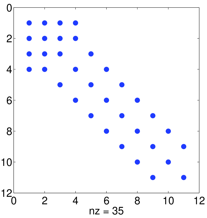
(a) $\left[M\right]$, ST basis.

(b) $\left[K\right]$, ST basis.

(c) $\left[\hat{K}\right]$, ST basis.

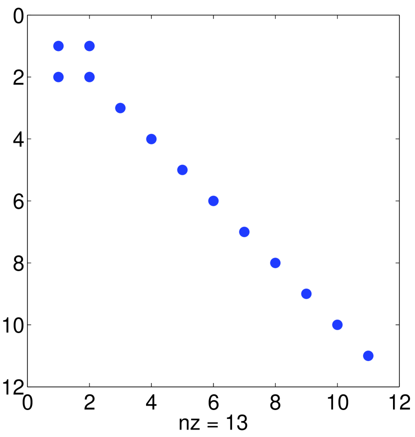
(d) $\left[M\right]$, SDME-M basis.

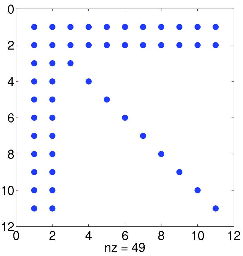
(e) $\left[K\right]$, SDME-M basis.

(f) $\left[\hat{K}\right]$, SDME-H basis.

Figure 2: Sparsity profiles of the mass, stiffness and effective stiffness one-dimensional local matrices for $P=10$ using the standard (ST) and SDME bases with $\lambda=1$.

Figure 3 illustrates the condition numbers for the 1D element local mass and stiffness matrices for orders up to 10 obtained using the SDME-M basis and for the local equivalent stiffness element matrices for the SDME-H basis. It may be observed that parameter $k$ affects the conditioning. The element local mass matrices calculated with the SDME-M basis and $k=\frac{1}{2}$ have condition numbers lower than the respective ones of the ST basis and increasing slightly with the polynomial order. For $k=1$, the stiffness matrices calculated with the SDME-M basis have constant condition numbers and equal to 1 for any polynomial order. Again for $k=1$, the equivalent stiffness matrix with the SDME-H basis has almost constant condition numbers for any order. These features will be similar for multidimensional elements and have positive influence on the number of iterations for the conjugate gradient method which will increase slightly for higher polynomial orders as shown in Section 5. Aspects related to the sparsity of element matrices and the influence of parameter $\lambda$ in the conditioning of matrices calculated with the SDME-H basis are presented in [27].

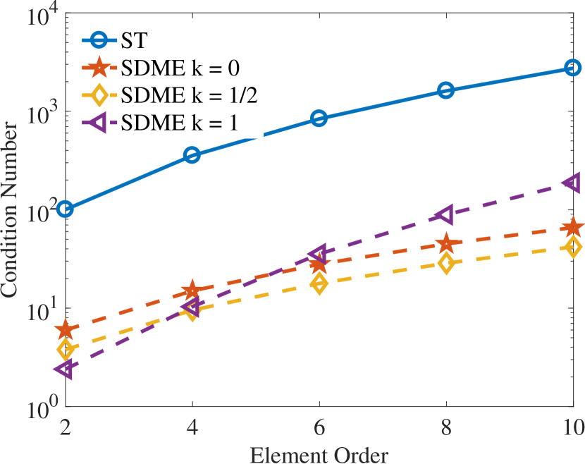
(a) $\left[M\right]$, ST and SDME-M bases.

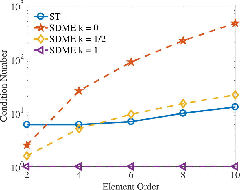
(b) $\left[K\right]$, ST and SDME-M bases.

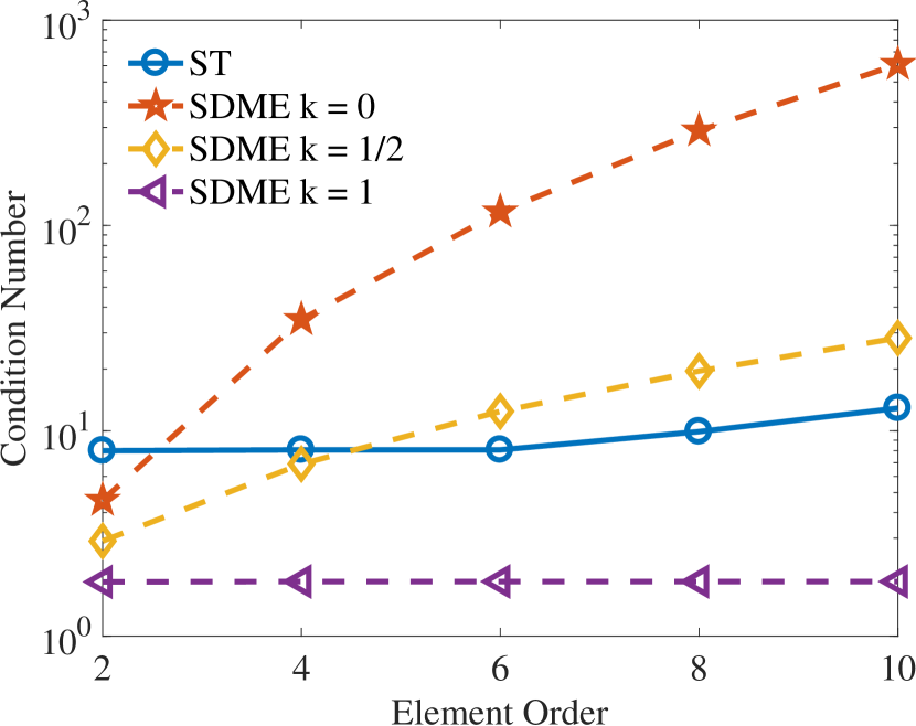
(c) $\left[\hat{K}\right]$, ST and SDME-H bases.

Figure 3: Condition numbers for the mass, stiffness and equivalent element matrices using the standard (ST), SDME-M and SDME-H bases with $\lambda=1$.

The shape functions for squares and hexahedra are obtained using the tensor product of the previously developed one-dimensional functions, respectively, in the local coordinate systems $\xi_{1}\times\xi_{2}$ and $\xi_{1}\times\xi_{2}\times\xi_{3}$ [1, 8, 2]:

$$N_{i}(\xi_{1},\xi_{2}) = \varphi_{p}(\xi_{1})\varphi_{q}(\xi_{2})\;\;(0\leq p,q\leq P),$$ (23)

$$N_{i}(\xi_{1},\xi_{2},\xi_{3}) = \varphi_{p}(\xi_{1})\varphi_{q}(\xi_{2})\varphi_{r}(\xi_{3})\;\;(0\leq p,q,r\leq P),$$ (24)

where $p$, $q$ and $r$ represent the tensor product indices associated with the topological entities of the element; $P$ denotes the polynomial order in directions $\xi_{1}$, $\xi_{2}$ and $\xi_{3}$; $i=1,\ldots,(P+1)^{2}$ for squares and $i=1,\ldots,(P+1)^{3}$ for hexahedra. The SDME bases are hierarchical, conforming and continuous on the element boundaries.

It is possible to define procedures to construct the tensor indices $p$, $q$ and $r$ for any polynomial order $P$. Observe that as the polynomial order increases, the number of body shape functions of hexahedron increases very fast with the cubic power of $P$. In this way, it is very important to construct the shape functions using the tensor product of the one-dimensional functions, avoiding large memory demand.

The shape functions of squares are associated with the element topological entities, which include four vertices $(V_{1},V_{2},V_{3},V_{4})$, four edges $(E_{1},E_{2},E_{3},E_{4})$, and one face $(F_{1})$, illustrated in Figure 4(b). The indices $p$ and $q$ of Equation (23) are associated to the topological entities according to Figure 4(c). The linear, quadratic and cubic square standard elements are illustrated in Figure 5 in the local coordinate system $\xi_{1}\times\xi_{2}$. Vertex and edge nodes/modes defines the boundary modes while the face ones define the internal set. Schur complement of the element matrices are calculated to condense the contribution of the internal to the boundary DOFs.

(a) Indices $p$ and $q$.

(b) Topological entities.

(c) Entities and indices $p$ and $q$.

Figure 4: Association between the topological entities and tensor indices $p$ and $q$ in the square [8].

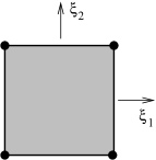
(a) Linear.

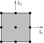
(b) Quadratic

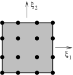
(c) Cubic.

Figure 5: Linear, quadratic and cubic squares [8].

3 Weak form of the boundary value problem

Given a deformation state $\varphi_{k}$ of a three-dimensional body and an arbitrary virtual displacement $\delta\mathbf{u}$ kinematically admissible in the current position, we can write the total Lagrangian description of the principle of virtual work for elastodynamics as: find the displacement vector field $\mathbf{u}\in V_{t}$ such that for $\forall\delta\mathbf{u}\in V$ [48]

$$\delta\Pi_{s}\left(\varphi_{k},\mathbf{u}\right)=\int_{\Omega_{0}}\rho_{0}\frac{\partial^{2}\mathbf{u}}{\partial t^{2}}\cdot\delta\mathbf{u}d\Omega+\int_{\Omega_{0}}\mathbf{S}\colon\delta\mathbf{E}d\Omega-\int_{\Omega_{0}}\rho_{0}\mathbf{f}\cdot\delta\mathbf{u}d\Omega-\int_{\Gamma_{\sigma}}\bar{\mathbf{t}}\cdot\delta\mathbf{u}d\Gamma_{\sigma},$$ (25)

where $\Omega$ denotes the current domain occupied by the body with boundary $\partial\Omega=\Gamma_{\sigma}\bigcup\Gamma_{u}$ and $\Gamma_{\sigma}\bigcap\Gamma_{u}=\emptyset$. $\Gamma_{\sigma}$ and $\Gamma_{u}$ denote the Neumann and Dirichlet boundaries with prescribed tractions ($\bar{\mathbf{t}}$) and displacement ($\bar{\mathbf{u}}$) vector fields, respectively. The term $\mathbf{S}$ is the second Piolla-Kirchhoff tensor, $\delta\mathbf{u}$ is the virtual displacement vector field from the current position, $\delta\mathbf{E}$ is the associated virtual Green strain tensor, $\rho_{0}$ is the mass density, $\mathbf{f}$ is the vector field of body forces. $V_{t}$ is the standard solution space for elastodynamics and $V$ the test space, respectively, defined as

$$V_{t} = \left\{\mathbf{u}\in H^{\text{1}}\left(\varOmega\right)\colon\mathbf{u}=\bar{\mathbf{u}}\left(\mathbf{x},t\right)\mbox{ for }\mathbf{x}\mbox{ on }\Gamma_{u}\right\},$$ (26)

$$V = \left\{\mathbf{w}\in H^{\text{1}}\left(\varOmega\right)\colon\mathbf{w}\left(\mathbf{x}\right)=0\mbox{ for }\mathbf{x}\mbox{ on }\Gamma_{u}\right\}.$$ (27)

$H^{1}\left(\Omega\right)$ is the Hilbert space of all vector valued functions over $\Omega$ which together with their first derivatives are square integrable over the domain.

We use the neo-Hookean hyperelastic material for describing the nonlinear elastic constitutive model. The corresponding strain energy density function is defined as

$$\Psi=\frac{\mu}{2}\left[\mbox{tr}\left(\mathbf{C}\right)-3\right]-\mu\text{ln}J+\frac{\lambda}{2}\left(\text{ln}J\right)^{2},$$ (28)

where $\mathbf{C}$ is the right Cauchy-Green deformation tensor directly related to $\mathbf{E}=\frac{1}{2}\left(\mathbf{C}-\mathbf{I}\right)$, $J=\det\mathbf{F}$, where $\mathbf{F}$ is the gradient of deformation tensor and $\ln\left(J\right)$. The terms $\mu$ and $\lambda$ are the Lamè parameters [49]. The constitutive equation for the second Piola-Kirchhoff stress is

$$\mathbf{S}=\frac{\partial\Psi}{\partial\mathbf{E}}=2\frac{\partial\Psi}{\partial\mathbf{C}}=\mu\left(\mathbf{I}-\mathbf{C}^{-1}\right)+\lambda\left(\text{ln}J\right)\mathbf{C}^{-1}.$$ (29)

The first term in (25) is the virtual work of the inertia denoted by $\delta\Pi^{ine}\left(\varphi_{k},\delta\mathbf{u}\right)$. We use $\delta\Pi^{int}\left(\varphi_{k},\delta\mathbf{u}\right)$ to denote the second term in (25), which represents the internal virtual work due to the stresses and is nonlinear with respect to the displacement field. The third and fourth terms represent the virtual work of the external loads and denoted by $\delta\Pi^{ext}\left(\varphi_{k},\delta\mathbf{u}\right)$. Therefore, Eq.(25) can be rewritten as

$$\delta\Pi_{s}\left(\varphi_{k},\delta\mathbf{u}\right) = \delta\Pi^{ine}\left(\varphi_{k},\delta\mathbf{u}\right)+\delta\Pi^{int}\left(\varphi_{k},\delta\mathbf{u}\right)-\delta\Pi^{ext}\left(\varphi_{k},\delta\mathbf{u}\right)=\delta\hat{\mathbf{u}}^{T}\psi,$$ (30)

where $\psi$ is the residue vector.

Equation (30) can be linearized in the direction of a displacement increment $\Delta\mathbf{u}$, using a first order Taylor expansion about the trial point

$$\delta\Pi_{s}\left(\varphi_{k},\delta\mathbf{u}\right)+D\delta\Pi_{s}\left(\varphi_{k},\delta\mathbf{u}\right)\Delta\mathbf{u}=0.$$ (31)

In the HOFEM, the element displacement field, virtual displacement field and material coordinates can be interpolated in each element similarly to the standard FEM, respectively as

$$\mathbf{u}^{e}(\boldsymbol{\xi})=\sum_{i=1}^{N_{me}}N_{i}(\boldsymbol{\xi})\hat{\mathbf{u}}_{i},$$ (32)

$$\delta\mathbf{u}^{e}(\boldsymbol{\xi})=\sum_{i=1}^{N_{me}}N_{i}(\boldsymbol{\xi})\delta\hat{\mathbf{u}}_{i},$$ (33)

$$\mathbf{X}^{e}(\boldsymbol{\xi})=\sum_{i=1}^{N_{me}}N_{i}(\boldsymbol{\xi})\hat{\mathbf{X}}_{i},$$ (34)

where $N_{me}$ is the number of modes per element, $N_{i}$ are the shape functions and $\boldsymbol{\xi}$ is the local coordinate system (for square $\boldsymbol{\xi}=\xi_{1}\times\xi_{2}$) and hexahedra $\boldsymbol{\xi}=\xi_{1}\times\xi_{2}\times\xi_{3}$. $\hat{\mathbf{u}}_{i}$, $\delta\hat{\mathbf{u}}_{i}$ and $\hat{\mathbf{X}}_{i}$ are the expansion coefficients for the displacement field, virtual displacement field and material coordinates, respectively.

The first term in (31) is the virtual work and the derivative in the second term gives rise to the effective tangent stiffness matrix $\hat{\mathbf{K}}\left(\varphi_{k},\delta\mathbf{u}\right)$ using the previous approximations. Therefore,

$$D\delta\Pi_{s}\left(\varphi_{k},\delta\mathbf{u}\right)\Delta\mathbf{u} = D\left[\delta\Pi^{ine}+\delta\Pi^{int}-\delta\Pi^{ext}\right]\Delta\mathbf{u}=\delta\hat{\mathbf{u}}^{T}\hat{\mathbf{K}}\Delta\mathbf{u}.$$ (35)

Finally, we can rewrite (31) as

$$\delta\hat{\mathbf{u}}^{T}\left(\psi+\delta\hat{\mathbf{u}}^{T}\hat{\mathbf{K}}\Delta\right)=0.$$ (36)

Once the virtual displacements are arbitrary, we can solve (36) iteratively to find $\Delta\mathbf{u}$. Detailed description on the derivation of the weak form of the BVP, including the directional derivatives $D\delta\Pi^{ine}\Delta\mathbf{u}$ and $D\delta\Pi^{int}\Delta\mathbf{u}$, can be found in [49].

4 Non-linear elastodynamics

In this section we present the equation for conservation of linear momentum in discrete form, and show the explicit central difference and implicit Newmark time-integration schemes employed, with the respective expressions after applying the Schur complement to condense the internal modes.

4.1 Explicit time integration

We consider the equation of motion (30) in discrete form for the current time $t_{n}$, neglecting damping effects, for non-linear elastic problems, which is given by

$$\mathbf{M}\mathbf{a}_{n}+\mathbf{R}\left(\mathbf{u}_{n}\right)=\mathbf{P}_{n},$$ (37)

with $\mathbf{M}$ denoting the global mass matrix in the reference configuration, $\mathbf{a}_{n}=\ddot{\boldsymbol{u}}_{n}$ the global acceleration vector, $\mathbf{R}\left(\mathbf{u}_{n}\right)$ the global internal force vector and $\mathbf{P}_{n}$ the global external load vector. The velocities $\mathbf{v}_{n}$ and accelerations $\mathbf{a}_{n}$ can be approximated using the central-difference schemes in the following ways:

$$\mathbf{v}_{n}=\frac{\mathbf{u}_{n+1}-\mathbf{u}_{n-1}}{2\Delta t},\quad\quad\mathbf{a}_{n}=\frac{\mathbf{u}_{n+1}-2\mathbf{u}_{n}+\mathbf{u}_{n-1}}{{\Delta t}^{2}}.$$ (38)

Substituting the accelerations $\mathbf{a}_{n}$ from Eq.(38) into Eq.(37) and rearranging the terms, we obtain

$$\hat{\mathbf{M}}\mathbf{u}_{n+1}=\boldsymbol{\psi}_{n}+\hat{\mathbf{M}}\left(2\mathbf{u}_{n}-\mathbf{u}_{n-1}\right),$$ (39)

with,

$$\hat{\mathbf{M}}=\frac{1}{{\Delta t}^{2}}\mathbf{M},$$ (40)

$$\boldsymbol{\psi}_{n}=\mathbf{P}_{n}-\mathbf{R}\left(\mathbf{u}_{n}\right).$$ (41)

Therefore, we must solve Eq.(39) to determine the displacements at time $t_{n+1}$. Considering initial conditions for the displacements and velocities ($\mathbf{u}_{0}$, $\mathbf{v}_{0}$ known), the initial condition for the acceleration can be obtained by setting $t=t_{0}$ in Eq.(37). Therefore,

$$\mathbf{a}_{0}=\mathbf{M}^{-1}\boldsymbol{\psi}_{0}.$$ (42)

The displacement for time $t=t_{-1}$ can be obtained with Eq.(38) and is given by

$$\mathbf{u}_{-1}=\mathbf{u}_{0}-\Delta t\mathbf{v}_{0}+\frac{{\Delta t}^{2}}{2}\mathbf{a}_{0}.$$ (43)

We can express Eq.(39) in terms of the boundary and internal modes in the following form:

$$\begin{bmatrix}\hat{\mathbf{M}}_{bb}&\hat{\mathbf{M}}_{bi}\\ \hat{\mathbf{M}}^{T}_{bi}&\hat{\mathbf{M}}_{ii}\\ \end{bmatrix}\begin{bmatrix}\mathbf{u}_{b}\\ \mathbf{u}_{i}\end{bmatrix}_{n+1}=\begin{bmatrix}\boldsymbol{\psi}_{b}\\ \boldsymbol{\psi}_{i}\end{bmatrix}_{n}+\begin{bmatrix}\hat{\mathbf{M}}_{bb}&\hat{\mathbf{M}}_{bi}\\ \hat{\mathbf{M}}^{T}_{bi}&\hat{\mathbf{M}}_{ii}\\ \end{bmatrix}\begin{bmatrix}\mathbf{u}^{*}_{b}\\ \mathbf{u}^{*}_{i}\end{bmatrix},$$ (44)

with

$$\begin{bmatrix}\mathbf{u}^{*}_{b}\\ \mathbf{u}^{*}_{i}\end{bmatrix}=\begin{bmatrix}2\mathbf{u}_{b}\\ 2\mathbf{u}_{i}\end{bmatrix}_{n}-\begin{bmatrix}\mathbf{u}_{b}\\ \mathbf{u}_{i}\end{bmatrix}_{n-1}.$$ (45)

Expanding Eq.(44) in terms of the boundary modes and dropping the subscripts for time, we obtain the following equations:

$$\hat{\mathbf{M}}_{bb}\mathbf{u}_{b}+\hat{\mathbf{M}}_{bi}\mathbf{u}_{i}=\boldsymbol{\psi}_{b}+\hat{\mathbf{M}}_{bb}\mathbf{u}^{*}_{b}+\hat{\mathbf{M}}_{bi}\mathbf{u}^{*}_{i},$$ (46)

$$\hat{\mathbf{M}}^{T}_{bi}\mathbf{u}_{b}+\hat{\mathbf{M}}_{ii}\mathbf{u}_{i}=\boldsymbol{\psi}_{i}+\hat{\mathbf{M}}^{T}_{bi}\mathbf{u}^{*}_{b}+\hat{\mathbf{M}}_{ii}\mathbf{u}^{*}_{i}.$$ (47)

Multiplying Eq.(47) by $\hat{\mathbf{M}}^{-1}_{ii}$ and solving for $\mathbf{u}_{i}$, we obtain

$$\mathbf{u}_{i}=\mathbf{u}^{*}_{i}+\hat{\mathbf{M}}^{-1}_{ii}\left(\boldsymbol{\psi}_{i}-\hat{\mathbf{M}}^{T}_{bi}\mathbf{u}_{b}+\hat{\mathbf{M}}^{T}_{bi}\mathbf{u}^{*}_{b}\right).$$ (48)

Substituting the above equation into Eq.(46) and rearranging the terms, we have

$$\hat{\mathbf{M}}^{sc}_{b}\mathbf{u}_{b}=\boldsymbol{\psi}^{sc}_{b}+\hat{\mathbf{M}}^{sc}_{b}\mathbf{u}^{*}_{b},$$ (49)

where

$$\hat{\mathbf{M}}^{sc}_{b}=\hat{\mathbf{M}}_{bb}-\hat{\mathbf{M}}_{bi}\hat{\mathbf{M}}^{-1}_{i}\hat{\mathbf{M}}^{T}_{bi},$$ (50)

$$\boldsymbol{\psi}^{sc}_{b}=\boldsymbol{\psi}_{b}-\hat{\mathbf{M}}_{bi}\hat{\mathbf{M}}^{-1}_{i}\boldsymbol{\psi}_{i}.$$ (51)

Finally, we can solve Eq.(49) to obtain

$$\mathbf{u}_{b}=\hat{\mathbf{M}}^{{sc}^{-1}}_{b}\boldsymbol{\psi}^{sc}_{b}+\mathbf{u}^{*}_{b}.$$ (52)

Therefore, we perform the Schur complement on $\hat{\mathbf{M}}_{b}$ and $\boldsymbol{\psi}_{b}$, calculate the coefficients of the boundary modes from Eq.(52) and then recover the coefficients of the internal modes using Eq.(48).

4.2 Implicit time integration (Newmark)

We consider the equilibrium equation (37) for the current time step $t_{n+1}$

$$\mathbf{M}\mathbf{a}_{n+1}+\mathbf{R}_{n+1}=\mathbf{P}_{n+1},$$ (53)

where $\mathbf{M}$ is the global mass matrix, $\mathbf{R}_{n+1}$ the global internal force vector dependent on the updated configuration with coordinates $\mathbf{x}_{n+1}$, which in turn depend on the displacements $\mathbf{u}_{n+1}$. The term $\mathbf{P}_{n+1}$ represents the global external nodal force vector. The terms $\mathbf{a}_{n+1}$ and $\mathbf{v}_{n+1}$ respectively denote the global acceleration and velocity vectors at time step $t_{n+1}$.

We define the following residue force vector $\boldsymbol{\psi}_{n+1}$ at time step $t_{n+1}$:

$$\boldsymbol{\psi}_{n+1}=\mathbf{M}\mathbf{a}_{n+1}+\mathbf{R}_{n+1}-\mathbf{P}_{n+1}=\mathbf{0}.$$ (54)

The following approximations for the velocity and accelerations are used by the Newmark method [50]:

$$\mathbf{a}_{n+1} =b_{1}\left(\mathbf{u}_{n+1}-\mathbf{u}_{n}\right)-b_{2}\mathbf{v}_{n}-b_{3}\mathbf{a}_{n},$$ (55)

$$\mathbf{v}_{n+1} =b_{4}\left(\mathbf{u}_{n+1}-\mathbf{u}_{n}\right)-b_{5}\mathbf{v}_{n}-b_{6}\mathbf{a}_{n},$$ (56)

with the coefficients

$$\begin{array}[]{ccc}b_{1}=\frac{1}{g_{1}\Delta t^{2}},&b_{2}=\frac{1}{g_{1}\Delta t},&b_{3}=\frac{1-2g_{1}}{2g_{1}},\\ b_{4}=\frac{g_{2}}{g_{1}\Delta t^{2}},&b_{5}=\left(1-\frac{g_{2}}{g_{1}}\right),&b_{6}=\left(1-\frac{g_{2}}{2g_{1}}\right)\Delta t.\end{array}$$

Here, we choose $g_{1}=0.5$ to obtain quadratic convergence in time and $g_{2}=0.25$ for unconditional stability. Substituting Eq.(55) in Eq.(54), we obtain

$$\boldsymbol{\psi}_{n+1}=\mathbf{M}\left[b_{1}\left(\mathbf{u}_{n+1}-\mathbf{u}_{n}\right)-b_{2}\mathbf{v}_{n}-b_{3}\mathbf{a}_{n}\right]+\mathbf{R}_{n+1}-\mathbf{P}_{n+1}=\mathbf{0},$$ (57)

The equilibrium system, Eq.(57), is linearized with the Newton-Raphson method using incremental global displacements defined as

$$\mathbf{u}^{k+1}_{n+1}=\mathbf{u}^{k}_{n+1}+\Delta\mathbf{u}.$$ (58)

Accordingly, the updated global coordinates are given by

$$\mathbf{x}^{k+1}_{n+1}=\mathbf{x}_{n}+\mathbf{u}^{k+1}_{n+1},$$ (59)

where the superscript $k+1$ refers to the current iteration of the Newton method.

The linearized form of Eq.(57) in the direction of a displacement increment $\Delta\mathbf{u}$ is given by the following system of equations:

$$\left[b_{1}\mathbf{M}+\mathbf{K}^{k}_{T_{n+1}}\right]\Delta\mathbf{u}=-\mathbf{M}\left[b_{1}(\mathbf{u}^{k}_{n+1}-\mathbf{u}_{n})-b_{2}\mathbf{v}_{n}-b_{3}\mathbf{a}_{n}\right]-\mathbf{R}^{k}_{n+1}+\mathbf{P}_{n+1},$$ (60)

where the terms $\mathbf{u}_{n}$, $\mathbf{v}_{n}$, $\mathbf{a}_{n}$ are known from the last converged time step $t_{n}$. The term $\mathbf{K}_{T}$ is the tangent stiffness matrix and is updated at each iteration $k$ along with the internal force vector.

Now we consider the application of the Schur complement for the system given by Eq.(60). We will drop the scripts $n+1$ and $k$ for simplicity. Consider Eq.(60) rewritten in the following form:

$$\hat{\mathbf{K}}\boldsymbol{\Delta u}=\boldsymbol{\psi},$$ (61)

where $\hat{\mathbf{K}}$ denotes the effective tangent stiffness matrix, given by

$$\hat{\mathbf{K}}=b_{1}\mathbf{M}+\mathbf{K}^{T},$$ (62)

and $\boldsymbol{\psi}$ represents the residual force vector

$$\boldsymbol{\psi}=-\mathbf{M}\mathbf{a}-\mathbf{R}^{k}_{n+1}+\mathbf{P}_{n+1}.$$ (63)

Differently from the explicit method, we apply the Schur complement directly on the equivalent system, Eq.(61), since we work with an equivalent global matrix in this case. The previous equation can be written in terms of boundary, internal and coupled matrix blocks as

$$\begin{bmatrix}\hat{\mathbf{K}}_{bb}&\hat{\mathbf{K}}_{bi}\\ \hat{\mathbf{K}}^{T}_{bi}&\hat{\mathbf{K}}_{ii}\\ \end{bmatrix}\begin{bmatrix}\Delta\mathbf{u}_{b}\\ \Delta\mathbf{u}_{i}\end{bmatrix}=\begin{bmatrix}\boldsymbol{\psi}_{b}\\ \boldsymbol{\psi}_{i}\end{bmatrix},$$ (64)

where, after applying the Schur complement, we have

$$\left(\hat{\mathbf{K}}_{bb}-\hat{\mathbf{K}}_{bi}\hat{\mathbf{K}}^{-1}_{ii}\hat{\mathbf{K}}^{T}_{bi}\right)\Delta\mathbf{u}_{b}=\left(\boldsymbol{\psi}_{b}-\hat{\mathbf{K}}_{bi}\hat{\mathbf{K}}^{-1}_{ii}\boldsymbol{\psi}_{i}\right),$$ (65)

$$\Delta\mathbf{u}_{i}=\hat{\mathbf{K}}^{-1}_{ii}\left(\boldsymbol{\psi}_{i}-\hat{\mathbf{K}}^{T}_{bi}\Delta\mathbf{u}_{b}\right).$$ (66)

We can rewrite the linearized equilibrium system (60) using the nonlinear Newmark time integration scheme to the contact problem as [51, 52]

$$\left[b_{1}\mathbf{M}+\mathbf{K}^{k}_{T_{n+1}}+\mathbf{K}_{T_{n+1}}^{c^{k}}\right]\Delta\mathbf{u} = -\mathbf{M}\left[b_{1}(\mathbf{u}^{k}_{n+1}-\mathbf{u}_{n})-b_{2}\mathbf{v}_{n}-b_{3}\mathbf{a}_{n}\right]$$ (67)

$$-\mathbf{R}^{k}_{n+1}+\mathbf{P}_{n+1}-\mathbf{F}_{n+1}^{c^{k}},$$

where $\mathbf{K}^{c}_{T}$ and $\mathbf{F}^{c}$ are the global contact tangent stiffness matrix and force vector after the application of the high-order finite element approximations.

5 Numerical results

In this section, we analyze the performance of the SDME-M and SDME-H modal bases compared to the standard Jacobi modal (ST) basis in terms of the number of iterations and and computational time for linear system solution, using the conjugate gradient method with the Gauss-Seidel (CGGS) and the diagonal (CGD) pre-conditioners [53]. The first example considers the static analysis of a large strain problem with fabricated solution comparing the convergence behavior of the bases. Section 5.2 presents analyses of transient problems with fabricated solutions using explicit and implicit time integration to verify spatial convergence and second-order time rate. Section 5.2 shows the explicit and implicit analyses of a 3D conrod submitted to a transient dynamic load calculated from the pressure curve of a four stroke engine. The polynomial orders are increased and the results in terms of number of iterations and speedup are presented. Sections 5.4 and 5.5 presents the analyses of 2D and 3D frictionless impact problems, respectively. In Section 5.5, results for the Lagrange nodal basis with Gauss-Lobatto-Legendre collocation points are included. All the examples use a Neohookean hyperelastic material model with Lagragian description.

5.1 Static non-linear problem with large strains

To verify the performance and accuracy of the standard and minimum energy bases, we consider the cube domain with coordinates $0\leq x,y,z\leq 1$ discretized using 8 hexahedra and the fabricated solution with the following displacement components:

$$u_{x}=1.9\sin(x)-x,\quad u_{y}=0,\quad u_{z}=0.$$ (68)

The Young’s modulus and Poisson ratio are respectively $E=1000\,Pa$ and $\nu=0.3$.

We consider the ST, SDME-M and SDME-H ($\lambda=100$) bases with $k=0.5$. We compute the average number of iterations of the conjugate gradient method with diagonal preconditioner (CGD) and time (for linear system solution) per Newton-Raphson iteration. The CGD tolerance is chosen as $10^{-12}$ and the Newton solver tolerance is set to $10^{-8}$. We perform the Schur complement on the tangent stiffness matrix and residual (out-of-balance) force vector. We also considered isoparametric mapping.

The obtained spectral accuracy results are presented in Table 1, which are identical for all employed bases. From Table 2, we observe that the standard basis require $7.85$ times more iterations when compared to the SDME-M basis for $P=8$. The same ratio is obtained for the average time in Table 3. The SDME-H basis provided better performance than the SDME-M basis for $P<8$.

Table 1: $L_{2}$ error norms for the displacement components of the static analysis using the ST, SDME-M and SDME-H bases.

Order	Number of DOFs	$L_{2}$ error
		$u_{x}$	$u_{y}$	$u_{z}$
2	300	1.09e-03	1.83e-04	1.68e-04
4	1944	7.01e-07	1.22e-07	1.34e-07
6	6084	4.51e-09	8.47e-10	7.98e-10
8	13872	8.15e-11	1.21e-11	1.20e-11

Table 2: Average numbers of CGD iterations per Newton iteration, total of 5 Newton iterations for convergence, for the static problem of fabricated solution.

Order	Number of DOFs	Average number of CGD iterations
		ST	SDME-M	SDME-H
2	300	75.8	43.2	41.2
4	1 944	249.4	67.2	57.0
6	6 084	444.4	81.8	64.0
8	13 872	660.0	84.0	95.0

Table 3: Average time for CGD solution per Newton iteration for the static problem of fabricated solution.

Order	Number of DOFs	Average time for CGD solution [s]
		ST	SDME-M	SDME-H
2	300	0.0042	0.0024	0.0023
4	1 944	0.2230	0.0598	0.0501
6	6 084	2.0236	0.3760	0.2464
8	13 872	9.7028	1.2363	1.4031

The same analysis was performed using the conjugate gradient method with the Gauss-Seidel preconditioner (CGGS). The results are presented in Tables 4 and 5, showing a better performance of the SDME-H basis for all polynomial orders.

Table 4: Average number of CGGS iterations per Newton iteration, total of 5 Newton iterations for convergence, for the static problem of fabricated solution.

Order	Number of DOFs	Average number of CGGS iterations
		ST	SDME-M	SDME-H
2	300	61.2	49.6	47.8
4	1 944	132.0	60.4	52.6
6	6 084	218.2	66.4	51.6
8	13 872	313.0	65.4	56.6

Table 5: Average time for CGGS solution per Newton iteration for the static problem of fabricated solution.

Order	Number of DOFs	Average time for CGGS solution [s]
		ST	SDME-M	SDME-H
2	300	0.0031	0.0026	0.0023
4	1 944	0.1037	0.0496	0.0419
6	6 084	0.8952	0.2856	0.2389
8	13 872	4.2829	0.9190	0.7569

5.2 Transient nonlinear problems with large strains

5.2.1 Explicit time integration

In this case, we consider the same mesh of the previous example, time interval $t=[0,\,0.25]\,s$ and the following fabricated solution:

$$u_{x}=\sin\left(\frac{\pi}{2}x\right)\sin(2\pi t),\quad u_{y}=0,\quad u_{z}=0,$$ (69)

which gives $u_{x}=1.0$  m for $x=1.0$ and $t=0.25\,s$. The material properties are $E=1000\,Pa$, $\nu=0.3$ and $\rho=1\,kg/m^{3}$. Homogeneous Dirichlet boundary conditions are applied in all displacement directions of the face with coordinate ${x}=0$.

We used the CFL condition to estimate the number of time steps as [50]:

$$\Delta t\leq\delta\frac{h}{c_{L}},$$ (70)

where $h$ represents the element size (considered as the edge length in the initial configuration for this problem), $\delta$ denotes a constant in the range $0.2<\delta<0.9$ and

$$c_{L}=\frac{3K(1-\nu)}{\rho(1+\nu)},\qquad K=\frac{E}{3(1-2\nu)}.$$ (71)

Considering the given material properties and $\delta=0.85$, we obtained $\Delta t=3.33\times 10^{-4}$ and $N=800$ times steps for the analysis with a single load step.

Initially, we performed spatial convergence analysis by increasing the polynomial approximation orders. Tables 6 and 7 show the $L_{2}$ error norms for the displacement components using the ST and SDME-M bases, respectively. We may observe spectral spatial convergence rates using the two bases. Furthermore, we compare the employed bases with a standard Lagrange basis with a diagonal mass matrix in Table 8. We observe that the Lagrange basis with a diagonal mass matrix yields slightly higher errors for the $x$-direction due to the decreased number of integration points.

Table 6: $L_{2}$ error norms for the displacement components of explicit analysis using the ST basis.

Order	Number of DOFs	$L_{2}$ error
		$u_{x}$	$u_{y}$	$u_{z}$
2	276	2.08e-3	2.45e-4	2.26e-4
4	1246	3.38e-6	5.16e-7	5.61e-7
6	3084	4.21e-8	6.09e-9	5.76e-9

Table 7: $L_{2}$ error norms for the displacement components of explicit analysis using the SDME-M basis.

Order	Number of DOFs	$L_{2}$ error
		$u_{x}$	$u_{y}$	$u_{z}$
2	276	2.09e-3	2.53e-4	2.34e-4
4	1246	3.36e-6	5.06e-7	5.51e-7
6	3084	4.21e-8	6.08e-9	5.76e-9

Table 8: $L_{2}$ error norms for the displacement components of the explicit analysis utilizing a Lagrange basis yielding a diagonal mass matrix.

Order	Number of DOFs	$L_{2}$ error
		$u_{x}$	$u_{y}$	$u_{z}$
2	276	2.12e-03	2.78e-04	2.78e-04
4	1246	3.75e-06	4.44e-07	4.44e-07
6	3084	5.29e-08	5.50e-09	5.50e-09

We compared the performance of the ST and SDME-M bases for the average number of iterations and average time using the conjugate gradient method with the Gauss-Seidel (CGGS) preconditioner to solve the linear system of equations with tolerance of $10^{-12}$. The results for the number of iterations are presented in Table 9 and the computational times per time step are given in Table 10. The SDME-M basis improved the standard Jacobi modal basis about 18 times.

Table 9: Average number of iterations for convergence using the CGGS method for the fabricated solution and explicit time integration.

Order	ST	SDME-M	Ratio ST/SDME
2	68.37	9.99	6.84
4	172.19	7.97	21.60
6	297.48	16.48	18.05

Table 10: Average time per time step using the CGGS methods for the ST and SDME-M bases for the fabricated solution and explicit time integration.

Order	ST [s]	SDME-M [s]	Speedup
2	0.0153	0.0026	5.88
4	0.6279	0.0363	17.30
6	5.7101	0.3537	16.43

5.2.2 Implicit time integration

For the implicit Newmark integration method, we first consider the following fabricated solution for $u(x,t)$:

$$u_{x}=x^{4}\sin(2\pi t),\quad u_{y}=0,\quad u_{z}=0.$$ (72)

The total time is $T=0.025\,s$ and the solution gives $u_{x}=0.157\,m$ for $x=1.0\,m$ and $t=0.025\,s$. The material properties and boundary conditions are the same of the previous example. The tolerance for the residue norm in the Newton method is $10^{-12}$. We tested the performance of bases ST, SDME-M, SDME-H with $k=0.5$ and $\lambda=100$ in terms of the average number of iterations, average times and speedup. using the CGGS method. The results are presented in Figs. 6 and 7. We observe that the SDME-M basis performed better than the SDME-H basis, with a speedup up to 19 with polynomial order $P=4$. The SDME-H basis achieved at least a speedup ratio of 3 compared to the ST basis as illustrated in Fig. 7.

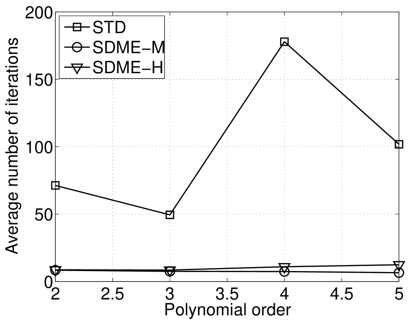
(a) Average number of iterations.

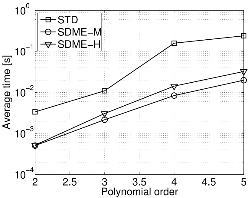
(b) Average time.

Figure 6: Average number of iterations for linear system solution using CGGS method in terms of the polynomial order, $\Delta t=3.90\times 10^{-4}\,s$ (a); Average time for linear system solution in terms of the polynomial order (b).

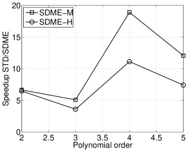
Figure 7: Speedup ratio for the computation time to solve the linear system of equations between the standard Jacobi basis and the minimum energy bases SDME-M and SDME-H with $k=0.5$ and $\lambda=100$.

We also considered the solution using the CGD method. The results are presented in Figs. 8 and 9. Similarly to the CGGS preconditioner, both minimum energy bases performed much better than the ST basis, with speedups up to 26 for the SDME-M basis. In general, the speedup achieved by the SDME-M basis was also larger than the SDME-H basis.

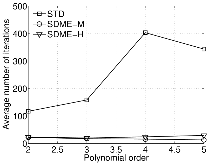
(a) Average number of iterations.

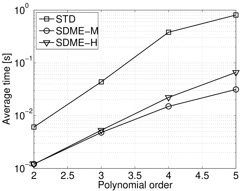
(b) Average time.

Figure 8: Average number of iterations for linear system solution using the CGD method in terms of the polynomial order, $\Delta t=3.90\times 10^{-4}\,s$ (a); Average time for linear system solution in terms of the polynomial order (b).

Figure 9: Speedup ratio for the computation time to solve the linear system of equations between the standard Jacobi basis and the minimum energy bases SDME-M and SDME-H with $k=0.5\,\lambda=100$.

The solution given in Eq.(69) was also considered and the results are presented in Tables 11, 12 and 13. The $L_{2}$ error norms for the displacement components in Table 11 are with the same order of magnitude to those ones of Tables 6 and 7 . We observe that the performance of the SDME-H basis is slightly better than the SDME-M for $P=2,4$ and the SDME-M basis is better for $P=6$.

Table 11: $L_{2}$ error norm using the Newmark method and SDME-H basis for 8 hexahedra, $\Delta t=2\times 10^{-3}\,s$.

Order	Number of DOFs	$L_{2}$ error
		$u_{x}$	$u_{y}$	$u_{z}$
2	276	2.09e-3	2.54e-4	2.35e-4
4	1246	3.40e-6	5.09e-7	5.54e-7
6	3084	9.17e-8	2.23e-8	2.22e-8

Table 12: Average number of iterations for convergence using the CGD method for the ST, SDME-M ($k=0.5$), and SDME-H ($k=0.5,\,\lambda=100$) bases and Newmark integration, $\Delta t=2\times 10^{-3}\,s$.

Order	ST	SDME-M	SDME-H	Ratio ST/SDME-M	Ratio ST/SDME-H
2	119.65	21.40	20.86	5.59	5.74
4	352.05	19.45	17.94	18.10	19.62
6	610.83	32.28	42.01	18.92	14.54

Table 13: Average time per linear system solution using the CGD method for the ST, SDME-M ($k=0.5$), and SDME-H ($k=0.5,\,\lambda=100$) bases and Newmark integration, $\Delta t=2\times 10^{-3}\,s$.

Order	ST (s)	SDME-M (s)	SDME-H (s)	Speedup	Speedup
2	0.0066	0.0011	0.0012	6.000	5.500
4	0.3167	0.0185	0.0176	17.119	17.994
6	2.8062	0.1561	0.1963	17.977	14.295

We now consider spatial convergence using fixed $\Delta t=3.90\times 10^{-4}\,s$ and polynomial orders 2 to 6 and results for both cases are shown in Figure 10 for the $L_{2}$ and $L_{\infty}$ norms. The $L_{2}$ error norm dropped about 1000 times when increasing the polynomial order from 2 to 3 and from 3 to 4, indicating exponential spatial convergence. The time convergence is analysed with fixed $P=5$ and decreasing the time increments $\Delta t$. The time rate was quadratic as expected for the Newmark method.

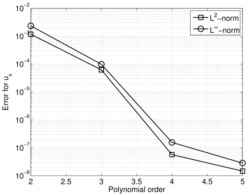
(a) Spatial convergence.

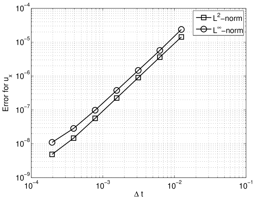
(b) Time convergence.

Figure 10: Spatial convergence for $\Delta t=3.90\times 10^{-4}\,s$ and polynomial orders $P=2,3,4,5$ (a); Convergence in time with $P=5$ and decreasing the time increment $\Delta t$ (b).

5.3 Conrod

We consider now the transient dynamic analysis of the conrod illustrated in Fig. 11 and discretized using 768 hexahedra. Homogeneous Dirichlet boundary conditions ($u_{x}=u_{y}=u_{z}=0$) are applied on the nodes of the internal surface of the small end. The conrod is subjected to a time dependent distributed load on the internal element faces of the big end in directions $x$ and $y$. The material model is the compressible Neo-Hookean with $E=500\,Pa$, $\nu=0.3$, $\rho=9.5\times 10^{-7}\,Kg/m^{3}$. For the SDME bases, we used $\lambda=100$ and $k=0.5$.

The total simulation time is $T=5.454\times 10^{-3}\,s$ which corresponds to one engine cycle for the rotational speed of $2200\ RPM$. In the explicit analysis, we used the time step $\Delta t=6.06\times 10^{-6}$ for polynomial orders $P=2,\,3$; $\Delta t=3.03\times 10^{-6}$ for $P=4$; $\Delta t=1.51\times 10^{-6}$ for $P=5,\,6,\,7$; and $\Delta t=7.58\times 10^{-7}$ for $P=8$. For the implicit analysis, we considered $\Delta t=1.515\times 10^{-5}$ for all polynomial orders. We solved the linear system of equations using a parallel, element-by-element diagonal preconditioned conjugate gradient method (PCG), with tolerances of $10^{-8}$ and $10^{-4}$ respectively for the explicit and implicit analyses. We also considered the tolerance $10^{-4}$ for the convergence of the Newton sub-iterations in the implicit case. The initial conditions are $\mathbf{u}_{0}=\mathbf{0}\,m$ and $\mathbf{v}_{0}=\mathbf{0}\,m/s$.

Figure 11: Mesh for the conrod discretized with 768 hexahedra and $P=1$. The material properties used for the compressible Neo-Hookean are $E=500\,Pa$, $\nu=0.3$, $\rho=9.5\times 10^{-7}\,Kg/m^{3}$.

Table 14 presents the average number of PCG iterations per time step for the explicit time integration. We observe that the best results are achieved using the SDME-M basis, which is expected, since in the explicit time integration the operator in the left-hand-side is the mass matrix (see Eq.(49)). However, we remark that such behavior can be recovered by the SDME-H basis when we set higher values for $\lambda$ [34]. The results for the speedup ratios are presented in Table 15. Similarly to the number of iterations, we obtained the largest speedups (up to $41.71$) for the SDME-M basis when compared to the ST basis.

Table 14: Average number of iterations per time step for the conrod with explicit time integration using the ST and SDME bases. We observe that the SDME-M basis has the best performance, with a ratio (ST/SDME-M) up to $142.3$. The SDME-H basis increases the number of iterations with the polynomial order with the choice of $\lambda=100$.

Order	Number	Average number of iterations per time step
	of DOFs	ST	SDME-M	SDME-H
2	24 651	283.60	22.90	30.80
3	75 984	205.90	15.70	17.20
4	171 753	688.85	13.70	20.80
5	325 782	403.57	11.88	26.48
6	551 895	1 145.08	12.22	40.65
7	863 916	759.30	11.57	54.23
8	1 275 669	1 706.09	11.99	72.55

Table 15: Computational speedup per time step for the conrod with explicit time integration. We observe that the highest speedup obtained is $41.71$ for the SDME-M basis using polynomial order $P=6$.

Order	Number	Speedup $\bar{t}_{ST}/\bar{t}_{SDME}$
	of DOFs	SDME-M	SDME-H
2	24 651	6.48	2.43
3	75 984	16.40	14.97
4	171 753	25.59	17.02
5	325 782	27.13	16.42
6	551 895	41.71	16.28
7	863 916	35.43	14.90
8	1 275 669	34.34	16.28

Table 16 presents the average number of PCG iterations per time step for the implicit time integration. We observe that the SDME-H basis obtained a smaller number of iterations for $P\leq 4$. However, for higher polynomial orders tested, the SDME-M basis provided the best results, with ratio up to $39.20$ when compared to the ST basis. All bases had a smaller number of iterations compared to the explicit case. However, we observe that although we use higher values of $\Delta t$ for the implicit time integration, we need to perform Newton sub-iterations and recalculate the tangent stiffness matrix at every iteration, which is still more time-consuming than the explicit case.

Table 16: Average number of iterations per time step for the conrod with implicit time integration using the ST and SDME bases. We observe that the SDME-M basis has the best performance.

Order	Number	Average number of iterations per time step
	of DOFs	ST	SDME-M	SDME-H
2	24 651	122.75	10.17	9.75
3	75 984	90.25	7.25	6.92
4	171 753	269.33	8.33	7.42
5	325 782	211.75	8.83	9.00
6	551 895	401.17	10.67	13.08
7	863 916	383.00	12.08	16.50
8	1 275 669	539.08	13.75	21.08

Increasing the polynomial orders from 2 to 8, the numbers of DOFs increased over 51 times while the numbers of iterations of the PCG methods for convergence had a slight increase mainly for the SDME-M basis as can be seen in Tables 14 and 16. This aspect means that the conditions numbers of the global matrices had also slight increase as illustrated for the 1D matrices in Figure 3.

The solution for the displacements over time is shown in Fig.12. We observe that most of the deformation occurs at the bigger end where the loads are applied.

$\begin{array}[]{ccc}\includegraphics[width=130.08731pt]{./Figures/frames-01.eps}&\includegraphics[width=130.08731pt]{./Figures/frames-18.eps}&\includegraphics[width=130.08731pt]{./Figures/frames-36.eps}\\ \includegraphics[width=130.08731pt]{./Figures/frames-54.eps}&\includegraphics[width=130.08731pt]{./Figures/frames-72.eps}&\includegraphics[width=130.08731pt]{./Figures/frames-90.eps}\\ \includegraphics[width=130.08731pt]{./Figures/frames-108.eps}&\includegraphics[width=130.08731pt]{./Figures/frames-124.eps}&\includegraphics[width=130.08731pt]{./Figures/frames-144.eps}\\ \end{array}$

Figure 12: Solution for the displacements and deformed geometry of the conrod over time for the transient analysis obtained with the SDME-M basis.

5.4 Two-dimensional disk impact problem

The next example is the small deformation frictionless impact of a linear elastic disk on a foundation as shown in Fig. 13 [54].

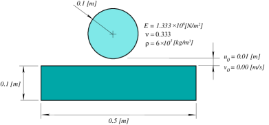
Figure 13: Disk impact problem representation with domain dimensions, material properties and initial conditions.

The implicit Newmark time integration scheme was used. The convergence tolerances used for the CGGS and Newton-Raphson procedures were both $10^{-6}$. The Schur complement was taken for the tangent stiffness matrix and residue vector. The mesh used is illustrated in Fig. 14 and the penalty parameter is $\epsilon_{N}=1.0\times 10^{6}$ and $\Delta\epsilon_{N}=0.0$. The geometry and material properties are presented in Fig 13. We used $P+1$ Gauss-Legendre integration points for the contact elements that were enough to achieve good results. The tolerances for the gap function and contact stress were $10^{-3}$ and $10^{-2}$, respectively .The integration time is $T=0.1\,s$ and $\Delta t=10^{-4}\,s$. The initial conditions are $\mathbf{u}_{0}=\{0.00\;0.01\;0.00\}^{T}\,m$ and $\mathbf{v}_{0}=\mathbf{0}\,m/s$. The foundation was discretized with one finite element with fully constrained edges.

Figure 15 shows the displacement field $u_{y}$ in the deformed geometry for different time steps of the solution for interpolation order $P=1$. Figure 16 shows the comparison of the contact stress field $t_{N}$ for $P=1$ and $P=2$. There is more oscillation in the contact stress field with $P=1$. The oscillation is reduced by increasing the interpolation order, as can be seen in Fig. 16. The increase of the interpolation order induces a better distribution of the mass inside the finite element, reducing the effect caused by the kinetic energy loss in the contact area (velocity became instantly zero at the contact surface).

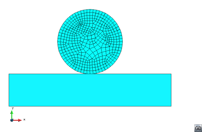
Figure 14: Mesh for the disc impact problem. The disk was meshed with quadrangular elements. The foundation is meshed by one rectangular element and its edges are fully constrained

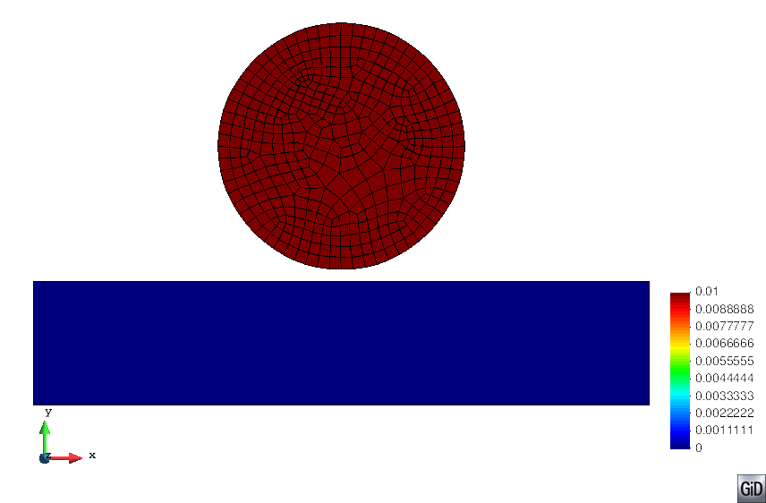
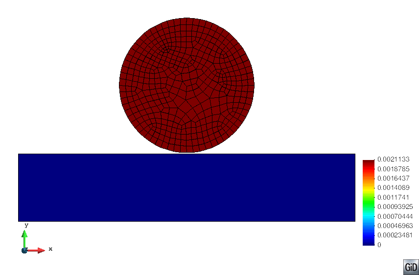
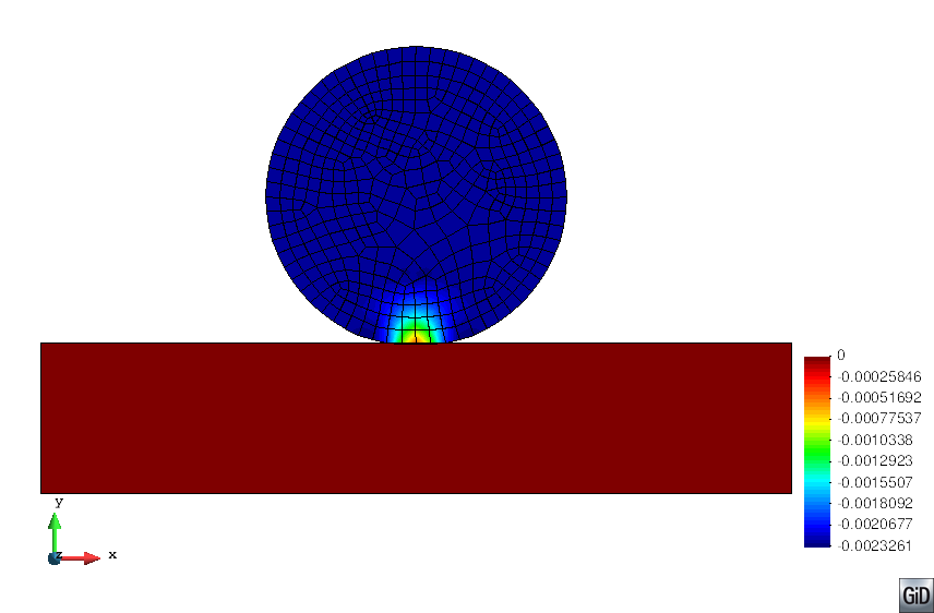
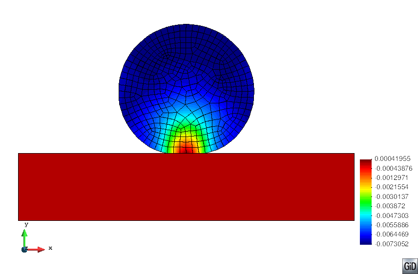
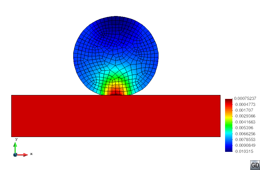
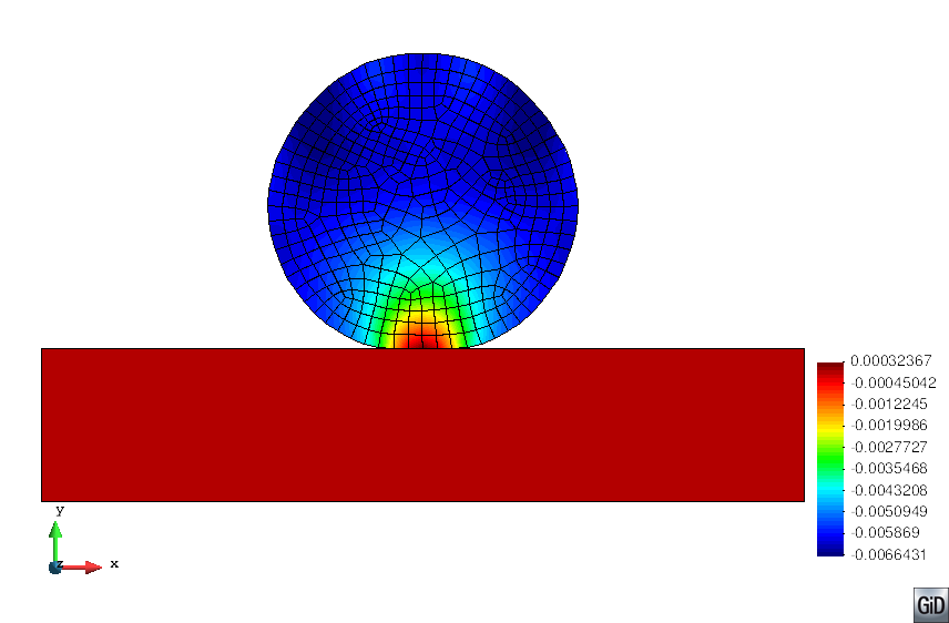
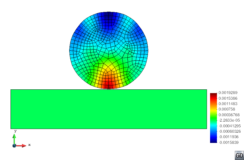
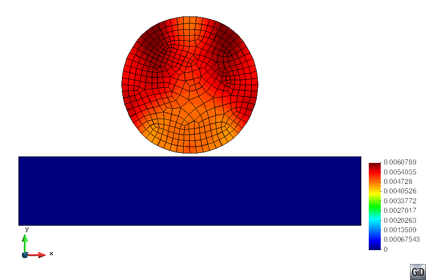
Figure 15: Vertical displacement field $u_{y}$ for the deformed geometry at $t=0$, $0.04$, $0.05$, $0.06$, $0.07$, $0.08$, $0.09$ and $0.1s$, respectively.

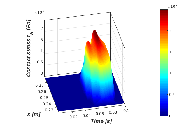
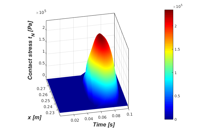
Figure 16: Contact stress distributions for $P=1$ and $P=2$. The stresses are much smoother for $P=2$ when compared with the oscillatory distribution for $P=1$.

Tables 17, 18 and 19 present the average numbers of CGGS iterations, average time per time step and speedup, respectively, using the standard modal Jacobi, the nodal Lagrange and the SDME bases. The best results were achieved for the SDME-H basis.

Table 17: Average number of CGGS iterations per time step. We observe that the SDME-H basis has the best performance

Order	Number of DOFs	Average number of CGGS iterations
		ST	Lagrange	SDME-M	SDME-H
1	962	27.74	19.68	-	-
2	3722	75.05	20.17	19.53	19.52
3	8282	64.47	19.04	21.57	20.20
4	14642	131.03	22.24	25.60	22.32
5	22802	129.05	25.38	27.61	22.52
6	32762	185.15	28.35	30.32	22.18
7	44522	199.64	30.94	31.07	22.99
8	58082	228.65	32.99	33.63	25.55
9	73442	270.68	35.95	34.88	28.10
10	90602	279.37	38.47	36.97	30.50

Table 18: Average time per time step using the CGGS method for the ST, Lagrange and SDME bases. We observe that the SDME-H basis has the best performance

Order	Number of DOFs	Average time for CGGS solution [s]
		ST	Lagrange	SDME-M	SDME-H
1	962	0.0073	0.0057	-	-
2	3722	0.0326	0.0112	0.0104	0.0104
3	8282	0.0623	0.0224	0.0247	0.0236
4	14642	0.2013	0.0436	0.0483	0.0437
5	22802	0.3034	0.0733	0.0783	0.0671
6	32762	0.6009	0.1127	0.1180	0.0933
7	44522	0.8590	0.1610	0.1610	0.1283
8	58082	1.2552	0.2156	0.2211	0.1784
9	73442	1.8583	0.2927	0.2866	0.2429
10	90602	2.3456	0.3850	0.3698	0.3183

Table 19: Speedup ratio for the computation time to solve the linear system of equations between the standard Jacobi basis and Lagrange basis and between the standard Jacobi basis and the minimum energy bases.

Order	Number of DOFs	Speedup
		Lagrange	SDME-M	SDME-H
1	962	1.28	-	-
2	3722	2.91	3.15	3.13
3	8282	2.78	2.52	2.64
4	14642	4.62	4.17	4.60
5	22802	4.14	3.87	4.52
6	32762	5.33	5.09	6.44
7	44522	5.33	5.33	6.69
8	58082	5.82	5.68	7.04
9	73442	6.35	6.48	7.65
10	90602	6.09	6.34	7.37

5.5 Three-dimensional cylinder impact problem

We present now the results for a frictionless impact of a hyperelastic cylinder on a plate, Fig. 17. The implicit Newmark time integration scheme was used. The convergence tolerances for the CGGS and Newton-Raphson procedures were both $10^{-6}$. The Schur complement was taken for the tangent stiffness matrix and the residue vector. The penalty parameter was $\epsilon_{N}=1.0\times 10^{4}$ and $\Delta\epsilon_{N}=1.0\times 10^{3}$. Large deformation was considered and the geometry and material properties are presented in Fig 17. We used $P+1$ Gauss-Legendre integration points for the contact elements. The tolerances for the gap function and contact stress were $10^{-3}$ and $10^{-2}$, respectively. The integration time is $T=0.2\,s$ and $\Delta t=10^{-3}\,s$. The initial conditions are $\mathbf{u}_{0}=\{0.000\;0.005\;0.000\}^{T}\,m$ and $\mathbf{v}_{0}=\{0.000\;-0.060\;0.000\}^{T}\,m/s$. The two faces of the plate in the $xy$-plane were completely fixed.

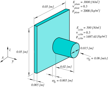
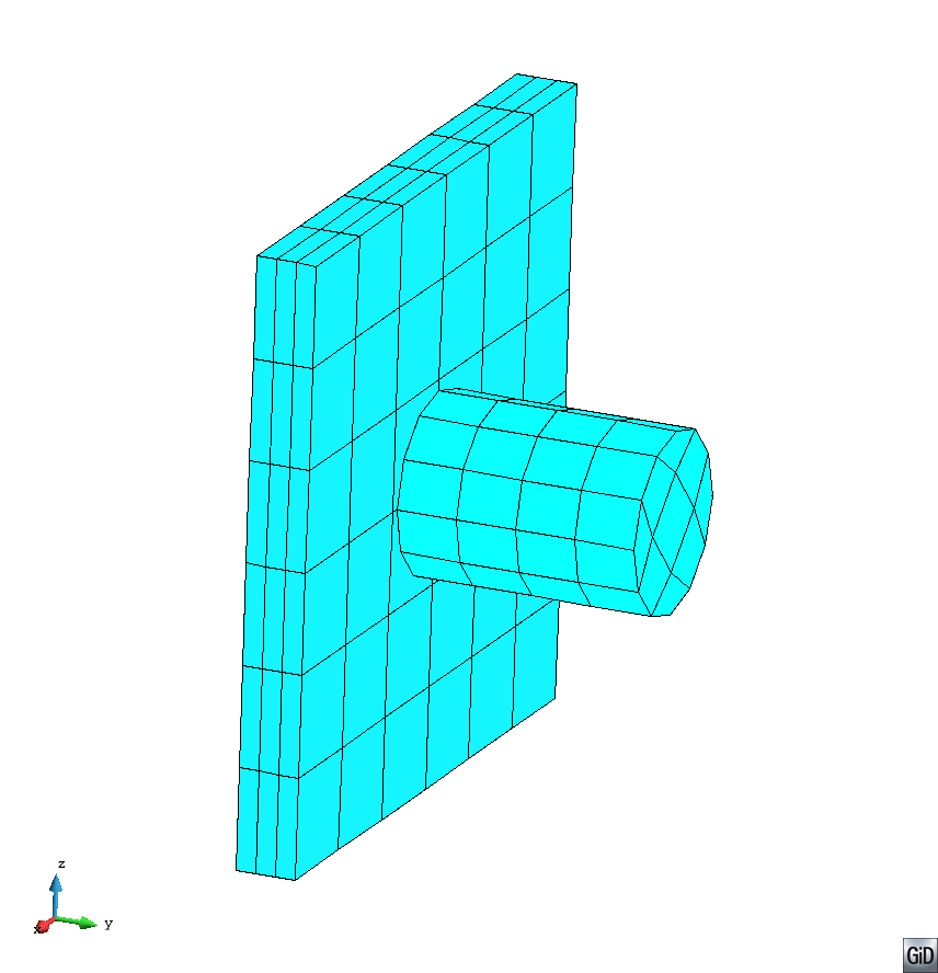
Figure 17: Domain geometry, material properties and initial conditions andesh of hexahedra for the cylinder impact problem.

Figure 18 shows the displacement field $u_{y}$ in the deformed structure at different time steps of the solution for interpolation order $P=3$.

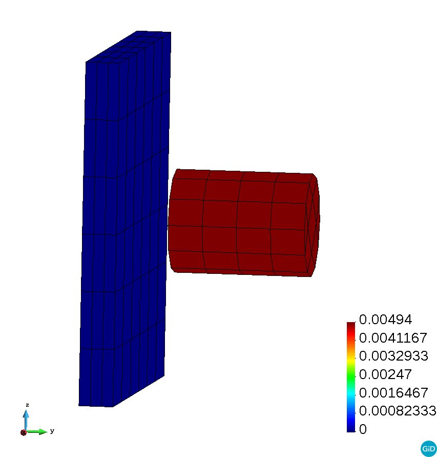
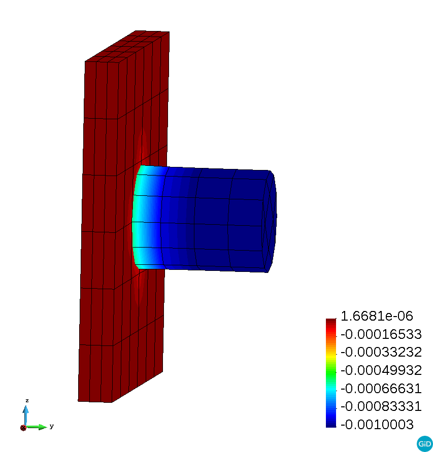
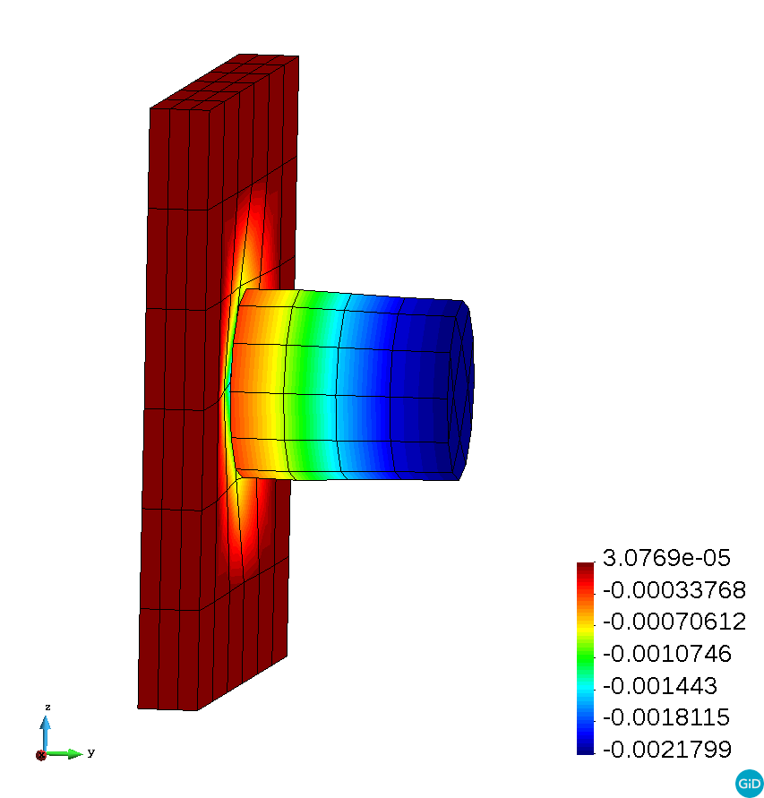
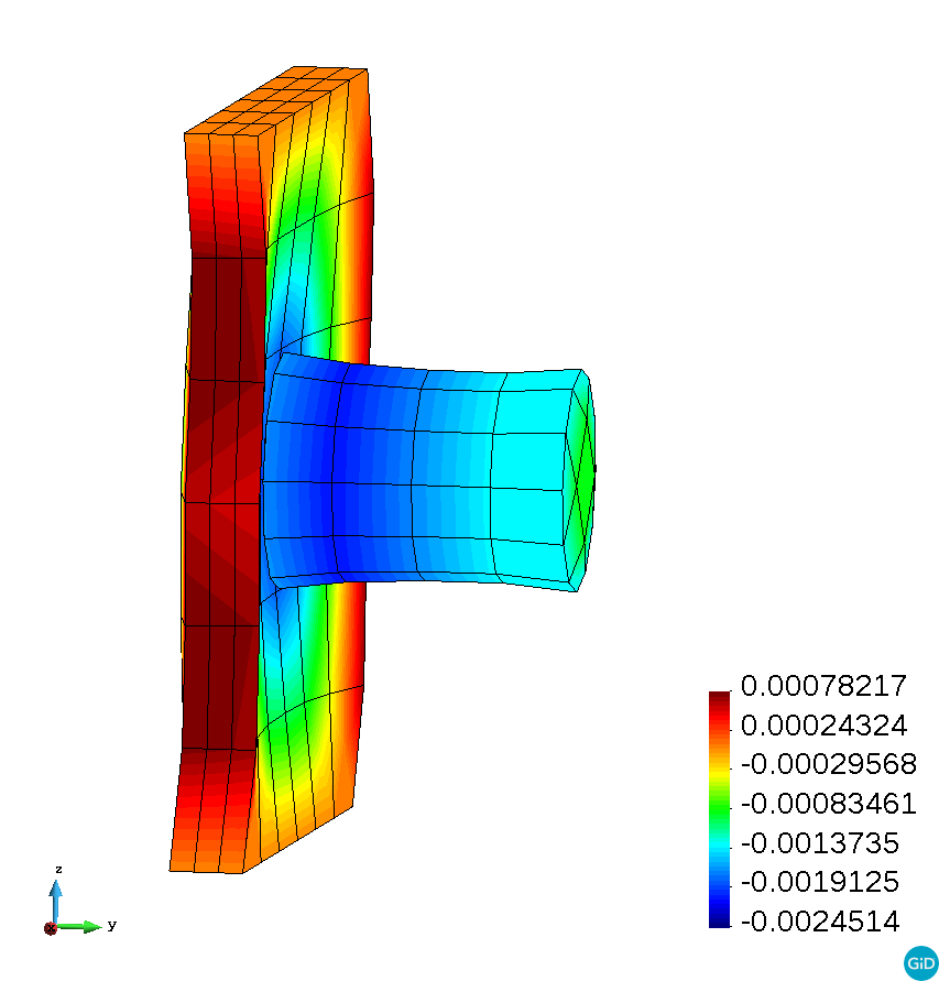
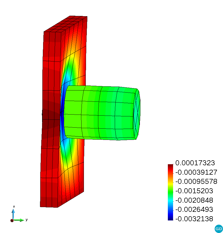
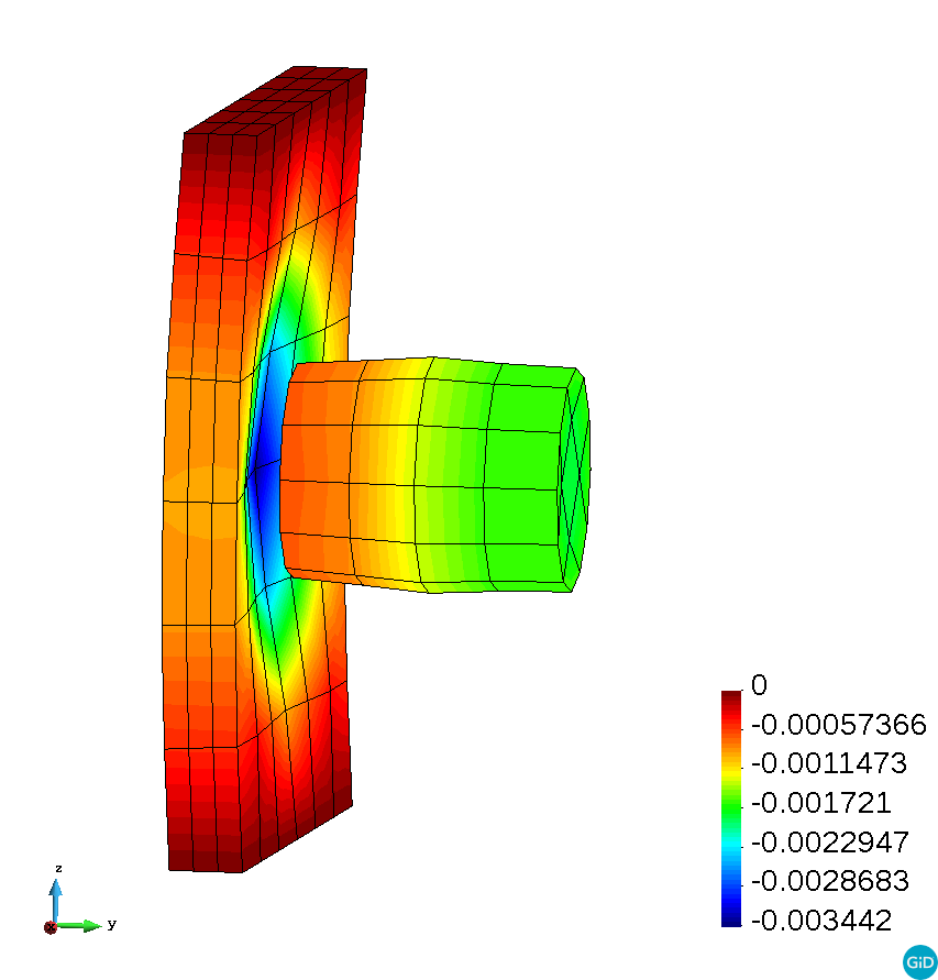
Figure 18: Displacement field $u_{y}$ for the deformed structure in $t=0$, $0.10$, $0.12$, $0.16$, $0.18$ and $0.20s$, respectively, for the cylinder impact problem.

Tables 20, 21 and 22 present the average numbers of CGGS iterations, average time per time step and speedup, respectively, using the standard modal Jacobi, the nodal Lagrange and SDME bases. The best results were achieved for the SDME-H basis.

Table 20: Average number of CGGS iterations per time step. The SDME-H basis performed better for all polynomial orders.

Order	Number of DOFs	Average number of CGGS iterations
		ST	Lagrange	SDME-M	SDME-H
1	652	27.55	27.64	-	-
2	4318	220.62	39.47	32.49	32.31
3	14299	169.56	37.67	35.15	31.78
4	31753	777.90	43.17	57.43	42.93
5	60922	785.29	50.28	52.15	41.32

Table 21: Average time per time step using the CGGS method for the ST, Lagrange and SDME bases. The SDME-H basis performed better for all polynomial orders.

Order	Number of DOFs	Average time for CGGS solution [s]
		ST	Lagrange	SDME-M	SDME-H
1	652	0.0092	0.0094	-	-
2	4318	0.4651	0.1085	0.0870	0.0866
3	14299	1.8288	0.4987	0.4446	0.4274
4	31753	24.7392	1.7316	2.2726	1.6837
5	60922	62.5139	4.9748	4.8295	4.0466

Table 22: Speedup ratio for the computation time to solve the linear system of equations between the standard Jacobi basis and Lagrange basis and between the standard Jacobi basis and the minimum energy bases.

Order	Number of DOFs	Speedup
		Lagrange	SDME-M	SDME-H
1	652	0.98	-	-
2	4318	4.29	5.35	5.37
3	14299	3.67	4.11	4.28
4	31753	14.29	10.89	14.69
5	60922	12.57	12.94	15.85

6 Conclusions

In this work, we applied high-order finite element bases to solve two and three-dimensional transient nonlinear structural and impact problems. The one-dimensional bases were constructed by performing simultaneous diagonalization of the internal modes and Schur complement of the boundary modes. Fabricated smooth solutions involving large displacements and strains were used to test the bases in static and transient (explicit and implicit) analyses.

The SDME bases performed significantly much better than the standard Jacobi basis for all nonlinear problems tested. For the static nonlinear test, the SDME-H basis had a better performance than the SDME-M basis for all polynomial orders when using the Gauss-Seidel preconditioner for the linear system solution. The same was observed when using the diagonal preconditioner for polynomial orders up to 6.

In the case of transient nonlinear problems with explicit time integration, the SDME-M basis had a speedup up of 27.7 when compared to the standard Jacobi basis. For the implicit time integration, the best results f or speedup were achieved by the SDME-M basis as well, with speedup up to 26.

For the conrod simulations, we observed that the SDME-H basis with the chosen set of parameters had a much better performance compared to the ST basis. Moreover, in the case of implicit time integration, there were less PCG iterations compared to the SDME-M basis for lower polynomial orders $(P<5)$. However, for higher polynomial orders, the number of PCG iterations significantly increase for the SDME-H basis, and the lowest number of iterations was achieved with the SDME-M basis.

The SDME-H basis had the best performance for the impact problems when compared to the standard Jacobi basis. For the two-dimensional disk impact problem, the SDME-H basis had better performance in the average by 13%, when compared to the nodal Lagrange basis with Gauss-Lobatto collocation points. For the higher polynomial orders ($P=5$ to $P=10$), the improvement was close to 22%. For the three-dimensional cylinder impact problem, the improvement for the same comparison and $P=5$ was close to 23%. When compared to the nodal Lagrange basis, the performance of the SDME-H was over 25% better.

The Gauss-Seidel preconditioner performed much better than the diagonal preconditioner in terms of the number of iterations for convergence for a given tolerance. However, it is difficult to implement it in an element wise fashion and requires the assemble of the global matrix. The diagonal preconditioner is simpler to implement in parallel without the need of the global matrix of the system of equations.

In general, the SDME bases had an outstanding performance when applied to non-linear structural problems including large deformation and strain and impact problems. For meshes with larger degrees of freedom, it is expected a better performance of the SDME bases.

References

- [1] G. E. Karniadakis, S. J. Sherwin, Spectral/hp Element Methods for Computational Fluid Dynamics, Oxford University Press, Oxford, 2005 (2005).
- [2] M. L. Bittencourt, Computational solid mechanics: variational formulation and high order approximation, 1st Edition, CRC Press, 2014 (2014).
- [3] I. Babuska, B. A. Szabó, I. N. Katz, The p-version of the finite element method, SIAM J. Numer. Anal. 18 (3) (1981) 515–545 (1981).
- [4] P. Carnevali, R. B. Morris, Y. Tsuji, G. Taylor, New basis functions and computational procedures for p-version finite element analysis, International Journal for Numerical Methods in Engineering 36 (1993) 3759–3779 (1993).
- [5] S. Adjerid, M. Aiffa, J. E. Flaherty, Hierarchical finite element bases for triangular and tetrahedral elements, Computer Methods in Applied Mechanics and Engineering 190 (2001) 2925–2941 (2001).
- [6] S. Beuchler, V. Pillwein, Sparse shape functions for tetrahedral p-fem using integrated jacobi polynomials, Computing 80 (2007) 345–375 (2007).
- [7] P. Šolín, T. Vejchodskỳ, Higher-order finite elements based on generalized eigenfunctions of the Laplacian, International Journal for Numerical Methods in Engineering 73 (10) (2008) 1374–1394 (2008).
- [8] M. L. Bittencourt, M. G. Vazquez, T. G. Vazquez, Construction of shape functions for the - and -versions of the fem using tensorial product, International Journal for Numerical Methods in Engineering 71 (2007) 529–563 (2007).
- [9] J. Shen, L. Wang, Fourierization of the Legendre–Galerkin method and a new space–time spectral method, Applied Numerical Mathematics 57 (5) (2007) 710–720 (2007).
- [10] J. P. Webb, R. Abouchacra, Hierarchical triangular elements using orthogonal polynomials, International Journal for Numerical Methods in Engineering 38 (1995) 245–257 (1995).
- [11] R. Abdul-Rahman, M. Kasper, Higher order triangular basis functions and solution performance of the cg method, Computer Methods in Applied Mechanics and Engineering 197 (2007) 115–127 (2007).
- [12] D. A. Castro, P. R. Devloo, A. M. Farias, S. M. Gomes, O. Durán, Hierarchical high order finite element bases for h(div) spaces based on curved meshes for two-dimensional regions or manifolds, Journal of Computational and Applied Mathematics 301 (2016) 241 – 258 (2016).
- [13] P. R. Devloo, O. Durán, S. M. Gomes, M. Ainsworth, High-order composite finite element exact sequences based on tetrahedral–hexahedral–prismatic–pyramidal partitions, Computer Methods in Applied Mechanics and Engineering 355 (2019) 952 – 975 (2019).
- [14] I. Babuska, B. Q. Guo, The h-p version of the finite element method for problems with nonhomogeneous essential boundary condition, Computer Methods in Applied Mechanics and Engineering 74 (1989) 1–28 (1989).
- [15] I. Babuska, A. Craig, J. Mandel, J. Pitkaranta, Efficient preconditioning for the p-version finite element method in two dimensions, SIAM Journal on Numerical Analysis 28 (3) (1991) 624–661 (1991).
- [16] J. Mandel, Hierarchical preconditioning and partial orthogonalization for the p-version finite element method, in: T. Chan, R. Glowinski, O. Windlund (Eds.), Proceedings of the 3th International Symposium on Domain Decomposition Methods for Partial Differential Equations, SIAM, Huston, Texas, 1990, pp. 141–156 (1990).
- [17] J. Mandel, On block diagonal and schur complement preconditioning, Numer. Math. 58 (1990) 79–93 (1990).
- [18] J. Mandel, An iterative solver for the p-version finite elements in three dimensions, Computer Methods in Applied Mechanics and Engineering 116 (1994) 175–183 (1994).
- [19] M. A. Casarin, Diagonal edge preconditioners in p-version and spectral element methods, SIAM J. Sci. Comput. 18 (2) (1997) 610–620 (1997).
- [20] V. G. Korneev, S. Jensen, Preconditioning of the p-version of the finite element method, Computer Methods in Applied Mechanics and Engineering 150 (1997) 215–238 (1997).
- [21] J. Mandel, Iterative solvers by substructuring for the p-version finite element method, Computer Methods in Applied Mechanics and Engineering 80 (1990) 117–128 (1990).
- [22] S. Jensen, V. Korneev, On domain decomposition preconditioning in the hierarchical p-version of the finite element method, Computer Methods in Applied Mechanics and Engineering 150 (1997) 215–238 (1997).
- [23] Y. Cai, Z. Bai, J. E. Pask, N. Sukumar, Hybrid preconditioning for iterative diagonalization of ill-conditioned generalized eigenvalue problems in electronic structure calculations, Journal of Computational Physics 255 (2013) 16–30 (2013).
- [24] F. de Prenter, C. V. Verhoosel, G. J. V. Zwieten, E. H. V. Brummelen, Condition number analysis and preconditioning of the finite cell method, Computer Methods in Applied Mechanics and Engineering 316 (2017) 297–327 (2017).
- [25] F. de Prenter, C. V. Verhoosel, E. H. V. Brummelen, Preconditioning immersed isogeometric finite element methods with application to flow problems, Computer Methods in Applied Mechanics and Engineering 348 (2019) 604–631 (2019).
- [26] K. Agathos, E. Chatzi, S. P. A. Bordas, A unified enrichment approach addressing blending and conditioning issues in enriched finite elements, Computer Methods in Applied Mechanics and Engineering 349 (2019) 673–700 (2019).
- [27] C. Rodrigues, M. L. Bittencourt, Construction of precondititioners by using high-order minimum energy basis, in: Proceedings of the 11th. World Congress on Computational Mechanics (WCCM XI), 2014 (2014).
- [28] L. de Bejar, K. Danielson, Critical time-step estimation for explicit integration of dynamics higher-order finite-element formulations, Journal of Engineering Mechanics 142 (7) (2016).
- [29] R. Browning, K. Danielson, M. Adley, Higher-order finite elements for lumped-mass explicit modeling of high-speed impacts, Journal of Impact Engineering 137 (2020).
- [30] K. T. Danielson, M. D. Adley, T. N. Williams, Second-order finite elements for hex-dominant explicit methods in nonlinear solid dynamics, Finite Elements in Analysis and Design 119 (2016) 63 – 77 (2016).
- [31] K. T. Danielson, Barlow’s method of superconvergence for higher-order finite elements and for transverse stresses in structural elements, Finite Elements in Analysis and Design 141 (2018) 84 – 95 (2018).
- [32] A. C. Nogueira Jr, M. L. Bittencourt, Spectral/hp finite elements applied to linear and non-linear structural elastic problems, Latin American Journal of Solids and Structures 4 (1) (2007) 61–85 (2007).
- [33] S. Dong, Z. Yosibash, A parallel spectral element method for dynamic three-dimensional nonlinear elasticity problems, Computers and Structures 87 (2009) 59–72 (2009).
- [34] C. F. Rodrigues, J. L. Suzuki, M. L. Bittencourt, Construction of minimum energy high-order helmholtz bases for structured elements, Journal of Computational Physics 306 (2016) 269–290 (2016).
- [35] Y. Yu, H. Baek, M. L. Bittencourt, G. E. Karniadakis, Mixed spectral/hp element formulation for nonlinear elasticity, Computer Methods in Applied Mechanics and Engineering 213-216 (0) (2012) 42 – 57 (2012).
- [36] J. L. Suzuki, M. L. Bittencourt, Application of the hp-fem for hyperelastic problems with isotropic damage, in: Computational Modeling, Optimization and Manufacturing Simulation of Advanced Engineering Materials, 2016, pp. 113–150 (2016).
- [37] J. L. Boldrini, E. A. B. de Moraes, L. R. Chiarelli, F. G. Fumes, M. L. Bittencourt, A non-isothermal thermodynamically consistent phase field framework for structural damage and fatigue, Computer Methods in Applied Mechanics and Engineering 312 (2016) 395–427 (2016).
- [38] L. R. Chiarelli, F. G. Fumes, E. A. B. de Moraes, G. A. Haveroth, J. L. Boldrini, M. L. Bittencourt, Comparison of high order finite element and discontinuous galerkin methods for phase field equations: Application to structural damage, Computers & Mathematics with Applications (2017).
- [39] G. A. Haveroth, E. A. Moraes, J. L. Boldrini, M. L. Bittencourt, Comparison of semi and fully-implicit time integration schemes applied to a damage and fatigue phase field model, Latin American Journal of Solids and Structures 15 (5) (2018).
- [40] A. Dias, A. Serpa, M. Bittencourt, High-order mortar-based element applied to nonlinear analysis of structural contact mechanics, Computer Methods in Applied Mechanics and Engineering 294 (2015) 19 – 55 (2015).
- [41] A. Dias, S. Proença, M. Bittencourt, High-order mortar-based contact element using nurbs for the mapping of contact curved surfaces, Computational Mechanics 64 (1) (2019) 85–112 (2019).
- [42] A. Akhavan-Safaei, S. H. Seyedi, M. Zayernouri, Anomalous features in internal cylinder flow instabilities subject to uncertain rotational effects, Physics of Fluids 32 (9) (2020) 094107 (2020).
- [43] X. Zheng, S. Dong, An eigen-based high-order expansion basis for structured spectral elements, Journal of Computational Physics 230 (23) (2011) 8573–8602 (2011).
- [44] J. Suzuki, Aspects of fractional-order modeling and efficient bases to simulate complex materials using finite element methods, Ph.D. thesis, University of Campinas (2017).
- [45] A. Laub, M. Heath, C. Paige, R. Ward, Computation of system balancing transformations and other applications of simultaneous diagonalization algorithms, IEEE Transactions on Automatic Control 32 (1987) 115–122 (1987).
- [46] B. C. Moore, Principal Component Analysis in Linear Systems: Controllability, Observability, and Model Reduction, IEEE Trans. Automatic Control AC-26 (1981) 17–32 (1981).
- [47] C. Canuto, M. Youssuff Hussaini, A. Quarteron, Z. T.A., Spectral Methods – Fundamentals in Single Domains, Springer, 2006 (2006).
- [48] K. J. Bathe, Finite Element Procedures in Engineering Analysis, Prentice-Hall, New Jersey, 1982 (1982).
- [49] J. Bonet, R. D. Wood, Nonlinear continuum mechanics for finite element analysis, 2nd Edition, Cambridge, 2008 (2008).
- [50] P. Wriggers, Nonlinear Finite Element Methods, Springer, 2008 (2008).
- [51] A. P. C. Dias, Numerical simulation of structural contact problems with high-order mortar-based element, Ph.D. thesis, Department of Integrated Systems, School of Mechanical Engineering, University of Campinas, Campinas - Brazil (2017).
- [52] A. P. C. Dias, S. P. B. Proenca, M. L. Bittencourt, Advances in Computational Coupling and Contact Mechanics: Chapter 2-Standard and Generalized High-order Mortar-based Finite Elements in Computational Contact Mechanics, 1st Edition, Vol. 1, World Scientific (EUROPE), London, UK, 2018 (2018).
- [53] O. Axelsson, Iterative Solution Methods, Cambridge University Press, 1994 (1994).
- [54] H. B. Khenous, P. Laborde, Y. Renard, Mass redistribution method for finite element contact problems in elastodynamics, European Journal of Mechanics A/Solids 27 (2008) 918–932 (2008).