Robust Classification via Support Vector Machines

Abstract

Classification models are very sensitive to data uncertainty, and finding robust classifiers that are less sensitive to data uncertainty has raised great interest in the machine learning literature. This paper aims to construct robust Support Vector Machine classifiers under feature data uncertainty via two probabilistic arguments. The first classifier, Single Perturbation, reduces the local effect of data uncertainty with respect to one given feature and acts as a local test that could confirm or refute the presence of significant data uncertainty for that particular feature. The second classifier, Extreme Empirical Loss, aims to reduce the aggregate effect of data uncertainty with respect to all features, which is possible via a trade-off between the number of prediction model violations and the size of these violations. Both methodologies are computationally efficient and our extensive numerical investigation highlights the advantages and possible limitations of the two robust classifiers on synthetic and real-life data.

1 Introduction

A prediction model is said to be robust if small changes in the data would not change the model outputs, which is a consistent interpretation of robust prediction modeling across the theoretical statistics and computational robustness literature. Standard practical approaches to achieve robust predictions in the machine learning literature include outlier detection, testing prediction performance under data contamination or allowing for data uncertainty (DU) in the prediction model.

Creating robust prediction models is imperative whenever the current and/or future data are affected by DU. Specifically, DU means that the data are affected by i) sampling error, ii) ambiguity or iii) data noise, and each source of DU affects the robustness of the prediction model. Sampling error is inevitable, and this source of DU is negligible in large samples, which is often the case in machine learning modeling. Data ambiguity goes beyond missing data, and is a challenging issue that often occurs in categorical data. For example, insurance fraud data contain information about the event leading to a claim (major/minor) that is very subjective; similarly, likert scale features in automatized hiring processes are influenced by ambiguous questionnaires. Data noise is the unexplained variability within the observational data. The data noise could be associated with the features or response variable(s) in supervised learning. In summary, data ambiguity and feature and/or label noise are the important sources of DU, though data noise is the main source of DU considered in the robust classification literature.

Support vector machine (SVM) is an effective classifier with a variety of real-world applications. However, SVM is very sensitive to label and feature noise, and thus, a large amount of work has been done to robustify SVM against such sources of DU. For example, prior studies have dealt with allocating different weights to individual data points to reduce the effect of outliers (Wu and Liu, 2013; Yang et al., 2007); various loss functions have been used to robustify SVM predictions with respect to feature noise (Bamakan et al., 2017; Brooks, 2011; Huang et al., 2014; Shen et al., 2017; Singh et al., 2014; Suykens and Vandewalle, 1999; Wu and Liu, 2007); standard approaches have also been explored in the field of robust optimization (RO), such as metric-type (non-probabilistic) uncertainty sets (Bertsimas et al., 2018; Bi and Zhang, 2005; Trafalis and Gilbert, 2006; Xu et al., 2009); another RO approach, namely, chance constraints (CC) that are probabilistic uncertainty sets, has been introduced in the literature so that the underlying optimization problems used in SVM prediction exhibit more robust outputs whenever DU is present (Huang et al., 2012; Lanckriet et al., 2002; Wang et al., 2018), though a wider discussion of SVM modeling with CC is available in Ben-Tal et al. (2011). It is evident – even from this short introduction – that Operational Research (OR) has been a key ingredient in supervised and unsupervised learning, and an excellent review in this sense is available in Gambella et al. (2021).

The main purpose of this paper is to reduce the effect of feature noise for binary SVM classifiers. We explore the internal structure of the classical SVM (C-SVM) classifier in order to detect and tackle the feature noise via probabilistic arguments, while the eventual label noise issue is put aside in this paper, since our proposed probabilistic arguments are not easily extendable to prediction modeling under label noise.

The first proposed robust SVM classifier is the Single Perturbation (SP-SVM), and aims to reduce the local effect of DU with respect to one given feature by embedding this possible source of uncertainty into the prediction model. This technique is very popular in RO, where the so-called CCs are constructed to replace its non-robust counterparts (that are assumed to be certain). SP-SVM is an effective classifier whenever DU is present, and it could be used to test whether or not each feature is affected by DU.

The second proposed robust SVM classifier is the Extreme Empirical Loss (EEL-SVM), and aims to reduce the aggregate effect of DU. This is achieved by introducing a trade-off between the number of prediction model violations (misclassifications) and the size of these violations, which is explained via a probabilistic argument. Simply speaking, C-SVM assigns the same importance (probability) to each misclassification and aims to reduce the overall prediction error. In contrast, EEL-SVM focuses only on the most significant errors, i.e. the extreme errors, which increases the accuracy around the borderline decisions and improves the model accuracy. This approach is inspired by the standard risk measure, namely, Conditional Value-at-Risk, which was shown to be very robust in the context of model ambiguity modeled via RO (Asimit et al., 2017).

C-SVM is a special case of both SP-SVM and EEL-SVM, and thus, our robust formulations generalize C-SVM. Efficient convex quadratic programming solvers are used for solving SP-SVM and EEL-SVM, but the computational times of SP-SVM and EEL-SVM are not smaller than C-SVM, and this effect is known in the RO literature as the price of robustness. Note that, due to its sparsity, EEL-SVM has a lower computational time than SP-SVM and the reduction in computational time is mainly influenced by the sample size. Our numerical experiments have shown that both SP-SVM and EEL-SVM perform very well when compared with their robust SVM competitors. Moreover, even though the overall performance of SP-SVM is slightly superior to EEL-SVM, the sparsity trait of EEL-SVM is extremely appealing from the computational perspective; for specific details about our numerical experiments, see Section 4.

It is worth noting that, unlike the existing methods based on CC  (Ben-Tal et al., 2011; Huang et al., 2012; Lanckriet et al., 2002; Wang et al., 2018), SP-SVM does not require estimating the covariance matrix, which is not always computationally stable  (Fan et al., 2016; Ledoit and Wolf, 2020). Moreover, in this paper, we only provide explicit derivations for SP-SVM and EEL-SVM with the most popular loss function, i.e. Hinge loss, but similar derivations are possible for any other loss function. In addition to the two new robust SVM models, we also prove Fisher consistency for a general convex loss function and binary SVM classifier.

The paper is organized as follows. Section 2 provides the necessary background, while Section 3 illustrates the two proposed robust SVM classifiers. Section 4 summarizes our numerical experiments conducted over synthetic and real-life datasets. Section 5 includes some final comments and recommendations that emerge from our paper. All proofs are relegated to the appendix.

2 Background and Problem Definition

The current section takes stock of the necessary background related to binary SVM classification. Section 2.1 briefly explains the C-SVM formulation, while Section 2.2 provides a comprehensive description of the pros and cons of various loss functions which is a pivotal choice for any SVM implementation. Finally, Section 2.3 discusses the importance of Fisher consistency property in classification followed by a theoretical contribution in the context of binary classification, which is stated as Theorem 1.

2.1 Problem Definition

Our starting point is the training set that contains $N$ instances and their associated labels, $\{(\mathbf{x}_{i},y_{i}),\;i=1,\ldots,N\}$, where $\mathbf{x}_{i}\!\in\!\mathcal{X}\!\subseteq\!\mathbb{R}^{d}$ and $y_{i}\!\in\!\mathcal{Y}$. The training set is assumed to be sampled from $(X,Y)$, but the binary classification reduces to $\mathcal{Y}:=\{-1,1\}$, where $y_{i}=1$ if $\mathbf{x}_{i}$ is in the positive class, $\mathcal{C}_{+1}$, and $y_{i}=-1$ if $\mathbf{x}_{i}$ is in the negative class, $\mathcal{C}_{-1}$. The main objective is to construct an accurate (binary) classifier $c:\mathcal{X}\rightarrow\mathcal{Y}$ which maximizes the probability that $c\big{(}\mathbf{x}_{i}\big{)}=y_{i}$.

SVM aims to identify a separation hyper-plane $\mathbf{w}^{T}\phi\big{(}\mathbf{x}\big{)}+b$ that generates two parallel supporting hyper-planes:

$$\mathbf{w}^{T}\phi\big{(}\mathbf{x}\big{)}+b=1\quad\mbox{and}\quad\mathbf{w}^{T}\phi\big{(}\mathbf{x}\big{)}+b=-1,$$ (2.1)

where $\phi(\cdot)$ is a notional function that transforms the feature space into a synthetic feature space that allows a linear hyper-plane separation of the data (when linear classifiers are not effective on the original data). The data are rarely perfectly separable, and a compromise is made by allowing classification violations for the non-separable data. The latter is also known as soft-margin SVM and is formulated as follows:

$$\underset{\mathbf{w},b}{\text{min}}\;\frac{1}{2}\mathbf{w}^{T}\mathbf{w}+C\displaystyle\sum_{i=1}^{N}L(1-y_{i}(\mathbf{w}^{T}\phi(\mathbf{x}_{i})+b)).$$ (2.2)

The first term aims to find the ‘best’ classifier by maximizing the distance between the two hyper-planes defined in (2.1), while the second term penalizes the classifier’s violations measured via a given loss function $L:\mathbb{R}\rightarrow\mathbb{R}_{+}$; for details, see Vapnik (2000).

2.2 Loss Function

Solving the general SVM formulation in (2.2) requires specific solvers that depend upon the loss function choice, which has a central role in SVM classification. The existing literature has dealt with numerous piecewise loss functions, and a summary is given below:

1. Hinge loss: $L_{H}(u):=\max\{0,u\}$;

2. Truncated Hinge loss ($a\geq 1$): $L_{TH}(u):=\min\{\max\{0,u\},a\}$;

3. Pinball loss ($a\leq 0$): $L_{P}(u):=\max\{au,u\}$;

4. Pinball loss with ‘$\epsilon$ zone’ ($\epsilon\geq 0$ and $a,b\leq 0$): $L_{PEZ}(u):=\max\{0,u-\epsilon,au+b\}$;

5. Truncated Pinball loss ($a\leq 0$ and $b\geq 0$): $L_{TP}(u):=\max\{u,\min\{au,b\}\}$.

The standard choice, $L_{H}$, leads to efficient computations as it reduces (2.2) to solving a convex Linearly Constrained Quadratic Program (LCQP), which is the original SVM formulation as explained in Vapnik (2000). Moreover, the Hinge loss is proved to be an upper bound of the classification error (Zhang, 2004; Shen et al., 2017), therefore it is a pivotal loss choice. At the same time, the Hinge loss has been criticized for not being robust and extremely sensitive to outliers, whereas the Truncated Hinge loss proposed by Wu and Liu (2007) overcomes this issue at the expense of computational complexity. The lack of convexity of this loss function requires a bespoke algorithm, namely, the Difference of Convex Functions Optimization Algorithm (DCA), which is computationally less efficient than standard LCQP solvers used for solving C-SVM and our proposed robust formulations (SP-SVM and EEL-SVM). The optimization problems based on the two Pinball losses require solving LCQPs with many more linear equality constraints than the Hinge loss, but the Pinball loss seems to be more robust and stable when re-sampling (Huang et al., 2014). Similar arguments have been used in Shen et al. (2017) to justify that the Truncated Pinball loss is a good choice when dealing with feature noise, though it shares the same computational shortcoming with the Truncated Hinge loss, that is, it requires non-convex solvers.

All previous five loss functions are piecewise linear, which is a computational advantage, but non-piecewise linear loss functions have been proposed in the existing literature. For example, the Least Square loss with $L_{LS}(u):=u^{2}$ is considered in Suykens and Vandewalle (1999) for which an efficient LCQP formulation is proposed; the Correntropy loss is defined in Singh et al. (2014), but variants of this have been investigated (see Xu et al., 2017 for SVM-like formulations). One could understand the possible advantages of non-linear convex loss functions for other classification methods from Lin (2004), where the Hinge loss is shown to be the tightest margin-based upper bound of the misclassification loss for many well-known classifiers. Further, it is numerically shown that this property does not suffice to think of the Hinge loss as the universally ‘best’ choice to measure misclassification. Strictly convex loss functions are argued in Bartlett et al. (2006) to possess appealing statistical properties when studying misclassification.

Even though the loss function is a pivotal choice in SVM classification, our two new robust classifiers are not restricted to a specific loss function, and thus, SP-SVM and EEL-SVM formulations are quite general and introduce two new methodologies of tackling binary classification in the presence of DU. However, the SP-SVM (instance (3.2)) and EEL-SVM (instance (3.7)) illustrations of this paper are only focused on Hinge loss formulations, though any other illustrations are possible. Therefore, the robustness of SP-SVM and EEL-SVM is a result of how these classifiers deal with DU, and not a by-product of choosing the ‘best’ loss function.

2.3 Fisher Consistency

A desirable loss function property for a generic classifier is Fisher consistency or classification calibration (Bartlett et al., 2006). By definition, the loss function $L$ is Fisher consistent if

$$\operatorname*{arg\,min}_{f:\mathcal{X}\rightarrow\mathbb{R}}\mathbf{E}_{\mathcal{X},\mathcal{Y}}L\big{(}1-Yf(\mathbf{X})\big{)}$$ (2.3)

is solved by the Bayes classifier that is defined as follows:

$$f_{Bayes}^{\ast}(\mathbf{x})=\left\{\begin{array}[]{rll}1,&\quad\text{if}&\Pr(Y=1|\mathbf{x})>\Pr(Y=-1|\mathbf{x}),\\ -1,&\quad\text{if}&\Pr(Y=1|\mathbf{x})<\Pr(Y=-1|\mathbf{x}).\end{array}\right.$$

In the context of binary SVM classification, one could show that (2.3) holds if

$$\operatorname*{arg\,min}_{z\in\mathbb{R}}\mathbf{E}_{\mathcal{Y}|\textbf{x}}L(1-Yz)=f_{Bayes}^{*}(\mathbf{x})$$ (2.4)

is true for all $\mathbf{x}\in\mathcal{X}$; e.g., see Proposition 1 in Wu and Liu (2007).

Fisher consistency has been extensively investigated in the literature, and we now provide a concise review that relates to our framework. Theorem 3.1 in Lin (2004) shows that, if the global minimizer of (2.3) exists, then it has to be the same as the Bayes decision rule, which is valid for any classification method. In the binary SVM setting, Proposition 1 in Wu and Liu (2007) and Theorem 1 in Shen et al. (2017) show that this property also holds for non-convex loss functions; the first result covers a large set of truncated loss functions, whereas the second focuses on the Truncated Pinball loss. Lemma 3.1 of Lin (2002) shows that the Hinge loss is Fisher consistent, and Theorem 1 in Huang et al. (2014) shows the same for the (convex loss) Pinball loss. Our next result extends Fisher consistency to a general convex loss function $L$ for the binary SVM case, and its proof is relegated to Appendix A.1.1.

Theorem 1.

Assume that $L:\mathbb{R}\to\mathbb{R}_{+}$ is a convex loss function such that $L(0)=0$. If $L(\cdot)$ is linear on $(0,2+\epsilon)$ for some $\epsilon>0$, then $L$ is Fisher consistent.

3 Robust SVM

This section explains the concept of robust SVM in a more formal way and provides the technical details for our two robust SVM; that is, SP-SVM in Section 3.1, and EEL-SVM in Section 3.2. Finally, a summary of practical recommendations when using our robust SVM formulations is given in Section 3.3.

3.1 Single Perturbation SVM

SP-SVM aims to reduce the local effect of DU with respect to one given feature by embedding this possible source of uncertainty into the optimization problem that describes our robust prediction model. The main idea is the appropriation of a standard RO approach that relies on CCs constructed to replace its non-robust counterparts (assumed to hold almost surely). That is, SP-SVM extends C-SVM by adjusting the feasibility set through parameter $\alpha$ that controls the DU level; $\alpha$ is tuned like in any other hyper-parameter model.

Previous robust SVM classifiers that rely on CC require the covariance (feature) matrix estimate, which is computable but brings some practical drawbacks; the empirical covariance matrix is computationally unstable when $d$ is large, and is often not positive semi-definite if missing values are present in the sample. This is not the case for SP-SVM, whose robustness is achieved by identifying the feature affected the most by DU. We choose this feature as the one with the highest variance whenever data are less interpretable (see Sections 4.1 and 4.2), though domain knowledge could help with choosing this feature (see Section 4.3).

Solving (2.2) under the Hinge loss is equivalent to solving the following LCQP instance:

$$\underset{\mathbf{w},b,\bm{\xi}}{\text{min}}\;\;\frac{1}{2}\mathbf{w}^{T}\mathbf{w}\!+\!C\displaystyle\sum_{i=1}^{N}\xi_{i}$$ (3.1)

$$\;\text{s.t.}\;\;y_{i}\big{(}\mathbf{w}^{T}\phi(\mathbf{x}_{i})\!+\!b\big{)}\geq 1\!-\!\xi_{i},\;\xi_{i}\geq 0,\;\;1\leq i\leq N,$$

where $C>0$ is a penalty constant that becomes a tuning parameter in the actual implementation phase. Equation (3.1) represents the mathematical formulation of C-SVM.

We are interested in calibrating (3.1) in the presence of DU with respect to one feature, e.g., the $k^{th}$ feature. Thus, the $j^{th}$ entry of $\phi\big{(}\mathbf{x}_{i}\big{)}$, denoted by $\phi_{j}\big{(}\mathbf{x}_{i}\big{)}$, is deterministic for all $1\leq i\leq N$ and $1\leq j\neq k\leq d$, whereas the $k^{th}$ feature is affected by an error term $Z_{ik}$, hence $\phi_{k}\big{(}\mathbf{x}_{i}\big{)}$ is replaced by $\phi_{k}\big{(}\mathbf{x}_{i}\big{)}+Z_{ik}$ for all $1\leq i\leq N$. Moreover, each error term is defined on a probability space $(\Omega_{ik},\mathcal{F},P)$ with $\Omega_{ik}\subseteq\mathbb{R}$. Therefore, the DU variant of (3.1) with respect to the $k^{th}$ feature becomes

$$\underset{\mathbf{w},b,\bm{\xi}}{\text{min}}\;\;\frac{1}{2}\mathbf{w}^{T}\mathbf{w}+C\displaystyle\sum_{i=1}^{N}\xi_{i}$$ (3.2)

$$\;\text{s.t.}\;\;\Pr\bigg{(}y_{i}\Big{(}\mathbf{w}^{T}\phi\big{(}\mathbf{x}_{i}\big{)}+w_{k}Z_{ik}+b\Big{)}\geq 1-\xi_{i}\bigg{)}\geq\alpha,\;\xi_{i}\geq 0,\;1\leq i\leq N,$$

where $\alpha\in[0,1]$ reflects the unknown modeler’s perception of DU that is later tuned. This kind of probability-like constraint is also known as CC in the OR literature.

For any given tuple $(i,k)$, the cumulative distribution function (cdf) of $Z_{ik}$, $F_{ik}(\cdot)$, is defined on $\Omega_{ik}$. Furthermore, we define two generalized inverse functions as follows:

$$F_{ik}^{-1}(t):=\inf\big{\{}x\in\mathbb{R}:\;F_{ik}(x)\geq t\big{\}}\quad\text{and}\quad F_{ik}^{-1+}(t):=\sup\big{\{}x\in\mathbb{R}:\;F_{ik}(x)\leq t\big{\}}$$

for all $t\in[0,1]$, where $\inf\varnothing=\infty$ and $\sup\varnothing=-\infty$ hold by convention. Clearly,

$$t\leq\Pr\big{(}Z_{ik}\leq x\big{)}\Leftrightarrow F_{ik}^{-1}(t)\leq x\quad\text{and}\quad\Pr\big{(}Z_{ik}<\!x\big{)}\!\leq t\Leftrightarrow x\leq F_{ik}^{-1+}(t),\;\;x\in\mathbb{R}\;\text{and}\;t\in[0,1].$$

Therefore, the CC from (3.2) is equivalent to

$$y_{i}\big{(}\mathbf{w}^{T}\phi(\mathbf{x}_{i})+b\big{)}+y_{i}w_{k}F_{ik}^{-1+}(1\!-\!\alpha)\geq 1\!-\!\xi_{i},\;\;y_{i}\big{(}\mathbf{w}^{T}\phi(\mathbf{x}_{i})+b\big{)}+y_{i}w_{k}F_{ik}^{-1}(\alpha)\geq 1\!-\!\xi_{i}$$ (3.3)

when $y_{i}w_{k}\geq 0$ or $y_{i}w_{k}<0$, respectively. Without imposing any restriction on $F_{ik}$, the conditional constraint from (3.3) makes (3.2) a mixed integer programming instance, which is a major computational shortcoming for large scale problems. The next set of conditions enable us to solve (3.2) efficiently.

Assumption 3.1.

$F_{ik}^{-1}(\alpha)+F_{ik}^{-1+}(1-\alpha)=0$ for a given integer $1\leq k\leq d$ and some $\alpha\in[0,1]$.

If the random error $Z_{ik}$ is defined on $\Omega_{ik}=\big{(}-\omega_{ik},\omega_{ik}\big{)}$ with $0<\omega_{ik}\leq\infty$ such that its cdf is continuous and increasing, and $F_{ik}(\cdot)+F_{ik}(-\cdot)=1$ in a neighborhood of $F_{ik}^{-1+}(\alpha)$, then Assumption 3.1 holds. Note that symmetric and continuous cdf, such as Gaussian, Student’s $t$ or any other member of the elliptical family of distributions centered at $0$ satisfies Assumption 3.1; for details, see Fang et al. (1990). Therefore, Assumption 3.1 is quite general.

Under Assumption 3.1, (3.3) is equivalent to

$$y_{i}\big{(}\mathbf{w}^{T}\phi(\mathbf{x}_{i})+b\big{)}-|w_{k}|F_{ik}^{-1}(\alpha)\geq 1-\xi_{i},$$

and in turn, (3.2) is equivalent to solving

$$\begin{array}[]{llc}\underset{\mathbf{w},b,\bm{\xi}}{\text{min}}&\frac{1}{2}\mathbf{w}^{T}\mathbf{w}+C\displaystyle\sum_{i=1}^{N}\xi_{i}&\\ \;\text{s.t.}&y_{i}\big{(}\mathbf{w}^{T}\phi(\mathbf{x}_{i})+b\big{)}\geq 1\!-\!\xi_{i}&(i)\\ &y_{i}\big{(}\mathbf{w}^{T}\phi(\mathbf{x}_{i})+b\big{)}-y_{i}w_{k}a_{ik}\geq 1\!-\!\xi_{i}&(ii)\\ &y_{i}\big{(}\mathbf{w}^{T}\phi(\mathbf{x}_{i})+b\big{)}+y_{i}w_{k}a_{ik}\geq 1\!-\!\xi_{i}&(iii)\\ &\xi_{i}\geq 0,\;\;1\leq i\leq N,&(iv)\end{array}$$ (3.4)

where $a_{ik}:=F_{ik}^{-1}(\alpha)$. If $a_{ik}\leq 0$ for all $1\leq i\leq N$, then the inequality constraints (3.4) (ii) and (iii) are redundant, and thus, SP-SVM and SVM are identical, i.e. the $k^{th}$ feature is not affected by DU. If $a_{ik}\geq 0$ for all $1\leq i\leq N$, then the inequality constraint (3.4) (i) is redundant and the $k^{th}$ feature is affected by DU, in which case SP-SVM becomes more conservative than SVM, i.e. the SP-SVM hyper-plane violations $\xi_{i}$’s are allowed to be larger (than the C-SVM violations) due to DU.

We now provide a practical recommendation to finding a ‘reasonable’ choice for $a_{ik}$. One possibility is to assume a Gaussian random noise with zero mean and variance equal to the sampling error estimate, i.e.

$$a_{ik}=\hat{a}_{k}:=q_{\alpha,G}\sqrt{\frac{1}{N\!-\!1}\displaystyle\sum_{i=1}^{N}(x_{ik}-\bar{x}_{k})^{2}}\;\mbox{and}\;\bar{x}_{k}:=\frac{1}{N}\sum_{i=1}^{N}x_{ik}\quad\text{for all $1\leq i\leq N$},$$

where $q_{\alpha,G}$ is the $\alpha$-Normal quantile. It could be argued that the Gaussian random noise might underestimate DU, hence a more heavy-tailed noise, such as Student’s $t$, might be more appropriate; in that case, we could simply replace $q_{\alpha,G}$ by the $\alpha$-quantile of the distribution of choice. We always tune $\alpha$ for values greater than $0.5$, i.e. $a_{ik}>0$ for all $1\leq i\leq N$, since DU is assumed to be present. Therefore, our SP-SVM implementations require solving LCQP instances with $3N$ inequality constraints, though C-SVM implementations require solving LCQP instances with $2N$ inequality constraints; this is not surprising and is known as the price of robustness in the OR literature. An explicit solution for (3.4) is detailed in Appendix A.1.2, where we do not make any assumption on the sign of $a_{ik}$’s.

3.2 Extreme Empirical Loss SVM

EEL-SVM is designed to reduce the overall effect of DU with respect to all features that are possibly affected by random noise, which is different from SP-SVM where only one feature is assumed to be affected by noise. This does not mean that EEL-SVM is ‘better’ than SP-SVM, as the two approaches complement each other, and Section 4 provides empirical evidence in that sense.

Simply speaking, EEL-SVM creates a trade-off between the number of model misclassifications and the size of these violations, which is explained via a probabilistic argument. While C-SVM assigns the same importance (probability) to each $\xi_{i}$, i.e. $1/N$, so that the overall prediction error is minimized, EEL-SVM considers that only some of the largest individual model violations affect the overall classification error. This means that EEL-SVM robustifies the classifier by paying particular attention to outliers without removing such data points that go astray from the general trend, since such sub-samples may not be a negligible portion of the data when DU is present.

The soft-margin SVM from (2.2) could be rewritten as

$$\underset{\mathbf{w},b}{\text{min}}\;\frac{1}{2}\mathbf{w}^{T}\mathbf{w}+C\widehat{E}\Big{[}L\Big{(}1-Y\big{(}\mathbf{w}^{T}\phi\big{(}\mathbf{X}\big{)}+b\big{)}\Big{)}\Big{]},$$ (3.5)

where the second term acts as the empirical estimate of the penalty associated with the classifier’s violations; this is given by the average model deviation measured via the loss function $L$. The loss function choice could influence the borderline decisions where examples could be classified either way, and thus, a ‘good’ loss choice may reduce the misclassification error. Many SVM classifiers focus on the choice of $L$, though the penalty term is always based on the usual sample average with equal importance to all hyper-plane violations. EEL-SVM aims to focus more on the large deviations that may considerably perturb the classification decision in the presence of DU. To this end, we place more weight to the larger violations via a novel empirical penalty function, namely, the Extreme Empirical Loss (EEL), which is formulated as

$$\min_{z}z\!+\!\frac{1}{N(1\!-\!\alpha)}\sum_{i=1}^{N}\max\big{\{}\zeta_{i}\!-\!z,0\big{\}},$$ (3.6)

where $\zeta_{i}=L\big{(}1-y_{i}(\mathbf{w}^{T}\phi(\mathbf{x}_{i})\!+\!b)\big{)}$ are the individual model violations. Note that (3.6) is the empirical estimate of the Conditional Value-at-Risk at level $\alpha$ ($CVaR_{\alpha}$) of the classifier’s violations, i.e.

$$\widehat{CVaR}_{\alpha}\Big{(}L\big{(}1-Y(\mathbf{w}^{T}\phi(\mathbf{X})+b)\big{)}\Big{)}.$$

For details, see the seminal paper Rockafellar and Uryasev (2000) which introduces $CVaR$, a well-known risk management measure. The parameter $0\leq\alpha<1$ represents the caution level chosen by the modeler; a higher value of $\alpha$ would penalize fewer extreme violations, i.e. large $\xi_{i}$’s. This is made obvious by noting that (3.6) is equivalent to

$$\frac{1}{r}\sum_{i=1}^{r}\zeta_{i,N}\;\mbox{if}\;\alpha=1-\frac{r}{N},\;1\leq r\leq N$$

for any integer $r$, where $\zeta_{1,N}\geq\zeta_{2,N}\geq\cdots\geq\zeta_{N,N}$ are the upper order statistics of the sample $\big{\{}\zeta_{i};1\leq i\leq N\big{\}}$. Clearly, the least conservative EEL is attained when $\alpha=0$, and becomes the sample average $\frac{1}{N}\sum_{i=1}^{N}\zeta_{i}$, meaning that C-SVM is a special case of EEL-SVM (when $\alpha=0$).

Keeping in mind (2.2) and (3.6), the mathematical formulation of EEL-SVM is equivalent to solving the instance

$$\begin{array}[]{ll}\underset{\mathbf{w},b,z,\bm{\xi}}{\text{min}}&\frac{1}{2}\mathbf{w}^{T}\mathbf{w}+Dz\!+\!\displaystyle\frac{D}{N(1\!-\!\alpha)}\sum_{i=1}^{N}\xi_{i}\\ \;\;\;\text{s.t.}&\xi_{i}+z\geq L\big{(}1-y_{i}(\mathbf{w}^{T}\phi(\mathbf{x}_{i})\!+\!b)\big{)},\;\xi_{i}\geq 0,\;\;1\leq i\leq N,\end{array}$$

for any loss function $L$, while the Hinge loss choice simplifies EEL-SVM to solving the convex LCQP instance from below

$$\begin{array}[]{ll}\underset{\mathbf{w},b,z,\bm{\xi}}{\text{min}}&\frac{1}{2}\mathbf{w}^{T}\mathbf{w}+Dz\!+\!\displaystyle\frac{D}{N(1\!-\!\alpha)}\sum_{i=1}^{N}\xi_{i}\\ \;\;\;\text{s.t.}&y_{i}(\mathbf{w}^{T}\phi(\mathbf{x}_{i})\!+\!b)\!+\!z\geq 1-\xi_{i},\;\xi_{i}+z\geq 0,\;\xi_{i}\geq 0,\;\;1\leq i\leq N.\end{array}$$ (3.7)

Here, $D>0$ is a penalty constant that becomes a tuning parameter in the actual implementation, which has a similar purpose as the penalty constant $C$ in (3.4). One may derive similar formulations for any other loss function and easily write the convex LCQP formulations for Pinball loss and Pinball loss with ‘$\epsilon$ zone’; non-convex loss functions, such as Truncated Hinge and Truncated Pinball, require bespoke DCA solvers, but such details are beyond the scope of this paper. The explicit solution of (3.7) is given in Appendix A.1.3 via the usual duality arguments. Note that the convex instance (3.7) requires solving LCQP with $3N$ inequality constraints, which has the same computational complexity as SP-SVM, though EEL-SVM is more sparse.

3.3 Recommendations Related to the Use of the Two New Formulations

We first summarise the traits of SP-SVM and EEL-SVM. SP-SVM has a local robust treatment and focuses on the mostly affected feature by DU, identified in Section 4 via variance, though domain knowledge could be useful in determining that feature. EEL-SVM does not differentiate among features and proposes an overall robust treatment by finding a trade-off between the number of significant (to the prediction model) extreme violations and the level of these violations.

Let us anticipate the computational pros and cons of SP-SVM and EEL-SVM. Our numerical experiments in the next section show that the overall performance of SP-SVM and EEL-SVM are comparable. Both generalize C-SVM at the expense of computational cost, known as the price of robustness. Moreover, the computational time for EEL-SVM is marginally lower than for SP-SVM due to the sparsity of the former.

4 Numerical Experiments

In this section, we conduct all our numerical experiments that compare our robust classifiers (SP-SVM and EEL-SVM) with four other SVM classifiers by checking the classification accuracy and robustness resilience. The four SVM competitors include C-SVM (Cortes and Vapnik, 1995) and three well-known robust SVM classifiers, i.e.

• Pinball SVM ($pin$-SVM) – see Huang et al. (2014);

• Truncated Pinball SVM ($\overline{pin}$-SVM) – Shen et al. (2017);

• Ramp Loss K-Support Vector Classification-Regression (Ramp-KSVCR) – see Bamakan et al. (2017).

Note that the three classifiers above build up robust decision rules by modifying the standard Hinge loss used in C-SVM. Classifiers i) and ii) are based on their corresponding loss functions listed in Section 2.2, whereas classifier iii) relies on a mixture of loss functions.

Section 4.1 consists of a data analysis based on synthetic data, where the ‘true’ classification decision has a closed-form. Section 4.2 compares all six binary classifiers over various widely investigated real-life datasets. Section 4.3 offers a more qualitative analysis of SVM robust classification, where it is explained how DU can be identified so that one can validate whether a robust classifier is fit for purpose in practice. The code could be retrieved from a public repository that is available at https://github.com/salvatorescognamiglio/SPsvm_EELsvm.

4.1 Synthetic Data

The first set of numerical experiments compares the classification performance of SP-SVM, EEL-SVM, C-SVM, $pin$-SVM and $\overline{pin}$-SVM for simulated data generated as in Huang et al. (2014) and Shen et al. (2017). Note that we are not able to compare these five SVM classifiers with Ramp-KSVCR, since the publicly available code for it does not report the tuned separation hyper-plane parameters, though the classification performances of all six classifiers (including Ramp-KSVCR) are compared in Section 4.2 in terms of accuracy and robustness resilience to contamination.

We do not assume DU in Section 4.1.1, and data contamination is added in Section 4.1.2. The non-contaminated data are simulated based on a Gaussian bivariate model for which the analytical/theoretical or ‘true’ linear classification boundary is known (referred to as Bayes classifier from now on). Further, nested simulation is used to generate the labels via a Bernoulli random variable $B$ with probability of ‘success’ $p=0.5$; therefore, we generate $N\in\{100,200\}$ random variates from this distribution, where $N$ is the total number of examples from the two classes. The features $\{\mathbf{x}_{i},\;i=1,\ldots,N\}$ are simulated according to

$$\mathbf{X}_{i}\!\mid B\!=\!1\sim\mathcal{N}(\bm{\mu},\bm{\Sigma}),\;\mathbf{X}_{i}\!\mid\!B\!=\!-1\sim\mathcal{N}(\!-\bm{\mu},\bm{\Sigma}),\;\text{$\bm{\mu}=[0.5,-3]^{T}$ and $\bm{\Sigma}=\mathrm{diag}(0.2,3)$}.$$ (4.1)

Note that we estimate in Sections 4.1.1 and 4.1.2 the classifiers for these synthetic data, i.e. $x_{2}=mx_{1}+q$, and compare with the Bayes classifier, i.e. $x_{2}=m_{0}x_{1}+q_{0}$ where $m_{0}=2.5$ and $q_{0}=0$. SP-SVM training is performed by considering DU only with respect to the second feature that has a higher variance.

4.1.1 Synthetic Non-contaminated Data

The data are simulated and we conduct a $10$-fold cross-validation to tune the parameters of each classifier over the following parameter spaces:

• SP-SVM: $\alpha\in\mathcal{A}_{SP}=\{0.50,0.51,\dots,0.60\}$;

• EEL-SVM: $\alpha\in\mathcal{A}_{EEL}=\{0,0.01,0.02\}$;

• $pin$-SVM: $\tau\in\mathcal{T}_{pin}=\{0.1,0.2,\dots,1\}$;

• $\overline{pin}$-SVM: $(\tau,s)\in\mathcal{T}_{\overline{pin}}\times\mathcal{S}$, where $\mathcal{T}_{\overline{pin}}=\{0.25,0.5,0.75\}$ and $\mathcal{S}:=\{0.25,0.5,0.75,1\}$.

In the interest of fair comparisons, the parameter spaces have similar cardinality, except EEL-SVM that has a smaller-sized parameter space, which does not create any advantage to EEL-SVM. We choose the same penalty value for all methods by setting $C=100$ (for C-SVM, SP-SVM, $pin$-SVM and $\overline{pin}$-SVM) and $D=100\times N$ (for EEL-SVM).

The five SVM classifiers are compared via $100$ independent samples of size $N$ for which $(m_{i},q_{i})$ is computed for all $1\leq i\leq 100$. Each classifier is fairly compared against the Bayes classifier via the distance

$$d_{j}\!=\!\left|\bar{m}_{j}\!-\!m_{0}\right|\widehat{\sigma}_{m_{j}}\!+\!\left|\bar{q}_{j}\!-\!q_{0}\right|\widehat{\sigma}_{q_{j}},\;j\!\in\!\{\text{SP-SVM},\text{EEL-SVM},pin\text{-SVM},\overline{pin}\text{-SVM},\text{C-SVM}\},$$ (4.2)

where $\bar{m}_{j}$ $(\bar{q}_{j})$ and $\widehat{\sigma}_{m_{j}}$ $(\widehat{\sigma}_{q_{j}})$ are respectively, the mean and standard deviation estimates of $m_{j}$ $(q_{j})$ based on the $100$ point estimates. Our results are reported in Table 1 where we observe no clear ranking among the methods under study for non-contaminated data, though Section 4.1.2 shows a clear pattern when data contamination is introduced.

	C-SVM	$pin$-SVM	$\overline{pin}$-SVM	SP-SVM	EEL-SVM
$N=100$	0.3763	0.1132	0.1809	0.1014	0.3477
$N=200$	0.0185	0.0337	0.0349	0.2166	0.0397

Table 1: Distance (4.2) between various SVM classifiers and Bayes classifier for non-contaminated synthetic data. The lowest distance for each row is in bold.

4.1.2 Synthetic Contaminated Data

We next investigate how robust the five SVM classifiers are. This is achieved by contaminating a percentage $r\in[0,1]$ of the synthetic data generated in Section 4.1.1. Data contamination is produced by generating random variates around a ‘central’ point from the ‘true’ separation hyper-plane; without loss of generality, the focal point is $(0,0)$. The contaminated data points are generated from three elliptical distributions centered at $(0,0)$, namely, a bivariate Normal $\mathcal{N}(\mathbf{0},\bm{\Sigma}_{c})$ and two bivariate Student’s $t(\mathbf{0},\bm{\Sigma}_{c},g)$ with $g\in\{5,1\}$ degrees of freedom and a covariance matrix given by

$$\bm{\Sigma}_{c}=\begin{bmatrix}1&-0.8\\ -0.8&1\end{bmatrix}.$$

The equal chance of labeling the response variable ensures even contamination on both sides of the linear separation line; moreover, the negative correlation $-0.8$ is chosen on purpose so that the DU becomes more pronounced.

The contaminated data are plotted in Figure 1 together with their estimated decision lines. The three scatter plots visualize the realization of a sample of size $N=200$ that is contaminated with $r=5\%$, and the contaminated points appear in green. If a decision rule is close to the ‘true’ decision rule given by the red solid line, then we could say that its corresponding SVM classifier is more resilient to contamination, i.e is more robust. Note that C-SVM and EEL-SVM overlap in Figure 1 because the contaminated data points become outliers that are too extreme, even for EEL-SVM, and thus, this finds the same decision rule as C-SVM. Figure 1 (a) shows that most of the classifiers, except C-SVM and EEL-SVM, are close to the ‘true’ classifier when a low level of DU is present due to the light-tailed Gaussian contamination; the same behavior is observed in Figure 1 (b), where a medium level of DU is present due to Student’s $t$ with 5 degrees of freedom contamination. Recall that the lower the number of degrees of freedom is, the more heavy-tailed Student’s $t$ distribution is; therefore, Figure 1 (c) illustrates the effect of a high level of DU, case in which SP-SVM seems to be the most robust classifier.

(a) Normal distribution

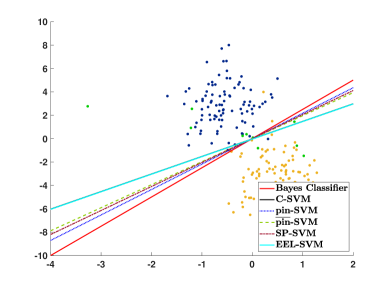
(b) Student’s $t$ distribution with 5 degrees of freedom

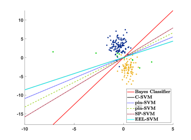
(c) Student’s $t$ distribution with 1 degree of freedom

Figure 1: Classification boundaries for five SVM classifiers if DU is induced by (a) Normal distribution, (b) Student’s $t$ distribution with 5 degrees of freedom and (c) Student’s $t$ distribution with 1 degree of freedom.

The scatter plots in Figure 1 explain the contamination mechanism, though these pictorial representations may be misleading due to the sampling error, since Figure 1 relies on a single random sample. Therefore, we repeat the same exercise $100$ times in order to properly compare the classifiers in Tables 2 and 3. Moreover, for each sample, we conduct $10$-fold cross-validation to tune the additional parameters, and we then compute the linear decision rule. The performance is measured via the distance (4.2), and the summary of this analysis is provided in Table 2 for samples of size $N\in\{100,200\}$ and a contamination ratio $r\in\{0.05,0.10\}$. Note that the tuning parameters are calibrated as in Section 4.1.1, except EEL-SVM, where the parameter space is enlarged (due to data contamination) as follows:

$$\mathcal{A}_{EEL}:=\left\{\begin{array}[]{cc}\{0,0.01,\dots,0.05\}&\text{if }r=0.05;\\ \{0,0.01,\dots,0.10\}&\text{if }r=0.10.\end{array}\right.$$

EEL-SVM requires a larger parameter space when DU is more pronounced, i.e. $r=0.10$, but even in this extreme case the cardinality of $\mathcal{A}_{EEL}$ is not larger than the cardinality of any other parameter space. That is, we do not favor EEL-SVM in the implementation phase.

	Normal distribution
	$r=0.05$		$r=0.10$
	$N=100$	$N=200$	$N=100$	$N=200$
C-SVM	0.8397	0.6623	1.1455	0.8675
$pin$-SVM	0.0704	0.1880	0.2955	0.2996
$\overline{pin}$-SVM	0.3073	0.3984	0.7334	0.4611
SP-SVM	0.2305	0.2994	0.5938	0.2813
EEL-SVM	0.8431	0.6788	1.1682	0.8785
	Student’s $t$ distribution (5 degrees of freedom)
	$r=0.05$		$r=0.10$
	$N=100$	$N=200$	$N=100$	$N=200$
C-SVM	1.1520	0.6795	1.4983	0.9863
$pin$-SVM	0.2966	0.1710	0.6861	0.3322
$\overline{pin}$-SVM	0.5929	0.3410	0.9491	0.6492
SP-SVM	0.7405	0.3754	0.8801	0.4539
EEL-SVM	1.1560	0.6895	1.5077	1.0025
	Student’s $t$ distribution (1 degree of freedom)
	$r=0.05$		$r=0.10$
	$N=100$	$N=200$	$N=100$	$N=200$
C-SVM	1.8189	2.0358	2.6941	3.2549
$pin$-SVM	1.1983	1.6466	2.0853	2.1472
$\overline{pin}$-SVM	1.4458	1.3479	1.9612	2.4647
SP-SVM	1.2384	1.2675	1.8261	1.8463
EEL-SVM	1.8558	2.0280	2.6788	3.2757

Table 2: Distance (4.2) between various SVM classifiers and Bayes classifier for contaminated synthetic data. The lowest distance for each row is in bold.

Table 2 shows that the performance of any classifier deteriorates when the level of DU increases; moreover, the distance from the Bayes classifier increases with the contamination ratio $r$. The overall performances of SP-SVM and $pin$-SVM are superior to all other three competitors, whereas $\overline{pin}$-SVM appears to be competitive in just a few cases and C-SVM and EEL-SVM have a similar low performance. SP-SVM is by far the most robust classifier when DU is more pronounced, which has been observed in Figure 1 (c) but for a single sample.

	Normal distribution
	$r=0.05$		$r=0.10$
	$N=100$	$N=200$	$N=100$	$N=200$
$pin$-SVM	15.5138	33.9715	19.2942	39.8558
$\overline{pin}$-SVM	30.1658	22.9012	36.6373	32.7994
SP-SVM	7.6634	15.3068	9.2248	16.7844
EEL-SVM	6.6263	14.0950	8.6631	16.1476
	Student’s $t$ distribution (5 degrees of freedom)
	$r=0.05$		$r=0.10$
	$N=100$	$N=200$	$N=100$	$N=200$
$pin$-SVM	12.6893	41.3835	17.0174	44.2939
$\overline{pin}$-SVM	42.1007	26.7222	61.5340	27.6636
SP-SVM	6.1618	19.6716	7.7810	17.8432
EEL-SVM	5.6473	17.2680	7.7076	17.6688
	Student’s $t$ distribution (1 degree of freedom)
	$r=0.05$		$r=0.10$
	$N=100$	$N=200$	$N=100$	$N=200$
$pin$-SVM	11.4355	34.5926	15.0441	41.0832
$\overline{pin}$-SVM	25.4353	42.4561	45.9922	62.0633
SP-SVM	5.9118	15.5805	7.3598	17.8881
EEL-SVM	5.1893	14.5320	7.1204	16.3805

Table 3: Computational time ratios of SVM classifiers compared to C-SVM classifier for contaminated synthetic data. The lowest computational time ratio for each row is in bold.

We conclude our comparison by looking into the computational time ratios (with C-SVM being the baseline reference) that are reported in Table 3. In particular, this provides the computational times after tuning each model, i.e. the training computational time, which is a standard and fair reporting when one would expect high computational times when tuning more model hyper-parameters. EEL-SVM requires the lowest computational effort, though it is very close to SP-SVM, while $pin$-SVM is consistently slower and $\overline{pin}$-SVM is by far the method with the largest computational time. These observations are not surprising because $\overline{pin}$-SVM relies on a non-convex (DCA) algorithm that has scalability issues; on the contrary, $pin$-SVM, SP-SVM and EEL-SVM are solved via convex LCQP of the same dimension, though EEL-SVM and $pin$-SVM are, respectively, the most and least sparse.

4.2 Real Data Analysis

We now compare the classification accuracy for some real-life data and rank all six SVM classifiers, including Ramp-KSVCR. Ten well-known real-world datasets are chosen in this section, which can be retrieved from the UCI depository and LIBSVM depository; a summary is given in Table 4. It should be noted that all datasets have features rescaled to $[-1,1]$. Moreover, the analysis is carried out over the original and contaminated data. DU is introduced via the MATLAB R2019a function awgn with different Signal Noise Ratios (SNR); perturbations are separately introduced $10$ times for each dataset before training, and the average classification accuracy is reported so that the sampling error is alleviated.

	Data	Number of	Training	Testing
		features	sample size	sample size
(I)	Fourclass	2	580	282
(II)	Diabetes	8	520	248
(III)	Breast cancer	10	460	223
(IV)	Australian	14	470	220
(V)	Statlog	13	180	90
(VI)	Customer	7	300	140
(VII)	Trial	17	520	252
(VIII)	Banknote	4	920	452
(IX)	A3a	123	3,185	29,376
(X)	Mushroom	112	2,000	6,124

Table 4: Summary of the ten UCI datasets.

The data are randomly partitioned into the training and testing sets, as described in Table 4. All SVM methods rely on the Radial Basis Function (RBF) kernel chosen to overcome the lack of linearity in the data. As before, SP-SVM methodology assumes that the feature with the largest standard deviation is the one mostly affected by DU. All hyper-parameters are tuned via a $10$-fold cross-validation; the kernel parameter $\gamma$ and penalty parameter $C$ are tuned by allowing $\gamma,C\in\big{\{}2^{-9},2^{-8},\dots,2^{8},2^{9}\big{\}}$ for C-SVM, while $C\in\big{\{}2^{-5},2^{-3},2^{-1},2^{0},2^{1},2^{3},2^{5}\big{\}}$ and $\gamma\in\big{\{}2^{-7},2^{-5},2^{-3},2^{-1},2^{0},2^{1}\big{\}}$ are allowed for all other classifiers. Note that C-SVM has fewer parameters than other classifiers, and thus, $(\gamma,C)$ are allowed more values in the tuning process, so that all classifiers are treated as equally as possible. Note that Ramp-KSVCR has two penalty parameters $C_{1},C_{2}$, an insensitivity parameter $\epsilon$ and two additional model parameters $s$ and $t$; the penalty parameters satisfy $C_{1}=C_{2}$, as in the original paper. The other parameters are tuned as follows:

• SP-SVM: $\alpha\in\mathcal{A}_{SP}=\{0.50,0.51,\dots,0.56,0.58,0.60\}$;

• EEL-SVM: $\alpha\in\mathcal{A}_{EEL}=\{0,0.05,0.10,\dots,0.3\}$;

• $pin$-SVM: $\tau\in\mathcal{T}_{pin}=\{0.1,0.2,\dots,0.8,1\}$;

• $\overline{pin}$-SVM$:s\in\{0.01,0.1,0.3,0.5,0.7,1\}$ and $\tau=0.5$;

• Ramp-KSVCR: $\epsilon\in\{0.1,0.2,0.3\},t\in\{1,3,5\},s=-1$.

A final note is that a computational budget of around $370$ parameter combinations is imposed on all cases, except EEL-SVM where $294$ combinations are considered.

Data	SNR	C-	$pin$-	$\overline{pin}$-	SP-	EEL-	Ramp-
		SVM	SVM	SVM	SVM	SVM	KSVCR
(I)	NA	99.29%	99.29%	99.65%	99.65%	99.65%	92.20%
	10	99.65%	99.65%	99.65%	99.61%	99.75%	91.95%
	5	99.65%	99.65%	99.65%	99.54%	99.72%	91.67%
	1	99.54%	99.61%	99.61%	99.50%	99.65%	91.84%
(II)	NA	77.02%	79.84%	79.84%	80.24%	78.63%	80.24%
	10	76.98%	76.49%	78.10%	79.64%	77.26%	77.10%
	5	76.69%	76.57%	77.54%	78.02%	76.45%	79.48%
	1	76.49%	77.70%	76.90%	77.66%	74.96%	79.44%
(III)	NA	93.72%	93.27%	94.17%	94.62%	93.72%	95.96%
	10	93.90%	94.75%	93.86%	93.32%	94.44%	95.29%
	5	93.86%	94.57%	94.17%	94.13%	94.08%	94.80%
	1	93.81%	93.86%	93.86%	93.86%	94.04%	95.11%
(IV)	NA	88.64%	88.18%	89.55%	88.18%	89.09%	89.55%
	10	85.82%	85.23%	85.77%	85.45%	85.32%	83.82%
	5	80.68%	80.50%	82.41%	80.59%	78.45%	77.73%
	1	76.59%	75.86%	77.86%	76.14%	76.23%	75.77%
(V)	NA	82.22%	82.22%	82.22%	83.33%	78.89%	80.00%
	10	80.22%	80.56%	77.56%	80.22%	82.44%	81.00%
	5	80.00%	79.33%	79.89%	79.33%	81.33%	77.00%
	1	78.67%	78.22%	80.00%	78.44%	76.89%	80.22%
(VI)	NA	92.14%	91.43%	90.71%	92.14%	92.86%	91.89%
	10	92.86%	92.50%	92.50%	92.71%	93.21%	89.93%
	5	92.93%	92.86%	91.43%	93.07%	93.07%	91.36%
	1	92.57%	92.93%	91.57%	92.57%	92.86%	90.79%
(VII)	NA	100.00%	100.00%	100.00%	100.00%	100.00%	100.00%
	10	99.56%	99.80%	99.33%	99.76%	99.60%	99.48%
	5	94.72%	94.60%	94.44%	94.84%	94.52%	93.97%
	1	88.13%	88.13%	85.99%	88.29%	88.21%	86.98%
(VIII)	NA	100.00%	100.00%	100.00%	100.00%	100.00%	100.00%
	10	99.73%	99.71%	99.80%	99.76%	99.89%	99.85%
	5	99.38%	99.18%	99.05%	99.25%	99.36%	99.05%
	1	97.94%	97.92%	97.61%	97.94%	97.83%	96.75%
(IX)	NA	82.81%	83.20%	83.36%	83.67%	81.71%	84.04%
	10	80.50%	81.05%	80.57%	81.12%	81.15%	81.13%
	5	78.57%	78.56%	77.94%	78.35%	78.26%	78.00%
	1	76.34%	76.74%	75.94%	76.01%	76.02%	76.25%
(X)	NA	99.87%	99.87%	99.87%	99.87%	99.87%	99.87%
	10	98.37%	98.84%	99.38%	98.31%	98.29%	99.03%
	5	93.02%	93.79%	94.72%	93.05%	92.92%	93.77%
	1	85.36%	85.63%	85.82%	85.46%	85.47%	85.55%
Average rank		3.25	3.18	3.18	2.93	3.05	3.53

Table 5: Classification accuracy (in $\%$) of all SVM classifiers across all datasets. The highest accuracies for each row are in bold. Each row signifies the original data (reported as “NA”, i.e. no contamination) or their contaminated variants (with SNR values of $\{1,5,10\}$).

Table 5 summarizes the classification performance for all ten datasets for the original (non-contaminated) data and their contaminated variants with various SNR values, where smaller SNR value means higher degree of data contamination. EEL-SVM achieves the best performance in 14 out of 40 scenarios investigated, which is followed by Ramp-KSVCR that performs best in 13 out of 40 scenarios; the other classifiers are ranked as follows: SP-SVM (11/40), $\overline{pin}$-SVM (10/40), C-SVM (7/40) and $pin$-SVM (6/40). We also calculate the average ranks for each classifier by looking at each row of Table 5 and rank each entry from 1 to 6 from lowest to highest accuracy; SP-SVM and EEL-SVM yield the best average ranks among all classifiers and SP-SVM outperforms its competitors via this criterion.

In summary, SP-SVM and EEL-SVM exhibit competitive advantage over their competitors, with EEL-SVM being more sparse, though SP-SVM seems to be performing slightly better.

4.3 Interpretable Classifiers

The performance of SVM classifiers for real-life data has been analyzed in Section 4.2 without interpreting the decision rules so that the presence of DU is better understood and the fairness of the decision is assessed. We achieve that now by providing a granular analysis for classification of the US mortgage lending data that are downloaded from the Home Mortgage Disclosure Act (HMDA) website (https://ffiec.cfpb.gov). Specifically, we collected the 2020 data for two states, namely, Maine (ME) and Vermont (VT), with a focus on subordinated lien mortgages.

Subordinate-lien (‘piggyback’) loans are taken out at the same time as first-lien mortgages on the same property by borrowers, mainly to avoid paying mortgage insurance on the first-lien mortgage (due to the extra down payment). Eriksen et al. (2013) find evidence that borrowers with subordinate loans have an increased by 62.7% chance to default each month on primary loan. Such borrowers may sequentially default on each loan since subordinate lenders will not pursue foreclosure if the borrowers have insufficient equity until at least housing markets start to recover. As noted by Soyer and Xu (2010), due to major costs from default for all involved parties, including mortgage lenders and mortgagors, the modelling, assessment, and management of mortgage default risk (e.g., Bhattacharya et al., 2019) is a major concern for financial institutions and policy makers.

Subordinate-lien loans are high-risk mortgages and we aim to classify the instances as ‘loan originated’ ($Y=+1$) or ‘application denied’ ($Y=-1$) using the available features. The HMDA data have numerous features and the following representative ones are chosen: F1) loan amount, F2) loan to value ratio (F1 divided by the ‘property_value’), F3) percentage of minority population to total population for tract, F4) percentage of tract median family income compared to MSA (metropolitan statistical area) median family income. Two categorical features are also considered, namely, F5) derived sex and F6) age.

All categorical features are pre-processed via the standard one-hot encoding procedure and all features are rescaled to $[-1,1]$ before training. A random sampling is performed to extract the training and testing sets, so the training set is twice as large as the testing set. The hyper-parameter tuning of the three methods (C-SVM, SP-SVM, EEL-SVM) is performed via $10$-fold cross-validation using the hyper-parameter spaces in Section 4.2. SP-SVM identifies F1 (loan amount) as the feature affected by DU, which has the largest standard deviation at the same time. This is not surprising since the loan amount has a massive impact on the mortgage lending decision and this feature is heavily influenced by all other features. Table 6 reports the details of the training-testing splitting and the out-of-sample accuracy of the three SVM methods.

Dataset	Total	Testing	C-SVM	SP-SVM	EEL-SVM
	sample size	sample size
ME	4,226	1,396	70.77%	70.77%	70.13%
VT	1,948	648	90.74%	91.67%	90.89%

Table 6: Summary of the HMDA datasets and their accuracy levels. The highest accuracy for each row is in bold.

We observe that SP-SVM performs best in terms of accuracy, with C-SVM and EEL-SVM relatively close. The next step is to interpret the classification rule and explain the DU effect, but also evaluate the effect of an automatized mortgage lending decision. The latter is measured by looking into unfavorable decisions where the loan is denied, i.e. $Y=-1$.

The Equal Credit Opportunity Act (ECOA) prohibits a creditor from discriminating against any borrower on the basis of age, marital status, race, religion, or sex, known as protected characteristics; such a regulatory requirement is imposed not only in the US, but also similar ones are in place in the EU, UK and elsewhere. Under ECOA, regulatory agencies assess the lending decision fairness of lending institutions by comparing the unfavorable decision ($Y=-1$) across different groups with given protected characteristics. Our next analysis focuses on checking whether an automatized lending decision could lead to unintentional discrimination, known as disparate impact. First, we look at the entry data and provide evidence on whether or not the loan amount is massively different across the applicants’ gender at birth, income and racial structure in their postal code, which would explain if DU is present or not. Second, we evaluate the fairness of the lending decision obtained via SVM classification and argue which SVM-based decision is more compliant with such non-discrimination regulation (with respect to the sex attribute).

		Training data			Testing data
		MvsF	MvsJ	FvsJ	MvsF	MvsJ	FvsJ
ME	$Y\in\{-1,1\}$	0.0853	0.0477	0.1330	0.0969	0.1248	0.2096
	$Y=-1$	0.0540	0.0727	0.1215	0.1203	0.1122	0.2313
	$Y=1$	0.1091	0.0381	0.1472	0.0889	0.1266	0.1986
VT	$Y\in\{-1,1\}$	0.0923	0.1009	0.1841	0.1355	0.1399	0.2000
	$Y=-1$	0.0866	0.0449	0.1208	0.3095	0.1429	0.1667
	$Y=1$	0.1258	0.1579	0.2515	0.1235	0.1575	0.2108

Table 7: Kolmogorov–Smirnov distances in the loan amount distribution of males versus females (MvsF), males versus joint (MvsJ) and females versus joint (FvsJ). The largest distances for each row corresponding to training and testing data are in bold.

Table 7 reports the Kolmogorov–Smirnov distances for loan amount samples of applicants based on gender characteristics. There is overwhelming evidence that joint loan applications and female applicants have very different loan amount distributions in both training and testing data, though VT data exhibit the largest distance when comparing male and female applicants with a favorable mortgage lending decision. This could be explained by socio-economic disparities between males and females, though DU plays a major role in this instance. Gender information in the HMDA data is expected to have a self-selection bias, since applicants at risk are quite unlikely to report gender information as they believe that the lending decision would be influenced by that. Consequently, we removed a significant portion of the data, i.e. examples for which the gender information is unknown, which is clear evidence of self-selection bias in our entry data.

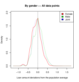
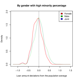
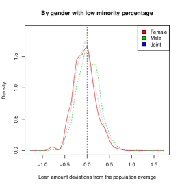
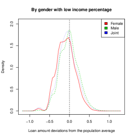
Figure 2: ME loan amount deviations from the population mean based on full data and sub-populations with low/high minority and low/high income percentages.

Figures 2 and 3 show the kernel densities of the deviation of the log-transformed loan amount from the population mean. In particular, we plot such deviations for the entire dataset, but also for sub-populations with low/high minority and income percentage. Low/high minority percentage means that the mortgage applicant is in an area of lower/higher minority than the population median. Moreover, low/high income percentage means that the mortgage applicant household income is lower/higher than the household income in her/his MSA. ME data from Figures 2 do not show any evidence of DU with respect to the loan amount, which explains the results in Table 6 where SP-SVM and EEL-SVM did not improve the non-robust counterpart. VT data show a very different scenario in Figure 3, where the loan amount deviations have a bimodal distribution. In addition, within the low minority sub-population, female applicants exhibit significantly lower loan amounts than all other applicants; the same pattern is observed in the low income sub-population. Therefore, the DU in the VT data is evident, and confirms the findings in Table 7, but also those in Table 6 where SP-SVM and EEL-SVM did improve the non-robust C-SVM.

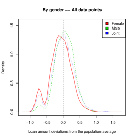
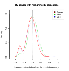
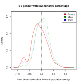
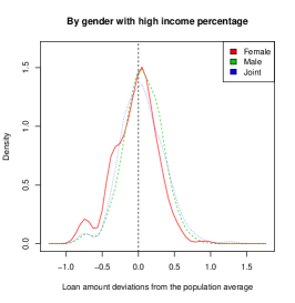
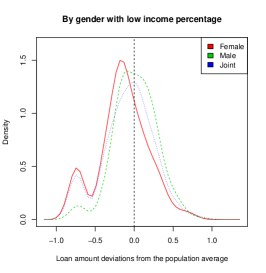
Figure 3: VT loan amount deviations from the population mean based on full data and sub-populations with low/high minority and low/high income percentages.

We have concluded the first part of our qualitative analysis, where we have explained the DU, and we now evaluate how much compliant the automatized mortgage lending process would be for the VT data; we do not report the ME results due to lack of DU. Fairness compliance requires the lending decision – especially the unfavorable decisions ($Y=-1$) – to be independent of the applicant’s gender at birth information, i.e.

$$\Pr(Y=-1)=\Pr(Y=-1|S=l)\quad\text{for all}\quad l\in\mathcal{S}:=\{Female,Male,Joint\}.$$ (4.3)

	C-SVM	SP-SVM	EEL-SVM	True
$\Pr(Y=-1)$	2.3148%	1.0802%	5.5556%	7.8704%
$\Pr(Y=-1|\text{Female})$	3.9683%	1.5873%	6.3492%	9.5238%
$\Pr(Y=-1|\text{Male})$	7.8125%	3.9063%	10.1563%	16.4062%
$\Pr(Y=-1|\text{Joint})$	0.0000%	0.0000%	3.8071%	4.5685%
$\Pr(Y=-1|\text{Low\ Income})$	2.9316%	0.9772%	5.5375%	8.0495%
$\Pr(Y=-1|\text{High\ Income})$	1.7595%	1.1730%	5.5718%	7.6923%
$\Pr(Y=-1|\text{Low\ Minority})$	1.8576%	0.9290%	5.5728%	9.7720%
$\Pr(Y=-1|\text{High\ Minority})$	2.7692%	1.2308%	5.5385%	6.1584%
$CDD$	-25.5944%	-25.2601%	-8.3263%	-11.3792%

Table 8: Probability of a denied loan for the three classification methods. The closest value (per row) to the ‘true’ probability is in bold.

Table 8 tells us that the desirable lack of disparity in (4.3) is achieved best by EEL-SVM. In addition, EEL-SVM estimates the unfavorable decisions very similarly to the ‘true’ decisions and this could be seen by inspecting the probabilities that appear in bold.

One popular fairness metric is the Conditional Demographic Disparity (CDD), which is discussed in Wachter et al. (2021), where the data are assumed to be part of multiple strata. The CDD formulation for our data (with three strata, i.e. Female, Male and Joint) is defined as

$$CDD=\sum_{l\in\mathcal{S}}\Pr(S=l)\times DD_{l},$$

where $DD_{l}$ is the demographic disparity within the $l^{th}$ stratum, i.e.

$$DD_{l}=\Pr(S=l\mid Y=-1)-\Pr(S=l\mid Y=1)\quad\text{for all}\quad l\in\mathcal{S}.$$

CDD could capture and explain peculiar data behavior similar to Simpson’s paradox where the same trend is observed in each stratum, but the opposite trend is observed in the whole dataset. Amazon SageMaker, a cloud machine-learning platform developed by Amazon, has included CDD in their practice to enhance model explainability and bias detection; for details, see the Amazon SageMaker Developer Guide.

Table 8 shows that EEL-SVM has superior performance to C-SVM and SP-SVM when looking at the overall CDD fairness performance. In fact, EEL-SVM exhibits fairer post-training decisions than the pre-training fairness measured on the ‘true’ mortgage lending decisions observed in the testing data. In summary, the unanimous conclusion is that EEL-SVM shows the fairest and most robust mortgage lending automatized decision.

5 Conclusions and Future Work

This paper addresses the problem of binary classification under DU. Two robust SVM-like classification algorithms are developed, namely, SP-SVM and EEL-SVM, and there is sufficient empirical evidence to conclude that the new classifiers are very competitive when compared to other well-known SVM robust competitors. One could argue that SP-SVM shows slightly better classification performance than EEL-SVM and various alternatives, but there is an irrefutable evidence about the computational time, with both SP-SVM and EEL-SVM exhibiting significant competition advantage over all other choices.

Future research would be required to extend our probabilistic arguments to multi-class classification problems, which is a non-trivial problem. We also plan to adapt our SP-SVM and EEL-SVM to imbalanced data, which is another research direction for future investigation.

EC A.1 Appendix

A.1.1 Proof of Theorem 1

It is sufficient to show that (2.4) holds when $p>q$ and $p<q$, where

$$p:=\Pr\big{(}Y=1|\textbf{x}\big{)}\quad\mbox{and}\quad q:=\Pr\big{(}Y=-1|\textbf{x}\big{)}.$$

The latter is equivalent to

$$\operatorname*{arg\,min}_{z\in\mathbb{R}}\mathbf{E}_{\mathcal{Y}|\textbf{x}}L\Big{(}1\!-\!Yz\Big{)}=\operatorname*{arg\,min}_{z\in\mathbb{R}}pL(1\!-\!z)+qL(1\!+\!z)=\left\{\begin{array}[]{rll}1,&\text{if}&p>q,\\ -1,&\text{if}&p<q.\end{array}\right.$$ (A.3)

Note that $L(1\pm\cdot)$ are compositions of the convex function $L$ with affine mappings, and therefore, the objective function of (A.3) is convex. Moreover, the left and right derivatives of $L$ exist as the loss function is convex.

Assume first that $p>q$. The left and right derivatives at $1$ of the objective function in (A.3) are $-pL^{\prime}(0^{+})+qL^{\prime}(2^{-})$ and $-pL^{\prime}(0^{-})+qL^{\prime}(2^{+})$, respectively. Clearly,

$$-pL^{\prime}(0^{+})+qL^{\prime}(2^{-})=L^{\prime}(0^{+})(q-p)\leq 0$$

is true as $L$ is linear on $(0,2+\epsilon)$ for some $\epsilon>0$. Further,

$$\quad-pL^{\prime}(0^{-})+qL^{\prime}(2^{+})\geq 0$$

also holds due to the fact that $L^{\prime}(0^{-})\leq 0\leq L^{\prime}(2^{+})$, which is a consequence of the convexity of $L$ that attains its global minimum at $0$. Thus, the global minimum of (A.3) is attained at $1$ whenever $p>q$.

Assume now that $p<q$. Similarly, the left and right derivatives at $-1$ of the objective function in (A.3) are $-pL^{\prime}(2^{+})+qL^{\prime}(0^{-})$ and $-pL^{\prime}(2^{-})+qL^{\prime}(0^{+})$, respectively. Clearly, $-pL^{\prime}(2^{+})+qL^{\prime}(0^{-})\leq 0$ holds as $L^{\prime}(0^{-})\leq 0\leq L^{\prime}(2^{+})$ and $L$ is convex attaining its global minimum at $0$. Further, $-pL^{\prime}(2^{-})+qL^{\prime}(0^{+})=L^{\prime}(0^{+})(q-p)\geq 0$ is true as $L$ is linear on $(0,2+\epsilon)$ for some $\epsilon>0$. Thus, the global minimum of (A.3) is attained at $-1$ whenever $p<q$. This completes the proof.

A.1.2 Explicit Solution for (3.4)

Let $\phi_{j}\big{(}\mathbf{x}_{i}\big{)}$ be the $j^{th}$ element of $\phi\big{(}\mathbf{x}_{i}\big{)}$. Denote by $\phi_{1}\big{(}\mathbf{x}_{i}\big{)}$ and $\phi_{2}\big{(}\mathbf{x}_{i}\big{)}$ two vectors with their $j^{th}$ elements given by $\phi_{1j}\big{(}\mathbf{x}_{i}\big{)}=\phi_{j}\big{(}\mathbf{x}_{i}\big{)}-a_{ik}I_{j=k}$ and $\phi_{2j}\big{(}\mathbf{x}_{i}\big{)}=\phi_{j}\big{(}\mathbf{x}_{i}\big{)}+a_{ik}I_{j=k}$ for all $1\leq i\leq N$ and $1\leq j\leq d$, where $I_{A}$ is the indicator of set $A$ that takes the values $1$ or $0$ if $A$ is true or false, respectively. Thus, (3.4) could be written as

$$\begin{array}[]{lllrl}&\underset{\mathbf{w},b,\bm{\xi}}{\text{min}}&\frac{1}{2}\mathbf{w}^{T}\mathbf{w}+C\displaystyle\sum_{i=1}^{N}\xi_{i}&&\\ &\;\;\text{s.t.}&y_{i}\Big{(}\mathbf{w}^{T}\phi\big{(}\mathbf{x}_{i}\big{)}+b\Big{)}\geq 1-\xi_{i},&\xi_{i}\geq 0,&1\leq i\leq N,\\ &&y_{i}\big{(}\mathbf{w}^{T}\phi_{k}(\mathbf{x}_{i})+b\big{)}\geq 1-\xi_{i},&k\in\{1,2\},&1\leq i\leq N.\end{array}$$ (A.7)

It should be noted that the above is a convex quadratic optimization problem that has only affine constraints, and thus, strong duality holds. The dual of (A.7) is given by

$$\begin{array}[]{llll}&\underset{\bm{\alpha},\bm{\beta},\bm{\gamma},\bm{\delta}\geq\textbf{0}}{\text{max}}&-\frac{1}{2}\big{[}\bm{\alpha}\;\bm{\beta}\;\bm{\gamma}\big{]}^{T}\;\textbf{T}\;\big{[}\bm{\alpha}\;\bm{\beta}\;\bm{\gamma}\big{]}+\textbf{1}^{T}\bm{\alpha}+\textbf{1}^{T}\bm{\beta}+\textbf{1}^{T}\bm{\gamma}&\\ &\;\;\;\;\;\text{s.t.}&\bm{\alpha}+\bm{\beta}+\bm{\gamma}+\bm{\delta}=C\textbf{1},&\\ &&\textbf{y}^{T}\bm{\alpha}+\textbf{y}^{T}\bm{\beta}+\textbf{y}^{T}\bm{\gamma}=0,&\end{array}$$ (A.11)

where the block matrix T is given by

$$\textbf{T}=\left[\begin{array}[]{c|c|c}\textbf{T}^{\phi,\phi}&\textbf{T}^{\phi,\phi_{1}}&\textbf{T}^{\phi,\phi_{2}}\\ \hline\cr\textbf{T}^{\phi_{1},\phi}&\textbf{T}^{\phi_{1},\phi_{1}}&\textbf{T}^{\phi_{1},\phi_{2}}\\ \hline\cr\textbf{T}^{\phi_{2},\phi}&\textbf{T}^{\phi_{2},\phi_{1}}&\textbf{T}^{\phi_{2},\phi_{2}}\end{array}\right]$$

with $\textbf{T}^{\varphi_{1},\varphi_{2}}$ being an $N\times N$ matrix with the $(i,j)^{th}$ entry given by $y_{i}\varphi_{1}^{T}(\mathbf{x}_{i})\varphi_{2}(\mathbf{x}_{i})y_{j}$ for all $\varphi_{1},\varphi_{2}\in\{\phi,\phi_{1},\phi_{2}\}$ and $1\leq i,j\leq N$. Clearly, (A.11) is equivalent to solving

$$\begin{array}[]{llll}&\underset{\bm{\alpha},\bm{\beta},\bm{\gamma}\geq\textbf{0}}{\text{min}}&\frac{1}{2}\big{[}\bm{\alpha}\;\bm{\beta}\;\bm{\gamma}\big{]}^{T}\;\textbf{T}\;\big{[}\bm{\alpha}\;\bm{\beta}\;\bm{\gamma}\big{]}-\textbf{1}^{T}\bm{\alpha}-\textbf{1}^{T}\bm{\beta}-\textbf{1}^{T}\bm{\gamma}&\\ &\;\;\;\;\text{s.t.}&\bm{\alpha}+\bm{\beta}+\bm{\gamma}\leq C\textbf{1},&\\ &&\textbf{y}^{T}\bm{\alpha}+\textbf{y}^{T}\bm{\beta}+\textbf{y}^{T}\bm{\gamma}=0.&\end{array}$$ (A.16)

Let $(\bm{\alpha}^{*},\bm{\beta}^{*},\bm{\gamma}^{*})$ be an optimal solution of (A.16), which now helps with finding an optimal solution of (3.4), which, in turn, gives us the classification rule identified by $\textbf{w}^{*}$ and $b^{*}$. Clearly,

$$\textbf{w}^{*}:=\sum_{i=1}^{N}\big{(}\alpha_{i}^{*}y_{i}\phi(\mathbf{x}_{i})+\beta_{i}^{*}y_{i}\phi_{1}(\mathbf{x}_{i})+\gamma_{i}^{*}y_{i}\phi_{2}(\mathbf{x}_{i})\big{)}.$$

The choice of $b^{*}$ is possible by considering the complementary slackness conditions of (A.7). A sensible estimate of $b^{*}$ is $\widehat{\hskip 1.0ptb^{*}}:=\widehat{\hskip 1.0ptb^{+}_{l}}/|\mathcal{S}_{l}|$, where $|\mathcal{S}_{l}|$ represents the cardinality of $\mathcal{S}_{l}$ which is the set with the largest cardinality among

$$\mathcal{S}_{k}:=\big{\{}1\leq i\leq N:\;\theta_{ik}^{*}(C-\alpha_{i}-\beta_{i}-\gamma_{i})>0\big{\}},$$

where $\theta_{i0}^{*}=\alpha_{i}^{*}$, $\theta_{i1}^{*}=\beta_{i}^{*}$ and $\theta_{i2}^{*}=\gamma_{i}^{*}$ for all $1\leq i\leq N$, and

$$\widehat{\hskip 1.0ptb^{+}_{l}}:=\!\sum_{j\in\mathcal{S}_{l}}y_{j}-\!\sum_{j\in\mathcal{S}_{l}}\sum_{i=1}^{N}\big{(}\alpha^{*}_{i}y_{i}\phi^{T}(\mathbf{x}_{i})\phi(\mathbf{x}_{j})+\beta^{*}_{i}y_{i}\phi_{1}^{T}(\mathbf{x}_{i})\phi(\mathbf{x}_{j})+\gamma^{*}_{i}y_{i}\phi_{2}^{T}(\mathbf{x}_{i})\phi(\mathbf{x}_{j})\big{)}.$$

A.1.3 Explicit Solution for (3.7)

The derivations in this section are quite similar to those in Appendix A.1.2, and thus, we provide only the main steps. Note that the convex quadratic instance (3.7) has only affine constraints, and therefore, the strong duality holds. One may show that the dual of (3.7) is equivalent to solving

$$\begin{array}[]{llll}&\underset{\bm{\alpha},\bm{\beta},\bm{\gamma}\geq\textbf{0}}{\text{min}}&\frac{1}{2}\bm{\alpha}\;\textbf{T}^{\phi,\phi}\;\bm{\alpha}-\textbf{1}^{T}\bm{\alpha}&\\ &\;\;\text{s.t.}&\bm{\alpha}+\bm{\beta}+\bm{\gamma}=D_{1}\textbf{1},\\ &&\textbf{y}^{T}\bm{\alpha}=0,\\ &&\textbf{1}^{T}\bm{\alpha}+\textbf{1}^{T}\bm{\beta}=D,\end{array}$$ (A.21)

where $\textbf{T}^{\phi,\phi}$ is as defined in Appendix A.1.2 and $D_{1}:=D/N(1-\alpha)$. Once again, (3.7) and (A.21) are equivalent due to strong duality arguments.

Let $(\bm{\alpha}^{*},\bm{\beta}^{*},\bm{\gamma}^{*})$ be an optimal solution of (A.21). Then, (3.7) is solved with

$$\textbf{w}^{*}=\sum_{i=1}^{N}\alpha_{i}^{*}y_{i}\phi(\mathbf{x}_{i}).$$

Finally, the bias term $b^{*}$ could be estimated as follows

$$\big{(}\widehat{\hskip 1.0ptb^{*}},\widehat{\hskip 1.0ptz^{*}}\big{)}:=\left\{\begin{array}[]{cc}\big{(}\widehat{\hskip 1.0ptb^{*1}},0\big{)}&\text{if}\quad|\mathcal{S}_{4}|\leq|\mathcal{S}_{3}|,\\ \big{(}\widehat{\hskip 1.0ptb^{*2}},0\big{)}&\text{if}\quad|\mathcal{S}_{4}|>|\mathcal{S}_{3}|,\end{array}\right.$$

where

$$\widehat{\hskip 1.0ptb^{*1}}\!=\!\frac{\widehat{\hskip 1.0ptb^{+}_{3}}}{|\mathcal{S}_{3}|},\;\;\widehat{\hskip 1.0ptb^{+}_{3}}\!=\!\sum_{j\in\mathcal{S}_{3}}y_{j}\!-\!\sum_{j\in\mathcal{S}_{3}}\sum_{i=1}^{N}\alpha^{*}_{i}y_{i}\phi^{T}(\mathbf{x}_{i})\phi(\mathbf{x}_{j}),$$

$$\widehat{\hskip 1.0ptb^{*2}}\!=\!\frac{\widehat{\hskip 1.0ptb^{+}_{4}}}{|\mathcal{S}_{4}|},\;\;\widehat{\hskip 1.0ptb^{+}_{4}}\!=\!\sum_{j\in\mathcal{S}_{4}}y_{j}\!-\!\sum_{j\in\mathcal{S}_{4}}\sum_{i=1}^{N}\alpha^{*}_{i}y_{i}\phi^{T}(\mathbf{x}_{i})\phi(\mathbf{x}_{j}),$$

and

$$\mathcal{S}_{3}:=\big{\{}1\leq i\leq N:\;\alpha_{i}^{*}\beta_{i}^{*}\gamma_{i}^{*}>0\big{\}}\quad\text{and}\quad\mathcal{S}_{4}:=\big{\{}1\leq i\leq N:\;\alpha_{i}^{*}\beta_{i}^{*}>0,\gamma_{i}^{*}=0\big{\}}.$$

References

- Asimit et al. (2017) Asimit, A. V., Bignozzi, V., Cheung, K. C., Hu, J. and Kim, E. S. (2017) Robust and Pareto optimality of insurance contracts. European Journal of Operational Research, 262, 720–732.
- Bamakan et al. (2017) Bamakan, S. M. H., Wang, H. and Shi, Y. (2017) Ramp loss K-support Vector Classification-Regression; a robust and sparse multi-class approach to the intrusion detection problem. Knowledge-Based Systems, 126, 113–126.
- Bartlett et al. (2006) Bartlett, P. L., Jordan, M. I. and McAuliffe, J. D. (2006) Convexity, classification, and risk bounds. Journal of the American Statistical Association, 101, 138–156.
- Ben-Tal et al. (2011) Ben-Tal, A., Bhadra, S., Bhattacharyya, C. and Nath, J. S. (2011) Chance constrained uncertain classification via robust optimization. Mathematical Programming, 127, 145–173.
- Bertsimas et al. (2018) Bertsimas, D., Dunn, J., Pawlowski, C. and Zhuo, Y. D. (2018) Robust classification. Journal on Optimization, 1, 2–34.
- Bhattacharya et al. (2019) Bhattacharya, A., Wilson, S. P. and Soyer, R. (2019) A Bayesian approach to modeling mortgage default and prepayment. European Journal of Operational Research, 274, 1112–1124.
- Bi and Zhang (2005) Bi, J. and Zhang, T. (2005) Support vector classification with input data uncertainty. In Advances in Neural Information Processing Systems, 161–168.
- Brooks (2011) Brooks, J. P. (2011) Support vector machines with the ramp loss and the hard margin loss. Operations research, 59, 467–479.
- Cortes and Vapnik (1995) Cortes, C. and Vapnik, V. N. (1995) Support-vector networks. Machine Learning, 20, 273–297.
- Eriksen et al. (2013) Eriksen, M. D., Kau, J. B. and Keenan, D. C. (2013) The impact of second loans on subprime mortgage defaults. Real Estate Economics, 41, 858–886.
- Fan et al. (2016) Fan, J., Liao, Y. and Liu, H. (2016) An overview of the estimation of large covariance and precision matrices. The Econometrics Journal, 19, C1–C32.
- Fang et al. (1990) Fang, K. T., Kotz, S. and Ng, K. W. (1990) Symmetric multivariate and related distributions. Chapman & Hall/CRC.
- Gambella et al. (2021) Gambella, C., Ghaddar, B. and Naoum-Sawaya, J. (2021) Optimization problems for machine learning: A survey. European Journal of Operational Research, 290, 807–828.
- Huang et al. (2012) Huang, G., Song, S., Wu, C. and You, K. (2012) Robust support vector regression for uncertain input and output data. IEEE Transactions on Neural Networks and Learning Systems, 23, 1690–1700.
- Huang et al. (2014) Huang, X., Shi, L. and Suykens, J. A. (2014) Support vector machine classifier with pinball loss. IEEE Transactions on Pattern Analysis and Machine Intelligence, 36, 984–997.
- Lanckriet et al. (2002) Lanckriet, G. R. G., El Ghaoui, L., Bhattacharyya, C. and Jordan, M. L. (2002) A robust minimax approach to classification. Journal of Machine Learning Research, 3, 555–582.
- Ledoit and Wolf (2020) Ledoit, O. and Wolf, M. (2020) The power of (non-) linear shrinking: A review and guide to covariance matrix estimation. Journal of Financial Econometrics.
- Lin (2002) Lin, Y. (2002) Support vector machines and the Bayes rule in classification. Data Mining and Knowledge Discovery, 6, 259–275.
- Lin (2004) Lin, Y. (2004) A note on margin-based loss functions in classification. Statistics & Probability Letters, 68, 73–82.
- Rockafellar and Uryasev (2000) Rockafellar, R. T. and Uryasev, S. (2000) Optimization of conditional value-at-risk. Journal of Risk, 2, 21–42.
- Shen et al. (2017) Shen, X., Niu, L., Qi, Z. and Tian, Y. (2017) Support vector machine classifier with truncated pinball loss. Pattern Recognition, 68, 199–210.
- Singh et al. (2014) Singh, A., Pokharel, R. and Principe, J. C. (2014) The C-loss function for pattern classification. Pattern Recognition, 47, 441–453.
- Soyer and Xu (2010) Soyer, R. and Xu, F. (2010) Assessment of mortgage default risk via Bayesian reliability models. Applied Stochastic Models in Business and Industry, 26, 308–330.
- Suykens and Vandewalle (1999) Suykens, J. A. K. and Vandewalle, J. (1999) Least squares support vector machine classifiers. Neural Processing Letters, 9, 293–300.
- Trafalis and Gilbert (2006) Trafalis, T. B. and Gilbert, R. C. (2006) Robust classification and regression using support vector machines. European Journal of Operational Research, 173, 893–909.
- Vapnik (2000) Vapnik, V. N. (2000) The nature of statistical learning theory. New York: Springer, 2 edn.
- Wachter et al. (2021) Wachter, S., Mittelstadt, B. and Russell, C. (2021) Why fairness cannot be automated: Bridging the gap between eu non-discrimination law and ai. Computer Law & Security Review, 41, 105567.
- Wang et al. (2018) Wang, X., Fan, N. and Pardalos, P. M. (2018) Robust chance-constrained support vector machines with second-order moment information. Annals of Operations Research, 263, 45–68.
- Wu and Liu (2007) Wu, Y. and Liu, Y. (2007) Robust truncated hinge loss support vector machines. Journal of the American Statistical Association, 102, 974–983.
- Wu and Liu (2013) Wu, Y. and Liu, Y. (2013) Adaptively weighted large margin classifiers. Journal of Computational and Graphical Statistics, 22, 416–432.
- Xu et al. (2017) Xu, G., Cao, Z., Hu, B.-G. and Principe, J. C. (2017) Robust support vector machines based on the rescaled hinge loss function. Pattern Recognition, 63, 139–148.
- Xu et al. (2009) Xu, H., Caramanis, C. and Mannor, S. (2009) Robustness and regularization of support vector machines. Journal of Machine Learning Research, 10, 1485–1510.
- Yang et al. (2007) Yang, X., Song, Q. and Wang, Y. (2007) A weighted support vector machine for data classification. International Journal of Pattern Recognition and Artificial Intelligence, 21, 961–976.
- Zhang (2004) Zhang, T. (2004) Statistical analysis of some multi-category large margin classification methods. Journal of Machine Learning Research, 5, 1225–1251.