Accelerated derivative-free spectral residual method for nonlinear systems of equations

Abstract

Spectral residual methods are powerful tools for solving nonlinear systems of equations without derivatives. In a recent paper, it was shown that an acceleration technique based on the Sequential Secant Method can greatly improve its efficiency and robustness. In the present work, an R implementation of the method is presented. Numerical experiments with a widely used test bed compares the presented approach with its plain (i.e. non-accelerated) version that makes part of the R package BB. Additional numerical experiments compare the proposed method with NITSOL, a state-of-the-art solver for nonlinear systems. The comparison shows that the acceleration process greatly improves the robustness of its counterpart included in the existent R package. As a by-product, an interface is provided between R and the consolidated CUTEst collection, which contains over a thousand nonlinear programming problems of all types and represents a standard for evaluating the performance of optimization methods.

Key words: nonlinear systems, derivative-free, sequential residual methods, sequential secant approach, acceleration, numerical experiments.

1 Introduction

Solving nonlinear systems of equations is an ubiquitous problem that appears in a wide range of applied fields such as Physics, Chemistry, Engineering, and Statistics, just to name a few. Moreover, many times, equations are computed using black-box codes and derivatives are not available. Thus, derivative-free solution methods are in order.

Given $F:\mathbb{R}^{n}\to\mathbb{R}^{n}$, we consider the problem of finding $x\in\mathbb{R}^{n}$ such that

$$F(x)=0,$$ (1)

without making use of derivatives. Observing that (1) is equivalent to $x=x-\sigma F(x)$, for any $\sigma>0$, Sequential Residual Methods (namely SANE and DF-SANE) based on the iteration $x^{k+1}=x^{k}-\sigma_{k}F(x^{k})$, where

$$\sigma_{k}=\frac{\|s^{k-1}\|^{2}}{(y^{k-1})^{T}s^{k-1}},\;\;\;\;s^{k-1}=x^{k}-x^{k-1},\;\;\mbox{ and }\;\;y^{k-1}=F(x^{k})-F(x^{k-1}),$$

were introduced in [14] and [13]. These methods were inspired by the Barzilai-Borwein step of minimization methods; see [2, 17, 18]. Although very popular, in part due to its simplicity, these methods may suffer from slow convergence. On the other hand, their simple and fast iterations made them an adequate choice to provide a global convergent framework to the Sequential Secant approach [1, 22]. This choice was explored in [3], where the Accelerated DF-SANE method was introduced. Numerical experiments in [3] shown that Accelerated DF-SANE compares favorably to the classical truncated Newton approach implemented in the package NITSOL [16], when applied to large-scale problems coming from the discretization of partial differential equations.

In the present work, an R [20] implementation of Accelerated DF-SANE is introduced. Numerical experiments in [3] are complemented with numerical experiments using the widely-used testing environment for optimization CUTEst [11]. Problems in the CUTEst collection are given in SIF (Standard Input Format; see [9, Chapters 2 and 7]) and a decoder named SifDec translates the problem into Fortran routines. Therefore, in order to be able to use the CUTEst collection, an interface with the R language is required. Such interface is introduced in the present work; and the authors hope that its dissemination in the R community could help in testing and assessing the performance of optimization methods developed in R. Classical sets of problems, like the ones introduced in [15] and [12, 19], are included in the CUTEst collection. In addition to the comparison with NITSOL, a comparison with the DF-SANE method implemented within the BB package [21] implemented in R is also provided.

The rest of this work is organized as follows. The Accelerated DF-SANE method and its convergence theoretical results are condensed in Section 2. The R implementation of the method and its usage are described in Section 3. Numerical results are reported in Section 4. Conclusions are given in the last section.

2 Accelerated DF-SANE

In this section, the Accelerated DF-SANE method introduced in [3] and its theoretical convergence results are summarized. Roughly speaking, Accelerated DF-SANE performs a nonmonotone line search along the direction of the residue. As a result of a double backtracking, at each iteration $k$, a trial point $x^{k+1}_{{\mathrm{trial}}}$ is first computed. Before deciding whether this trial point will be the next iterate $x^{k+1}$ or not (as it would be the case in the plain DF-SANE in which acceleration is not performed), an accelerated point $x^{k+1}_{\mathrm{accel}}$ is computed. Following sequential secant ideas, $x^{k+1}_{\mathrm{accel}}$ is given by $x^{k+1}_{\mathrm{accel}}=x^{k}-S_{k}Y_{k}^{\dagger}F(x^{k})$, where $p>1$ is a given parameter, $\underline{k}=\max\{0,k-p+1\}$,

$$\begin{array}[]{rcl}s^{j}&=&x^{j+1}-x^{j}\mbox{ for }j=\underline{k},\dots,k-1,\\[5.69054pt] y^{j}&=&F(x^{j+1})-F(x^{j})\mbox{ for }j=\underline{k},\dots,k-1,\\[5.69054pt] s^{k}&=&x^{k+1}_{{\mathrm{trial}}}-x^{k},\\[5.69054pt] y^{k}&=&F(x^{k+1}_{{\mathrm{trial}}})-F(x^{k}),\\[5.69054pt] S_{k}&=&(s^{\underline{k}},\dots,s^{k-1},s^{k}),\\[5.69054pt] Y_{k}&=&(y^{\underline{k}},\dots,y^{k-1},y^{k}),\end{array}$$

and $Y_{k}^{\dagger}$ is the Moore-Penrose pseudoinverse of $Y_{k}$. Then, if $\|F(x^{k+1}_{\mathrm{accel}})\|_{2}^{2}<\|F(x^{k+1}_{{\mathrm{trial}}})\|_{2}^{2}$, the methods defines $x^{k+1}=x^{k+1}_{\mathrm{accel}}$; while $x^{k+1}=x^{k+1}_{{\mathrm{trial}}}$ in the other case. In practice, $x^{k+1}_{\mathrm{accel}}$ is computed by first finding the minimum norm least-squares solution $\bar{\nu}$ of the linear system $Y_{k}\nu=F(x^{k+1}_{{\mathrm{trial}}})$ and then defining $x^{k+1}_{\mathrm{accel}}=x^{x+1}_{{\mathrm{trial}}}-S_{k}\bar{\nu}$. The minimum-norm least-squares solution $\bar{\nu}$ is computed with a complete orthogonalization of $Y_{k}$. The key point is that matrix $Y_{k}$ corresponds to remove one column and add one column to matrix $Y_{k-1}$, keeping the cost of each iteration low; see [3, §5.4] for details. The whole Accelerated DF-SANE method is given in the algorithm that follows.

 
Algorithm 2.1: Accelerated DF-SANE
 

Input.

Let $\gamma\in(0,1)$, $0<\sigma_{\min}<\sigma_{\max}<\infty$, $0<\tau_{\min}<\tau_{\max}<1$, positive integers $M$ and $p$, a sequence $\{\eta_{k}\}$ such that $\eta_{k}>0$ for all $k\in\mathbb{N}$ and $\lim_{k\to\infty}\eta_{k}=0$, and $x_{0}\in\mathbb{R}^{n}$ be given. Set $k\leftarrow 0$.

1. If $F(x^{k})=0$, then terminate the execution of the algorithm.

2. Choose $\sigma_{k}$ such that $|\sigma_{k}|\in[\sigma_{\min},\sigma_{\max}]$ and $v^{k}\in\mathbb{R}^{n}$ such that $\|v^{k}\|=\|F(x^{k})\|$. Compute

   $$\bar{f}_{k}=\max\{f(x^{k}),\dots,f(x^{\max\{0,k-M+1\}})\}.$$ (2)

   1. Set $\alpha_{+}\leftarrow 1$ and $\alpha_{-}\leftarrow 1$.

   2. Set $d\leftarrow-\sigma_{k}v^{k}$ and $\alpha\leftarrow\alpha_{+}$. Consider

      $$f(x^{k}+\alpha d)\leq\bar{f}_{k}+\eta_{k}-\gamma\alpha^{2}f(x^{k}).$$ (3)

      If (3) holds, then define $d^{k}=d$ and $\alpha_{k}=\alpha$ and go to Step 3.

   3. Set $d\leftarrow\sigma_{k}v^{k}$ and $\alpha\leftarrow\alpha_{-}$. If (3) holds, then define $d^{k}=d$ and $\alpha_{k}=\alpha$ and go to Step 3.

   4. Choose $\alpha_{+}^{\mathrm{new}}\in[\tau_{\min}\alpha_{+},\tau_{\max}\alpha_{+}]$ and $\alpha_{-}^{\mathrm{new}}\in[\tau_{\min}\alpha_{-},\tau_{\max}\alpha_{-}]$, set $\alpha_{+}\leftarrow\alpha_{+}^{\mathrm{new}}$, $\alpha_{-}\leftarrow\alpha_{-}^{\mathrm{new}}$, and go to Step 2.2.

3. Define $x^{k+1}_{{\mathrm{trial}}}=x^{k}+\alpha_{k}d^{k}$.

4. Define $x^{k+1}_{\mathrm{accel}}=x^{k}-S_{k}Y_{k}^{\dagger}F(x^{k})$, where $\underline{k}=\max\{0,k-p+1\}$,

   $$\begin{array}[]{rcl}s^{j}&=&x^{j+1}-x^{j}\mbox{ for }j=\underline{k},\dots,k-1,\\[5.69054pt] y^{j}&=&F(x^{j+1})-F(x^{j})\mbox{ for }j=\underline{k},\dots,k-1,\\[5.69054pt] s^{k}&=&x^{k+1}_{{\mathrm{trial}}}-x^{k},\\[5.69054pt] y^{k}&=&F(x^{k+1}_{{\mathrm{trial}}})-F(x^{k}),\\[5.69054pt] S_{k}&=&(s^{\underline{k}},\dots,s^{k-1},s^{k}),\\[5.69054pt] Y_{k}&=&(y^{\underline{k}},\dots,y^{k-1},y^{k}),\end{array}$$

   and $Y_{k}^{\dagger}$ is the Moore-Penrose pseudoinverse of $Y_{k}$.

5. Choose $x^{k+1}\in\left\{x^{k+1}_{{\mathrm{trial}}},x^{k+1}_{\mathrm{accel}}\right\}$ such that

   $$\|F(x^{k+1})\|=\min\left\{\|F(x^{k+1}_{{\mathrm{trial}}})\|,\|F(x^{k+1}_{\mathrm{accel}})\|\right\}.$$

6. Set $k\leftarrow k+1$, and go to Step 1.

 

In practice, at Step 1, given $\varepsilon>0$, the stopping criterion $\|F(x^{k})\|=0$ is replaced with

$$\|F(x^{k})\|_{2}\leq\varepsilon.$$ (4)

(Criterion $\|F(x^{k})\|=0$ in the algorithm is necessary so we can state theoretical asymptotic properties of an infinite sequence generated by the algorithm.) At Step 2, the spectral choice for $\sigma_{k}$ (see [2, 17, 18, 4, 5, 6, 7]) corresponds to

$$\sigma_{k}^{\mathrm{spg}}=\frac{(x^{k}-x^{k-1})^{T}(x^{k}-x^{k-1})}{(x^{k}-x^{k-1})^{T}(F(x^{k})-F(x^{k-1})}.$$

Following [13], if $|\sigma_{k}^{\mathrm{spg}}|\in[\sigma_{\min},\min\{1,\sigma_{\max}\}]$, then we take $\sigma_{k}=\sigma_{k}^{\mathrm{spg}}$; otherwise, we take $\sigma_{k}=\max\{\sigma_{\min},\min\{\|x^{k}\|_{2}/\|v^{k}\|_{2},\sigma_{\max}\}\}$. Still at Step 2, the residual choice for the search direction corresponds to $v_{k}=F(x^{k})$. At Step 2.4, we compute $\alpha_{+}^{\mathrm{new}}$ as the minimizer of the univariate quadratic $q(\alpha)$ that interpolates $q(0)=f(x^{k})$, $q(\alpha_{+})=f(x^{k}-\alpha_{+}\sigma_{k}F(x^{k}))$, and $q^{\prime}(0)=-\sigma_{k}F(x^{k})^{T}\nabla f(x^{k})=-\sigma_{k}F(x^{k})^{T}J(x^{k})F(x^{k})$. Following [13], since we consider $J(x^{k})$ unavailable, we consider $J(x^{k})=I$. Thus,

$$\alpha_{+}^{\mathrm{new}}=\max\left\{\tau_{\min}\alpha_{+},\min\left\{\frac{\alpha_{+}^{2}f(x^{k})}{f(x^{k}-\alpha_{+}\sigma_{k}F(x^{k}))+(2\alpha_{+}-1)f(x^{k})},\tau_{\max}\alpha_{+}\right\}\right\}.$$

Analogously,

$$\alpha_{-}^{\mathrm{new}}=\max\left\{\tau_{\min}\alpha_{-},\min\left\{\frac{\alpha_{-}^{2}f(x^{k})}{f(x^{k}+\alpha_{-}\sigma_{k}F(x^{k}))+(2\alpha_{-}-1)f(x^{k})},\tau_{\max}\alpha_{-}\right\}\right\}.$$

Theoretical results of Algorithm 2 are given in [3, §3 and §4]. Briefly, limit points of sequences generated by the algorithm are solutions of the nonlinear system or the gradient of the corresponding sum of squares is null. Moreover, under suitable assumptions, the convergence to solutions is superlinear.

3 Usage of the R implementation

We implemented Algorithm 2 in R language as a subroutine named dfsaneacc. Codes are freely available at https://github.com/johngardenghi/dfsaneacc and at the Journal web page accompanying the present work. In this section, we describe how to use dfsaneacc to solve a nonlinear system coded in R and how to solve a nonlinear system from the CUTEst collection.

The calling sequence of dfsaneacc is given by

  R> dfsaneacc(x, evalr, nhlim, epsf, maxit, iprint, ...)

where

x:

is an $n$-dimensional array containing the initial guess.

evalr:

is the subroutine that computes $F$ at a point x. This subroutine must have the calling sequence

  evalr <- function(x, ...) {}

where ... represents the additional arguments of dfsaneacc. The subroutine must return $F$ evaluated at x.

nhlim:

corresponds to $p+1$, where $p\geq 1$ is the integer that says how many previous iterates must be considered in the Sequential Secant acceleration at Step 4. The “default” value is $p=5$, so nhlim=6; but having a problem at hand, it is recommendable to try different values.

epsf:

corresponds to the stopping tolerance $\varepsilon$ in (4).

maxit:

represents the maximum number of iterations. It default value is maxit=$+\infty$.

iprint:

determines the level of the details in the output of the routine – iprint=$-1$ means no output, iprint=$0$ means basic information at every iteration, iprint=$1$ adds additional information related to the backtracking strategy (Step 2), and iprint=$2$ adds information related to the computation of the acceleration step (Step 4). Its default value is iprint=$-1$.

As an example, consider the Exponential Function 2 from [14, p.596] given by $F(x)=\left(F_{1}(x),\dots,F_{n}(x)\right)^{T}$, where

$$\begin{array}[]{rcl}F_{1}(x)&=&\displaystyle e^{x_{1}}-1\\[4.30554pt] F_{i}(x)&=&\displaystyle\frac{i}{10}(e^{x_{1}}+x_{i-1}-1)\mbox{ for }i=2,\dots,n,\end{array}$$

with the initial guess $x^{0}=(\frac{1}{n^{2}},\dots,\frac{1}{n^{2}})^{T}$. The first step is to code it in R as follows:

  R> expfun2 <- function(x) {
  +    n <- length(x)
  +    f <- rep(NA, n)
  +    f[1] <- exp(x[1]) - 1.0
  +    f[2:n] <- (2:n)/10.0 * (exp(x[2:n]) + x[1:n-1] - 1)
  +    f
  +  }

Then, we set the dimension $n$ and the initial point $x^{0}$ and call dfsaneacc as follows:

  R> n <- 3
  R> x0 <- rep(1/n^2, n)
  R> ret <- dfsaneacc(x=x0, evalr=expfun2, nhlim=6, epsf=1.0e-6*sqrt(n),
  +                   iprint=0)

obtaining the result below:

  Iter:  0  f =  0.02060606
  Iter:  1  f =  0.001215612
  Iter:  2  f =  4.68925e-05
  Iter:  3  f =  4.654419e-08
  Iter:  4  f =  1.135198e-11
  Iter:  5  f =  9.154603e-16
  success!

  $x
                [,1]
  [1,] -3.582692e-11
  [2,] -7.222425e-08
  [3,] -1.638214e-08

  $res
  [1] -3.582690e-11 -1.445201e-08 -2.658192e-08

  $normF
  [1] 9.154603e-16

  $iter
  [1] 5

  $fcnt
  [1] 11

  $istop
  [1] 0

where

x:

is the approximation to a solution $x_{*}$.

res:

corresponds to $F(x_{*})$.

normF:

corresponds to $f(x_{*})=\|F(x_{*})\|_{2}^{2}$.

iter:

is the number of iterations.

fcnt:

is the number of calls to evalr, i.e. the number of functional evaluations.

istop:

is the exit code, where istop=0 means that $x_{*}$ satisfies (4), i.e. $\|F(x_{*})\|_{2}\leq\varepsilon$, and istop=1 means that the maximum allowed number of iterations was reached.

In the rest of this section, we show how to solve a nonlinear system from the CUTEst collection. CUTEst can be downloaded from https://github.com/ralna/CUTEst. It is assumed that CUTEst is installed, in particular SifDec, and that there is a folder with all problems in SIF format.

The first step is to choose a problem and run SifDec that, based on the problem’s SIF file, generates a Fortran routine to evaluate, in this case, function $F$. It should be mentioned that problems in the CUTEst collection are general nonlinear optimization problems of the form

$$\mbox{Minimize }\Phi(x)\mbox{ subject to }h(x)=0,\;\ell_{g}\leq g(x)\leq u_{g},\;\ell\leq x\leq u,$$ (5)

where $\Phi:\mathbb{R}^{n}\to\mathbb{R}$ is the objective function, $h:\mathbb{R}^{n}\to\mathbb{R}^{m_{E}}$ represents $m_{E}$ equality constraints, $g:\mathbb{R}^{n}\to\mathbb{R}^{m_{I}}$ represents $m_{I}$ two-side inequality constraints, $\ell_{g},u_{g}\in\mathbb{R}^{m_{I}}$, and $\ell,u\in\mathbb{R}^{n}$ represent bounds on the variables. (Some components of $\ell_{g}$ and $\ell$ can be $-\infty$ as well as some components of $u_{g}$ and $u$ can be equal to $+\infty$.) Thus, a nonlinear system of equations corresponds to a problem of the form (5) with constant or null objective function, equality constraints only, and $n=m_{E}$; and, in the context of the present work, we define $F(x)\equiv h(x)$. Once the Fortran codes have been generated, a dynamic library must be built and loaded in R. The wrapper (written in R) uses this library to call, using the .Call tool, a C subroutine from an existent C interface of CUTEst, that calls the generated Fortran subroutine. In fact, CUTEst is mainly coded in Fortran and calling a Fortran subroutine using the tool .Fortran would be the natural choice. However, numerical experiments shown that the combination of .Call with the existent C interface of CUTEst is faster.

The wrapper consists in five routines named cutest_init, cutest_end, cutest_getn, cutest_getx0, and cutest_evalr. Routine cutest_init receives as parameter the name of a problem and executes all initialization tasks described in the previous paragraph. Routine cutest_end has no parameters and it cleans the environment by freeing the memory allocated in the call to cutest_init. The other three routines are self-explanatory. So, for example, a problem named Booth can be solved simply by typing:

  R> cutest_init(’BOOTH’)
  R> n <- cutest_getn()
  R> x0 <- cutest_getx0()
  R> ret <- dfsaneacc(x=x0, evalr=cutest_evalr, nhlim=6, epsf=1.0e-6*sqrt(n),
     +                iprint=0)
  R> cutest_end()

The output follows:

  Iter:  0  f =  74
  Iter:  1  f =  3.544615
  Iter:  2  f =  9.860761e-31
  success!

  $x
       [,1]
  [1,]    1
  [2,]    3

  $res
  [1] -8.881784e-16 -4.440892e-16

  $normF
  [1] 9.860761e-31

  $iter
  [1] 2

  $fcnt
  [1] 7

  $istop
  [1] 0

There are environment variables that must be set to indicate where CUTEst was installed, which is the folder that contains the SIF files of the problems, and which Fortran compiler and compiling options must be used. A README file with detailed instructions accompanies the distribution of Accelerated DF-SANE and the CUTEst interface with R.

4 Numerical experiments

In this section, we show the performance of Algorithm 2 by putting it in perspective in relation to the DF-SANE algorithm of the BB package [21] and the well-known NITSOL method [16]. For that, we consider all 70 nonlinear systems of the CUTEst collection [11] with their default dimensions and their default initial points.

In this work, we implemented Algorithm 2 in R; while a Fortran implementation, available at https://www.ime.usp.br/~egbirgin/sources/accelerated-df-sane/, was given in [3]. The state-of-the-art solver NITSOL is available in Fortran in https://users.wpi.edu/~walker/NITSOL/. A Fortran version of DF-SANE is available under request to the authors of [13]; while an R implementation of DF-SANE is available as part of the BB package [21]. Problems of the CUTEst collection are written in SIF (Standard Input Format); and a tool named SifDec (SIF Decoder) generates Fortran routines to evaluate the objective function, in addition to constraints and their derivatives when desired. So, an interface between R and CUTEst was implemented in order to test DF-SANE and Accelerated DF-SANE (both in R) with the problems of the CUTEst collection. Fortran codes were compiled with the GFortran compiler of GCC (version 9.3.0). R codes were run in version 4.0.2. Tests were conducted on a computer with an Intel Core i7 7500 processor and 12 GB of RAM memory, running Linux (Ubuntu 20.10).

Regarding the DF-SANE method [13] that is available as part of the BB package [21], a few considerations are in order. First of all, in the numerical experiments, we considered function dfsane from package BB version 2019.10-1. In the BB package, there is a routine named BBsolve that is a wrapper for dfsane. BBsolve calls dfsane repeatedly with different algorithm parameters aiming to find a solution to the problem at hand. Since this strategy can be used in connection with any method, aiming a fair comparison, in the present work we report the results obtained with a single run of dfsane with its default parameters. This means that the strategies described in [21, §2.4] are not being considered. On the other hand, dfsane improves the original DF-SANE method introduced in [13] in several ways; see [21, §2.3]. Among the improvements, there is one that is particularly relevant in the context of the present work: when the plain DF-SANE method fails by lack of progress, dfsane launches an alternative method – it runs L-BFGS-B for the minimization of $f(x)=\|F(x)\|_{2}^{2}$. L-BFGS-B [8] is a limited-memory quasi-Newton method for bound-constrained minimization. In some way, it could be said that this modification aims to mitigate the slow convergence of DF-SANE. In contrast to the approach presented in the present paper, this device is triggered only once slow convergence has been detected; while in the present work, acceleration is done at every iteration. Anyway, it is worth noticing that, by comparing the method being introduced in the present work with dfsane from the BB package, a comparison is being done with an improved version of the original DF-SANE introduced in [13].

From now on, we refer to the DF-SANE of the BB package simply as DF-SANE; while we refer to Algorithm 2 as “Accelerated DF-SANE”. NITSOL includes three main iterative solvers for linear systems: GMRES, BiCGSTAB, and TFQMR. Numerical experiments showed that, on the considered set of problems, using GMRES presents the best performance among the three options. So, from now on, we refer to NITSOL as “NITSOL (GMRES)”. All default parameters of DF-SANE and NITSOL (GMRES) were considered. For the Accelerated DF-SANE, following [3], we considered $\gamma=10^{-4}$, $\tau_{\min}=0.1$, $\tau_{\max}=0.5$, $M=10$, $\sigma_{\min}=\sqrt{\epsilon}$, $\sigma_{\max}=1/\sqrt{\epsilon}$, $\eta_{k}=2^{-k}\min\{\frac{1}{2}\|F(x^{0})\|,\sqrt{\|F(x^{0})\|}\}$, where $\epsilon\approx 10^{-16}$ is the machine precision, and $p=5$. To promote a fair comparison, in all three methods, the common stopping criterion (4) with $\varepsilon=10^{-6}\sqrt{n}$, was considered. In addition, each method has its own alternative stopping criteria, mainly related to lack of progress; and a CPU time limit of 3 minutes per method/problem was also imposed in the numerical experiments.

Table LABEL:accvsravi shows the result of DF-SANE and Accelerated DF-SANE (recall that both methods are coded in R). In the table, the first two columns show the problem name and the number of variables and equations. Then, for each method, the table reports the value of $\|F(x)\|_{2}$ at the final iterate (column $\|F(x_{*})\|_{2}$), the number of iterations (column #iter), the number of functional evaluations (column #feval), and the CPU time in seconds (column time). In column $\|F(x_{*})\|_{2}$, figures in red are the ones that do not satisfy (4). It is worth noticing that in all cases in which the final iterate of DF-SANE does not satisfy (4), DF-SANE stops by “lack of progress” (flag equal to 5). When the same happens with Accelerated DF-SANE, since no stopping criterion due to lack of progress was implemented, it stops by reaching the CPU time limit. The table shows that Accelerated DF-SANE satisfied the stopping criterion (4) related to success in 44 out of the 70 considered problems; while DF-SANE did the same in 32 problems. Moreover, there were 30 problems that were solved by both methods, 14 problems that were solved by Accelerated DF-SANE only, and 2 problems that were solved by DF-SANE only. These figures show that the acceleration step improves the robustness of DF-SANE.

Table 1: Detailed results of the application of Accelerated DF-SANE and DF-SANE to the 70 considered problems from the CUTEst collection.

Problem	$n$	Accelerated DF-SANE					DF-SANE
		$\|F(x_{*})\|$	# iter	# feval	time		$\|F(x_{*})\|$	# iter	# feval	time
BOOTH	2	$9.9$E$-16$	2	7	0.005065		$2.4$E$-07$	7	8	0.004709
CLUSTER	2	$8.3$E$-07$	23	108	0.007488		$2.4$E$-07$	40	42	0.005575
CUBENE	2	$4.0$E$-13$	9	20	0.005451		$1.0$E$-06$	24	26	0.005079
DENSCHNCNE	2	$2.3$E$-11$	10	23	0.005626		$1.4$E$-07$	16	17	0.005019
DENSCHNFNE	2	$2.7$E$-07$	7	23	0.005479		$2.5$E$-07$	27	40	0.005340
FREURONE	2	$1.5$E$-08$	16	55	0.006213		$1.1$E$+01$	103	123	0.007488
GOTTFR	2	$1.3$E$-07$	23	67	0.006572		$2.6$E$-02$	24196	154606	2.629654
HIMMELBA	2	$0.0$E$+00$	2	7	0.005166		$1.3$E$-07$	7	8	0.004738
HIMMELBC	2	$8.4$E$-08$	5	13	0.005269		$7.0$E$-07$	10	11	0.004874
HIMMELBD	2	$2.4$E$+00$	211279	5989534	180.000000		$2.4$E$+00$	188	211	0.009555
HS8	2	$4.4$E$-08$	5	13	0.005335		$2.1$E$-07$	14	15	0.004822
HYPCIR	2	$8.7$E$-10$	6	14	0.005353		$1.2$E$-06$	13	14	0.004824
POWELLBS	2	$2.3$E$-03$	225728	4561326	180.000000		$8.4$E$-07$	106	367	0.010667
POWELLSQ	2	$3.9$E$+00$	317171	779427	180.000000		$9.8$E$-03$	665188	6522441	101.318056
PRICE3NE	2	$3.9$E$-10$	7	19	0.005414		$9.0$E$-07$	15	16	0.004841
PRICE4NE	2	$1.3$E$-10$	10	27	0.005625		$2.0$E$-08$	37	39	0.005394
RSNBRNE	2	$4.4$E$-16$	56	204	0.009382		$3.7$E$-07$	428	564	0.018345
SINVALNE	2	$4.9$E$-15$	16	77	0.006542		$2.1$E$+00$	5063	52078	0.846892
WAYSEA1NE	2	$1.3$E$-10$	12	36	0.005866		$1.0$E$-06$	785	3466	0.065970
WAYSEA2NE	2	$8.4$E$-07$	481	2179	0.052801		$3.4$E$+01$	714039	12109386	180.004208
DENSCHNDNE	3	$2.1$E$-07$	26	62	0.006747		$1.1$E$-06$	83	86	0.006548
DENSCHNENE	3	$9.6$E$-11$	6	16	0.005380		$9.8$E$-01$	107	112	0.007418
HATFLDF	3	$1.4$E$-08$	26	78	0.006926		$9.6$E$-07$	586	907	0.024690
HATFLDFLNE	3	$8.0$E$-03$	216456	5660213	180.000000		$8.2$E$-03$	170	251	0.010048
HELIXNE	3	$2.8$E$-09$	13	35	0.005898		$3.1$E$+01$	102	574	0.013981
HIMMELBE	3	$1.2$E$-15$	9	21	0.005566		$2.1$E$+00$	127	128	0.007795
RECIPE	3	$2.9$E$-07$	58	355	0.012444		$1.4$E$-06$	56	57	0.005821
ZANGWIL3	3	$1.4$E$-14$	3	11	0.005174		$1.3$E$-08$	25	27	0.005093
POWELLSE	4	$7.3$E$-07$	24	70	0.006980		$1.5$E$+01$	101	240	0.009092
POWERSUMNE	4	$4.6$E$-03$	2761	64429	180.000000		$2.0$E$-02$	411	485	0.017388
HEART6	6	$7.2$E$-07$	245873	3845345	67.912296		$1.9$E$+01$	116	476	0.013026
HEART8	8	$2.2$E$-06$	54602	823267	14.860346		$1.3$E$+01$	101	332	0.010646
COOLHANS	9	$1.5$E$-06$	10	45	0.006065		$3.5$E$-02$	120	124	0.007696
MOREBVNE	10	$1.6$E$-06$	37	219	0.009777		$3.0$E$-06$	73	76	0.006361
OSCIPANE	10	$1.0$E$+00$	54	707	180.000000		$1.0$E$+00$	100	113	0.007410
TRIGON1NE	10	$1.9$E$-06$	13	29	0.005877		$1.7$E$-06$	30	33	0.005321
INTEQNE	12	$9.2$E$-07$	3	7	0.005143		$1.2$E$-06$	5	6	0.004616
HATFLDG	25	$5.0$E$-06$	13389	211286	4.406962		$5.0$E$+00$	102	189	0.008855
HYDCAR6	29	$2.3$E$-02$	206865	4255024	180.000000		$2.5$E$+01$	102	430	0.014045
METHANB8	31	$3.9$E$-03$	198664	4495087	180.000000		$9.9$E$-01$	102	109	0.007866
METHANL8	31	$1.6$E$-01$	173606	3542099	180.000000		$6.5$E$+01$	101	490	0.015252
HYDCAR20	99	$2.3$E$-01$	170393	3142121	180.000000		$3.6$E$+01$	101	335	0.016278
LUKSAN21	100	$8.9$E$-06$	48	441	0.016229		$6.7$E$-06$	69	88	0.006922
MANCINONE	100	$5.9$E$-07$	5	17	0.022032		$5.2$E$-06$	7	8	0.012426
QINGNE	100	$4.8$E$-06$	21	45	0.006954		$4.5$E$-06$	30	36	0.005532
ARGTRIG	200	$1.2$E$-05$	57	199	0.030535		$1.2$E$-05$	80	87	0.014297
BROWNALE	200	$1.0$E$-05$	9	25	0.007390		$1.2$E$-07$	15	16	0.005847
CHANDHEU	500	$1.4$E$-05$	18	99	0.273017		$2.2$E$-05$	95	104	0.286036
10FOLDTR	1000	$9.3$E$+06$	8222	245098	180.000000		$1.8$E$+05$	183	1167	0.845994
KSS	1000	$9.3$E$-06$	5	17	0.028989		$7.5$E$-06$	9	12	0.021450
MSQRTA	1024	$6.1$E$+01$	24241	454743	180.000000		$8.6$E$+01$	129	585	0.227472
MSQRTB	1024	$5.7$E$+01$	26216	450488	180.000000		$8.6$E$+01$	123	615	0.239714
EIGENAU	2550	$1.7$E$+02$	5138	103264	180.000000		$1.8$E$+02$	118	563	0.987960
EIGENB	2550	$9.8$E$+00$	6918	102189	180.000000		$9.9$E$+00$	856	7459	12.716400
EIGENC	2652	$1.0$E$+02$	4916	97087	180.000000		$1.0$E$+02$	112	545	1.014087
NONMSQRTNE	4900	$2.4$E$+02$	3252	43571	180.000000		$2.2$E$+02$	7353	47727	180.023645
BROYDN3D	5000	$5.3$E$-05$	12	25	0.025578		$1.7$E$-05$	16	17	0.010604
BROYDNBD	5000	$1.0$E$+00$	31283	472515	180.000000		$3.6$E$+01$	124	327	0.132678
BRYBNDNE	5000	$1.0$E$+00$	31192	471278	180.000000		$3.6$E$+01$	124	327	0.132835
NONDIANE	5000	$1.4$E$+00$	33386	716126	180.000000		$6.4$E$+02$	102	483	0.129502
SBRYBNDNE	5000	$2.7$E$+02$	18630	377758	180.000000		$2.6$E$+02$	319	897	0.356915
SROSENBRNE	5000	$3.1$E$-09$	9	34	0.020881		$5.7$E$-08$	23	25	0.012307
SSBRYBNDNE	5000	$1.8$E$+02$	23551	354751	180.000000		$1.3$E$+02$	302	1192	0.460639
TQUARTICNE	5000	$8.7$E$-01$	53163	550903	180.000000		$8.9$E$-01$	790	3991	0.853161
OSCIGRNE	100000	$1.8$E$-04$	28	66	1.013625		$2.0$E$-04$	24	25	0.196684
CYCLIC3	100002	$6.8$E$-01$	1921	27552	180.000000		$2.3$E$-04$	11410	11765	83.093461
YATP1CNE	123200	$2.6$E$-07$	14	41	1.443373		$8.4$E$+03$	103	865	20.785781
YATP1NE	123200	$2.6$E$-07$	14	41	1.445582		$8.4$E$+03$	103	865	20.736302
YATP2CNE	123200	$3.1$E$+04$	606	8821	180.000000		$7.2$E$+04$	114	830	16.063343
YATP2SQ	123200	$4.3$E$+04$	723	8917	180.000000		$4.5$E$+04$	104	115	2.406395

Figure 1 compares the methods’ efficiencies using performance profiles [10]. In a performance profile, for $i\in M=\{\mbox{Accelerated DF-SANE},\mbox{DF-SANE}\}$,

$$\Gamma_{i}(\tau)=\frac{\#\left\{j\in\{1,\dots,n_{P}\}\;|\;t_{ij}\leq\tau\min_{m\in M}\{t_{mj}\}\right\}}{n_{P}},$$

where $\#{\cal S}$ denotes the cardinality of set ${\cal S}$, $n_{P}=70$ is the number of problems being considered, and $t_{ij}$ is a measure of the performance of method $i$ when applied to problem $j$. If method $i$ was not able to solve problem $j$, then we set $t_{ij}=+\infty$. With these definitions, $\Gamma_{i}(1)$ is the fraction of problems in which method $i$ was the fastest method to find a solution; while $\Gamma_{i}(\tau)$ for $\tau$ sufficiently large is the fraction of problems that method $i$ was able to solve, independently of the required effort. Another possibility, once the robustness of the methods being compared has been established, is to restrict the set of problems in a performance profile to the set of problems that were solved by both methods ($n_{P}=30$ in this case); so $t_{ij}<+\infty$ for all $i$ and $j$. With these definitions, the performance profile does not reflect the robustness of the methods any more ($\Gamma_{i}(\tau)=1$ for a sufficiently large $\tau$ for all $i\in M$) and it is focused on the methods’ efficiency. ($\Gamma_{i}(1)$ still represents the fraction of problems in which method $i$ was the fastest method to find a solution.) This was the choice in Figure 1, in which the number of functional evaluations and the CPU time were used as performance measures. Both graphics show the methods have very similar efficiencies. It is worth noticing that CPU times smaller than 0.01 seconds are considered as being 0.01 and that approximately 90% of the CPU times, associated with the problems that both methods solve, are smaller than 0.1 seconds.

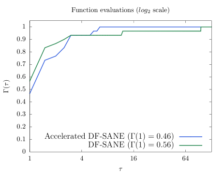
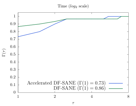
Figure 1: Performance profiles of Accelerated DF-SANE and DF-SANE considering the 30 problems from the CUTEst collection in which both methods found a solution.

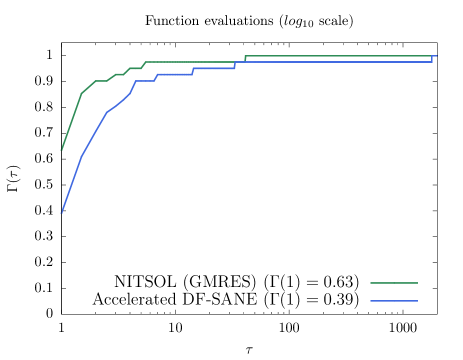
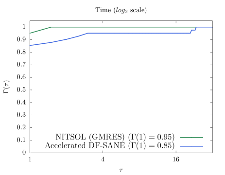
Figure 2: Performance profiles of Accelerated DF-SANE (in Fortran) and NITSOL (GMRES) considering the 41 problems from the CUTEst collection in which both methods found a solution.

In a second experiment, in order to put our method in perspective relatively to a method that represents the state of the art in solving nonlinear systems, we compared Accelerated DF-SANE with NITSOL (GMRES). Since NITSOL (GMRES) is coded in Fortran, we considered the Fortran version of Accelerated DF-SANE in this comparison. Of course, we considered NITSOL (GMRES) without Jacobians. Table LABEL:accvsnitsol and Figure 2 show the results. As in Table LABEL:accvsravi, in column $\|F(x_{*})\|_{2}$, figures in red are the ones that do not satisfy (4). In all cases the final iterate of NITSOL (GMRES) does not satisfy (4), NITSOL (GMRES) stops by “too small step in a line search” (flag equal to 6).

Figures in Table LABEL:accvsnitsol show that both Accelerated DF-SANE and NITSOL (GMRES) solve 45 problems. There are 41 problems that were solved by both methods, 4 problems that were solved by Accelerated DF-SANE only, and 4 problems that were solved by NITSOL (GMRES) only. So, both methods appear to be equally robust.

As well as Figure 1, Figure 2 focuses on efficiency and, thus, it considers only the 41 problems in which both, Accelerated DF-SANE and NITSOL (GMRES), found a solution. Figure 2(a) considers number of functional evaluations as performance metric; while Figure 2(b) considers CPU time. Figure 2(a) shows that NITSOL (GMRES) used less functional evaluations in 63% of the problems; while Accelerated DF-SANE used less functional evaluations in 39% of the problems. (The sum of the percentages is slightly larger than 100% because ties are counted twice.) The fact that the two curves reach 0.9 before $\tau=10$ means that in 90% of the problems the number of function evaluations is of the same order. The Accelerated DF-SANE curve reaches the value 1 for $\tau>1000$ due to only 3 problems. In the problems Recipe, Heart8 and Hatfldg, Accelerated DF-SANE consumes approximately 14, 33 and 1790 times more function evaluations than NITSOL (GMRES). On the other hand, the curve of NITSOL (GMRES) reaches the value 1 between $\tau=10$ and $\tau=100$ because in the problem Waysea1ne NITSOL (GMRES) uses 41 times more function evaluations than Accelerated DF-SANE.

The performance profile of the Figure 2(b) that considers CPU time as performance measure, shows a similar scenario, contaminated by the fact of having a large proportion of small problems. The figure says that NITSOL (GMRES) is the fastest method in 95% of the problems; while Accelerated DF-SANE is the fastest method in 85% of the problems, i.e., there are a lot of ties. (As it can be observed in Table LABEL:accvsnitsol, approximately 90% of the CPU times associated with problems that are solved by both methods are smaller than 0.1 seconds; and CPU times smaller than 0.01 seconds are considered ties.) The curve of NITSOL (GMRES) reaches 1 before $\tau=2$ because in no problem does NITSOL (GMRES) uses more than twice the time of Accelerated DF-SANE. Accelerated DF-SANE also did not use more than twice the time of NITSOL in 37 out of the 41 problems. On the remaining 4 problems, Accelerated DF-SANE uses a little more than twice as much time on Chandheu and Oscigrne (which is why the curve passes 0.95 before $\tau=3$) and on problems Heart8 and Hatfldg it uses 21 and 23 times as much time.

Summing up, we conclude that, while both methods are equally robust, NITSOL (GMRES) is slightly more efficient that Accelerated DF-SANE in the considered set of problems. On the other hand, it is worth noticing that numerical experiments in [3] showed that Accelerated DF-SANE outperforms NITSOL (GMRES) to a large extent on an important class of large-scale problems coming from the discretization of partial differential equations. Of course, the opposite situation can also occur, which justifies the availability of both methods.

Table 2: Detailed results of the application of Accelerated DF-SANE (in Fortran) and NITSOL (GMRES) to the 70 considered problems from the CUTEst collection.

Problem	$n$	Accelerated DF-SANE					NITSOL (GMRES)
		$\|F(x_{*})\|$	# iter	# feval	time		$\|F(x_{*})\|$	# iter	# feval	time
BOOTH	2	$9.9$E$-16$	2	7	0.000014		$4.6$E$-09$	3	8	0.000039
CLUSTER	2	$8.3$E$-07$	23	108	0.000048		$1.2$E$-09$	9	25	0.000046
CUBENE	2	$4.0$E$-13$	9	20	0.000022		$2.1$E$-10$	38	108	0.000076
DENSCHNCNE	2	$2.3$E$-11$	10	23	0.000029		$6.7$E$-07$	6	15	0.000043
DENSCHNFNE	2	$2.7$E$-07$	7	23	0.000019		$1.6$E$-13$	5	16	0.000044
FREURONE	2	$1.5$E$-08$	16	55	0.000025		$7.0$E$+00$	16	112	0.000058
GOTTFR	2	$1.3$E$-07$	23	67	0.000031		$3.6$E$-09$	70	236	0.000133
HIMMELBA	2	$0.0$E$+00$	2	7	0.000013		$2.5$E$-08$	3	8	0.000042
HIMMELBC	2	$8.4$E$-08$	5	13	0.000018		$1.1$E$-06$	6	14	0.000041
HIMMELBD	2	$2.4$E$+00$	11577102	439522728	180.000000		$2.4$E$+00$	48	246	0.000164
HS8	2	$4.4$E$-08$	5	13	0.000018		$2.4$E$-11$	11	24	0.000045
HYPCIR	2	$8.7$E$-10$	6	14	0.000017		$5.2$E$-07$	5	13	0.000041
POWELLBS	2	$1.4$E$-06$	54229896	1259707609	152.775132		$1.9$E$-06$	231	692	0.000206
POWELLSQ	2	$1.4$E$-00$	13690098	34211713	180.000000		$1.3$E$+00$	37498	309809	0.044447
PRICE3NE	2	$3.9$E$-10$	7	19	0.000020		$4.4$E$-10$	7	20	0.000046
PRICE4NE	2	$1.3$E$-10$	10	27	0.000030		$3.0$E$-09$	10	27	0.000048
RSNBRNE	2	$2.2$E$-16$	56	204	0.000054		$1.4$E$-06$	55	161	0.000075
SINVALNE	2	$4.9$E$-15$	16	77	0.000040		$1.9$E$-14$	6	19	0.000042
WAYSEA1NE	2	$1.3$E$-10$	12	36	0.000023		$3.4$E$-08$	331	1485	0.000291
WAYSEA2NE	2	$8.4$E$-07$	481	2179	0.000401		$1.3$E$-09$	766	3751	0.000677
DENSCHNDNE	3	$2.3$E$-07$	26	62	0.000043		$1.5$E$-06$	22	71	0.000065
DENSCHNENE	3	$9.6$E$-11$	6	16	0.000032		$1.5$E$-09$	7	19	0.000046
HATFLDF	3	$1.4$E$-08$	26	78	0.000049		$9.6$E$-07$	71	233	0.000117
HATFLDFLNE	3	$7.9$E$-03$	11587628	252488903	180.000000		$7.8$E$-03$	372	2843	0.000672
HELIXNE	3	$2.8$E$-09$	13	35	0.000045		$5.0$E$+01$	0	14	0.000040
HIMMELBE	3	$9.7$E$-16$	9	21	0.000023		$7.3$E$-09$	2	9	0.000043
RECIPE	3	$6.2$E$-07$	72	403	0.000116		$1.4$E$-06$	10	28	0.000048
ZANGWIL3	3	$1.4$E$-14$	3	11	0.000015		$5.2$E$-07$	3	10	0.000045
POWELLSE	4	$7.3$E$-07$	24	70	0.000061		$1.5$E$-06$	13	61	0.000064
POWERSUMNE	4	$1.2$E$-02$	8695243	130633973	180.000000		$1.6$E$-06$	1417	7084	0.004665
HEART6	6	$1.5$E$-06$	124382	1818751	0.561869		$2.7$E$-01$	3854	28811	0.013372
HEART8	8	$2.8$E$-06$	181971	2866905	0.993949		$2.2$E$-06$	11360	86495	0.046512
COOLHANS	9	$1.5$E$-06$	10	45	0.000056		$2.3$E$-06$	7	22	0.000057
MOREBVNE	10	$1.6$E$-06$	37	219	0.000124		$7.9$E$-08$	4	33	0.000068
OSCIPANE	10	$1.0$E$+00$	8608149	322784536	180.000000		$1.0$E$+00$	2411	50650	0.022718
TRIGON1NE	10	$1.9$E$-06$	13	29	0.000063		$2.5$E$-06$	5	26	0.000069
INTEQNE	12	$9.2$E$-07$	3	7	0.000021		$3.3$E$-07$	4	10	0.000065
HATFLDG	25	$5.0$E$-06$	22708	356246	0.232828		$7.8$E$-07$	44	199	0.000263
HYDCAR6	29	$5.0$E$-03$	2661134	61551663	180.000000		$3.3$E$-01$	30	781	0.002596
METHANB8	31	$1.2$E$-04$	2577703	67500153	180.000000		$1.4$E$-02$	6	472	0.001542
METHANL8	31	$4.4$E$-03$	2764968	66380772	180.000000		$6.1$E$-01$	28	1052	0.003356
HYDCAR20	99	$3.9$E$-02$	917448	19172981	180.000000		$9.2$E$+00$	3	287	0.003190
LUKSAN21	100	$8.9$E$-06$	48	441	0.001177		$6.1$E$-06$	17	123	0.000562
MANCINONE	100	$5.9$E$-07$	5	17	0.009272		$3.9$E$-06$	4	11	0.005929
QINGNE	100	$4.8$E$-06$	21	45	0.000233		$4.3$E$-06$	10	35	0.000150
ARGTRIG	200	$1.2$E$-05$	57	199	0.016417		$1.1$E$-05$	5	86	0.007244
BROWNALE	200	$1.0$E$-05$	9	25	0.001325		$3.1$E$-07$	3	9	0.000512
CHANDHEU	500	$1.4$E$-05$	18	99	0.140877		$1.5$E$-05$	10	51	0.065100
10FOLDTR	1000	$2.2$E$+07$	9445	272830	180.000000		$2.7$E$-05$	54	6563	4.562871
KSS	1000	$9.3$E$-06$	5	17	0.023044		$2.2$E$-08$	6	13	0.017676
MSQRTA	1024	$4.7$E$+01$	68938	1137480	180.000000		$5.5$E$+01$	17	1351	0.210034
MSQRTB	1024	$4.6$E$+01$	61153	1138024	180.000000		$5.9$E$+01$	13	1964	0.306907
EIGENAU	2550	$1.6$E$+02$	12625	234607	180.000000		$1.6$E$+02$	17	850	0.768981
EIGENB	2550	$9.6$E$+00$	15297	234454	180.000000		$9.8$E$+00$	9	382	0.361665
EIGENC	2652	$9.2$E$+01$	14864	218919	180.000000		$9.7$E$+01$	33	2169	2.097641
NONMSQRTNE	4900	$2.4$E$+02$	5731	85005	180.000000		$2.3$E$+02$	23	915	1.804071
BROYDN3D	5000	$5.3$E$-05$	12	25	0.005502		$2.8$E$-05$	5	19	0.002987
BROYDNBD	5000	$2.4$E$+00$	58861	934685	180.000000		$7.7$E$+00$	11	607	0.176834
BRYBNDNE	5000	$2.4$E$+00$	57595	915686	180.000000		$7.7$E$+00$	11	607	0.176482
NONDIANE	5000	$1.0$E$+00$	83049	1603628	180.000000		$6.1$E$+02$	686	10094	1.873028
SBRYBNDNE	5000	$2.5$E$+02$	45364	906538	180.000000		$2.7$E$+02$	50	2935	0.918074
SROSENBRNE	5000	$2.5$E$-09$	9	34	0.004332		$2.1$E$-08$	4	11	0.001462
SSBRYBNDNE	5000	$1.7$E$+02$	50681	944507	180.000000		$1.6$E$+02$	128	9043	2.794424
TQUARTICNE	5000	$8.3$E$-01$	175237	1886434	180.000000		$1.5$E$-07$	2	6	0.000899
OSCIGRNE	100000	$1.8$E$-04$	28	66	0.461298		$1.5$E$-04$	7	34	0.158588
CYCLIC3	100002	$6.2$E$-01$	3011	53186	180.000000		$1.7$E$-04$	282	992	4.070610
YATP1CNE	123200	$2.6$E$-07$	14	41	0.889454		$1.4$E$-04$	17	48	0.970848
YATP1NE	123200	$2.6$E$-07$	14	41	0.891586		$1.4$E$-04$	17	48	0.974741
YATP2CNE	123200	$3.1$E$+04$	800	12314	180.000000		–	–	–	180.000000
YATP2SQ	123200	$4.1$E$+04$	791	12362	180.000000		–	–	–	180.000000

A side note comparing the R and Fortran implementations of Accelerated DF-SANE is in order. Comparing Tables LABEL:accvsravi and LABEL:accvsnitsol, it can be seen that they deliver slightly different results in a few problems and deliver identical results in 40 problems out of the 44 problems in which none of the versions stops by reaching the CPU time limit. If we consider these 40 problems, in which both versions performed an identical number of iterations and functional evaluations, the Fortran version uses, in average, around 10% of the CPU time required by the R version of the method.

5 Conclusions

In [3], where it was shown that an acceleration scheme based on the Sequential Secant Method could improve the performance of the derivative-free spectral residual method [13], numerical experiments with very large problems coming from the discretization of partial differential equations were presented. In the considered family of problems, Accelerated DF-SANE outperformed DF-SANE and NITSOL (GMRES) by a large extent.

In the present work, an R implementation of the method proposed in [3] was introduced. In addition, numerical experiments considering all nonlinear systems of equations from the well-known CUTEst collection were presented. Default dimensions of the problems were considered; and the collection includes small-, medium-, and large-scale problems. Results shown that the proposed method is much more robust than the DF-SANE method included in the R package BB [21]; while it is as robust and almost as efficient as the state-of-the-art classical NITSOL (GMRES) method (coded in Fortran). Therefore, the proposed method appears as a useful and robust alternative for solving nonlinear systems of equations without derivatives to the users of R language.

As a byproduct, an interface to test derivative-free nonlinear systems solvers developed in R with the widely-used test problems from the CUTEst collection [11] was also provided.

References

- [1] J. G. P. Barnes. An algorithm for solving nonlinear equations based on the secant method. The Computer Journal, 8(1):66–72, 1965.
- [2] J. Barzilai and J. M. Borwein. Two-point step size gradient methods. IMA Journal of Numerical Analysis, 8(1):141–148, 1988.
- [3] E. G. Birgin and J. M. Martínez. Secant acceleration of sequential residual methods for solving large-scale nonlinear systems of equations. Technical Report arXiv:2012.13251v1, arXiv, 2021.
- [4] E. G. Birgin, J. M. Martínez, and M. Raydan. Nonmonotone spectral projected gradient methods on convex sets. SIAM Journal on Optimization, 10(4):1196–1211, 2000.
- [5] E. G. Birgin, J. M. Martínez, and M. Raydan. Algorithm 813: Spg – software for convex-constrained optimization. ACM Transactions on Mathematical Software, 27(3):340–349, 2001.
- [6] E. G. Birgin, J. M. Martínez, and M. Raydan. Spectral projected gradient methods. In C. A. Floudas and P. M. Pardalos, editors, Encyclopedia of Optimization, pages 3652–3659. Springer US, Boston, MA, 2009.
- [7] E. G. Birgin, J. M. Martínez, and M. Raydan. Spectral projected gradient methods: Review and perspectives. Journal of Statistical Software, 60(3), 2014.
- [8] R. H. Byrd, P. Lu, and J. Nocedal. A limited memory algorithm for bound constrained optimization. SIAM Journal on Scientific and Statistical Computing, 16(5):1190–1208, 1995.
- [9] A. R. Conn, N. I. M. Gould, and Ph. L. Toint. Lancelot – A Fortran Package for Large-Scale Nonlinear Optimization (Release A). Springer, Berlin, Heidelberg, 1992.
- [10] E. D. Dolan and J. J. Moré. Benchmarking optimization software with performance profiles. Mathematical Programming, 91(2):201–213, 2002.
- [11] N. I. M. Gould, D. Orban, and Ph. L. Toint. CUTEst: a Constrained and Unconstrained Testing Environment with safe threads for mathematical optimization. Computational Optimization and Applications, 60(3):545–557, 2015.
- [12] W. Hock and K. Schittkowski. Test Examples for Nonlinear Programming Codes, volume 187 of Lecture Notes in Economics and Mathematical Systems. Springer, Berlin, Heidelberg, 1981.
- [13] W. La Cruz, J. M. Martínez, and M. Raydan. Spectral residual method without gradient information for solving large-scale nonlinear systems of equations. Mathematics of Computation, 75:1429–1448, 2006.
- [14] W. La Cruz and M. Raydan. Nonmonotone spectral methods for large-scale nonlinear systems. Optimization Methods and Software, 18(5):583–599, 2003.
- [15] J. J. Moré, B. S. Garbow, and K. E. Hillstrom. Testing unconstrained optimization software. ACM Transactions on Mathematical Software, 7(1):17–41, 1981.
- [16] M. Pernice and H. F. Walker. NITSOL: a newton iterative solver for nonlinear systems. SIAM Journal on Scientific Computing, 19(1):302–318, 1998.
- [17] M. Raydan. On the barzilai and borwein choice of steplength for the gradient method. IMA Journal of Numerical Analysis, 13(3):321–326, 1993.
- [18] M. Raydan. The barzilai and borwein gradient method for the large scale unconstrained minimization problem. SIAM Journal on Optimization, 7(1):26–33, 1997.
- [19] K. Schittkowski. More Test Examples for Nonlinear Programming Codes, volume 282 of Lecture Notes in Economics and Mathematical Systems. Springer, Berlin, Heidelberg, 1987.
- [20] The R Core Team. R: A Language and Environment for Statistical Computing. R Foundation for Statistical Computing, Vienna, Austria, 2009.
- [21] R. Varadhan and P. Gilbert. BB: An R package for solving a large system of nonlinear equations and for optimizing a high-dimensional nonlinear objective function. Journal of Statistical Software, 32(4):1–26, 2009.
- [22] P. Wolfe. The secant method for simultaneous nonlinear equations. Communications of ACM, 2(12):12–13, 1959.