Self-supervised Spatial Reasoning on Multi-View Line Drawings

Abstract

Spatial reasoning on multi-view line drawings by state-of-the-art supervised deep networks is recently shown with puzzling low performances on the SPARE3D dataset [han2020spare3d]. Based on the fact that self-supervised learning is helpful when a large number of data are available, we propose two self-supervised learning approaches to improve the baseline performance for view consistency reasoning and camera pose reasoning tasks on the SPARE3D dataset. For the first task, we use a self-supervised binary classification network to contrast the line drawing differences between various views of any two similar 3D objects, enabling the trained networks to effectively learn detail-sensitive yet view-invariant line drawing representations of 3D objects. For the second type of task, we propose a self-supervised multi-class classification framework to train a model to select the correct corresponding view from which a line drawing is rendered. Our method is even helpful for the downstream tasks with unseen camera poses. Experiments show that our method could significantly increase the baseline performance in SPARE3D, while some popular self-supervised learning methods cannot.

1 Introduction

Human visual reasoning, especially spatial reasoning, has been widely studied from psychological and educational perspectives [kell2013creativity, hsi1997role]. Researches show that trained humans can achieve good performance on spatial reasoning tasks [ramful2017measurement] because they can solve these tasks using spatial memory, logic, and imagination. However, the spatial reasoning of deep networks is yet to be explored and improved. In other visual learning tasks such as image classification, object detection, and segmentation, state-of-the-art deep networks have shown their superior performance to humans by memorizing indicative visual patterns from enormous image instances for prediction. However, it seems difficult for deep networks to reason using the same mechanism about the spatial information such as the view consistency and camera poses from 2D images [han2020spare3d].

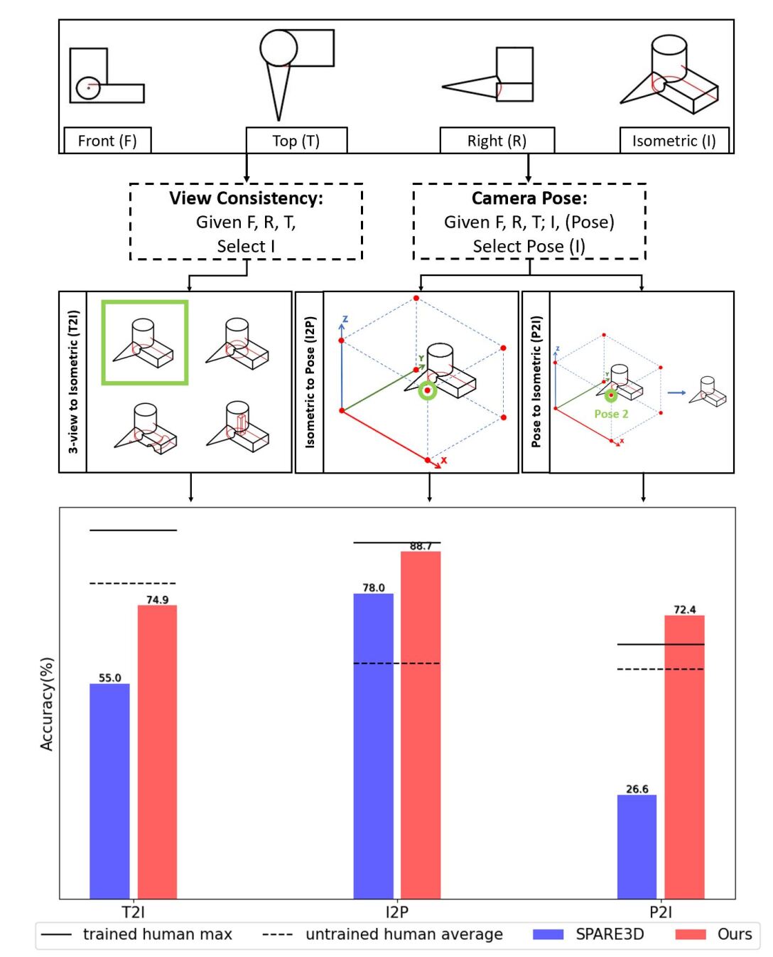
Figure 1: We significantly improve SPARE3D baselines using self-supervised learning approaches. Note that in this figure, all the networks are trained using the same amount of data (data generated from 5,000 CAD models) as used on the SPARE3D dataset.

To our best knowledge, we are the first to investigate spatial reasoning tasks in the SPARE3D dataset [han2020spare3d], that provides several challenging spatial reasoning tasks in line drawings (Figure 1). The dataset is unique in that: (1) it uses line drawings as inputs, (2) it is a non-categorical dataset, meaning there is no class label information for each object, (3) it defines spatial reasoning instead of recognition tasks. Specifically, we focus on the view-consistency reasoning task (the Three-view to Isometric or T2I) and the two camera-pose reasoning tasks (the Isometric to Pose or I2P, and the Pose to Isometric or P2I). The task examples are illustrated in Figure 1 and for more details of the task settings, we refer the readers to the SPARE3D paper [han2020spare3d].

To improve the DNN’s performance, our first effort is to explore the supervised learning network’s ability in three aspects: (1) the quantity of data used for learning, (2) the network’s capacity (width and depth), and (3) the network’s structure. However, we find changing these factors could not bring significant improvement (all these results are shown in the supplementary), while it might cost more time and computational resources to generate data for supervised learning.

Compared with supervised learning, self-supervised learning is helpful when a large number of unlabeled data are available. Moreover, in many visual learning tasks, self-supervised learning as a pre-training task can learn better visual representations that can be further fine-tuned via supervision for downstream tasks, achieving similar or even better results than supervised learning [chen2020big]. Based on these findings, we design two self-supervised learning methods for both view consistency reasoning task and camera pose reasoning task on the SPARE3D dataset.

For the view consistency reasoning task, we design a contrastive spatial reasoning method to tackle the challenges in SPARE3D tasks (Figure 2). This is necessary because most of the existing contrastive learning methods do not explicitly consider the relationship between different views, nor do they force deep networks to focus on detailed differences between images. We demonstrate both qualitative and quantitative results that show our method helps deep networks capture these small details while being view invariant, which is crucial for the view consistency task.

For the camera pose reasoning task, we propose a self-supervised learning network for improving the deep network’s ability to find the correlation between the pose and the image rendered from the pose (see Figure 6). Our experiment results show that our self-supervised learning network is not only helpful for the downstream tasks with seen views but also helpful for the tasks with unseen views. This shows a potential to even improve pose estimation by transferring the learned representations from a camera pose reasoning pretext task to related downstream tasks.

In sum, our major contributions are:

• A novel contrastive learning method by self-supervised binary classifications, which enables deep networks to effectively learn detail-sensitive yet view-invariant multi-view line drawing representations for view consistency reasoning task;

• A self-supervised multi-class classification method to learn pose-aware representations from multi-view line drawing images;

• Significantly improved spatial reasoning performance of deep networks on line drawings based on the above, some of which surpass human performance.

2 Related Work

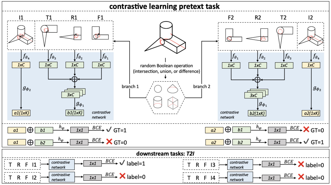
Figure 2: Contrastive spatial reasoning architecture for task T2I. We train a contrastive learning network, then use the learned representations to the downstream task T2I. Front (F), Right (R), Top (T) represent line drawings and an isometric (I) line drawing. $a_{1},b_{1},a_{2},b_{2}$ are the encoded feature vectors; $C$, $K$ are the dimension of the latent vectors. The $f_{\theta_{1}}$, $f_{\theta_{2}}$, $f_{\theta_{3}}$, and $f_{\theta_{4}}$ are CNN networks; $g_{\phi_{1}}$, $g_{\phi_{2}}$, and $h_{\psi}$ are MLP networks. $\bigoplus$ is a concatenation operation. BCE represents binary cross-entropy loss.

Self-supervised learning has achieved great success due to the performance improvement on many visual learning tasks [godard2019digging, misra2020self, kim2020spatially, wang2020self, zhai2019s4l, kolesnikov2019revisiting, you2022class, jing2020self, goyal2019scaling, liu2021auto]. Successful self-supervised learning frameworks use different tricks to create artificial labels based solely on the inputs. One way is to use spatial information or spatial relationships between image patches in a single image. For example, gidaris2018unsupervised designed the pretext task by asking the network to predict image rotations. Another way is to ask the network to recover the positions of shuffled image patches [kim2018learning, noroozi2016unsupervised, wei2019iterative], or predict the relative position [doersch2015unsupervised]. In addition, the color signal contained in an RGB image could also be used. By recovering the color for grayscale images generated from RGB images, networks can learn the semantic information of each pixel [zhang2016colorful, larsson2016learning]. Despite the success of the spatial reasoning tasks in the SPARE3D dataset, these methods are ineffective since they only use visual information from a single image. Our method aims to consider the common information between different images and, thus, is more suitable to solve those reasoning problems.

One way of grouping various self-supervised learning methods is to divide them into generative vs. contrastive ones [liu2020self]. On the one hand, generative ones learn visual representations via pixel-wise loss computation and thus forcing a network to focus on pixel-based details; on the other hand, contrastive ones learn visual representations by contrasting the positive and negative pairs [anand2020contrastive, you2021momentum, you2021simcvd, you2021self]. Many researchers explored contrastive learning by comparing shared information between multiple positive or negative image pairs. These methods often attempt to minimize the distance of the features extracted from the same data source and maximize the distance between features from different data sources in the feature space. hjelm2018learning propose Deep InfoMax based on the idea that the global feature extracted from an image should be similar to the same image’s local feature and should be different from a different image’s local feature. Based on this method, bachman2019learning further use image features extracted from different layers to compose more negative or positive image pairs. SimCLR [chen2020simple] differs from the previous two methods in that it only considers the global features of the augmented image pairs to compose positive and negative pairs. SimCLRv2 [chen2020big] make further improvements on Imagenet [deng2009imagenet] by conducting contrastive learning with a large network, fine-tuning using labeled data, and finally distilling the network to a smaller network. Compared to SimCLR, MoCo [he2020momentum] stores all generated samples to a dictionary and uses them as negative pairs instead of generating negative pairs in each step. These tactics could help reduce the batch size requirement while still achieving good performance. Differently, SwaV [caron2020unsupervised] trains two networks that can interact and learn from each other, with one network’s input being the augmented pair of another network’s input. Besides, researchers also theoretically analyze why these contrastive learning methods work well [arora2019theoretical, tosh2020contrastive, lee2020predicting, tian2020understanding].

However, it is difficult to apply the aforementioned contrastive learning methods directly to tasks which requires consideration of the relationships between multi-view images. Contrastive multiview coding [tian2019contrastive] has a misleading name in our context because that “multiview” in fact, means different input representations instead of views from different camera poses. Therefore it is not suitable for SPARE3D tasks. kim2020few propose a method to solve a few-shot visual reasoning problem on RAVEN dataset [zhang2019raven], which is perhaps more relevant to us due to the use of contrastive learning in visual reasoning. Yet because it is designed for analogical instead of spatial reasoning, it is not directly applicable to SPARE3D tasks either.

3 What Affects SPARE3D Performance?

To better understand the SPARE3D tasks and why state-of-the-art deep networks have low performances, we study three potentially relevant factors: CAD model complexity, network capacity, and network structure respectively. For each factor, we first give a natural hypothesis about its influence on SPARE3D baseline performance. Then, we design controlled experiments to prove or disprove the hypothesis and finally obtain heuristics about both the causes of the existing baseline’s low performance and potentially more effective network designs.

Controlled experiment settings. For investigating the CAD model complexity and the network capacity factors, we focus on the view-consistency reasoning (T2I) and the camera-pose reasoning (I2P) tasks on SPARE3D-ABC dataset. For the network structure factor, we use both the T2I, the I2P, and the P2I tasks. We follow the same baseline settings as in [han2020spare3d]: for T2I and P2I tasks, we use the binary classification baseline networks; for I2P task, we use the multi-class classification baseline network. The backbone network for these baseline networks are VGG-16 [simonyan2014very]. We select these baseline networks since they are the best performing ones in [han2020spare3d]. All experiments are implemented using PyTorch [PyTorch:NIPS19] and conducted on NVIDIA GeForce GTX 1080 Ti GPU. For each experiment, we tune the hyperparameters to seek the best performance (details in the supplementary material).

3.1 CAD model complexity

Motivation: we want to study if the level of CAD model complexity affects the baseline performance for SPARE3D tasks. It is discussed in [murty1999evaluating] that the complexity of a CAD task is associated with its difficulty for humans. However, the relationship between the CAD model complexity and the difficulty level for deep networks to solve the spatial reasoning tasks has not been fully studied. To study the influence of CAD model complexity for deep networks, we use the number of primitives in CAD models to represent the complexity of CAD models, as discussed in [murty1999evaluating]. In practice, we use the constructive solid geometry (CSG) modeling method to generate the dataset with different numbers of primitives yet fixed primitive types and boolean operations. With the increasing number of primitives of the CSG models, the level of CAD complexity also increases.

Hypothesis 1: the higher level of CAD model complexity will cause lower SPARE3D baseline network performance, as long as the corresponding line drawings are still visually legible for the reasoning tasks.

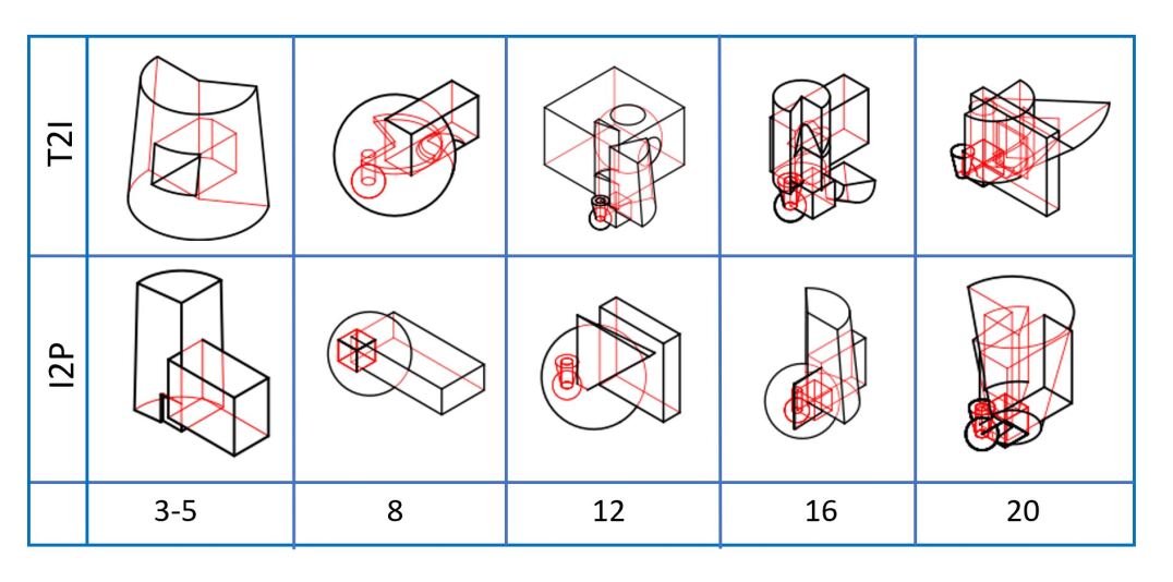
Figure 3: CSG models with different number of primitives.

Experiment details. We use FreeCAD [riegel2016freecad] to generate a CSG model dataset with a various number of primitives. We follow the generation settings as in [han2020spare3d]. The primitives used are sphere, cube, cone, and cylinder; the Boolean operations used are intersection, union, and difference. For both the task T2I and I2P, we generate seven groups of CSG models, with primitive number 3-5, $8$, $12$, $16$, $20$, $24$, and $30$. The 3-5 means the number of primitives making up a CAD model is $3$, $4$, or $5$. For each group, it has $4000$ models for training and $500$ models for testing. Exemplar line drawings rendered with CAD models composed of a different number of primitives can be seen in Figure 3. We can see that the models become visually more complex when the number of primitives increases.

Experiment results. Figure 4 left shows that for the T2I task, in general, the more primitives a CSG model has, the lower the testing accuracy is, as expected in Hypothesis 1. The results for the primitive-number $12$ and $20$ are just minor variations in the experiments, which are most likely caused by the data randomness. We think it is because when the number of primitives increases, the lines in the line drawings become denser; therefore, it is more difficult for a network to distinguish the tiny difference between candidate line drawings (see the exemplar candidate answers in Figure 1). Thus, we call T2I the detail-hurt task.

However, unexpected results are shown in Figure 4 right, where the accuracy increases first and then decreases after the primitive number becomes more than 20. We believe it is because, within a certain range of CAD complexity, the more primitives the CAD model contains, the more visual features a network can extract for camera-pose reasoning, thus the higher testing accuracy. However, if a CAD model is too complex, the line drawings become too crowded to provide effective feature extraction and reasoning.

We then notice that the CAD models in the SPARE3D-ABC dataset are mostly from the real world, and their complexity level is close to the CSG models with typically less than $20$ primitives. Therefore, for the SPARE3D-ABC dataset, we think more shape details can help a network in camera-pose reasoning, which we call a detail-help task.

Heuristics 1: the experiment results show our hypothesis is not completely correct. Indeed, more shape details help the camera-pose tasks on the SPARE3D-ABC dataset but hurt the view-consistency task. Therefore, we may need different methods for them, respectively, and an effective method for T2I task should be detail-sensitive to capture detailed differences between candidate answers.

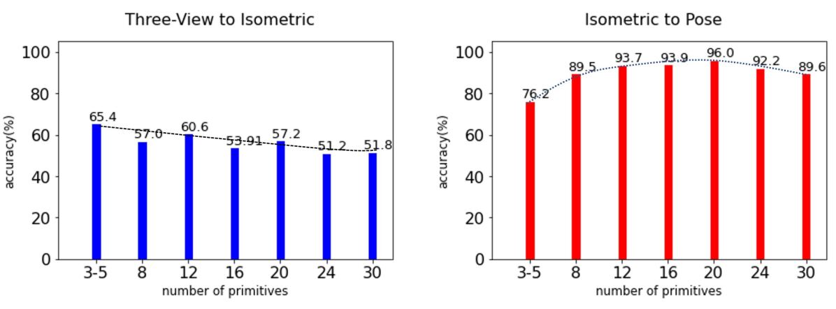
Figure 4: CAD model complexity vs. test accuracy.

3.2 Network capacity

Motivation: we want to study if the network’s capacity will affect the baseline performance for tasks on SPARE3D-ABC. Using a large (over-parameterized) network is widely used to achieve better performance on some deep learning tasks [huang2019gpipe, tan2019efficientnet]. To increase a network’s capacity, we can make the network deeper or wider without making changes to other components in the network.

Hypothesis 2: a baseline network’s performance will improve if the network’s capacity increases.

Experiment details. With the VGG-16 network as a backbone, we define the width of the network as the width of the last convolutional layer (the number of output channels). By this definition, the width of the VGG-16 network in [han2020spare3d] is $512$. In the comparative experiments, we change the width to $384$, $448$, and $1024$. The width of other convolutional layers is proportionally adapted to the final convolutional layer’s width, ensuring the network’s widths are changed gradually. Detailed widths of each layer for the VGG-16 backbone network with different widths can be found in the supplementary. The depth of the network represents the number of layers of the VGG family backbone networks. We use VGG-13, VGG-19 based backbone as in [simonyan2014very] to represent three different depths of the network.

Figure 5: Network capacity (width and depth) vs. test accuracy. The results show that naively increasing the network capacity cannot improve the network performance on T2I and I2P tasks.

Experiment results. For task T2I, decreasing the network’s width does not hurt the network’s performance, although strangely, increasing the network’s width leads to a decrease in the testing accuracy (Figure 8 top-left). We think it is because the network with more parameters requires more data, and using the same amount of data to train networks with different widths is insufficient. For the depth control experiments, we find almost no differences among the three selected network depth values (Figure 8 top-right). For task I2P, neither the width nor the depth of the network can significantly improve the network’s performance(Figure 8 bottom).

Heuristics 2: our hypothesis is incorrect. In fact, merely increasing network capacities cannot improve the baseline’s performances. Therefore, to improve SPARE3D performance, we need new networks or losses than only supervised classification networks with larger capacities.

3.3 Network structure

Motivation: we want to study if the network’s structure can affect the baseline performance for tasks on SPARE3D-ABC. Changing the structure of the network is a potential way to improve the accuracy of some deep learning tasks, e.g., one famous example is to use the residual links in deep networks [he2016deep]. To find a proper structure for the view-consistency reasoning task (T2I) and camera-pose reasoning tasks (I2P and P2I), we tried a lot of variants of the backbone network (all variants and the corresponding results will be shown in supplementary). We also test whether the network’s performance will change if using the pre-trained parameters on Imagenet [deng2009imagenet], inspired by [funke2020notorious].

Hypothesis 3: for each SPARE3D task, a baseline network’s performance will improve if we find a more proper network structure and parameter initialization.

Experiment details. We find two changes on the network that will have a consistent impact on the network’s performance for all SPARE3D tasks: one is whether the network’s parameters are initialized using Imagenet pre-trained parameters; another one is whether the three-view drawings (front view, right view, and top view drawings) and isometric drawings are fed to separate and independent branches of the network. We call the second one late fusion.

Early fusion vs. late fusion. In the original SPARE3D paper [han2020spare3d], the baseline backbone network treats all the input images (front, right, top view drawings, and one isometric view drawing from the candidate answers) as a whole, and it concatenates those images before sending them to the first convolutional layer. We call this way of feeding multi-view line drawings to a network as the early fusion. In contrast, we design a network that takes the three-view drawings and the isometric view drawing as separate inputs, which means the input drawings are sent to a convolutional network that shares the same architecture yet has separate network parameters. We name this way of separately handling the input as the late fusion since the extracted image features are concatenated later. Other network structures are kept the same as the baseline method in [han2020spare3d]. Therefore, we have four experiments, which are the combination of training the network with/without Imagenet pre-trained parameters and using early fusion or late fusion.

For the P2I task, we make an extra modification of the network in the baseline method. In the original baseline method, after extracting the input images’ feature vector, the feature vector is concatenated with an 8-dimensional one-hot camera-pose code. Then the concatenated vector is sent to a fully connected layer to obtain a classification probability distribution. Differently, our method extracts the feature of the composite images (F, R, T, and a candidate isometric view image) into an 8-dimensional vector as the camera-pose probability logits of the candidate isometric view. Then we select the logit corresponding to the given pose to compute the cross-entropy loss. We find this minor modification can effectively improve the network’s performance on the P2I task. The modification details will be given in the supplementary.

Experiment results. As shown in Table 1, we find that using pre-trained parameters and the late fusion can improve the network’s performance on camera-pose reasoning tasks (I2P and P2I). By using these tactics, the accuracy of I2P and P2I achieves $85.4\%$ and $72.4\%$ respectively, which is already higher than the baseline in SPARE3D. However, the same tactics turned out to decrease the network’s performance on T2I task significantly. We leave these puzzling results for our future investigations.

Table 1: Network architecture vs. performance. We test four conditions, considering 1) using Imagenet pre-trained parameters or not, 2) using late fusion method or early fusion method. “y/n” indicates using the network structure or not. P2I task uses the slightly improved network structure as previously explained.

pre-train	late fusion	T2I	I2P	P2I
n	n	55.0	78.0	64.0
n	y	22.8	80.0	66.6
y	n	30.6	80.4	68.6
y	y	25.2	85.4	72.4

Heuristics 3: based on above results, we believe: 1) a proper parameter initialization can improve baseline performances; 2) using late fusion or early fusion will affect baseline performances, yet the impact depends on the task. Therefore, for task T2I, whose baseline performance is relatively lower than I2P and P2I (see row 1 of Table 1), we still need a better method. In the next section, we will design a specialized contrastive learning method using all the above heuristics to improve the SPARE3D T2I baseline.

4 Self-supervised Spatial Reasoning

In this section, we explore a self-supervised learning method to learn the representations for all three tasks in SPARE3D: a contrastive spatial reasoning network for view consistency reasoning task T2I, a self-supervised learning network for camera pose reasoning task I2P and P2I. For the camera pose reasoning task, we extend the downstream task settings to show our method is helpful when the camera poses in the downstream task are not seen in the pretext task.

4.1 Contrastive learning network for task T2I

According to the discussion in the Introduction 1, we believe contrastive learning can help the network learn better line drawing representations. Because it is not difficult to obtain a large number of unlabeled CAD models, we design our specialized contrastive spatial reasoning method as illustrated in Figure 2. Our method can be divided into three steps: 3D model augmentation, line-drawing feature extraction, contrastive loss computation.

Step 1: 3D data augmentation. Our data augmentation happens in 3D instead of 2D because the visual differences between different views are caused by 3D boolean operation. We generate two sets of images: a branch 1 set and a branch 2 set for each augmented CAD model. Each image set contains the three-view drawings and the isometric view drawing. We denote the branch 1 set by $\left\{F_{1},R_{1},T_{1},I_{1}\right\}$, and the branch 2 set by $\left\{F_{2},R_{2},T_{2},I_{2}\right\}$, where $F$, $R$, $T$, and $I$ stand for front, right, top views and the isometric view separately. The branch 1 and branch 2 image sets are generated from two different modifications to the original CAD model. Each modification is a random Boolean operation (intersection, union, or difference) on the original CAD model with a random primitive (sphere, cube, cone, or cylinder.) Figure 2 gives an example of generating the two image sets.

Step 2: line-drawing feature extraction. In this paper, $f,g,h$ represent neural networks; $\theta,\phi,\psi$ are the network weights in the three networks respectively. $F_{i}$, $R_{i}$, $T_{i}$, and $I_{i}$ ($i\in\{1,2\}$) are fed into four convolutional neural networks (CNN) individually. The four networks are denoted by $f_{\theta_{1}}$, $f_{\theta_{2}}$, $f_{\theta_{3}}$, and $f_{\theta_{4}}$, where $f_{\theta_{j}}:\mathbb{R}^{3\times H\times W}\to\mathbb{R}^{C},j\in\{1,2,3,4\}$; $H$ and $W$ are the height and width of the images. Note that the four networks share the same architecture but with different parameters. Then, the outputs from $f_{\theta_{1}}$, $f_{\theta_{2}}$, and $f_{\theta_{3}}$ are concatenated and fed into a one-layer MLP $g_{\phi_{1}}:\mathbb{R}^{3C}\to\mathbb{R}^{K}$, and the output from $f_{\theta_{4}}$ is fed into another one-layer MLP $g_{\phi_{2}}:\mathbb{R}^{C}\to\mathbb{R}^{K}$. $g_{\phi_{1}},g_{\phi_{2}}$ also share the same architecture but with different parameters. The outputs from $g_{\phi_{1}}$ and $g_{\phi_{2}}$ are noted as a $a_{i}$ and $b_{i}$ ($i\in\{1,2\}$) , which encode the information from the 3-view images and the isometric image respectively.

Step 3: Contrastive loss computation. After having the four latent codes ($a_{1}$, $a_{2}$, $b_{1}$, and $b_{2}$), we concatenate each $a$ and each $b$, which gives four combinations $a_{1}\bigoplus b_{1}$, $a_{1}\bigoplus b_{2}$, $a_{2}\bigoplus b_{1}$, and $a_{2}\bigoplus b_{2}$ (see Figure 2). Then we send the four concatenated latent codes to a binary classifier $h_{\psi}:\mathbb{R}^{2K}\to(0,1)$, where the $h_{\psi}$ is a two-layer MLP. The outputs from $h_{\psi}$ are $\hat{p}_{1}$, $\hat{p}_{2}$, $\hat{p}_{3}$, and $\hat{p}_{4}$ respectively, and are used to compute the binary cross entropy (BCE) loss with the ground truth. We define the ground truth to be $1$ if the original two latent codes used to concatenate are from the same image pairs, and the ground truth to be $0$ from different image pairs. Therefore, $p_{1}=p_{4}=1$, $p_{2}=p_{3}=0$. The final loss is $\frac{1}{4}\sum_{k=1}^{4}BCE(\hat{p}_{k},p_{k})$, ($k\in\{1,2,3,4\}$).

Difference with SimCLR. Unlike existing contrastive learning methods such as SimCLR, the representation from our method is designed to be both multi-view-consistent and detail-sensitive. Technically, our method differs from them in that: 1) our data augmentation operates on 3D CAD models with Boolean operations (intersection, union, or difference), instead of single-image operations like random cropping, color distortion, and Gaussian blur; 2) our positive pairs are two sets of multi-view line drawings (three-view line drawings and isometric line drawing) that are rendered in the same data branch, and our negative pairs are image sets from different data branches, unlike being sampled from other data instances; 3) we use binary cross-entropy loss to optimize the network, unlike the NT-Xent loss [gutmann2010noise, zhang2019learning] which has the temperature parameter to tune. Our experimental results also show the advantage of using BCE loss over the NT-Xent loss.

Representation adaption for task T2I. We notice that all the learned parameters $\theta,\phi,\psi$ can be loaded to the neural network for further supervised fine-tuning because the contrastive spatial reasoning method is just a pre-training step, and it uses exactly the same network architecture as the network for the supervised learning (see Figure 2 downstream tasks: T2I).

4.2 Self-supervised learning network for task I2P and P2I

We propose a self-supervised learning pretext task, as can be seen in Figure 6. As mentioned in Introduction 1, the learned representations from the pretext task can be helpful to both I2P and P2I tasks, even when the camera poses in the downstream tasks are not seen in the pretext task. The network design can be divided into two steps: line-drawing feature extraction; loss computation.

Figure 6: Self-supervised learning network architecture for task I2P and P2I. We train a self-supervised learning network (left subfigure), then use the learned representations to the downstream tasks I2P and P2I (right subfigure). The $f_{\eta_{1}}$, $f_{\eta_{2}}$, $f_{\eta_{3}}$, and $f_{\eta_{4}}$ are CNN networks; $g_{\omega_{1}}$, $g_{\omega_{2}}$, and $g_{\omega_{3}}$ are MLP networks; $c_{1},d_{1},e_{1}$ are the encoded feature vectors.

Step 1: line-drawing feature extraction. For the three view images, similar as the network design for contrastive spatial reasoning for task T2I, $\left\{F,R,T\right\}$ are sent to the share-weight neural network (CNN) $f_{\eta_{1}}$, $f_{\eta_{2}}$, $f_{\eta_{3}}$ separately to obtain three features, where $f_{\eta_{j}}:\mathbb{R}^{3\times H\times W}\to\mathbb{R}^{C},j\in\{1,2,3\}$. Then the three vectors are concatenated and fed into a one-layer MLP $g_{\omega_{1}}:\mathbb{R}^{3C}\to\mathbb{R}^{K}$, generating $c_{1}$ which encodes the information from the 3-view images.

For the eight isometric view images, each of the images goes through the same network. For the sake of simplicity, we use $I_{1}$ (isometric view image rendered from camera pose $1$) as an example. $I_{1}$ is sent to a neural network (CNN) $f_{\eta_{4}}$ followed by a one-layer MLP $g_{\omega_{2}}:\mathbb{R}^{C}\to\mathbb{R}^{K}$, and the output latent vector is noted as $d_{1}$.

After having $c_{1}$ and $d_{1}$ for three view feature and isometric view feature separately, we concatenate them and send the concatenated vector to a two-layer MLP $g_{\omega_{3}}:\mathbb{R}^{K}\to\mathbb{R}^{8}$. The obtained 8-dimensional vector $e_{1}$ can represent the camera-pose probability logits of the eight candidate isometric views. Therefore, for all the eight isometric view images $I_{1},I_{2},\dots,I_{8}$, we will have eight $1\times 8$ vectors, $e_{1},e_{2},\dots,e_{8}$ separately. We concatenate the eight vectors to obtain a $8\times 8$ matrix, forming the output of the self-supervised learning pretext task.

Step 2: loss computation. This matrix is used to calculate the BCE loss with the ground truth matrix. The ground truth matrix is a $8\times 8$ identity matrix, and each row is the logits for the corresponding isometric view. For example, the logit value of the first value in the first row is $1$, while other values are $0$, since the logits in the first row represents the isometric view pose $1$. The BCE loss is: $\frac{1}{64}\sum_{i=1}^{8}\sum_{j=1}^{8}BCE(\hat{p}_{ij},p_{ij}),(i,j\in{1,2,\cdots,8})$, the ground truth $p_{ij}=1$ when $i=j$, otherwise $p_{ij}=0$.

Representation adaption for task I2P and P2I. In task I2P, three view images and one isometric view image (rendered from one of the poses in view $1,2,5,6$, pose defined in SPARE3D dataset) are given, and the network is asked to select the correct viewpoint from view $1,2,5,6$. Therefore, for each question, we send the three-view image $F$, $R$, $T$, and the isometric image $I$ to the trained self-supervised network and obtain a eight-digit vector. Then we select the first, second, fifth, and sixth values in the vector as the prediction pose of the network, which can represent the potential view that is used in this task. Then, the max value in the prediction pose vector is considered as the predicted pose, and we give value $1$ to the corresponding pose and $0$ to other poses to form a one hot encoder. Finally, the BCE loss is computed using the predicted one hot encoder and the ground truth one hot encoder.

In task P2I, the three-view images and a selected pose from $8$ potential poses are sent to the network. The network then selects the isometric view image corresponding to the pose from four potential answers (four rendered isometric view images). For representation adaption, we send the three-view image $F$, $R$, $T$ and one potential answer image $A_{i}$, $i\in\{1,2,3,4\}$ to the trained self-supervised network and obtain four 8 dimensional vectors. For each vector, the value represents the probability of the pose that the answer image is rendered from. Finally, we extract the value from the column that corresponds to the given pose for each vector, forming a four-dimensional vector. For example, the four vectors in the first column will be extracted if the given pose is $1$. Then we use the extracted vector to compute the BCE loss with the ground truth one hot encoder.

Extension experiment for camera pose reasoning task. Besides testing the self-supervised network’s learned representations on I2P and P2I tasks in the SPARE3D dataset, we are also curious on whether this self-supervised learning could help camera pose reasoning that contains poses unseen during training? Therefore, we design two extension downstream task of I2P and P2I by increasing the potential camera pose number from $4$, $8$ to $20$, $20$ respectively. The $20$ camera poses are viewed in the supplementary.

Table 2: Comparison of performance on T2I for SL method vs. SSL method. SL and SSL represent supervised learning and self-supervised learning, respectively. 5K and 14K are the training data amount. Fine-tuning means we further use the 5K training data in SPARE3D to fine-tune the parameters. For supervised learning, we evaluate the network performance for: (1) using early fusion or late fusion structure (details in the supplementary), (2) whether or not using ImageNet pre-trained parameters.

SL	early-fusion(5K)	early-fusion(pretrained, 5K)	late-fusion(pretrained , 5K)	early-fusion(14K)	early-fusion(pretrained, 14K)	late-fusion(pretrained, 14K)
	$55.0$	$30.6$	$25.2$	$63.6$	$51.4$	$27.4$
SSL	Jigsaw puzzle[noroozi2016unsupervised]	Colorization[zhang2016colorful]	SimCLR[chen2020simple]	RotNet[gidaris2018unsupervised]	Ours (NT-Xent loss)	Ours (BCE loss)
	27.4	23.4	31.0	30.6	48.4	74.9

5 Experiments and Discussions

In this section, we introduce the experiment details for training two of our self-supervised learning networks and the baseline methods. Then, we compare the classification accuracy of our method with baseline methods on all three tasks, including the extension I2P and P2I tasks. Additionally, for T2I task, we also visualize the attention maps obtained from our methods and supervised baseline methods, demonstrating that our method can better localize the differences between the candidate answers. All experiments are implemented with PyTorch [PyTorch:NIPS19], using NVIDIA GeForce GTX 1080 Ti GPU.

Data for training and testing. For all the tasks, we use the same test data in SPARE3D dataset for testing (except the extension I2P and extension P2I tasks). To prevent the network from “memorize” the data, we avoid using the same models for self-supervised training, supervised fine-tuning, and testing for all the tasks. Next, we will discuss how we generate training data for different tasks.

In our contrastive learning approach for T2I task, we first generate image sets for two branches. In practice, we download $14,051$ models from the ABC dataset for training and $737$ models for testing. Then we use PythonOCC [pythonocc] to apply different random Boolean operations on each model, generating four images for branch 1 and branch 2, respectively. Therefore, we have $14,051\times 8$ rendered images.

All $14,051\times 8$ images are used for three self-supervised baselines that we compare with, namely Jigsaw Puzzle, Colorization, SimCLR, and RotNet. For supervised learning with 5K dataset, we use the original data from SPARE3D paper, with $5,000$ questions for training. For supervised learning with 14K dataset, we use the $14,051$ CAD models to generate new questions for training.

For the self-supervised network for I2P and P2I, we generate different training sets with CAD model amount ranging from $5,000$ to $40,000$, with $5,000$ as a step. For each CAD model, it generates three-view images($F,R,T$) and eight isometric view images($I_{1},I_{2},\cdots,I_{8}$). For a fair comparison, we also generate different scale datasets for supervised learning, ranging from $5,000$ to $40,000$, and all the implementation settings are the same as in SPARE3D.

For both the extension I2P and extension P2I tasks, we need to: 1) create supervised training dataset with different size, ranging from $5,000$ to $40,000$, and 2) create a test set with $1,000$ questions, which is the same number as in the original I2P and P2I settings. We follow the implementation settings as in SPARE3D, and the only change is we increase the potential view number to $20$.

Hyperparameter settings. We tune the learning rate and batch size for each self-supervised learning method and supervised learning method for all tasks.

For T2I, our contrastive learning network, with either NT-Xent loss or BCE loss, uses a learning rate of $0.00005$, batch size $4$. Jigsaw puzzle, Colorization, SimCLR, and RotNet all use learning rate $0.00001$ and batch size $10,30,70,16$, respectively. For supervised learning, we follow the hyperparameter settings as in SPARE3D.

For the I2P and P2I tasks, the learning rate and batch size for our self-supervised network are $0.00005$ and $4$. For the extension I2P and extension P2I tasks, the learning rate is $0.00001$, and the batch size are $70$ and $20$ respectively. For supervised learning, we follow the hyperparameter settings as in SPARE3D.

Details of the two proposed self-supervised networks. For both our contrastive learning method and self-supervised method, we use the VGG-16 network as the backbone for image feature extraction, and parameters keep the same. Note that for the contrastive learning network using NT-Xent loss, we use $a_{1},b_{1},a_{2},b_{2}$ as the latent vectors. $a_{1},b_{1}$ and $a_{2},b_{2}$ are considered as positive pairs, while other remaining pairs, including the pairs within the batch, are negative. The value of $C$ is set to be $18,432$ (by flattening the $6\times 6\times 512$ feature map). The value of $K$ is set to be $4096$, the same as in the SPARE3D paper. The size of input line drawings is $200\times 200\times 3$. The output of the last convolutional layer is a $6\times 6\times 512$ feature map.

Self-supervised learning baseline network adaptation for T2I. For task T2I, we use Jigsaw puzzle [noroozi2016unsupervised], Colorization [zhang2016colorful], SimCLR [chen2020simple], and RotNet [gidaris2018unsupervised] as four self-supervised learning baseline methods to compare with our method, see Table 2. For the network structures of the Jigsaw puzzle, Colorization, and RotNet, we follow these papers’ original design, only replacing the backbone networks with VGG-16 to ensure that the learned parameters can be loaded to the networks of the downstream tasks. For SimCLR, we define the positive “image pairs” in our case as the $\left\{F,R,T\right\}$ and $I$ images, which are generated from the same CAD model. We then use the same contrastive network as in Figure 2 to extract the features for $\left\{F,R,T\right\}$ and $I$ images separately, and the learned parameters can be loaded to the downstream tasks.

Extension I2P and extension P2I task implementation. For these two tasks that use $20$ views as potential camera pose, we compare our self-supervised learning pre-trained networks with the supervised learning baseline methods. For supervised learning baseline methods of extension I2P and extension P2I, we follow the network design as I2P and P2I respectively. The only difference is that, for each task, the output of the last MLP layer $g_{\omega_{3}}$ changes to a $20$ dimensional latent vector. Therefore, when loading the learned parameters from the self-supervised network, we discard the last layer MLP of the trained model and train the parameters using the extension supervised learning training data for 20 views.

Figure 7: Attention maps for SL vs. SSL method in T2I task. For each CAD model, the first row are the line drawings. The second and third row are the attention maps generated from supervised learning using early fusion and late fusion, respectively. The fourth row are the attention maps generated from our method. N$/$A indicates no attention map for the corresponding view. Best viewed in color.

5.1 T2I task result analysis

Classification accuracy for task T2I. As can be seen in Table 2, our methods (both with or without fine-tuning) outperform other methods, including self-supervised baseline methods and supervised methods. Our fine-tuned result can achieve $74.9\%$ accuracy on T2I task, approaching the average untrained human performance of $80.5\%$. Here direct evaluation means we use the learned parameters from the trained contrastive learning network, and fine-tuning means we further use the $5,000$ training data for supervised learning to fine-tune the learned parameters.

Although we use more data in the contrastive pre-training, the higher accuracy of our method is not only due to increased data volume. As aforementioned, we use $14,051$ CAD models to generate image sets for contrastive learning. We also use these models to generate $14,051$ questions for purely supervised learning. This ensures the number of CAD models used for our method is the same as for purely supervised learning. With the same number of CAD models for training (14K dataset), we find the best performance that supervised learning can achieve is $63.6\%$. Although increasing the data volume can help improve the baseline performance for supervised learning, from $55.0\%$ to $63.6\%$, the result is still significantly lower than our method, which is $74.9\%$.

We believe the good performance of our method is because contrastive learning helps the network learn the detail-sensitive yet view-invariant visual representations in the line drawings. This reason could also explain an interesting phenomenon that we observe, which is that the direct evaluation (without fine-tuning) using the learned parameters from contrastive spatial reasoning can achieve $71.4\%$ accuracy (see Table 2). Thus, a good visual representation should be able to transfer to the downstream tasks with little further training.

Qualitatively, we show that our contrastive learning method can help the network learn the detail-sensitive yet view-invariant visual representations. we visualize the attention map for our contrastive learning method and supervised learning method using the schemes in [zagoruyko2016paying]. For supervised learning, we generate attention maps on both early fusion and late fusion method with no pre-trained parameters. For early fusion, the input line drawings, including front, right, top, and one isometric line drawing, are concatenated before being sent to the CNN. Therefore, each composite image will have one attention map. We put the attention map with the corresponding candidate isometric line drawing, leaving the attention map for the front, right, and top as empty. For late fusion and our method, after having the attention map for each input image, we put it together with the corresponding input line drawing. All the results are shown in Figure 7 (more results in the supplementary). The comparison between the three rows of attention maps generated from the three methods shows that our method can help the CNN better capture the tiny detailed differences between the candidate answer drawings, which is the key to selecting the correct answer from four similar options.

Table 3: Comparison of performance on I2P and P2I tasks for SL method vs. SSL method.

Data amount (K)	5	10	15	20	25	30	35	40
I2P(SL)	83.6	86.4	87.7	88.5	88.7	90.4	90.6	91.1
I2P(SSL)	88.7	93.2	95.1	96.4	96.7	97.7	97.5	98.0
P2I(SL)	65.4	67.1	68.5	67.8	69.8	69.6	68.5	70.4
P2I(SSL)	72.4	80.8	81.9	82.1	82.8	83.1	83	83.4

Table 4: Comparison of performance on extension I2P and extension P2I tasks for SL method vs. SSL method. Note that for SSL methods, we fine-tune the network for the downstream tasks.

Data amount(K)	5	10	15	20	25	30	35	40
I2P(SL)	15.1	14.5	15.9	14.8	17.7	17.8	16.3	17.5
I2P(SSL)	42.9	45.5	48.4	50.1	51.3	51.7	54.8	56.5
P2I(SL)	51.4	47.2	33.7	52.9	44.3	43.3	52.7	44.8
P2I(SSL)	67.4	73.5	66.2	76.2	75.0	68.1	75.7	77.9

5.2 I2P and P2I task result analysis

Classification accuracy for task I2P and P2I. For a fair comparison, we change the supervised learning network’s structure to match the structure of our self-supervised learning method. More details will be discussed in the supplementary. The results can be seen in Table 3. With the increase of data amount for training, both supervised learning, and our self-supervised learning-based method achieve higher accuracy. For task I2P, the best accuracy achieves $98.0\%$, and for task P2I, the best accuracy is $83.4\%$. The best performance happens when using the $40,000$ scale dataset with our self-supervised learning method.

Therefore, we claim that the increased data amount can help both supervised and self-supervised learning methods. However, our self-supervised learning method has the advantages that: 1) more efficient to improve the accuracy, compared with using the same amount of data as supervised learning methods, and 2) more helpful when the supervised learning method does not perform well. For the second advantage, since the number of potential cameras poses in task I2P and P2I are $4$ and $8$ respectively, it is natural to expect that it will be more difficult for the neural network to solve the P2I task. In P2I task, we find that even after increasing the training data amount for supervised learning, the performance improvement is limited. However, our self-supervised learning method can achieve around $10\%$ higher accuracy than the supervised learning method, revealing its advantage over the supervised learning method.

Classification accuracy for task extension I2P and extension P2I. We also show that our self-supervised learning methods can help extension I2P and extension P2I. Table 4 shows our self-supervised learning-based method outperforms the supervised learning method for different data amounts on both tasks. We believe it is because the “rough” pose reasoning in the pretext task can help the “fine” pose reasoning in the downstream task. “rough” is because the network only needs to reason about $8$ poses; “fine” means in the downstream tasks, the network is required to reason about more views, and these views are located in between the $8$ poses. Once the network has the ability to determine the “rough” pose and use it as prior information, it will be easier for the network to reason about the “fine” pose.

5.3 Limitations and discussion

One limitation is that our methods are designed for the tasks in the SPARE3D dataset. Therefore, they are beneficial for object level spatial reasoning, yet not directly for scene level spatial reasoning. One main difference between these two settings is whether the views are “outside-in” for 3D shapes or “inside-out” for scenes [esteves2019equivariant]. To make spatial reasoning helpful in robot manipulation, navigation or other scenarios, scene level spatial reasoning is necessary.

Besides, our methods are tested on a specific dataset and solve some basic spatial reasoning tasks. More effort is required to explore how our methods can be applied to more general spatial reasoning tasks, which can help the community better utilize the power of spatial reasoning to solve real-world problems.

6 Conclusion

In this paper, we focus on enhancing the deep networks’ performance on multi-view line drawing spatial reasoning tasks on the SPARE3D dataset. Specifically, we focus on two types of tasks: 1) view consistency task, which contains task T2I, 2) camera pose reasoning task, which contains task I2P and P2I. We quantitatively and qualitatively show the advantage of using our self-supervised learning methods for all three tasks.

In the future, We plan to explore how our network design for reasoning about 2D and 3D information could benefit the more general vision-related tasks like AI-assisted design, localization, and navigation.

Self-supervised Spatial Reasoning on Multi-View Line Drawings

Siyuan XiangEqual contribution.   Anbang Yang   Yanfei Xue Yaoqing Yang Chen FengThe corresponding author is Chen Feng cfeng@nyu.edu.   ^$\ddagger$New York University Tandon School of Engineering  ^{$\mathsection$}University of California, Berkeley
https://ai4ce.github.io/Self-Supervised-SPARE3D/

Appendix

Appendix A Supervised Learning Exploration

We have explored three factors that might affect the performance of supervised learning based methods: (1) the quality of data used for training, (2) the network’s capacity (width and depth), and (3) the network’s structure. We show the influence of factor 1 in the paper, and we will show the influences of factor 2 and 3 in the supplementary. Since task I2P and P2I both belong to camera pose reasoning task, we only test the factor influence on I2P for the sake of limited computational resources.

A.1 Network’s Capacity Exploration

Network depth for T2I and I2P tasks. The depth of the network represents the number of layers of the VGG family backbone networks. We use VGG-13, VGG-19 based backbone to represent three different depths of the network.

Network width for T2I and I2P tasks. Table 5 shows the detailed network width for all VGG-16 based backbone network with different widths, for T2I and I2P tasks.

For task T2I, decreasing the network’s width does not hurt the network’s performance, although strangely, increasing the network’s width leads to a decrease in the testing accuracy (Figure 8 top-left). For the depth control experiments, we find almost no differences among the three selected network depth values (Figure 8 top-right). For task I2P, neither the width nor the depth of the network can significantly improve the network’s performance(Figure 8 bottom).

Figure 8: Network capacity (width and depth) vs. test accuracy. The results show that naively increasing the network capacity cannot improve the network performance on T2I and I2P tasks.

	$384$	$448$	$512$	$1024$
$1-2$	$48$	$56$	$64$	$128$
$3-4$	$96$	$112$	$128$	$256$
$5-7$	$192$	$224$	$256$	$512$
$8-13$	$384$	$448$	$512$	$1024$

Table 5: Network width for VGG-16 based backbone network. $384$, $448$, $512$, $1024$ are the width of the modified VGG-16 backbone network. $1-2$, $3-4$, $5-7$, $8-13$ means convolutional layer $1-2$, $3-4$, $5-7$, $8-13$ respectively. The number in each cell means the width of that convolutional layer (the number of channels).

A.1.1 Network Structure Exploration

P2I network structure. As mentioned in our paper, to make a fair comparison, we modify the supervised baseline method for the P2I task so that it has the same network structure for feature extraction as our self-supervised network. In this section, we introduce the details of the modified network structure for the P2I task.

Each question in P2I task contains the 3-view(front, right, top view) line drawings and one given pose out of eight views. We note these three drawings as $F$, $R$, $T$, and the given pose as $P_{m}$, ($m\in\{1,2,3,4,5,6,7,8\}$). The answers provide four candidate drawings. These candidate drawings are isometric view line drawings rendered from four views, which are randomly selected from eight views designed in SPARE3D dataset. We note the four candidate answers as $I_{1}$, $I_{2},I_{3},I_{4}$. For the early fusion method, we concatenate $F$, $R$, $T$ and one of the isometric drawings $I_{i}$, ($i\in\{1,2,3,4\}$) to form a $12-channel$ composite image $I_{c_{i}}$, ($i\in\{1,2,3,4\}$). Then, we send $I_{c_{i}}$ to a VGG-based classifier: $g_{\theta}:\mathbb{R}^{12\times\ H\times W}\to\mathbb{R}^{8}$, where $\theta$ represents the parameters in the network. The $8$ number codeword represents the probability of the composed image $I_{c_{i}}$ belonging to eight coded views. Then, we pick the number of the codeword corresponding to view the $P_{m}$, note as $\hat{p}_{m_{i}}$, ($i\in\{1,2,3,4\}$). The ground truth is set to be $1$ if the candidate isometric drawing is rendered from view $P_{m}$, and otherwise $0$. With the provided ground truth $p_{m}$, we can compute the BCE loss to train the neural network, which is: $\frac{1}{4}\sum_{k=1}^{4}BCE(\hat{p}_{m_{k}},p_{m_{k}})$.

Network structure for all tasks.

index	pre-train	late fusion	no pooling	no dropout	share weight	separate fc	max	avg
1	n	n	n	n	n	n	$76.8$	$72.5$
2	y	n	n	n	n	n	$80.4$	$78.9$
3	n	n	y	n	n	n	$76.4$	$71.1$
4	y	n	y	n	n	n	$79.4$	$79.1$
5	n	n	n	y	n	n	$77.8$	$69.1$
6	y	n	n	y	n	n	$81.2$	$80.9$
7	n	n	y	y	n	n	$70.4$	$66.8$
8	y	n	y	y	n	n	$80.8$	$79.1$
9	n	y	y	y	n	n	$78.8$	$77.4$
10	y	y	y	y	n	n	86.4	$84.1$
11	n	y	y	y	n	y	$80.0$	$76.0$
12	y	y	y	y	n	y	$85.4$	$84.3$
13	n	y	y	y	y	y	$75.6$	$74.2$
14	y	y	y	y	y	y	$85.4$	$84.9$

Table 6: Network architecture vs. performance on I2P task. The backbone used is VGG-16. The rows in the green background represent the networks are not initialized with the Imagenet pre-trained parameter, while the rows in the white background are initialized with the parameters. Every two rows (odd row and even row) can be compared to see the influence of using pre-trained parameters or not. We provide the max and average results for each type of network based on seven times of implementation.

As we mentioned in the paper, we explore many variants of the baseline network structure, to see if a variant will affect the network’s performance on the task. Because of the limitation of our computational resources, we explore the variants on the task I2P. Here, we list out all the six variants we tried and the results in Table 6. Among them, two variants have a consistent impact on the tasks, which are (1) whether using pre-trained parameters from ImageNet, (2) using early fusion or late fusion for image feature extraction.

Early fusion vs. late fusion. In the original SPARE3D paper, the baseline backbone network treats all the input images (front, right, top view drawings, and one isometric view drawing from the candidate answers) as a whole, and it concatenates those images before sending them to the first convolutional layer. We call this way of feeding multi-view line drawings to a network as the early fusion. In contrast, we design a network that takes the three-view drawings and the isometric view drawing as separate inputs, which means the input drawings are sent to a convolutional network that shares the same architecture yet has separate network parameters. We name this way of separately handling the input as the late fusion since the extracted image features are concatenated later. Other network structures are kept the same as the baseline method in SPARE3D.

Pre-training vs. No pre-training. As in many other research works, we find using ImageNet pre-trained parameters for the backbone VGG network has obvious influnece on our tasks.

Next, we will focus on the remaining four variants that do not have obvious influence on our tasks: (1)“no pooling”, (2)“no dropout”, (3)“share weight”, and (4)“separate fc” respectively. “no pooling” means we discard all the adaptive average pooling layer in the VGG-16 backbone. “no dropout” means we delete all the dropout layers in the VGG-16 backbone. “share weight” means for the late fusion method, all the VGG-16 backbone use the same architecture and with same parameters. “separate fc” means for the late fusion method, the front, right, top view drawings are first fed into the VGG-16 backbone based network: $g_{\phi}:\mathbb{R}^{3\times\ H\times W}\to\mathbb{R}^{18432}$. We note the image features as $c_{f},c_{r},c_{t}$ separately. Then we concatenate the three codewords to form a code word, and maps it via an MLP: $g_{\psi}:\mathbb{R}^{55296}\to\mathbb{R}^{18432}$. For the isometric drawing, we send it to the VGG-16 backbone based network: $g_{\phi}:\mathbb{R}^{1\times\ H\times W}\to\mathbb{R}^{18432}$. Finally, we concatenate the two codewords generated from 3-view drawings and isometric drawing as the feature vector for the classification. Other parts of the network are the same as not using the “separate fc” structure.

Table 6 reveals that “no pooling”, “no dropout”, “share weight”, “separate fc” has no obvious and consistent impact on the network’s performance. Since rows with an odd number as index differ from the rows with even numbers in “pre-train”, each time we will compare two odd rows, which are not using “pre-train”. The same conclusion can be drawn if we compare two even rows each time.

We can compare the $1$ row with the $3$ row, and we can find that “no pooling” does not obviously affect the results. If we compare the $1$ row with the $5$ row, we can find “no dropout” also cannot help the network perform better. Comparing the $1$ row with the $7$ row, we have the conclusion that using both “no pooling” and “no dropout” could not improve the network’s classification accuracy.

For $9,11,13$ rows, we use the late fusion method. Based on this method, we vary the network’s structure of the remaining four variants. We also find these four variants do not have a significant influence on the network for late fusion method. For $9$ row, “no pooling” and “no dropout” seem not to impact on the classification results; for $11$ row, “no pooling”, “no dropout”, and “separate fc” does not work; for $13$ row, all the four variants cannot help improve the performance.

Therefore, we conclude that except for the two factors we mentioned in the previous section, the other four factors do not have an obvious impact on the final classification results on the I2P task.

Appendix B Twenty Camera Poses for Extension Tasks

Figure 9: Twenty camera poses for extension I2P and extension P2I tasks.

As we mentioned in our paper, we extend the I2P and P2I tasks to extension I2P and extension P2I using twelve more camera poses. We show all the twenty camera poses in Figure 9.

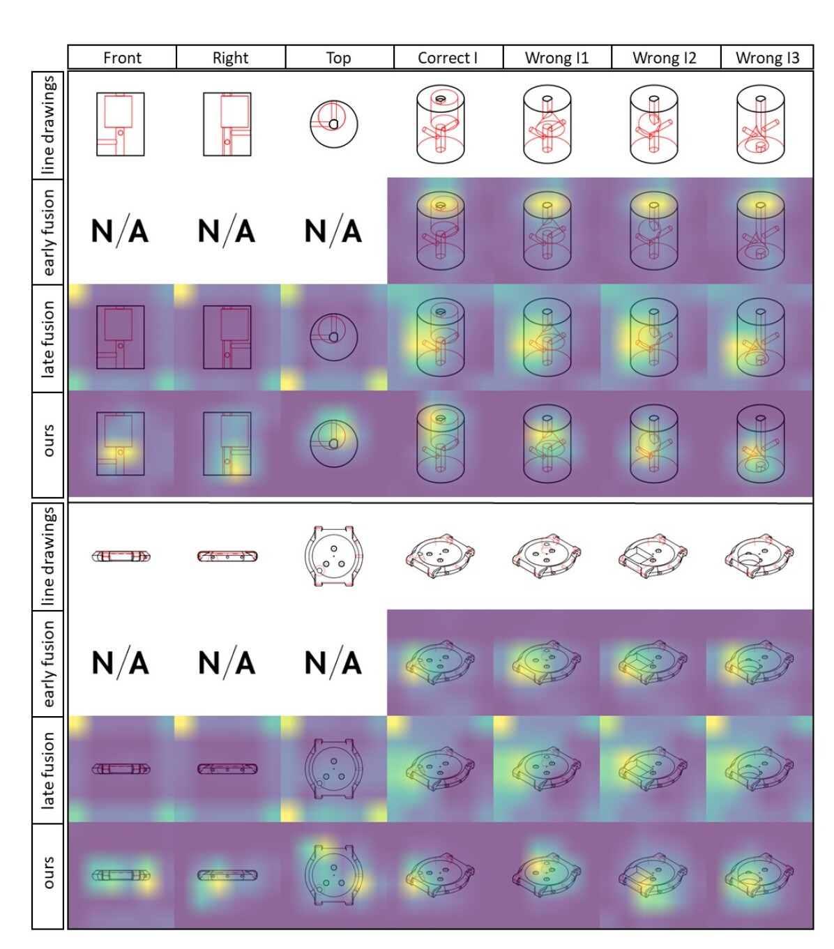
Figure 10: Attention maps for SL vs. SSL method in T2I task.

Appendix C Additional Attention Maps for T2I

We provide more visualization results of attention maps to compare our method with supervised learning method, as in Figure 10.