Topological Filtering for 3D Microstructure Segmentation

Abstract

Tomography is a widely used tool for analyzing microstructures in three dimensions (3D). The analysis, however, faces difficulty because the constituent materials produce similar grey-scale values. Sometimes, this prompts the image segmentation process to assign a pixel/voxel to the wrong phase (active material or pore). Consequently, errors are introduced in the microstructure characteristics calculation. In this work, we develop a filtering algorithm called PerSplat based on topological persistence (a technique used in topological data analysis) to improve segmentation quality. One problem faced when evaluating filtering algorithms is that real image data in general are not equipped with the ‘ground truth’ for the microstructure characteristics. For this study, we construct synthetic images for which the ground-truth values are known. On the synthetic images, we compare the pore tortuosity and Minkowski functionals (volume and surface area) computed with our PerSplat filter and other methods such as total variation (TV) and non-local means (NL-means). Moreover, on a real 3D image, we visually compare the segmentation results provided by our filter against TV and NL-means. The experimental results indicate that PerSplat provides a significant improvement in segmentation quality.

Keywords: Tomography, Topological persistence, Image segmentation, Image filtering, Tortuosity

1 Introduction

Microstructures are the building blocks of a material: the shape, size, interconnection, and orientation of these microstructures play a key role in defining the ultimate properties and performance. For example, in energy storage systems like lithium ion batteries (LIB), these microstructures influence the ability to store energy, the conversion rates, and the diffusion phenomena [1, 2, 3, 4, 5, 6, 7]. Hence, analyzing and visualizing these microstructures help us understand the properties of the materials and design new materials [8].

Nowadays, microstructures are frequently examined in 3D using X-ray computed tomography (XCT or CT) [9]. In XCT, X-ray images are collected from many different directions and are interpreted to yield 3D maps of local X-ray absorption strength quantified by a grey-scale [10]. Besides an extensive usage of XCT in materials science to characterize fuel cell electrodes [11, 12], super-capacitor electrodes [13], porous ceramics [14], and fiber orientation in composites [15], XCT is also used in biological applications such as tumor detection [16, 17], fracture examination [18, 19], and blood clots [20]. In battery research, the XCT experiments are performed to measure three important microstructure characteristics, i.e., the porosity, the specific surface area, and the tortuosity of pore network [1, 21, 22].

For the present work, we emphasize microstructural tortuosity as it directly influences current flow rates within the interpenetrating electrolyte phase contained in the pores. Typically, before calculating porosity or tortuosity, the data gathered from XCT are processed to assign each voxel/pixel to the solid phase or the pore phase; this process is called image segmentation (which means binarization for datasets of this paper). However, depending on the mixture of phases being studied and their ability to absorb X-rays, a ‘faithful’ binarization of data can be very difficult. Hence, an appropriate filtering before the binarization is often necessary to improve the quality of binarization and thereby the accuracy of computed microstructure characteristics [23, 24].

To illustrate the difficulty faced by a binarization algorithm without a proper filtering, we take the popular global thresholding algorithm Otsu [25] as an example. In Otsu, a threshold value is picked first, and then any pixel/voxel above (resp. below) the threshold value is assigned active material (resp. porous region). It is known that Otsu works well for images with bimodal histograms, where peaks of the two classes in the histograms are distinct. However, due to its strong reliance on histograms, Otsu algorithm may have difficulty when the peaks overlap and are not distinguishable. For example, Figure 1a shows a 3D grey-scale image with a bimodal histogram, and the binarization by Otsu preserves almost all important regions. In contrast, Figure 1b shows a 3D image whose histogram is not bimodal, and therefore the binarization by Otsu does not reflect the true porosity or electrolyte channel. In addition to the problem described above, data collected from XCT also have artifacts, which can potentially clutter the grey-scale values of pixels/voxels [26, 27] and hence further hinder the binarization process.

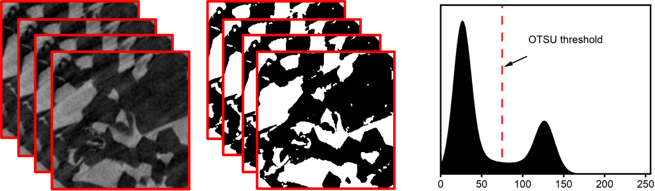
(a)

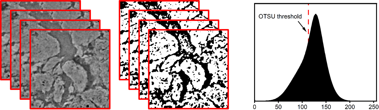
(b)

Figure 1: XCT data. (a) Grey-scale data, binarized data, and histogram of templated porous polymer. (b) Grey-scale data, binarized data, and histogram of commercial electrode.

Contribution.

The motivation of this work is to improve the binarization results of images with a new topological filter. Specifically, we propose a filtering algorithm called PerSplat based on techniques developed from topological data analysis [28, 29] (TDA). This algorithm exploits topological structures hidden in the data to filter out noise/speckle so that overlaps in the histogram can be reduced. The filtered data fed to a binarization algorithm afterwards can then have a better binarization result. Compared to traditional filtering algorithms (such as those described in [30, 31]), PerSplat algorithm has the following advantages:

1. Based on the theory of topological persistence [32], PerSplat detects global structures rather than local ones in a multi-scale manner. The removed noise can be of any shape which do not need to fit in a rectangular window. This is in contrast to traditional despeckling filtering algorithms [31] utilizing a moving window, which restricts the shapes of detected speckle.

2. In contrast to traditional despeckling or denoising algorithms [30, 31], which aim at recovering the ground-truth image, our algorithm aims at a filtering of the image so that the ensuing binarization can recover the true segmentation of the phases. Achieving such a goal is especially valuable when the ground truth image itself is hard to binarize. As indicated by experiments, the binarization by a standard scheme (such as Otsu) is more reliable with PerSplat.

3. Some small but significant features can be preserved by inhibiting the removal of those small regions that persist for a long range of values. This is achieved with the help of the well-established tool called barcodes [29, 32] (or persistence diagrams), in which long bars are considered as significant features and short bars are treated as noise.

We briefly describe our PerSplat algorithm in Section 2. In our experiments, PerSplat outperforms other general-purpose filtering methods (TV [33, 34] and NL-means [30]) on both synthetically generated datasets and natural datasets; see Section 3 for details.

1.1 Related works

Considering the volume of existing literature on the topic, we only briefly describe a few image filtering/denoising algorithms of various types. For a more comprehensive overview, we recommend the work by Buades el al. [30] on denoising for general images, the work by Loizou and Pattichis [31] on despeckling for ultrasound images, and the work by Kaestner et al. [24] on image filtering in porous media research. In our overview, we only describe the algorithms in 2D; their generalization to 3D is straightforward. Throughout, let $\Omega$ denote the domain of the image which is a rectangular region in $\mathbb{R}^{2}$, and an image is therefore treated as a function $v:\Omega\to\mathbb{R}$.

Total variation.

Total variation (TV) denoising [33, 34] draws upon a measurement of regularization $TV_{\Omega}(u)$ for an image $u$, which is the integral of the gradient magnitude. Given an input image $v$, TV denoising minimizes $TV_{\Omega}(u)$ for the denoised image $u$ subject to the following constraints:

$$\int_{\Omega}(u(x)-v(x))\mathrm{d}x=0\quad\text{and}\quad\int_{\Omega}|u(x)-v(x)|^{2}\mathrm{d}x=\sigma^{2}.$$

Alternatively, TV denoising solves a corresponding unconstrained minimization problem:

$$\arg\min_{u}TV_{\Omega}(u)+\lambda\int_{\Omega}|u(x)-v(x)|^{2}\mathrm{d}x,$$

where $\lambda$ is a weight parameter balancing the degree of the denoising and the fidelity to the input. In terms of denoising quality, TV denoising outperforms those simple methods (such as the median filtering) by preserving edges while reducing noise in flat areas.

Wavelet thresholding.

Wavelet thresholding filters work on the frequency domain. Let images now be defined on the discrete 2D grid $I$ instead of the continuous $\Omega$, and let $\mathcal{B}=\{g_{\alpha}\}_{\alpha\in A}$ be an orthonormal basis for $\mathbb{R}^{|I|}$. The input image $v:I\to\mathbb{R}$ can be decomposed into the form $v=\sum_{\alpha\in A}v_{\mathcal{B}}(\alpha)g_{\alpha}$, where each coefficient $v_{\mathcal{B}}(\alpha)$ is the scalar product $\langle v,g_{\alpha}\rangle$. Then, each coefficient $v_{\mathcal{B}}(\alpha)$ is modified to $a(\alpha)v_{\mathcal{B}}(\alpha)$, where $a(\alpha)$ is a value depending on $v_{\mathcal{B}}(\alpha)$. Wavelet thresholding recovers a denoised image as $u=\sum_{\alpha\in A}a(\alpha)v_{\mathcal{B}}(\alpha)g_{\alpha}$, and different wavelet thresholding filters differ on how $a(\alpha)$ is chosen for each $v_{\mathcal{B}}(\alpha)$. Specifically, soft wavelet thresholding [35] sets $a(\alpha)$ as:

$$a(\alpha)=\begin{cases}\;\frac{v_{\mathcal{B}}(\alpha)-\text{sgn}(v_{\mathcal{B}}(\alpha))\mu}{v_{\mathcal{B}}(\alpha)},&|v_{\mathcal{B}}(\alpha)|>\mu,\\ \;0,&\text{otherwise,}\end{cases}$$

where $\mu$ is a threshold parameter. Translation invariant wavelet thresholding [36] further improves soft wavelet thresholding by averaging the denoising results on all translations of the input image, which could reduce the so-called Gibbs effect.

NL-means.

The name NL-means [30] is short for ‘non-local’ means which comes from its difference to those ‘local mean’ filters. Given an input image $v$, NL-means produces the following denoised pixel $u(x)$ for a given position $x\in\Omega$:

$$u(x)=\frac{1}{C(x)}\int_{\Omega}e^{-\frac{L_{a}(x,y)}{h^{2}}}v(y)\mathrm{d}y,$$

in which $h$ is a filtering parameter, $C(x)$ is a normalizing factor, and $L_{a}$ is a measure of dissimilarity of the Gaussian neighborhood of two pixels. Specifically, let $G_{a}$ be a Gaussian kernel with standard deviation $a$, we have

$$L_{a}(x,y)=\int_{\mathbb{R}^{2}}G_{a}(t)|v(x+t)-v(y+t)|^{2}\mathrm{d}t.$$

Hence, $u(x)$ is the mean of the other pixels whose Gaussian neighborhood is similar to $x$. NL-means produces denoised images with greater clarity and less detail loss compared to those local mean algorithms.

UINTA.

UINTA [37] stands for ‘unsupervised, information-theoretic, adaptive filter’. For each pixel $x$ and its neighborhood $N_{x}$, UINTA uses stochastic gradient descent to reduce the entropy (expectation of negative log-probability) of the conditional probability density $P(X=x\,|\,N_{X}=N_{x})$, where $P(X=x\,|\,N_{X}=N_{x})$ is estimated by the Parzen-window non-parametric density estimation technique [38] with an $n$-dimensional Gaussian kernel. The design of UINTA is based on the observation that adding noise to the original signal greatly increases the entropy. Hence, decreasing the entropy mitigates randomness in the observed PDF’s and so noise can be reduced. Note that UINTA resembles NL-means in a sense that it also involves comparing the neighborhood of pixels for computing a denoised value.

2 PerSplat algorithm

We only describe the PerSplat algorithm in 2D; its 3D version follows similar steps. There are two stages in the algorithm, and since the second stage is a reversal of the first stage, we only briefly overview the first stage before presenting the details. In the first stage, we traverse the grey-scale values of the input image in increasing order starting from zero. For each value $s$ traversed, we consider pixels in the image with grey-scale values no greater than $s$ (i.e., the sublevel set) and take the connected components of these pixels. As $s$ increases, we track the following changes of connected components in the sublevel sets:

1. A new connected component which does not correspond to any previous ones is created; this happens at a local minimum in the image.

2. Connected components grow larger.

3. Several connected components merge into the same component.

Consider a merging that happens, say at a grey-scale value $s$. We ‘splat’ any connected component $\mathsf{C}$ that is getting merged with size and persistence length (defined later) no greater than some input parameters. By splatting a component, we mean to assign the grey-scale value $s$ to all its pixels. Intuitively, the splatting suppresses those small ‘downward’ (dark) bumps, which serves as a noise reduction for the image. Symmetrically, splatting in the second stage suppresses those small ‘upward’ (bright) bumps; see the discussion and figure presented later in the section for more details.

Full details.

We formalize a 2D input image as a function $f:\mathsf{G}\to[0,M]$, where $[0,M]$ is an interval of integers with $M$ usually equal to 255. Moreover, $\mathsf{G}$ is the graph corresponding to the 2-dimensional grid of an image, i.e., vertices of $\mathsf{G}$ correspond to pixels in the image and connect to either 4 or 8 of its neighbors. We also have that function values of $f$ on the vertices are grey-scale values of the corresponding pixels.

For any $s\in[0,M]$, define $f_{s}$ as the full subgraph of $\mathsf{G}$ containing vertices whose function values are no greater than $s$. We have that $f_{s}$ is a subgraph of $f_{t}$ whenever $s\leq t$. Therefore, starting from $s=0$, $f_{s}$ keeps growing larger as $s$ increases and eventually equals the entire $\mathsf{G}$. For an $s$, we consider the connected components of $f_{s}$, i.e., those maximal sets of vertices of $\mathsf{G}$ in which each pair admits a connecting path. As we increase the value of $s$, the following three types of events can happen, in which we pay attention to the first and the third one (i.e., the critical events):

1. A new connected component in $f_{s}$ which has no correspondence in $f_{s-1}$ is created.

2. Connected components of $f_{s-1}$ grow larger in $f_{s}$.

3. Several connected components of $f_{s-1}$ merge into the same connected component in $f_{s}$.

The algorithm requires two parameters $\mu$ and $\lambda$ as inputs, where $\mu$ denotes the maximum speckle size and $\lambda$ denotes the maximum persistence length of a connected component that the algorithm can modify. Note that we always set $\lambda=\infty$ in experiments so that the algorithm can modify any connected component.

The algorithm contains two stages, where the first stage increasingly enumerates $s$ from $0$ to $M$. During the first stage, whenever a merging happens at $s$, for each connected component $\mathsf{C}$ of $f_{s-1}$ that merges with others, we define the following:

• Let $|\mathsf{C}|$ denote the size of $\mathsf{C}$, which is the number of vertices of $\mathsf{C}$.

• Let $\text{b}(\mathsf{C})$ denote the birth value of $\mathsf{C}$, which is the least function value of $\mathsf{C}$’s vertices.

• Let $\ell(\mathsf{C})$ denote the persistence length of $\mathsf{C}$, which is defined as $\ell(\mathsf{C})=|s-\text{b}(\mathsf{C})|$.

If $|\mathsf{C}|$ is no greater than $\mu$ and $\ell(\mathsf{C})$ is no greater than $\lambda$, we assign the value $s$ to all pixels corresponding to the vertices of $\mathsf{C}$, i.e., the connected component $\mathsf{C}$ is splatted to value $s$ (see Figure 2). Note that the creation and merging of connected components actually construct the merge tree of $f$, which is a well-known tool in topological data analysis (TDA).

The second stage is a reverse process of the first: the value $s$ is enumerated decreasingly from $M$ to 0. Since the input image has been modified in the first stage, we let $g:\mathsf{G}\to[0,M]$ denote the function corresponding to this modified image. Furthermore, we define $g^{s}$ as the full subgraph of $\mathsf{G}$ containing vertices whose function values (on $g$) are no less than $s$. Therefore, as $s$ decreases, connected components in $g^{s}$ can also get created, grow, or merge with others. Note that birth value in this case is the greatest function value of the connected component. We then modify the pixel values for a connected component whenever a merging happens, which is similar to the previous stage.

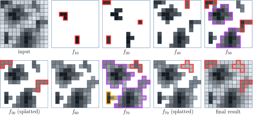
Figure 2: An exemplar run of the first stage of PerSplat. As $s$ increases, connected components can be created (e.g., red ones in $f_{10}$) or grow larger. The connected components can also merge among which some get splatted (e.g., red ones in $f_{50}$) while some are preserved (e.g., purple and orange ones in $f_{70}$).

As mentioned earlier, the first stage suppresses those small ‘downward’ bumps for the image and the second stage suppresses those small ‘upward’ bumps. The parameters $\mu$ and $\lambda$ control how aggressive the suppressing is, in which trade-offs need to be made between noise filtering and possible loss of details. Figure 2 illustrates an exemplar run ($\mu=5$, $\lambda=30$) of the first stage, where the input image is considered to have six dark spots. Three smaller, less dark spots are splatted (i.e., turn to grey; see the red squares in the final result), leaving the remaining three spots which are more prominent preserved. In the exemplar run, $f_{10}$ creates two connected components, while $f_{20}$ and $f_{40}$ create three and one component(s) respectively; the newly created components are marked by red squares. Note that these connected components are constantly growing after being created. In $f_{50}$, two pairs of connected components merge together in which the ones marked by red squares are splatted because of their sizes and persistence lengths. In $f_{70}$, all four connected components are merged where the one inside the red square is splatted; note that though the connected component inside the orange square has a size no greater than $\mu$, it is not splatted due to a longer persistence length than $\lambda$.

Finally, we observe the following property of PerSplat, which confirms the consistency of choices made to modify a connected component:

For any node on the merge tree which is splatted by the algorithm, all its descendants are splatted. Equivalently, for any node which is not splatted, all its ancestors are not.

3 Results and discussion

In this section, we demonstrate the efficacy of our PerSplat algorithm by comparing it with two general-purpose filtering algorithms: TV [33, 34] and NL-means [30]. After applying the filters, we use the global thresholding algorithm Otsu [25] as a benchmark for binarization. Note that although some other types of binarization algorithms (such as locally adaptive thresholding [23]) may produce better results in some cases, we choose Otsu because of its simplicity and effectiveness [23]. Since the focus of the paper is on image filtering for XCT data, using Otsu is sufficient for our purposes.

We briefly summarize our experiments as follows:

1. Using Otsu for binarization, we compare the tortuosity computed from PerSplat, TV, and NL-means filtering to the ground-truth tortuosity for some synthetically generated images; see Section 3.1 for details.

2. We apply PerSplat, TV, and NL-means for filtering a natural 3D image and visually compare the binarization results by Otsu; see Section 3.2 for details.

Note that we apply our PerSplat algorithm on 3D grey-scale images in two ways in this paper:

PerSplat-P (i.e., PerSplat-Pixelized):

In this case, we process the 3D image slice by slice using the version of PerSplat for 2D input. The outputs for all slices are then stacked to create a 3D filtered image.

PerSplat-V (i.e., PerSplat-Voxelized):

In this case, all slices together are processed by the version of PerSplat for 3D input.

3.1 Results on synthetic datasets

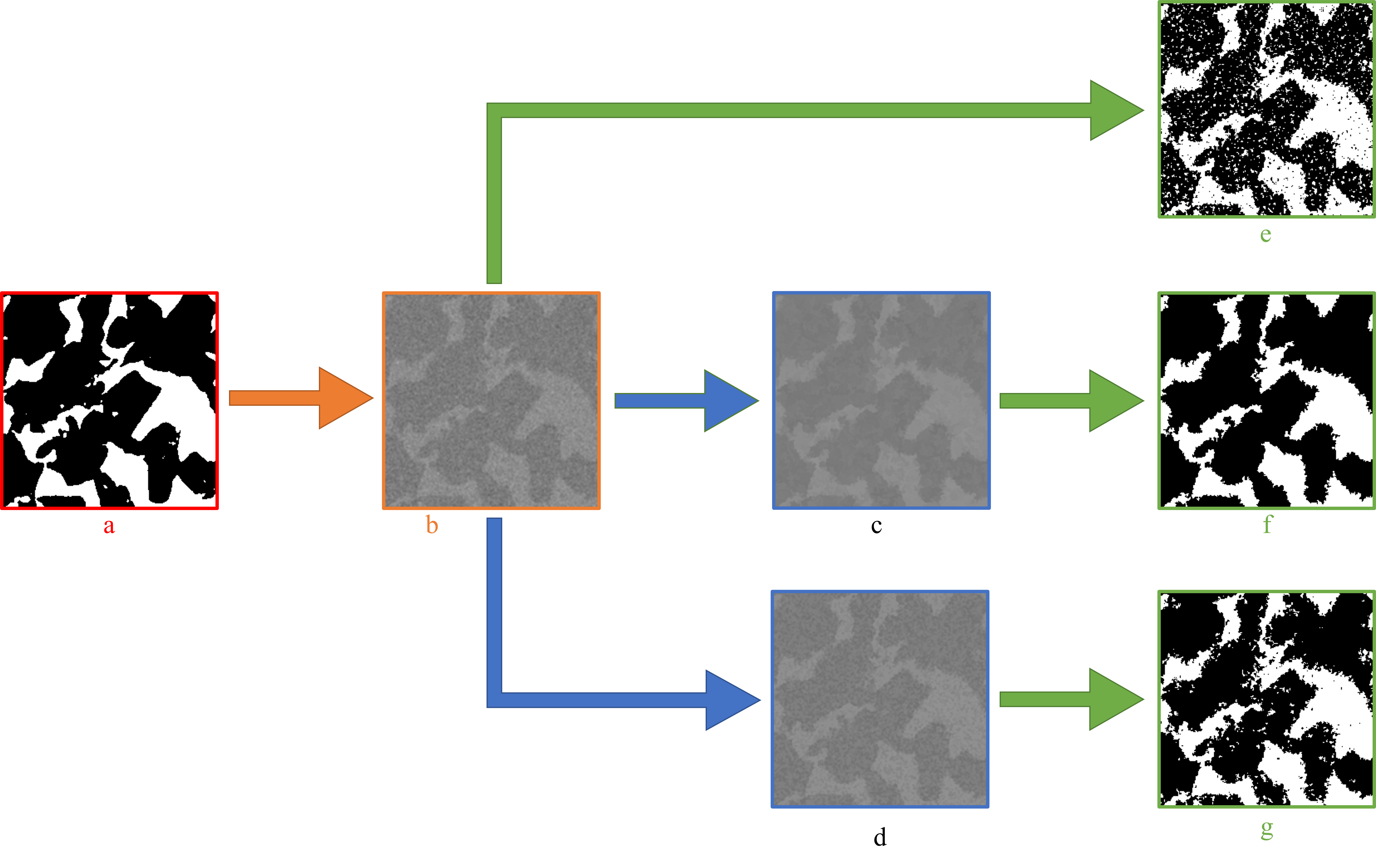
Figure 3: Processing pipeline on synthetic datasets. (a) A ground-truth slice of Synth1. (b) Slice with synthetic noise added. (c) Noisy slice filtered by PerSplat-P. (d) Noisy slice filtered by PerSplat-V. (e,f,g) Binarized slices by Otsu.

The absence of ground truth for the XCT data [39] makes it hard to evaluate the segmentation quality. Hence, to address the issue of ‘missing’ ground truth, we create synthetic images whose ground-truth values are known, with the following process:

1. Given a 3D XCT image, we first binarize the image with Otsu and take this binarized image as ground truth, i.e., we take voxels with values greater than the threshold as in the solid phase and the rest as in the porous phase.

2. We then introduce noise to the established ground-truth image based on Gaussian distribution (see Section 4 for further details). The introduction of Gaussian noise is justified by the fact that nearly all images we obtain through XCT have histograms akin to a mixture of Gaussians as shown in Figure 1.

3. We also apply noise to the image based on Poisson distribution. The rationale behind the Poisson noise is as follows. Typically, noise in XCT images is caused by various factors such as the number of scans performed, the object being measured, and the data processing methodology employed. One such factor is called ‘shot noise’ or ‘quantum noise’, which is introduced because photons in the X-ray beam follow a spatial distribution according to the Poisson law [40].

4. Finally, for each voxel, we apply a nearest neighbor averaging in three dimensions to account for averaging of the XCT signal that happens at the interfaces.

In Figure 3, we show the processing pipeline on the synthetic datasets with PerSplat-P and PerSplat-V for filtering. After the binarization, we calculate the tortuosity for the binarized images using a MATLAB open-source application TauFactor [41].

Overall results.

Based on different ground truths, we generate synthetic datasets with different degrees of overlaps in the histograms. To control the histogram overlap, we adjust the mean and variance of the Gaussian noise for the two phases: when the mean for the two phases is close or the variance is large, overlap in the histogram is significant (see Section 4 for more details).

Table 1 provides details of the generated synthetic datasets, where we list the data sources (i.e., the data samples from which we derived our ground truth), black phase fractions of the ground-truth images, and the Gaussian noise parameters for the two phases. The ground truths for Synth1 and Synth2 are extracted from (different regions of) the XCT data of porous templated polymer. The ground truths for Synth3 and Synth4 are extracted from the tomographic data of a commercial LIB anode [1, 27]. The two sets of samples, porous polymer and LIB anode, are selected because of their difference in the phase fractions. Note that the histogram of Synth2 has more overlap than that of Synth1 as exhibited by Table 1; similar difference holds for Synth3 and Synth4.

Table 1: Statistical setting for generated synthetic data. The ground truths for Synth1 and Synth2 are extracted from porous polymer. The ground truths for Synth3 and Synth4 are extracted from LIB anode. Active material is assigned as white phase while porous region is assigned as black phase.

Dataset	Data source	Black phase fraction	White phase		Black phase
			Mean	Var	Mean	Var
Synth1	porous polymer	66%	100	25	85	25
Synth2	porous polymer	75%	87	35	80	35
Synth3	LIB anode	35%	100	25	85	25
Synth4	LIB anode	35%	87	35	80	35

Table 2: Microstructure characteristics and binarization accuracy computed. For each type of microstructure characteristics, we list the difference to the ground-truth value calculated from each filter. The best values are underlined.

Data	Methods	Tortuosity			Charac. Tor.	Pixel Accur.	White Vol.	White Surf. Area
		1	2	3
Synth1	Ground Truth	1.668	1.668	1.890	1.736	-	6058513	1.03E+06
	No Filtering	+0.272	+0.274	+0.274	+0.274	90.45%	+586589	+2.32E+06
	PerSplat-P	+0.037	+0.036	+0.138	+0.065	95.95%	+99754	+2.98E+05
	PerSplat-V	+0.146	+0.146	+0.192	+0.160	93.84%	+379728	+1.12E+06
	NL-means-2D	+0.272	+0.274	+0.274	+0.274	90.45%	+586492	+2.32E+06
	NL-means-3D	+0.271	+0.272	+0.273	+0.273	90.48%	+579665	+2.31E+06
	TV	$-$0.127	$-$0.130	$-$0.184	$-$0.144	93.70%	+79869	$-$3.03E+05
Synth2	Ground Truth	1.392	1.391	1.345	1.376	-	4213761	7.58E+05
	No Filtering	+1.239	+1.233	+1.203	$-$1.225	64.02%	+3878836	+6.96E+06
	PerSplat-P	+0.635	+0.646	+2.027	$-$0.966	72.74%	+3600816	+4.87E+06
	PerSplat-V	+1.427	+1.425	+1.665	$-$1.503	62.29%	+4527724	+6.74E+06
	NL-means-2D	+1.239	+1.233	+1.203	$-$1.225	64.02%	+3878766	+6.96E+06
	NL-means-3D	+1.202	+1.198	+1.172	$-$1.191	64.26%	+3811400	+6.96E+06
	TV	$-$0.064	$-$0.058	$-$0.033	+0.051	93.85%	+303944	$-$4.93E+04
Synth3	Ground Truth	3.078	2.701	3.496	3.058	-	5530602	1.73E+06
	No Filtering	+0.171	+0.244	$-$0.140	$-$0.116	82.75%	$-$568356	+9.78E+05
	PerSplat-P	+0.189	+0.063	+0.570	$-$0.225	86.22%	+76852	+2.26E+04
	PerSplat-V	+0.151	+0.202	$-$0.078	$-$0.111	84.01%	$-$399765	+7.32E+05
	NL-means-2D	+0.171	+0.245	$-$0.140	$-$0.116	82.76%	$-$568284	+9.78E+05
	NL-means-3D	+0.151	+0.232	$-$0.160	$-$0.099	82.65%	$-$583979	+9.90E+05
	TV	$-$0.803	$-$0.328	$-$1.443	+0.832	74.63%	+90793	$-$1.12E+06
Synth4	Ground Truth	3.078	2.701	3.496	3.058	-	5530602	1.73E+06
	No Filtering	$-$0.402	$-$0.080	$-$0.821	+0.400	62.90%	$-$1216905	+2.33E+06
	PerSplat-P	$-$0.365	$-$0.112	+2.609	$-$0.208	69.39%	$-$651080	+1.48E+06
	PerSplat-V	$-$0.296	+0.026	$-$0.335	+0.180	63.88%	$-$962743	+2.23E+06
	NL-means-2D	$-$0.403	$-$0.079	$-$0.820	+0.400	62.91%	$-$1216840	+2.33E+06
	NL-means-3D	$-$0.405	$-$0.077	$-$0.819	+0.400	62.90%	$-$1213542	+2.34E+06
	TV	$-$0.816	$-$0.555	$-$1.102	+0.795	71.82%	$-$439236	$-$8.00E+05

In Table 2, we show the following values computed with the different filters for each dataset in Table 1:

• tortuosity in the three directions and the characteristic tortuosity (the harmonic mean of tortuosity in the three directions);

• volume and surface area of the white phase, which are a subset of the Minkowski functionals [42];

• binarization accuracy, which is the percentage of voxels correctly classified.

We also underline the best values achieved in Table 2. Note that ‘NL-means-2D’ means that NL-means is applied independently to each slice and ‘NL-means-3D’ means that NL-means is applied to the entire stack at once. We fix the parameters of the filtering algorithms for all the datasets in Table 2:

• for PerSplat-P, we use a speckle size $\mu=54$;

• for PerSplat-V, we use a speckle size $\mu=500$;

• for TV, we use a regularization weight of 0.5;

• for NL-means-2D and -3D, we use the default parameters of the implementation provided by scikit-image [43].

From Table 2, we observe that PerSplat-P or PerSplat-V are consistently providing the most accurate tortuosity values. The only exception is Synth2, whose best values are provided by TV. However, on Synth2, the tortuosity values provided by PerSplat are still comparable to those provided by NL-means. As for the volume and surface area of the white phase shown in Table 2, we observe that TV provides the best results with PerSplat-P performing comparably well, whereas PerSplat-P and PerSplat-V consistently outperform NL-means.

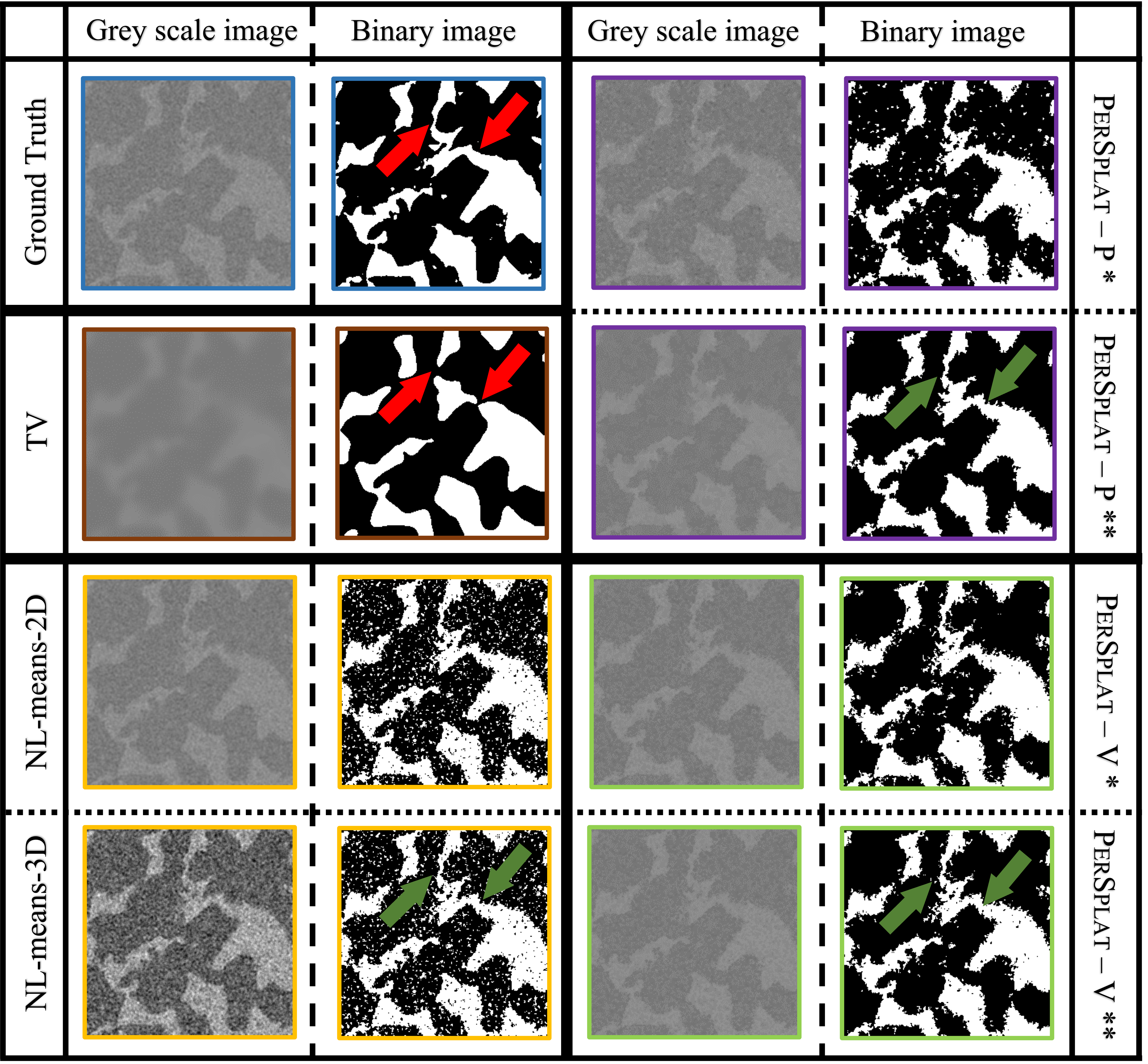
Figure 4: Grey-scale images filtered by all methods and their binarized version for one slice of Synth1, with the unfiltered slice and the ground-truth binarization also shown. Slices processed by different filters are marked with different colors. PerSplat-P^∗ has $\mu=10$; PerSplat-P^∗∗ has $\mu=54$; PerSplat-V^∗ has $\mu=500$; PerSplat-V^∗∗ has $\mu=14659$.

For one slice of Synth1, we show in Figure 4 the corresponding grey-scale images filtered by methods in Table 2 and the binarized version by Otsu; the original unfiltered slice of Synth1 and the ground-truth binarization are also shown. We also include in Figure 4 the results from PerSplat using two speckle sizes ($10\text{ and }14659$) different from the ones (54 and 500) used to generate Table 2. From the binarized image with TV filtering in Figure 4, we observe that the white connected component marked by the red arrows is inaccurately disconnected. To the contrary, PerSplat and NL-means both preserve the connected component as indicated by the green arrows in Figure 4. Also note that the binarized images with NL-means filtering in Figure 4 have many speckles which the ground truth does not have. In contrast, the speckles are largely avoided by PerSplat (especially PerSplat-P with speckle size 54).

Varying speckle size.

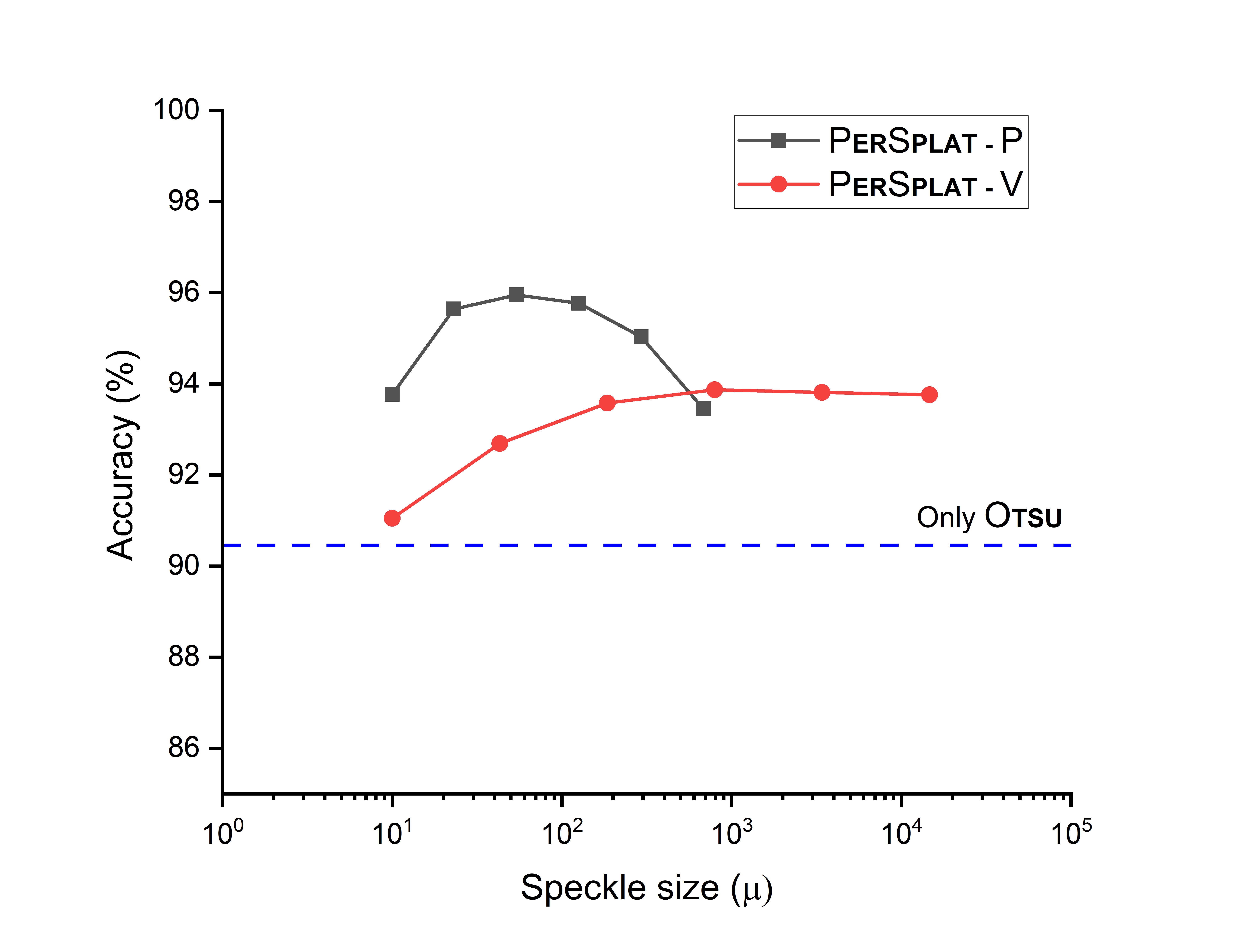
(a)

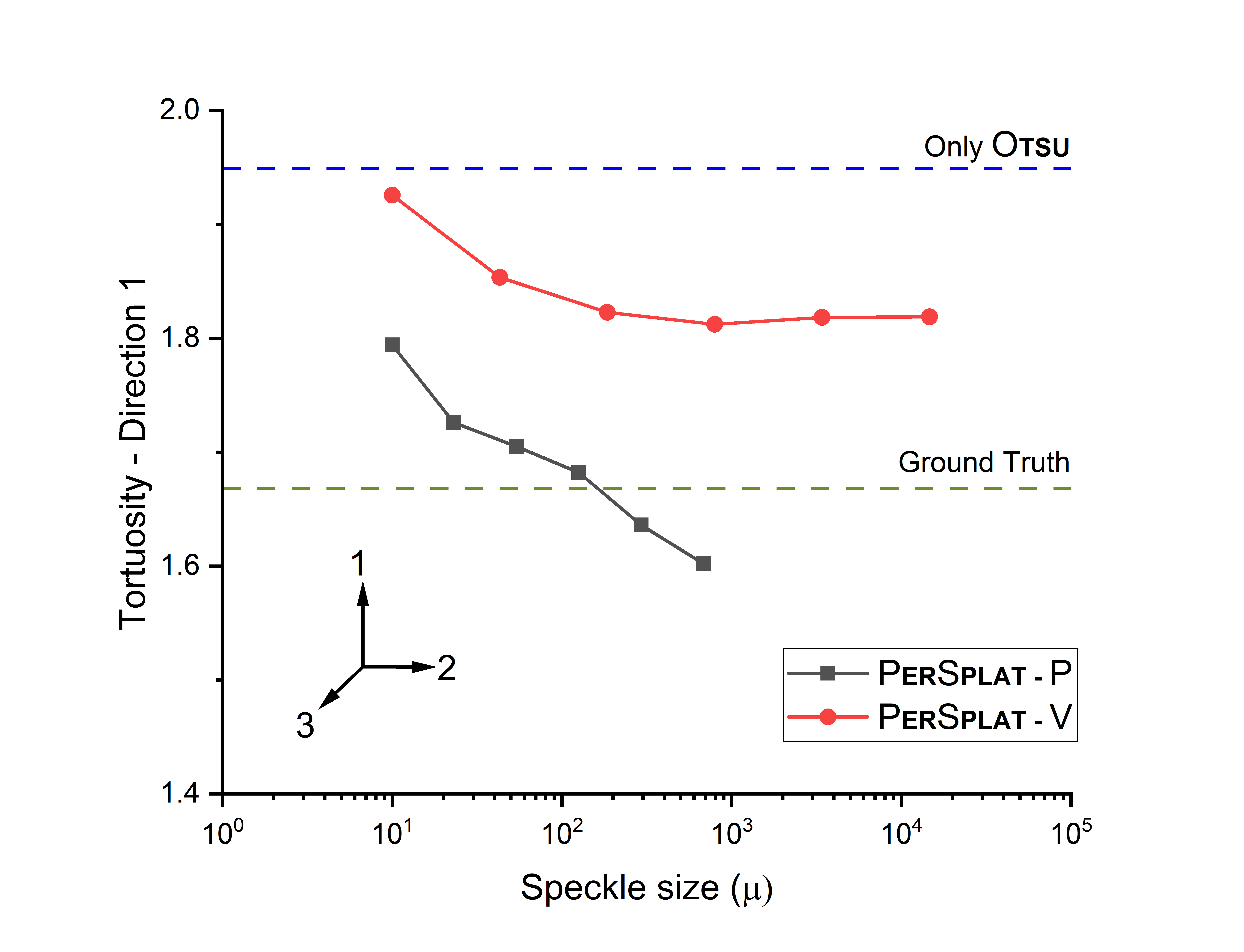
(b)

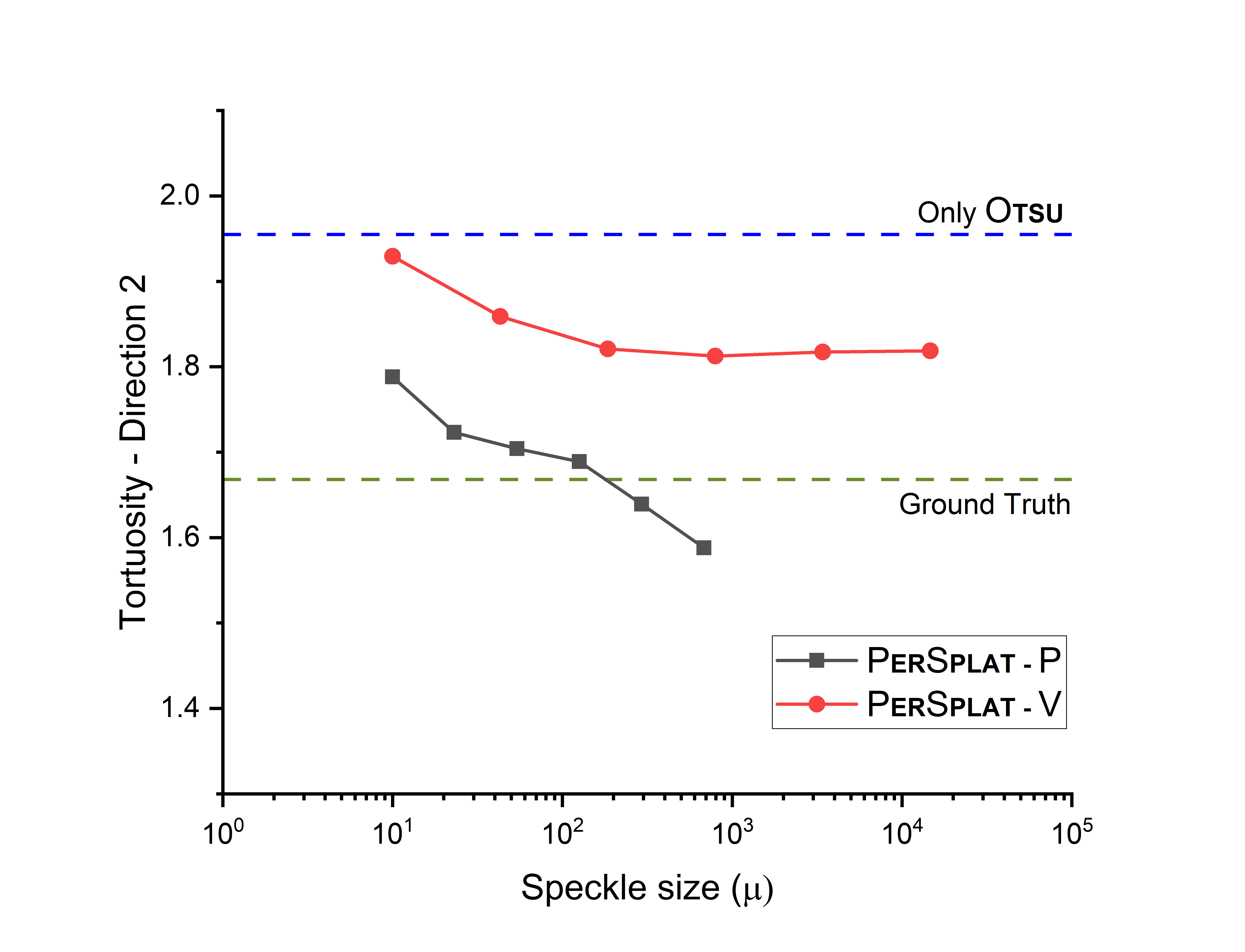
(c)

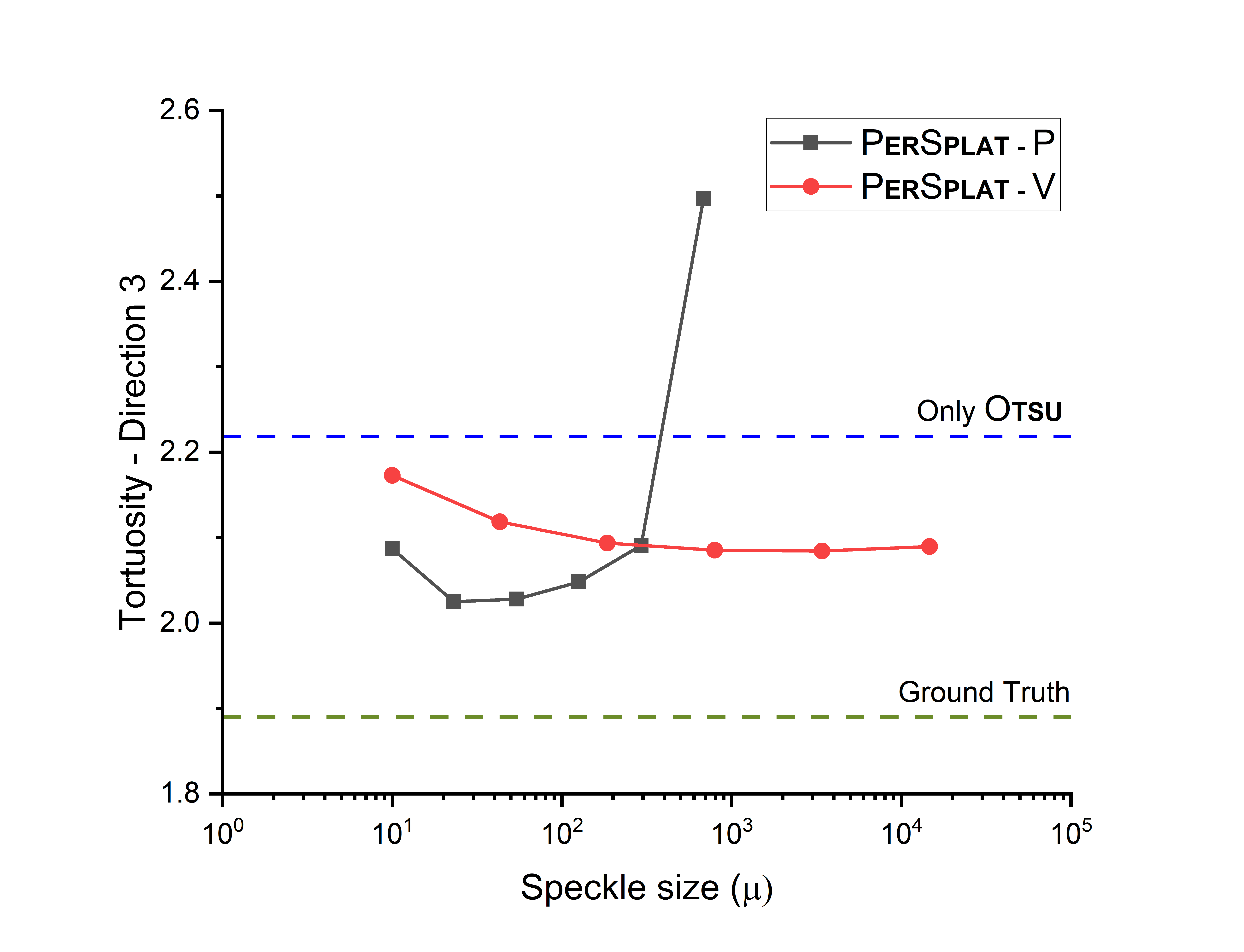
(d)

Figure 5: Microstructure analysis with various speckle size ($\mu$) parameters for PerSplat. The input dataset is Synth1 and horizontal axes for the $\mu$ parameter are re-scaled by logarithm function. (a) Binarization accuracy as a function of $\mu$. (b-d) Tortuosity as a function of $\mu$ in the three directions.

Recall that, with PerSplat, the user needs to choose a speckle size parameter $\mu$ as input. To provide guidance on the parameter choosing, in Figure 5, we show how various $\mu$ parameters impact the binarization accuracy and the computed tortuosity. The input dataset for Figure 5 is Synth1 and the speckle sizes exponentially range from 10 to 682 for PerSplat-P, from 10 to 14659 for PerSplat-V. From Figure 5, we observe that the change of speckle size has a more significant effect on tortuosity when using PerSplat-P, while tortuosity appears to be more stable at various speckle sizes when using PerSplat-V. This is a result of the additional dimension of connectivity introduced in 3D. To understand the phenomenon, imagine running PerSplat on 2D and 3D images: as the value $s$ increases/decreases (see the description of the algorithm), the sizes of the connected components grow much faster in 3D than in 2D because of the additional dimension of connectivity. In 3D, the connected components quickly grow very large; to splat them, we need a large $\mu$ parameter. This makes nearly the same components to be splatted for a wide range of $\mu$ when running PerSplat on 3D images (PerSplat-V).

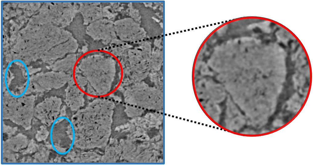
(a)

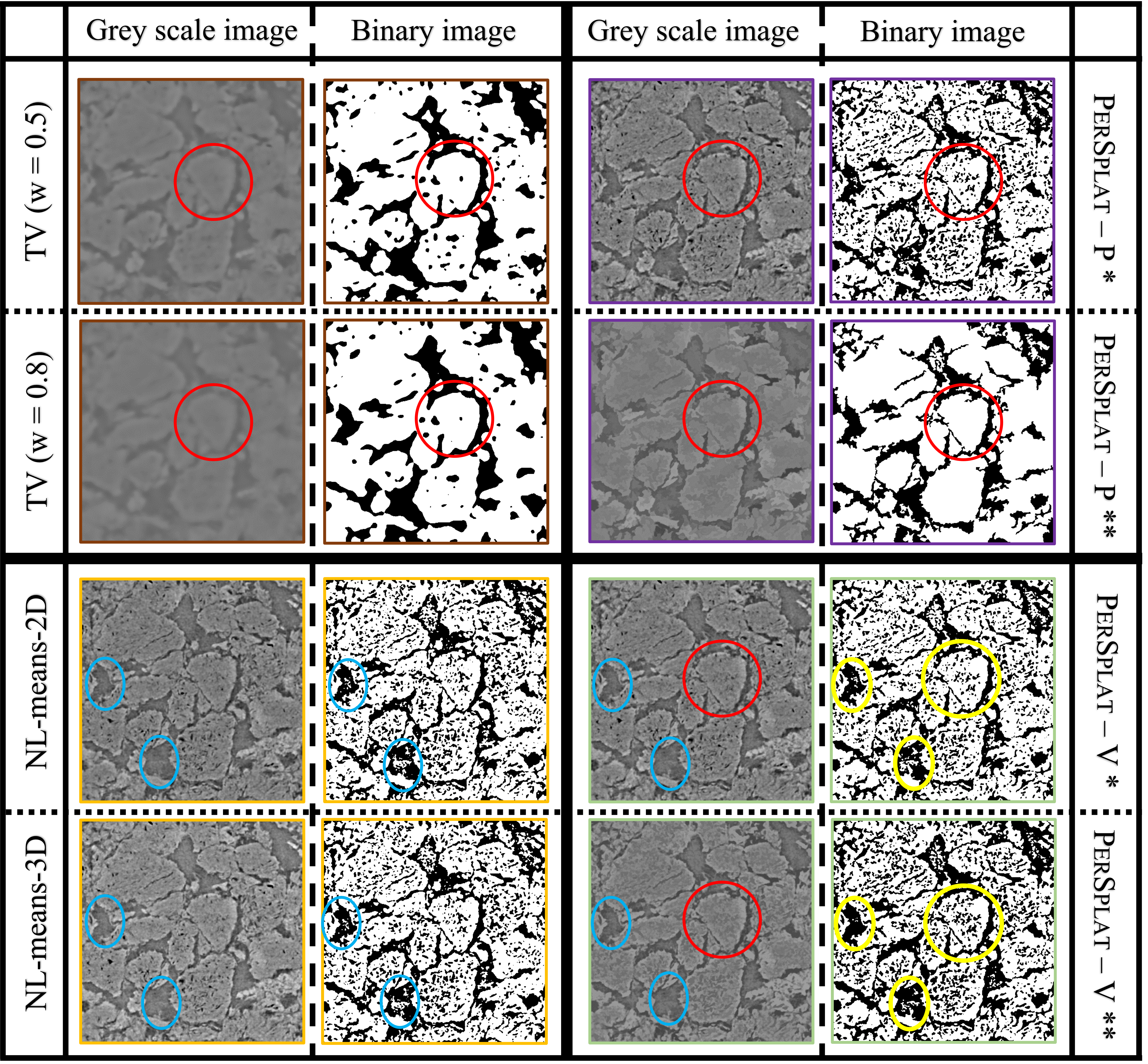
(b)

Figure 6: One slice of a natural XCT dataset processed by different filters. (a) The input unfiltered slice. (b) Filtered and binarized slices, with the slices processed by different filters marked with different colors. PerSplat-P^∗ has $\mu$ = $10$; PerSplat-P^∗∗ has $\mu$ = $293$; PerSplat-V^∗ has $\mu$ = $10$; PerSplat-V^∗∗ has $\mu$ = $14659$.

3.2 Results on natural datasets

In Figure 6, we show the filtered images by the three methods (TV, NL-means, PerSplat) and their Otsu-binarized results for one slice of a natural XCT dataset. The natural XCT dataset is gathered from a tomography experiment from an open source [26]. By visually examining the results in Figure 6, we notice that TV produces overly smoothed images in which many important details (e.g., ones inside the white phase marked by the red circle) are lost. In contrast, NL-means (2D and 3D) manage to preserve most of the important details inside the white phase marked by the red circle. However, with NL-means filtering, some other important regions are not correctly binarized. For example, the two regions marked by the blue circles almost completely fall in the black phase; but in the binarized slices filtered by NL-means, a significant proportion of the two regions is still white. We then conclude that PerSplat filtering (e.g., PerSplat-V with $\mu=14659$) provides the best binarized slices visually. On one hand, the important details inside the white phase marked by the red circle are preserved; on the other hand, a larger proportion is classified as black in the two regions marked by the blue circles.

4 Methods

Software used.

MATLAB (R2019) was used to generate synthetic images, calculate binarization accuracy, and calculate tortuosity. ImageJ [44] was used for an implementation of Otsu. The Python library scikit-image [43] was used for implementations of TV and NL-means.

XCT Data used.

One of the microstructures used in this study is a porous polymer, Polydimethylsiloxane (PDMS). This sample was made by AVP in DPB’s lab using the process of templating where sugar cubes (Domino brand) were used as a template. The second sample is raw tomographic data obtained from [26] which is open-source. We performed X-ray Computed Tomography (XCT) on the porous PDMS. The sample in the open-source tomographic data is of commercially available lithium-ion batteries graphite electrode [27].

Adding synthetic noise.

To add noise to a given ground-truth image in the process of synthetic data generation, we took three steps. In step one, for each voxel from the black phase, we assign the voxel a grey-scale value based on a Gaussian distribution (for the black phase) of selected mean and variance. For voxels from the white phase, we perform similar operations. In step two, we used MATLAB’s in-build function ‘imnoise’ to create Poisson noise. This MATLAB function’s output depends on the type of input image (eg. 8 bit or 16 bit; our input was a 8 bit image). As the last step, we do a simple nearest neighbor averaging of the grey-scale values. This pays attention to near-neighbor voxel value averaging that often happens at boundaries between two phases in real XCT deconvolutions – as evidenced by the broad and flat region between the two Gaussians (see Figure 1a).

X-ray tomography.

XCT images for porous polymer (PDMS) were produced using X-ray nano-computed tomography. Computed tomography is a non-destructive technique that allows full 3D spatial density maps of an object. To gather these tomographic images, two major steps were taken. First, the sample was inserted inside a CT machine called ‘SkyScan1272’ manufactured by Bruker (Billerica, MA). A Hamamatsu L10101 micro-focus X-ray source was used with no filter. The X-ray source voltage and current was set to 40 kV and 200 $\mu\text{A}$, respectively, to get the best scan resolution. After setting up the X-ray source, a flat field correction was updated to minimize ring artifacts. A total scan of the sample contained 1472 projection images with a length and width of 2036 pixels by 2036 pixels, respectively. Images were taken at different angles equally spaced at 0.2^∘ on a scale of 0^∘ to 180^∘, with exposure time of 225 ms and frame averaging of 5 per rotation. Secondly, to get 3D volume data, reconstruction of the above acquired raw data was done using a program called NRecon (Version: 1.7.4.6). The final resolution of each image was 4.50 $\mu\text{m}$/pixel.

5 Conclusion

The investigation in this paper starts with an examination of the grey-scale histograms of commercial lithium-ion battery and a porous PDMS templated material. From the binarization results, we find that some important features of the microstructure are misinterpreted due to the histogram overlap, which led to miscalculation of microstructure characteristics. To solve the problem, we design a novel filtering algorithm called PerSplat based on topological persistence to rectify the small regions that are assigned to wrong group otherwise during binarization (specifically by Otsu). A tortuosity analysis and Minkowski functional calculations (volume and surface area) show that the ground-truth values are better approximated when the data is preprocessed with PerSplat and then binarized, as compared to a direct binarization. Also, PerSplat outperforms other filtering algorithms such as TV and NL-means in most cases. The PerSplat algorithm has two variations when being applied on 3D data: PerSplat-P and PerSplat-V. From our analysis, we observe that PerSplat-V has more stability over various speckle sizes. We hope that this algorithm, in general, can make the microstructure characteristics computations more reliable and hence help design better electrochemical devices. Additionally, the use of this algorithm is not only limited to battery research but potentially also to other applications engaging image analysis, ranging from tumor detection in biological sciences to detecting water content in geology.

References

- [1] P. Pietsch, M. Ebner, F. Marone, M. Stampanonibc, and V. Wood. Determining the uncertainty in microstructural parameters extracted from tomographic data. Sustainable Energy Fuels, 2(3):598–605, 2018.
- [2] J. M. Tarascon and M Armand. Issues and challenges facing rechargeable lithium batteries. In Materials for Sustainable Energy: A Collection of Peer-Reviewed Research and Review Articles from Nature Publishing Group, pages 171–179. 2010.
- [3] Shunsuke Yamakawa, Shingo Ohta, and Tetsuro Kobayashi. Effect of positive electrode microstructure in all-solid-state lithium-ion battery on high-rate discharge capability. Solid State Ionics, 344:115079, jan 2020.
- [4] Chien-Fan Chen, Ankit Verma, and Partha P. Mukherjee. Probing the Role of Electrode Microstructure in the Lithium-Ion Battery Thermal Behavior. Journal of The Electrochemical Society, 164(11):E3146–E3158, may 2017.
- [5] Bereket Tsegai Habte and Fangming Jiang. Effect of microstructure morphology on Li-ion battery graphite anode performance: Electrochemical impedance spectroscopy modeling and analysis. Solid State Ionics, 314:81–91, jan 2018.
- [6] Juan Alfonso Campos, Abhas Deva, Jarrod Lund, Aniruddha Jana, Ilenia Battiato, and R. Edwin García. Porous Electrode Phase Transition Kinetics in Li-Ion Batteries. ECS Meeting Abstracts, MA2020-01(1):83–83, may 2020.
- [7] L. Gireaud, S. Grugeon, S. Laruelle, B. Yrieix, and J. M. Tarascon. Lithium metal stripping/plating mechanisms studies: A metallurgical approach. Electrochemistry Communications, 8(10):1639–1649, oct 2006.
- [8] Xuekun Lu, Antonio Bertei, Donal P Finegan, Chun Tan, Sohrab R Daemi, Julia S Weaving, Kieran B. O’Regan, Thomas M.M. Heenan, Gareth Hinds, Emma Kendrick, Dan J.L. Brett, and Paul R Shearing. 3D microstructure design of lithium-ion battery electrodes assisted by X-ray nano-computed tomography and modelling. Nature Communications, 11(1), 2020.
- [9] Oluwadamilola O. Taiwo, Melanie Loveridge, Shane D. Beattie, Donal P. Finegan, Rohit Bhagat, Daniel J.L. Brett, and Paul R. Shearing. Investigation of cycling-induced microstructural degradation in silicon-based electrodes in lithium-ion batteries using X-ray nanotomography. Electrochimica Acta, 253:85–92, nov 2017.
- [10] Vanessa Wood. X-ray tomography for battery research and development. Nature Reviews Materials, 3(9):293–295, 2018.
- [11] Tao Li, Thomas MM Heenan, Mohamad F Rabuni, Bo Wang, Nicholas M Farandos, Geoff H Kelsall, Dorota Matras, Chun Tan, Xuekun Lu, Simon DM Jacques, Dan JL Brett, Paul R Shearing, Marco Di Michiel, Andrew M Beale, Antonis Vamvakeros, and Kang Li. Design of next-generation ceramic fuel cells and real-time characterization with synchrotron X-ray diffraction computed tomography. Nature Communications, 10(1), 2019.
- [12] Dilip Ramani, Yadvinder Singh, Francesco P. Orfino, Monica Dutta, and Erik Kjeang. Characterization of membrane degradation growth in fuel cells using x-ray computed tomography. Journal of The Electrochemical Society, 165(6):F3200–F3208, 2018.
- [13] Dina Ibrahim Abouelamaiem, Guanjie He, Ivan Parkin, Tobias P. Neville, Ana Belen Jorge, Shan Ji, Rongfang Wang, Maria Magdalena Titirici, Paul R. Shearing, and Daniel J.L. Brett. Synergistic relationship between the three-dimensional nanostructure and electrochemical performance in biocarbon supercapacitor electrode materials. Sustainable Energy and Fuels, 2(4):772–785, mar 2018.
- [14] Seth Nickerson, Yin Shu, Danhong Zhong, Carsten Könke, and Adama Tandia. Permeability of porous ceramics by X-ray CT image analysis. Acta Materialia, 172:121–130, jun 2019.
- [15] Monica J. Emerson, Kristine M. Jespersen, Anders B. Dahl, Knut Conradsen, and Lars P. Mikkelsen. Individual fibre segmentation from 3D X-ray computed tomography for characterising the fibre orientation in unidirectional composite materials. Composites Part A: Applied Science and Manufacturing, 97:83–92, jun 2017.
- [16] Talha Qaiser, Yee Wah Tsang, Daiki Taniyama, Naoya Sakamoto, Kazuaki Nakane, David Epstein, and Nasir Rajpoot. Fast and accurate tumor segmentation of histology images using persistent homology and deep convolutional features. Medical Image Analysis, 55:1–14, jul 2019.
- [17] Ayyappan Nagarajan. Image processing techniques for analyzing CT scan images towards the early detection of lung cancer. Bioinformation, 15(8):596–599, aug 2019.
- [18] J. V. Nüchtern, M. J. Hartel, F. O. Henes, M. Groth, S. Y. Jauch, J. Haegele, D. Briem, M. Hoffmann, W. Lehmann, J. M. Rueger, and L. G. Großterlinden. Significance of clinical examination, CT and MRI scan in the diagnosis of posterior pelvic ring fractures. Injury, 46(2):315–319, feb 2015.
- [19] Mikayel Grigoryan, John A. Lynch, Anke L. Fierlinger, Ali Guermazi, Bo Fan, David B. MacLean, Ainsley MacLean, and Harry K. Genant. Quantitative and Qualitative Assessment of Closed Fracture Healing Using Computed Tomography and Conventional Radiography. Academic Radiology, 10(11):1267–1273, 2003.
- [20] Carlos Cano-Espinosa, Miguel Cazorla, and Germán González. Computer aided detection of pulmonary embolism using multi-slice multi-axial segmentation. Applied Sciences (Switzerland), 10(8), 2020.
- [21] Tuan Tu Nguyen, Arnaud Demortière, Benoit Fleutot, Bruno Delobel, Charles Delacourt, and Samuel J Cooper. The electrode tortuosity factor: why the conventional tortuosity factor is not well suited for quantifying transport in porous Li-ion battery electrodes and what to use instead. npj Computational Materials, 6(1), 2020.
- [22] Martin Ebner, Ding Wen Chung, R. Edwin García, and Vanessa Wood. Tortuosity anisotropy in lithium-ion battery electrodes. Advanced Energy Materials, 4(5):1301278, apr 2014.
- [23] Pavel Iassonov, Thomas Gebrenegus, and Markus Tuller. Segmentation of x-ray computed tomography images of porous materials: A crucial step for characterization and quantitative analysis of pore structures. Water resources research, 45(9), 2009.
- [24] A Kaestner, E Lehmann, and M Stampanoni. Imaging and image processing in porous media research. Advances in Water Resources, 31(9):1174–1187, 2008.
- [25] Nobuyuki Otsu. A threshold selection method from gray-level histograms. IEEE Transactions on Systems, Man, and Cybernetics, 9(1):62–66, 1979.
- [26] Patrick Pietsch and Vanessa Wood. X-Ray Tomography for Lithium Ion Battery Research: A Practical Guide. Annual Review of Materials Research, 47(1):451–479, 2017.
- [27] Simon Müller, Jens Eller, Martin Ebner, Chris Burns, Jeff Dahn, and Vanessa Wood. Quantifying Inhomogeneity of Lithium Ion Battery Electrodes and Its Influence on Electrochemical Performance. Journal of The Electrochemical Society, 165(2):A339–A344, 2018.
- [28] Tamal K. Dey and Yusu Wang. Computational Topology for Data Analysis. Cambridge University Press, 2022.
- [29] Herbert Edelsbrunner and John Harer. Computational Topology: An Introduction. Applied Mathematics. American Mathematical Society, 2010.
- [30] Antoni Buades, Bartomeu Coll, and Jean-Michel Morel. A review of image denoising algorithms, with a new one. Multiscale Modeling & Simulation, 4(2):490–530, 2005.
- [31] Christos P. Loizou and Constantinos S. Pattichis. Despeckle filtering algorithms and software for ultrasound imaging. Synthesis lectures on algorithms and software in engineering, 1(1):1–166, 2008.
- [32] Herbert Edelsbrunner, David Letscher, and Afra Zomorodian. Topological persistence and simplification. In Proceedings of the 41st Annual Symposium on Foundations of Computer Science, pages 454–463. IEEE, 2000.
- [33] Leonid I Rudin, Stanley Osher, and Emad Fatemi. Nonlinear total variation based noise removal algorithms. Physica D: Nonlinear Phenomena, 60(1-4):259–268, 1992.
- [34] Leonid I Rudin and Stanley Osher. Total variation based image restoration with free local constraints. In Proceedings of 1st International Conference on Image Processing, volume 1, pages 31–35. IEEE, 1994.
- [35] David L Donoho. De-noising by soft-thresholding. IEEE transactions on information theory, 41(3):613–627, 1995.
- [36] Ronald R Coifman and David L Donoho. Translation-invariant de-noising. In Wavelets and statistics, pages 125–150. Springer, 1995.
- [37] Suyash P. Awate and Ross T. Whitaker. Unsupervised, information-theoretic, adaptive image filtering for image restoration. IEEE Transactions on Pattern Analysis and Machine Intelligence, 28(3):364–376, 2006.
- [38] Richard O. Duda, Peter E. Hart, and David G. Stork. Pattern Classification. Wiley, 2001.
- [39] P. Pietsch, M. Ebner, F. Marone, M. Stampanoni, and V. Wood. Determining the uncertainty in microstructural parameters extracted from tomographic data. Sustainable Energy and Fuels, 2(3):598–605, mar 2018.
- [40] Ángela Rodríguez Sánchez, Adam Thompson, Lars Körner, Nick Brierley, and Richard Leach. Review of the influence of noise in x-ray computed tomography measurement uncertainty. Precision Engineering, 66, 08 2020.
- [41] S. J. Cooper, A. Bertei, P. R. Shearing, J. A. Kilner, and N. P. Brandon. TauFactor: An open-source application for calculating tortuosity factors from tomographic data. SoftwareX, 5:203–210, jan 2016.
- [42] David Legland, Kiên Kiêu, and Marie-Françoise Devaux. Computation of minkowski measures on 2d and 3d binary images. Image Analysis & Stereology, 26(2):83–92, 2007.
- [43] Stefan Van der Walt, Johannes L Schönberger, Juan Nunez-Iglesias, François Boulogne, Joshua D Warner, Neil Yager, Emmanuelle Gouillart, and Tony Yu. scikit-image: image processing in Python. PeerJ, 2:e453, 2014.
- [44] Johannes Schindelin, Ignacio Arganda-Carreras, Erwin Frise, Verena Kaynig, Mark Longair, Tobias Pietzsch, Stephan Preibisch, Curtis Rueden, Stephan Saalfeld, Benjamin Schmid, et al. Fiji: An open-source platform for biological-image analysis. Nature methods, 9(7):676–682, 2012.