INR-TH-2021-008
Nonsingular cosmological models
with strong gravity in the past
Y. Ageevaa,b,c,111email: ageeva@inr.ac.ru, P. Petrova,222email: petrov@inr.ac.ru, V. Rubakova,b,333email: rubakov@inr.ac.ru
a
Institute for Nuclear Research of
the Russian Academy of Sciences,
60th October Anniversary
Prospect, 7a, 117312 Moscow, Russia
bDepartment of Particle Physics and Cosmology,
Physics Faculty, M.V. Lomonosov
Moscow State University,
Leninskie Gory 1-2, 119991 Moscow, Russia
c
Institute for Theoretical and Mathematical Physics,
M.V. Lomonosov Moscow State University,
Leninskie Gory 1,
119991 Moscow,
Russia
Abstract
In scalar-tensor Horndeski theories, nonsingular cosmological models — bounce and genesis — are problematic because of potential ghost and/or gradient instabilities. One way to get around this obstacle is to send the effective Planck mass to zero in the asymptotic past (‘‘strong gravity in the past’’). One may suspect that this feature is a signal of a strong coupling problem at early times. However, the classical treatment of the cosmological background is legitimate, provided that the strong coupling energy scale remains at all times much higher than the scale associated with the classical evolution. We construct various models of this sort, namely (i) bouncing Universe which proceeds through inflationary epoch to kination (expansion within general relativity, driven by massless scalar field); (ii) bouncing Universe with kination stage immediately after bounce; (iii) combination of genesis and bounce, with the Universe starting from flat space-time, then contracting and bouncing to the expansion epoch; (iv) ‘‘standard’’ genesis evading the strong coupling problem in the past. All these models are stable, and perturbations about the backgrounds are not superluminal.
1 Introduction
Nonsingular cosmological models — bouncing cosmology and genesis from Minkowski space — are of continuous interest as alternatives to or completions of inflation. Provided that the spatial curvature is negligible, a prerequisite for the construction of these models is the stable violation of the null energy condition (and, more generally, null convergence condition). It is known since 2010 [1, 2, 3] that the latter feature can exist in Horndeski theories [4] (for reviews see, e.g., Refs. [5, 6]). These are scalar-tensor modifications of gravity, with the Lagrangians containing second derivatives of both the metric and scalar field, and yet with the second-order equations of motion. Indeed, within Horndeski theories, numerous explicit examples of stable early genesis [1, 7, 8, 9, 10, 11, 12] and bouncing [13, 14, 15, 16, 17, 15, 18, 19, 20, 21] stages were constructed.
However, within Horndeski theory, these cosmologies typically suffer from either singularities or gradient and/or ghost instabilities at some earlier or later stage (possibly well after the initial genesis epoch and, likewise, well before or well after the bounce). In earlier papers, this property was observed explicitly in most cases where the evolution was followed by sufficiently distant past and future [10, 12, 15, 18, 19, 20, 21] (see Ref. [22] for the discussion of other problematic properties of the model of Ref. [21]). Later on, the problem has been formulated as a no-go theorem [23, 24]. Namely, in the unitary gauge and in the spatially flat Friedmann-Lemaître-Robertson-Walker background , the quadratic actions for tensor (transverse traceless) perturbation and scalar perturbation have the forms
| (1a) | ||||
| (1b) | ||||
The theorem states that if in a Horndeski theory the background is nonsingular during the entire evolution , the coefficient is strictly positive at all times, and the following two integrals are divergent at lower and upper limits, respectively,
| (2a) | ||||
| (2b) | ||||
then and/or in some time interval, i.e., there exists either ghost or gradient instability (or both). Adding extra scalar fields, conventional or Galileon, does not improve the situation [25, 26].
As a digression, we emphasize that like most cosmology model builders, we stick to the study of homogeneous and isotropic backgrounds and their stability against linearized perturbations. Like most others, we are confident that the standard (3+1) decomposition with algebraic gauge conditions (unitary gauge in our case) is adequate for this particular purpose: the wave equations derived from the actions (1) are manifestly strongly hyperbolic for positive , , , and manifestly elliptic for negative sound speeds squared (but we tend to agree with Ref. [27] that the algebraic gauges, including unitary, may not be convenient for analyzing the evolution at a fully nonlinear level). We leave aside the issue of stability at the nonlinear level and, even more so, the issue of well posedness of general backgrounds in Horndeski theories; the latter issues are discussed, e.g., in Refs. [27, 28, 29, 30]. In this regard, positivity of , , , and is necessary, albeit possibly not a sufficient condition for a healthy cosmological model.
One way to deal with instabilities implied by the no-go theorem is to arrange for (or merely declare) a sufficiently low energy scale of the UV completion and make sure that the unstable modes (with energies below this scale) do not have enough time to develop [10, 31, 32, 33]. Another is to get around these instabilities altogether [34, 35, 36, 37, 38] by making use of beyond Horndeski [39, 40] or more general degenerate higher-order scalar-tensor theories [41, 42], which, however, have problems with superluminality [43]. In this paper we follow yet another route [24], namely, we stick to the Horndeski theory and ensure that the coefficients , , , and (‘‘effective Planck masses’’ squared) in the quadratic actions for perturbations (1) sufficiently rapidly decay as one goes backwards in time to , so that the integral in the left-hand side of Eq. (2a) is actually convergent. In this way we relax the assumption of the no-go theorem and construct Horndeski models without gradient or ghost instabilities (at the linearized level). A peculiarity of this case is that the gravitational and scalar interactions are strong at early times, which, among other things, signalizes a potentially strong coupling problem.111There exists even more radical proposal that the effective Planck masses squared and vanish at some finite time , i.e., [44]. It remains to be seen whether or not models of this sort are tractable within classical field theory. For brevity, we refer to this property as ‘‘strong gravity in the past.’’
In the latter class of models, the fact that the effective Planck masses tend to zero as does not necessarily mean that the classical field theory treatment of the (homogeneous and isotropic) cosmological evolution is not legitimate at early times [45, 46]. Indeed, the classical analysis is valid, provided that the quantum strong coupling energy scale stays well above the energy scale of the classical evolution (for power-law evolution, the latter is as ). This issue was considered in Refs. [45, 46, 47] in the framework of the class of models suggested in Ref. [24]. Using the dimensional analysis, it was shown, order by order in perturbation theory, that there actually exists a region in the parameter space where the classical field theory treatment is legitimate.222We note in passing that another model with vector field and power-law background solution was constructed in Ref. [48]; it describes stable early genesis which is legitimately treated within classical field theory. It is worth noting, though, that the parameters of the concrete model given in Ref. [24] do not belong to this region. Interestingly, the result of the all-order analysis of Ref. [47] coincides with the result of Ref. [46] obtained by studying the cubic order only: both lead to the same constraints on the parameters.333A would-be caveat in the analysis of Ref. [47] is that it did not give explicit comparison of strong coupling energy scales emerging at different orders of perturbation theory. The subtlety is that when the strong coupling scale inferred from a higher order term is below that coming from lower order ones, the naive estimate for the strong coupling scale may break down [49]. The dominance of the cubic order shows that this is not the case in models we consider.
Explicit Horndeski models with strong gravity in the past have not been constructed so far. It is the purpose of this paper to fill this gap: we introduce several Horndeski cosmologies of this sort, which are stable at all times; we emphasize that we always work in the Jordan frame. We ensure that these models are free of the strong coupling problem, i.e., at all times, even though as . Our cosmologies are complete in the sense that at late times the Universe expands in a standard way: at large positive , the models turn into general relativity with a conventional massless scalar field that drives the expansion. This is kination epoch which is assumed to end up with reheating through, say, one of the mechanisms of Refs. [50, 51]. The least straightforward part of our construction is to ensure the (linear) stability of the solutions during the entire evolution. We also make sure that the speed of the perturbations about our backgrounds does not exceed the speed of light. So, our cosmologies are exotic but healthy (modulo possible pathologies at nonlinear level).
The first model, elaborated in greater detail, is the bouncing Universe. In the asymptotic past the Universe contracts with the power-law behavior of the scale factor, then the contraction terminates and expansion begins (bounce). Depending on the choice of the Lagrangian, the expansion epoch may or may not pass through the inflationary stage; we give examples of both scenarios. As described above, we follow the evolution up to the kination epoch.
Another model is a combination of genesis and bounce: the Universe starts from the flat space-time, then contracts, passes through the bounce and then evolves in the same way as in the first example. For completeness, we design yet another ‘‘standard’’ genesis model (in which the Universe expands from the beginning), which satisfies the condition [47] of the absence of strong coupling and thus improves on the model of Ref. [24].
This paper is organized as follows. We introduce our subclass of models from the Horndeski class in Sec. 2, where we also discuss general properties of these models. Bouncing Universes are constructed in Sec. 3. Models with genesis are presented in Sec. 4. We conclude in Sec. 5. In Appendix A we derive the condition of the absence of strong coupling at early times in the models of Sec. 3, while in Appendix B we give details of our numerical treatment of the models of Sec. 4.
2 Generalities
In this paper we consider a subclass of the Horndeski theories. The general form of the Lagrangian for this subclass is
| (3) | |||||
where and , and is the Ricci scalar. The metric signature is . Unlike the general Horndeski theory, the Lagrangian (3) involves three arbitrary functions rather than four. We recall that we always work in the Jordan frame.
It is convenient for our purposes to work in the Arnowitt-Deser-Misner (ADM) formalism. The ADM form of the metric is
where is the three-dimensional metric, is the lapse function and is the shift function. In ADM terms, the action for the Horndeski theory subclass (3) has the form
| (4) |
with [6]
| (5) |
where
and is the Ricci tensor made of , , , and
The relationship between the two formalisms is established by choosing the equal-time slices as slices of constant and defining the time coordinate in such a way that is a prescribed monotonous function, (as an example, it is convenient to choose at large positive times ). This gives
| (6) | ||||
| (7) | ||||
| (8) |
where
| (9) |
It is worth noting that general relativity (GR) description of gravity is restored for , where is the reduced Planck mass, which we set equal to 1 in what follows. Note also that the transition from the ‘‘covariant’’ formulation (3) to ADM action (4) is not unique: it depends on the choice of the function . Thus, one can impose additional constraints on the functions , , , or, in other words, on the background solution. We will use this freedom in Sec. 3.2.1.
The equations of motion for homogeneous, isotropic, and spatially flat background are obtained by setting , and varying the action (4) with the respect to and . They read [54]
| (10a) | |||
| (10b) | |||
where is the Hubble parameter. To perform the stability analysis, one writes
where and are background solutions, and
Note that the ADM formulation automatically implies the unitary gauge, . The residual gauge freedom is fixed by setting and , so that the spatial part of the metric reads
Variables , , and enter the action without temporal derivatives; the dynamical degrees of freedom are and transverse traceless , i.e., scalar and tensor perturbations.
In what follows we omit subscript 0 in the notation for the background lapse function. Then the quadratic action for tensor perturbations reads [12]
| (11) |
where
Likewise, the quadratic action for scalar perturbation is [12]
| (12) |
where
| (13a) | |||||
| (13b) | |||||
with
To avoid ghost and gradient instabilities, one requires that
| (14) |
We also require that the speed of perturbations does not exceed the speed of light,
| (15a) | ||||
| (15b) | ||||
It has been argued that the latter conditions are necessary for the existence of the UV completion [55, 56].
It is worth noting that under rescaling of the Lagrangian functions
| (16) |
with constant , one has , and solutions to equations of motion (10) scale as
| (17) |
while the coefficients of the quadratic action transform as
| (18) |
In particular, stability and subluminality conditions remain intact under the transformation (16). The scaling property of (16), (17), and (18) implies, in particular, that the overall time scale of evolution can be chosen at one’s will, so that at epochs described by GR it is safely longer than the Planck time.
3 Bouncing Universes
3.1 Ansatz
Our purpose in this paper is to design the functions , , , and in such a way that the model admits a cosmological solution of interest. To this end, we do not need to work in complete generality. To construct bouncing cosmologies in this Section, we make use of the following Ansatz:
| (19a) | |||
| (19b) | |||
| (19c) | |||
where is a time-independent parameter which may be different for different cosmologies,444Note that our parameter was denoted by in Refs.[24, 46]. is a positive function of time which is extracted as a prefactor in (19a) and (19b) for convenience. Functions , are given by
| (20a) | |||
| (20b) | |||
Thus, our Ansatz generalizes Ref. [24] and involves four arbitrary functions of time , , , and . The construction of concrete cosmological models boils down to the design of these functions.
3.2 Bounce followed by inflation
In this Section, we construct a linearly stable bounce solution which evolves through the following stages:
-
•
contraction, with power-law behavior of the scale factor
-
•
bounce
-
•
inflation, with the Hubble parameter almost constant in time
-
•
kination, with the Horndeski field reduced to a massless scalar field.
Unlike at contraction and bounce, gravity at inflation and kination is described by conventional GR, and the expansion is driven by the scalar field.
To build the model, we make use of the following approach. We design the functions , , , and in (19) and (20) for the contraction, inflation, and kination epochs separately and then construct smooth interpolations between these epochs. One of these interpolating stages involves bounce, and we have to figure out the conditions for its realization. Needless to say, we have to ensure stability and absence of superluminality throughout the whole evolution. Clearly, the construction involves a lot of guesswork, some of which is sketched in what follows. The existence of a consistent solution is ultimately proven by a numerical example.
3.2.1 Early times: the Universe contracts
We begin with the earliest epoch, i.e., large negative times. We require the power-law contraction with constant lapse function,
| (23) |
Here we set by making use of the ambiguity of transition from covariant to ADM formalism pointed out in Sec. 2 after Eq. (9). As we discussed there, this is equivalent to imposing a constraint on the functions , or, in other words, on . We will encounter this constraint in due course, see Eq. (26).
The desired behavior (23) is achieved by choosing
| (24a) | |||
| (24b) |
where , , , and are constant parameters. Our next purpose is to find the complete set of constraints on these parameters. There are several sources of these constraints.
(i) We have to ensure that the background equations (21) are satisfied (with ). Making use of (23) and (24) one finds that the background equations reduce to algebraic equations
| (25a) | ||||
| (25b) | ||||
This set of equations determines the Hubble coefficient and also constrains the values of , , , and . The latter constraint is precisely the one that ensures . For an appropriate root555The second root is inconsistent with the all-time stability of the set up. of (25), the constraint can be written as follows:
| (26) |
Then the Hubble coefficient is given by
| (27) |
So, the first set of constraints on the parameters defining the model at early times is that is not arbitrary but is given by Eq. (26), it must be real (argument of square root must be positive), and the Hubble parameter given by (27) must be positive,
(ii) The second set of constraints comes from the stability requirement (14) and the absence of superluminal propagation (15). We make use of (22) and write
| (28a) | |||
| (28b) | |||
| (28c) | |||
| (28d) | |||
Thus, the constraints are satisfied automatically and , while the constraints , are nontrivial (but time independent).
(iii) One more constraint comes from the desire to get around the no-go theorem of Refs.[23, 24]. A necessary condition for having a stable bouncing solution in the Horndeski theory with GR asymptotics as , is [24]
i.e., this integral must be convergent in the lower limit of integration. At large negative times we have
so the convergence of the integral requires
| (29) |
(iv) Yet another constraint is obtained by requiring that despite the fact that , , , and (effective Planck masses squared) tend to zero as , the background evolution can be described classically at early times. We consider this issue in Appendix A along the lines of Ref. [47]. The outcome is simple: the classical treatment of early time evolution is legitimate provided that
| (30) |
Note that this constraint together with (29) implies that
| (31) |
i.e., the contraction velocity increases.
(v) Finally, there is a constraint that has to do with the Belinsky–Khalatnikov–Lifshitz phenomenon [57, 58, 59]. In our framework this phenomenon manifests itself in the behavior of superhorizon tensor (and also scalar) modes in the contracting Universe666The action (11) for tensor perturbations (with ) is the same as the action for tensor modes in GR in the background metric with , . The combination behaves as , i.e., in view of (31) it tends to zero as and grows as the Universe contracts. Thus, a mode of sufficiently small conformal momentum is subhorizon at early times, , and becomes superhorizon at later times. Note that in view of (29) and (30), the effective Universe with scale factor is expanding, rather than contracting. The same properties are characteristic of scalar perturbations as well.: in the BKL case, one of the two solutions for a superhorizon mode of given conformal momentum grows as increases and diverges in the formal limit (while another solution stays constant in time). This means that the Universe becomes strongly anisotropic and inhomogeneous at late times, which is undesirable (see, e.g., Ref. [60] for discussion). To avoid BKL, one makes sure that the time-dependent superhorizon solution decays, instead of growing, as increases towards zero. In our framework, the equation of motion for superhorizon perturbation is obtained from (11) with spatial derivatives neglected,
One of its solutions is constant in time, while another is
It decays as increases towards zero for
This constraint ensures also that the BKL phenomenon is absent for scalar perturbations. Given that , it is weaker than (29).
Thus, the parameter in the Lagrangian and the Hubble coefficient must belong to the intervals [constraints (i), (iii), and (iv)]
To find the allowed range of parameters entering the Lagrangian, we note that in accordance with Eqs. (16), (17), and (18), both equations of motion for background and constraints coming from the absence of instability and superluminality are invariant under rescaling , , , . This is explicit in (26), (27) and (28). The parameter is given by Eq. (26) in terms of other parameters. So, it is sufficient to determine the allowed range of , for a given value of and one value of . With the reduced Planck mass set equal to 1, is roughly the inverse characteristic time scale in Planck units, so it should be small.777We could equally well set and after performing the whole analysis make use of the scaling properties (16), (17), and (18) to obtain a model with the time scale of evolution much longer than the Planck time. It is worth keeping this in mind, but we take more intuitively transparent approach here. In our numerical example below we set , and here we stick to this choice. The allowed ranges of and for several values of are shown in Fig. 1. In fact, the allowed range is not empty in the entire interval ; this is illustrated in Fig. 1.
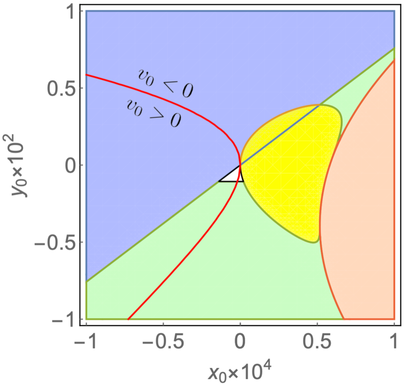
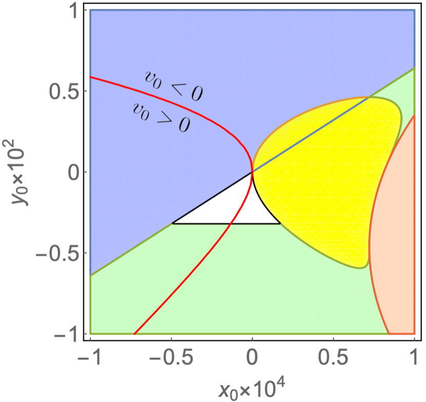
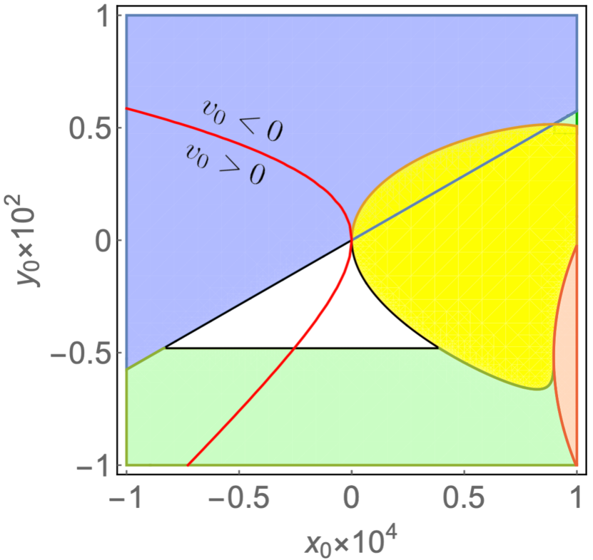
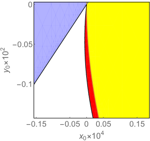
It is useful to note that the asymptotics of and may be chosen in such a way that
| (32) |
This is possible for all allowed values of . In what follows we consider this case only.
3.2.2 Inflation after bounce
As outlined in the beginning of this Section, our next step is to describe the inflationary stage, and then discuss the transition from contraction to inflation through bounce. Models of inflation in the Horndeski theory have been proposed in Refs. [3, 54, 10, 12, 61, 62]; here we employ the construction similar to Ref. [24]. Namely, exact exponential expansion occurs when the functions in the Lagrangian take constant values,
| (33a) | ||||
| (33b) | ||||
where the choice (33a) is made to restore GR already at inflation (recall that ). With the Ansatz (33), equations of motion (21) read
| (34a) | |||
| (34b) | |||
and we denote the (time-independent) solution to these equations by and . We require , .
Now, it is convenient to consider , , and as independent parameters, and express and through these parameters using (34):
| (35a) | ||||
| (35b) | ||||
Let us turn to the requirements of background stability and subluminal propagation of perturbations. Using (22) and (35), we arrive at the constraints
These constraints can be written in a simple form:
| (36a) | ||||
| (36b) | ||||
which also leads to
| (37) |
It is worth noting that the value of at inflation has the opposite sign to its value at contraction: [see Eq. (36a)] and (see Fig. 1), respectively. On the contrary, the values of and have the same signs at these two stages, see Eqs. (32) and (37).
Now, let us comment on the possible behavior of the functions , , and near the bounce. Since and do not change signs during the transition from contraction to inflation, it is natural to take them monotonously changing from to and from to , respectively. The function flattens out, with both at contraction and bounce. Near the bounce, at , we have . Assuming that the functions and vary slowly in comparison with in the vicinity of the bounce, we obtain from the first equation of motion, Eq. (21a) with , that
| (38) |
We note in passing that with our choice of signs of and at contraction, inflation and bounce (, ), the argument of square root is positive. Then, we take the time derivative of Eq. (21a) and solve it together with Eq. (21b) for and to find
where we again neglect , , and in comparison with . Since , we see that may be negative, but only slightly:
With this qualification, most of the smooth functions interpolating between (24) and (33) indeed give rise to the bouncing solution. We present a numerical example in Sec. 3.2.4.
3.2.3 Kination epoch after transit from inflation
To describe the final kination epoch with GR and free massless scalar field, we make use of the covariant formalism with the Lagrangian (3). It is convenient to use the freedom of field redefinition and choose the background field as follows:
| (39) |
This choice corresponds to the Lagrangian
Indeed, it is straightforward to check that the scalar field equation and Friedmann equation have the solution (39) with , , and . Note that during the transition from inflation to kination, the coefficient of in the Lagrangian changes sign (it changes from at inflation to at kination). This is in complete accordance with [50, 51].
Towards the kination epoch, other terms in the scalar field Lagrangian should tend sufficiently rapidly to zero. This can be achieved, e.g., by requiring the following asymptotics of functions in the covariant Lagrangian (3) at large (distant future; recall that GR is restored already at inflation, ):
| (40a) | ||||
| (40b) | ||||
where and are damping factors, which suppress higher order terms. They can be chosen rather arbitrarily. We choose them as follows:
The reason for this choice is that we obtain simple ADM functions and using conversion formulas (6)–(9):
In fact, we have to generalize these expressions by introducing time shift, , where is a new parameter. The point is that once contraction is described literally by formulas of Sec. 3.2.1, inflation begins soon after and ends at some much later time . The time shift (with of order of but somewhat smaller than ) has to be introduced to account for the fact that kination begins around . Thus, the asymptotic behavior of , , and at large is (recall that at inflation and later)
| (41a) | ||||
| (41b) | ||||
| (41c) | ||||
By choosing the functions , , and in such a way that they interpolate between constant values , , and at inflation and functions (41) at late times, we obtain a smooth transition from inflation to kination. The issues of stability and subluminality are, however, tricky at transition epochs; designing a completely stable and subluminal model requires considerable trial and error effort.
3.2.4 Numerical example
Here we present a concrete model which proves by example that there exists stable and subluminal cosmology with the desired properties listed in the beginning of this Section. We emphasize again that by rescaling the functions in the Lagrangian in accordance with Eq. (16), one can make all time scales like , inverse inflationary Hubble parameter , etc., arbitrarily long, much longer than the Planck time. This observation applies also to other models considered in this paper.
We choose the parameter near the center of allowed interval :
As we already mentioned, at the contracting stage we choose, quite arbitrarily,
| (42) |
The parameters and are then chosen from the allowed region shown in Fig. 1; by trial and error we find convenient values, consistent with the sign choice (32):
| (43) |
The value of and the Hubble coefficient at the contraction stage are found from (26) and (27):
| (44) |
This completes the description of the contraction stage.
We would like to have bounce at some time before ; we request [although we do not have to do so in view of scaling (16)] that the characteristic time scales are large compared to 1 (i.e., Planck time). We begin with the function which should interpolate between at contraction and at inflation. A simple choice is
| (45) |
The parameter is the inverse time scale of the transition, and we set
| (46) |
We wish the bounce to occur roughly at , so the maximum value of at contraction is estimated as
Let us now turn to the inflationary stage and transition to it. A simple Ansatz for the inflationary Hubble parameter is that it is comparable to the maximum value at contraction. There is no reason to think that the lapse function at inflation is considerably different from 1. We choose
We also have to specify the value of at inflation. To this end, we introduce a simple Ansatz of proportionality between and :
| (47) |
so that is time independent at the transition from contraction to inflation. Note that with the numerical values (43) and (44), the estimate (38) is consistent with our choice . Equation (47) implies , then (35) gives
and numerically
This set of parameters is consistent with the stability and subluminality constraints (36). The values of and are found from (35):
Note that , , and are much smaller than , , and , respectively. This has to do with two properties of the contracting stage which distinguish it from inflation. First, the constraints shown in Fig. 1 are consistent with fairly large values of , and it is indeed quite large in our example; on the contrary, inflationary is bounded by , see (36b). Second, equation of motion (21b) contains a term proportional to , which is not so small at contraction and drives and to fairly large values; this term vanishes at inflation. We note in passing that Eq. (21a) is satisfied at the contraction stage due to the partial cancellation between and .
The transition from contraction through bounce to inflation is described by , , and smoothly interpolating between , , and , , [and with given by (45)]. A nontrivial part of the construction is to make sure that stability and subluminality conditions (14) and (15) are satisfied. By trial and error, we find appropriate forms
| (48a) | ||||
| (48b) | ||||
where the functions
| (49a) | ||||
| (49b) | ||||
interpolate between 0 and 1, while is given by (47), and the parameter is the same as in (46).
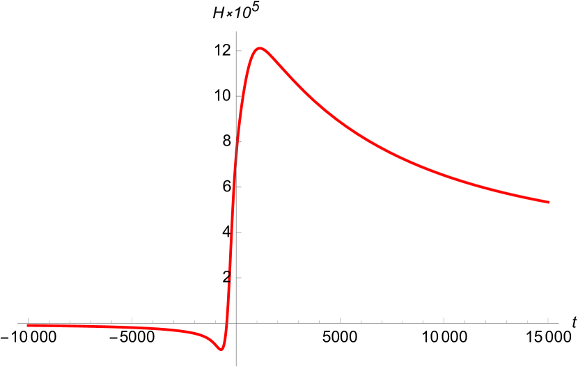
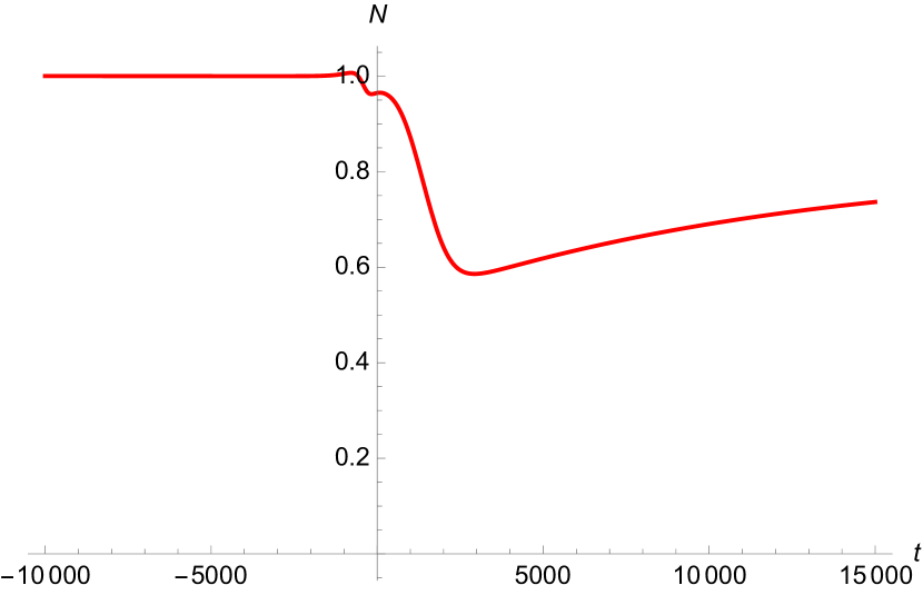
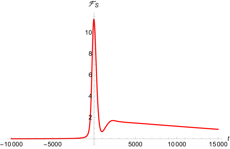
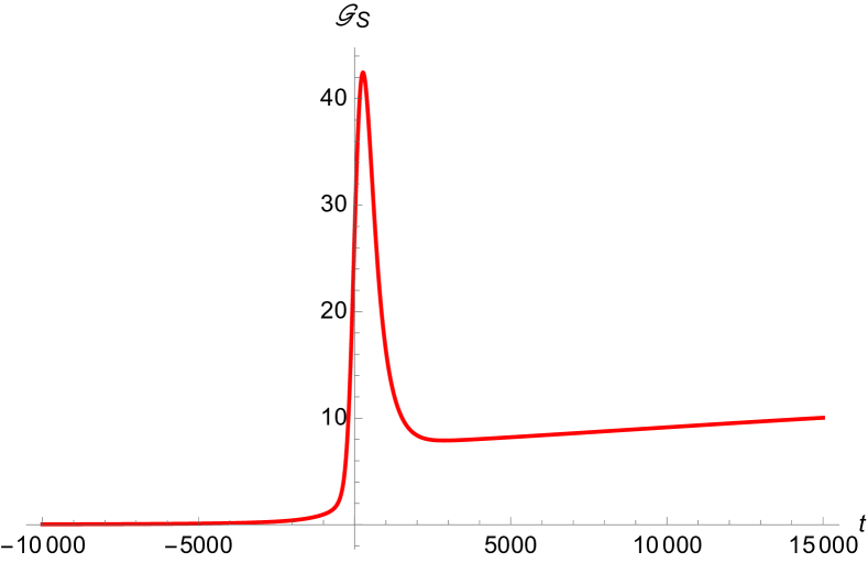
We show the behavior of the Hubble parameter and lapse function at contraction, bounce, and beginning of inflation in Fig. 3. The scalar coefficients and and scalar sound speed are shown in Figs. 4, 4 and 5, respectively; the stability and subluminality are explicit. We show tensor coefficient for completeness in Fig. 5 (recall that and at all times).
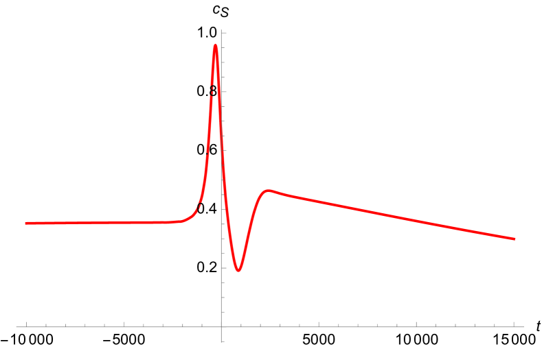
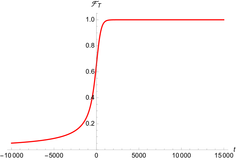
So, after a rather short transition period, the inflationary stage sets in. Depending on the parameters of the model, it can last for a longer or shorter time. Note that this property may be of interest from a phenomenological viewpoint [62]. We take, quite arbitrarily, the duration of inflation approximately equal to (in Planck units), which corresponds to the number of e-foldings at inflation .
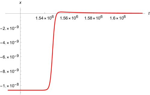
To have the transition from inflation to kination, we take at late times
| (50a) | ||||
| (50b) | ||||
| (50c) | ||||
with the parameter which regulates the duration of inflation equal to , and
where , and the function
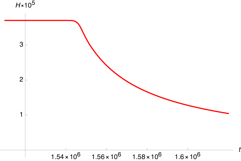
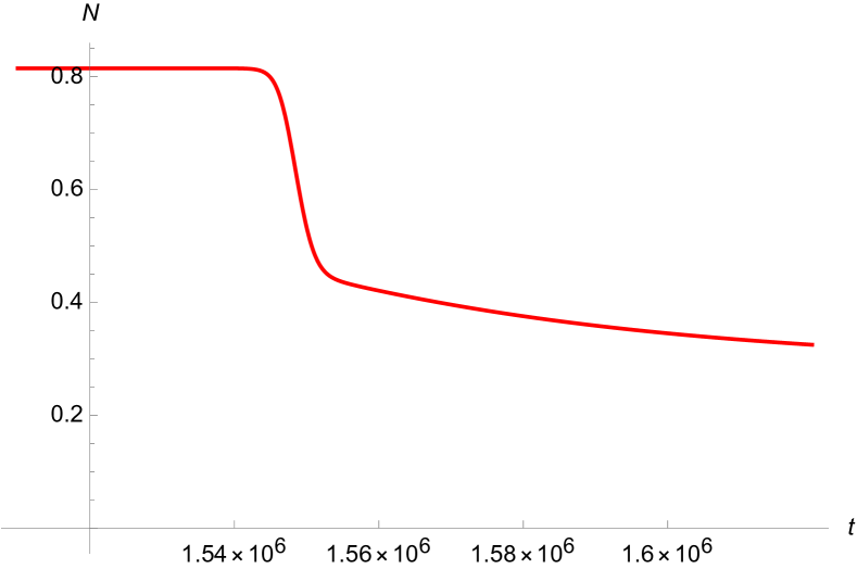
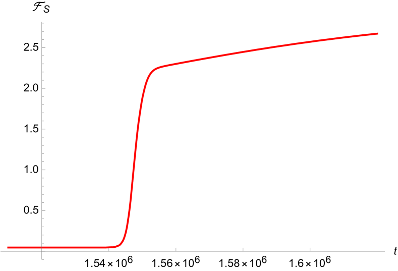
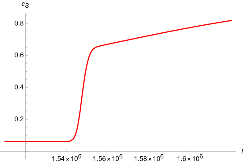
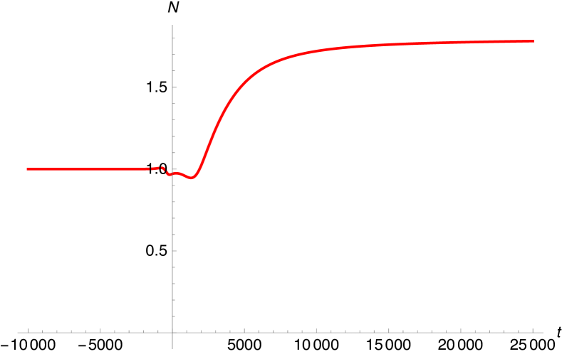
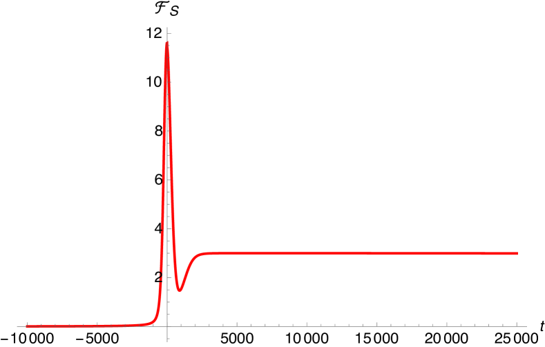
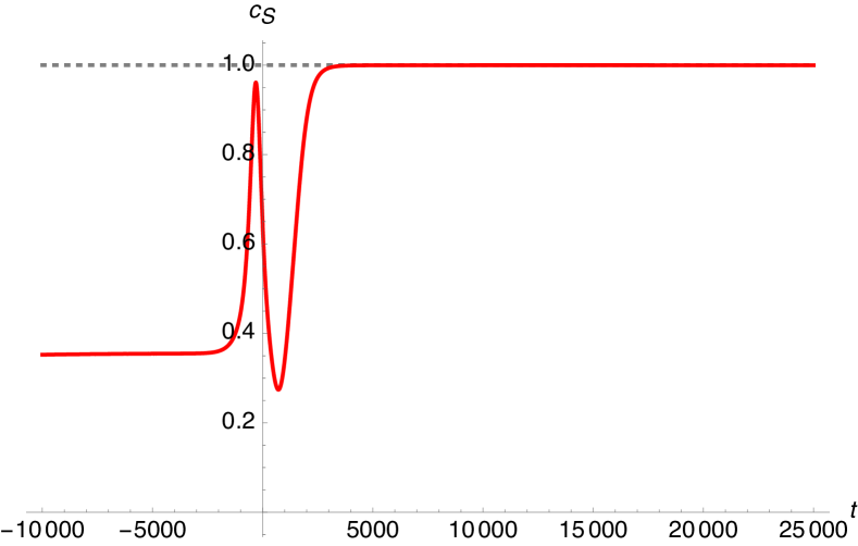
again interpolates between 0 and 1 [the value of parameter is still given by (46)]. The parameters and are chosen in such a way that the functions , , and are reasonably smooth in the transition period, and inflation smoothly ends somewhat later than . This is illustrated in Fig. 6. At late times we obtain the correct kination behavior given by (41), and the Hubble parameter asymptotes to . The Hubble parameter and lapse function are shown in Fig. 7, while the scalar coefficient and scalar sound speed are shown in Fig. 8. Clearly, the model is stable and subluminal at the transition from inflation to kination. The sound speed tends to 1 rather slowly, since the ratio exhibits slow decay (and decays as ).
3.3 Bounce directly to kination
Contraction and bounce need not necessarily proceed into the inflationary stage: a short transition epoch after bounce may end up directly at kination. In this scenario, the initial stage is described in the same way as in Sec. 3.2.1, whereas the evolution after bounce proceeds as in Sec. 3.2.3. Let us give a numerical example which shows that stable and subluminal cosmology of this sort is indeed possible.
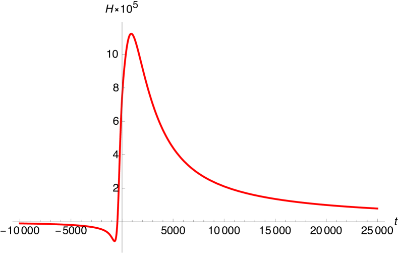
We again consider a model with and choose the parameters of the contraction stage as in (42), (43), and (44). The function is again given by (45), so that we restore GR at later times. We would like to approach the behavior (41) soon after bounce and, by trial and error, end up with the following example:
where and are still given by (49), and now
We show the Hubble parameter and lapse function for this model in Fig. 9 and the scalar coefficient and scalar sound speed in Fig. 10. The latter figure illustrates that the model is stable and subluminal at all times.
4 Models with genesis
4.1 Ansatz
To illustrate that interesting cosmologies can be obtained within various Ansätze, in this Section we construct genesis models by choosing the functions in the Lagrangian (5) in the following form:
| (52a) | |||
| (52b) | |||
| (52c) | |||
| (52d) | |||
The parameter is similar to that in the previous Section, and the parameter is new. The functions and depend on now; functions , , , and are chosen as follows:
| (53a) | |||
| (53b) | |||
| (53c) | |||
| (53d) | |||
Note that the parameter is now time independent, unlike in the models of Sec. 3 where functions and entering exhibited step-function behavior.
4.2 Contracting genesis followed by bounce
Here we construct a model with genesis of contracting Universe. This cosmology begins with the flat space-time, then the Universe starts to contract, and the rate of contraction increases. At some moment of time the bounce occurs: the contraction terminates and expansion begins. We consider for definiteness the case in which bounce is followed by inflationary expansion; inflation is assumed to end up as in Sec. 3.2. Alternatively, bounce may lead directly to kination epoch like in Sec. 3.3; we do not elaborate on this possibility.
We begin with early times and consider the following asymptotics
| (56a) | |||
| (56b) |
This choice leads to power-law behavior of the Hubble parameter. Indeed, by substituting (56) into equations of motion (54) we arrive at
with
| (57) |
[the fact that for this solution is due to the particular choice of the coefficient of in (53a); this choice replaces in this model the constraint (26)]. For , the scale factor tends to a constant as :
as required for genesis. Contracting genesis occurs for .
Let us note that for small , early time asymptotics is approached slowly (backwards in time), since the expansion parameter is :
| (58a) | ||||
| (58b) | ||||
where coefficients and are not particularly small. This complicates the numerical analysis; we explain how we get around this obstacle in Appendix B. The same comment applies to the genesis model of Sec. 4.3.
The asymptotic behavior of coefficients (55) entering the quadratic action for perturbations is
The constraints on parameters arise from the same requirements as in Sec. 3.2.1. Let us list them:
(i) Contraction at early times:
| (59) |
(ii) Stability of background and subluminality of perturbations:
| (60a) | |||
| (60b) | |||
(iii) Evading the no-go argument of Ref. [24]:
| (61) |
(iv) Absence of strong coupling in the past. This issue has been studied in detail in Ref. [47] with the result
| (62) |
(v) Belinsky–Khalatnikov–Lifshitz phenomenon. In the same way as in Sec. 3, we obtain for time-dependent superhorizon perturbations
and
They decay as increases towards zero, provided that . This constraint is weaker than (iii).
All these constraints can be satisfied without much of fine-tuning. In view of (61), the constraints give
and gives
The constraint is satisfied automatically. This set of inequalities can be satisfied for all and from their allowed range.
Let us turn to inflationary epoch. Like in Sec. 3.2, inflation occurs for time-independent coefficients in the Lagrangian:
| (63a) | ||||
| (63b) | ||||
In this case, equations of motion (54) read
| (64a) | |||
| (64b) | |||
and we denote the (time-independent) solution to these equations by and . We require , .
In analogy to Sec. 3.2, it is convenient to treat and as independent parameters and express and through these parameters using (64):
| (65a) | ||||
| (65b) | ||||
We emphasize that unlike in the bounce scenario of Sec. 3, the inflationary epoch in our current model is not described by GR since . The conditions for the background stability and subluminal propagation of perturbations, Eqs. (55), read
| (66a) | ||||
| (66b) | ||||
| (66c) | ||||
| (66d) | ||||
| (66e) | ||||
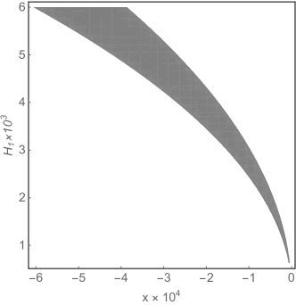
These can also be satisfied without much of fine-tuning. As an example, the allowed range of and is shown in Fig. 11 for rather arbitrarily chosen , , and . Plots for other values of are similar, provided that . The fact that is negative and is small for small (inflationary expansion rate much lower than the Planck scale) is clear from, e.g., Eq. (66b).
To see that the contracting genesis stage can consistently pass through bounce to inflationary expansion, we now give an explicit numerical example. As we alluded to above, we choose , . The parameter relevant to the contracting genesis stage is chosen as . By trial and error we find convenient values for other Lagrangian parameters at early times, consistent with the system of constraints (59)-(62) and (66):
| (67) |
The value of the Hubble coefficient at the contraction stage is found from (57), . Next, we turn to the function which should interpolate between at contraction and at inflation. To ensure stability and subluminality at all times, we choose this function in somewhat more complicated form than in (45):
where
interpolates between and . The parameter is the same as in (46), .
We now define the parameters of the inflationary stage and describe transition to it through bounce. We choose the (time-independent) Hubble parameter and lapse function at inflation as follows:
This set of parameters is consistent with the stability and subluminality constraints (66). Then Eq. (65) with given by (67) leads to
| (68) |
The transition from contraction to inflation is described by and smoothly interpolating between , and , . By trial and error, we find appropriate functions
| (69a) | ||||
| (69b) | ||||
where the functions
interpolate between 0 and 1. A nontrivial requirement leading to (69) is again stability and subluminality of perturbations at all times.
We show the behavior of the Hubble parameter and lapse function at contraction, bounce and beginning of inflation in Fig. 12. The scalar coefficient and scalar sound speed are shown in Fig. 13: the stability and subluminality are explicit (although not obvious in Fig. 13a, the coefficient is, in fact, strictly positive at all times).
We end up this Section by the following remark. As we pointed out above, gravity at the inflationary epoch is not yet described by GR, since and, therefore , see Eqs. (53c), (53d). To ensure that inflation at its last stage proceeds within GR, one chooses which, at the intermediate inflationary stage, smoothly evolves from to . The function should also be nontrivial, as it should interpolate between the negative value [see (68)] and some positive value . The latter property follows from the expression for , which for has the following form:
where and are lapse function and Hubble parameter at GR inflation. It is straightforward to design appropriate functions and without spoiling the stability and subluminality properties. An example is
where , and
The transition from late GR inflation to kination proceeds in the same way as in Sec. 3.2.
4.3 Genesis without strong coupling
As we pointed out in the Introduction, the genesis model of Ref. [24] suffers from the strong coupling problem at early times. For completeness, we present here a version of this model which is free of the strong coupling problem. The Lagrangian is the same as in [24] but with different parameters. Namely, the Lagrangian functions are defined by Ansatz (52) with , , and , i.e.,
| (70a) | |||
| (70b) | |||
| (70c) | |||
where , and
As before, we choose the asymptotic behavior () as , and using equation of motion (54) obtain the genesis behavior
| (71) |
where is given by
The asymptotics of the scalar coefficients and scalar sound speed squared are
Parameters of this model should obey several constraints. The first one comes from the requirement of evading the no-go argument of Ref. [24]:
| (72) |
The second constraint ensures that the classical treatment of early time evolution is legitimate [47]:
| (73) |
The third one is the requirement that the Universe expands at early times:
| (74) |
Finally, one requires the background stability and subluminal propagation of perturbations. For (as needed for healthy inflation, see below), all these constraints are satisfied, provided that and
| (75) |
The transition from the genesis stage to inflation is achieved simply by flattening out the function to . For , equations of motion (54) read
| (76a) | |||
| (76b) | |||
and we denote the (time-independent) solution to these equations by and . We require , . The requirements of background stability and subluminal propagation of perturbations, Eqs. (55), read in this case
| (77a) | ||||
| (77b) | ||||
As before, it is convenient to treat and as independent parameters and express and through these parameters using (76):
| (78a) | ||||
| (78b) | ||||
Then the constraints (75) and (77) reduce to
| (79a) | ||||
| (79b) | ||||
In accordance with (78), these constraints translate into constraints on and . It is straightforward to see that the latter are satisfied, provided that and obeys (75).
Now, let us turn to our numerical example. We choose
This choice is consistent with the constraints (72) and (73). We choose
We obtain the values of and by considering the inflationary stage. We choose and at inflation as follows:
This set of parameters is consistent with constraints (79). Then Eq. (78) leads to
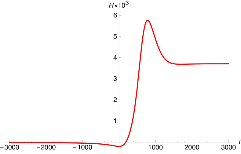
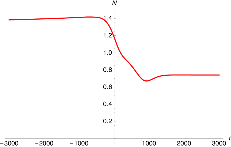
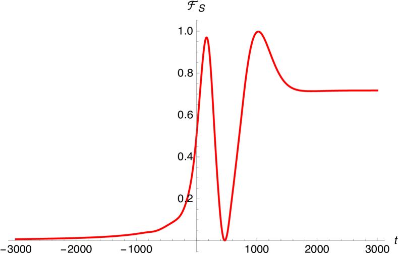
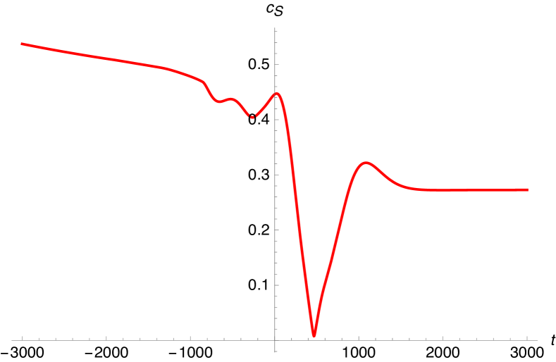
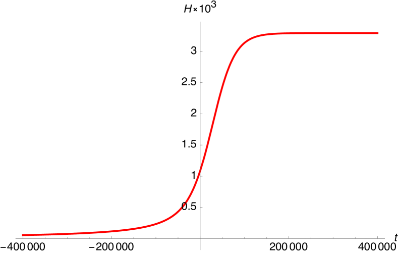
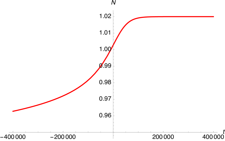
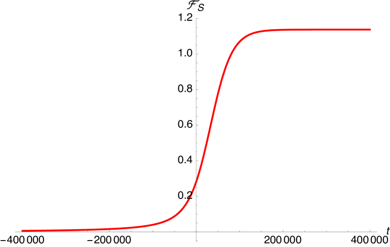
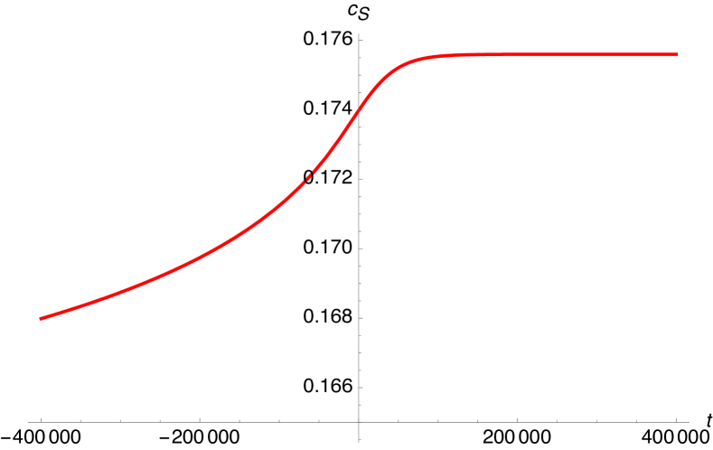
which is consistent with (75). We show the evolution of the Hubble parameter, lapse function, scalar coefficient , and scalar sound speed in Figs. 14 and 15. In the tensor sector we have , . Thus, our background solution is fully stable and free of the strong coupling problem at early times; perturbations about it are not superluminal. We conclude that our model gives an example of healthy genesis with strong gravity in the past.
5 Conclusion
This paper demonstrates that it is relatively straightforward to construct, within the Horndeski class of scalar-tensor theories, nonsingular cosmological models which are healthy, i.e., free of instabilities and superluminal propagation of perturbations. The price to pay is strong gravity in the past, the property that effective Planck masses tend to zero as . We have made sure, however, that the latter property does not spoil the description of the background within classical field theory. In this way we have constructed bouncing models, genesis cosmology, and a combination thereof. These may or may not pass through the inflationary stage, as we explicitly demonstrated in Sec. 3.
In our constructions, we heavily exploited the functional freedom that exists in the Horndeski class of theories. On the one hand, this freedom is instrumental for designing models with prescribed properties (in other words, for employing the ‘‘inverse method’’ [21]); on the other, it makes the whole approach not so appealing. It is certainly desirable to have a better idea of which Horndeski theories, if any, have a chance to be realistic as low energy effective theories.
Acknowledgments
The authors are grateful to Victoria Volkova and Sergei Mironov for useful comments and fruitful discussions. This work has been supported by Russian Science Foundation Grant No. 19-12-00393.
Appendix A ABSENCE OF STRONG COUPLING AT EARLY TIMES
The purpose of this Appendix is to study the issue of strong coupling at early times in the model with the Lagrangian (5) and (19) and contracting background solution (23) and (24). As we outlined in Sec. 1, we are going to compare the energy scale of classical evolution with quantum strong coupling scale inferred from the analysis of the nonlinear terms in the Lagrangian for perturbations about this background. We begin with the action written in terms of metric variables,
with the Lagrangian (5) (recall that denotes the background lapse function). Different terms in the Lagrangian (5) contain different powers of the scale factor, which in the contracting Universe nontrivially depends on time, . It is therefore convenient to work with physical momenta and frequencies. Assuming that they are higher than , i.e., assuming that , we can neglect slow dependence of the scale factor on and at a given time treat as an (instantaneously) time-independent parameter (with the exception of expressions that involve the Hubble parameter explicitly). Of course, this assumption must be justified a posteriori: the whole analysis is valid if the classical treatment of the background is legitimate, . Having this in mind, we introduce physical spatial and temporal coordinates
Note that in our case, but we keep the notation for concordance with spatial coordinates. Then the derivatives are, respectively,
| (A.1a) | ||||
| (A.1b) | ||||
We now rewrite our Lagrangian (5) in terms of physical coordinates. We define
| (A.2) |
and find
| (A.3) |
where ,
| (A.4) |
the new (physical) transverse shift vector is given by
and (and below) are made of metric . We rewrite in the same way:
| (A.5) |
Finally, we have . Thus, the action written in terms of physical variables does not contain the scale factor anymore, but otherwise the Lagrangian has the same structure as the original one (5), except for the first term in the right-hand side of (A.4).
The action for perturbations, written in terms of physical variables , , is identically the same as the limiting case of the action that we encountered in Ref. [47], where we studied the strong coupling issue in the model with genesis described in Sec. 4.3. Namely, the model with genesis has an additional parameter in (70), while the bouncing model we discuss does not. By direct inspection we find that the action for perturbations in the bouncing model, written in terms of physical variables, is obtained from the action for perturbations in the genesis model by sending [this includes also the first term in the right-hand side of (A.4)]. Thus, the sufficient condition for the absence of the strong coupling problem is obtained from the result of Ref. [47] in the limit and reads
This result is quoted in Sec. 3.
Let us illustrate this constraint by considering the quadratic and cubic action for tensor modes. The complete expression is [63]
We recall that , see (28a). To figure out the associated strong coupling scale, we introduce the canonically normalized field (omitting indices)
and find that the interaction term is (modulo numerical factor)
Thus, on dimensional grounds, the strong coupling scale is
This scale is much higher than the classical scale for , as promised.
Appendix B CONTRACTING GENESIS: SUBTLETY OF NUMERICAL SOLUTION
As we pointed out in Sec. 4.2, corrections to the leading asymptotics of classical solutions at early times behave as . This makes straightforward numerical treatment problematic for small . Here we sketch our way of dealing with this problem. We consider for definiteness the model of Sec. 4.2 with .
We study the time interval , where is negative and is large enough, so that it is a very good approximation to use the asymptotics
| (B.1) |
(recall that these asymptotics are approached exponentially fast backwards in time). We introduce a new variable instead of :
| (B.2) |
early-time asymptotics occur as . Then corrections to the leading asymptotics of classical solutions are of order . The key point is to introduce, instead of , a new unknown function as follows:
Then coefficient factors out in equations of motion (54), and coefficients in these equations become linear polynomials in . This form of equations of motion enables one to solve them in a straightforward way.
The initial condition in distant past is set by expanding and in at small . The first nontrivial terms in this expansion are straightforward to calculate. One writes, in notations (58),
and
For our choice of parameters , , and in (67), and , , and , the coefficients are
Thus, corrections are small for small enough , where initial conditions are imposed. In practice we choose , which corresponds to . This huge number is the reason why we have invented our procedure.
We solve the equations of motion written in terms of until becomes roughly of order 1; in practice we choose , so that . At that time Eq. (B.1) is still a good approximation. Then we continue solving equations of motion using time , with obvious matching at .
References
- [1] P. Creminelli, A. Nicolis and E. Trincherini, JCAP 11, 021 (2010) doi:10.1088/1475-7516/2010/11/021 [arXiv:1007.0027 [hep-th]].
- [2] C. Deffayet, O. Pujolas, I. Sawicki and A. Vikman, JCAP 10, 026 (2010) doi:10.1088/1475-7516/2010/10/026 [arXiv:1008.0048 [hep-th]].
- [3] T. Kobayashi, M. Yamaguchi and J. Yokoyama, Phys. Rev. Lett. 105, 231302 (2010) doi:10.1103/PhysRevLett.105.231302 [arXiv:1008.0603 [hep-th]].
- [4] G. W. Horndeski, Int. J. Theor. Phys. 10, 363-384 (1974) doi:10.1007/BF01807638
- [5] V. A. Rubakov, Phys. Usp. 57, 128-142 (2014) doi:10.3367/UFNe.0184.201402b.0137 [arXiv:1401.4024 [hep-th]].
- [6] T. Kobayashi, Rept. Prog. Phys. 82, no.8, 086901 (2019) doi:10.1088/1361-6633/ab2429 [arXiv:1901.07183 [gr-qc]].
- [7] P. Creminelli, K. Hinterbichler, J. Khoury, A. Nicolis and E. Trincherini, JHEP 02, 006 (2013) doi:10.1007/JHEP02(2013)006 [arXiv:1209.3768 [hep-th]].
- [8] K. Hinterbichler, A. Joyce, J. Khoury and G. E. J. Miller, JCAP 12, 030 (2012) doi:10.1088/1475-7516/2012/12/030 [arXiv:1209.5742 [hep-th]].
- [9] B. Elder, A. Joyce and J. Khoury, Phys. Rev. D 89, no.4, 044027 (2014) doi:10.1103/PhysRevD.89.044027 [arXiv:1311.5889 [hep-th]].
- [10] D. Pirtskhalava, L. Santoni, E. Trincherini and P. Uttayarat, JHEP 12, 151 (2014) doi:10.1007/JHEP12(2014)151 [arXiv:1410.0882 [hep-th]].
- [11] S. Nishi and T. Kobayashi, JCAP 03, 057 (2015) doi:10.1088/1475-7516/2015/03/057 [arXiv:1501.02553 [hep-th]].
- [12] T. Kobayashi, M. Yamaguchi and J. Yokoyama, JCAP 07, 017 (2015) doi:10.1088/1475-7516/2015/07/017 [arXiv:1504.05710 [hep-th]].
- [13] T. Qiu, J. Evslin, Y. F. Cai, M. Li and X. Zhang, JCAP 10, 036 (2011) doi:10.1088/1475-7516/2011/10/036 [arXiv:1108.0593 [hep-th]].
- [14] D. A. Easson, I. Sawicki and A. Vikman, JCAP 11, 021 (2011) doi:10.1088/1475-7516/2011/11/021 [arXiv:1109.1047 [hep-th]].
- [15] Y. F. Cai, D. A. Easson and R. Brandenberger, JCAP 08, 020 (2012) doi:10.1088/1475-7516/2012/08/020 [arXiv:1206.2382 [hep-th]].
- [16] M. Osipov and V. Rubakov, JCAP 11, 031 (2013) doi:10.1088/1475-7516/2013/11/031 [arXiv:1303.1221 [hep-th]].
- [17] T. Qiu, X. Gao and E. N. Saridakis, Phys. Rev. D 88, no.4, 043525 (2013) doi:10.1103/PhysRevD.88.043525 [arXiv:1303.2372 [astro-ph.CO]].
- [18] M. Koehn, J. L. Lehners and B. A. Ovrut, Phys. Rev. D 90, no.2, 025005 (2014) doi:10.1103/PhysRevD.90.025005 [arXiv:1310.7577 [hep-th]].
- [19] L. Battarra, M. Koehn, J. L. Lehners and B. A. Ovrut, JCAP 07, 007 (2014) doi:10.1088/1475-7516/2014/07/007 [arXiv:1404.5067 [hep-th]].
- [20] T. Qiu and Y. T. Wang, JHEP 04, 130 (2015) doi:10.1007/JHEP04(2015)130 [arXiv:1501.03568 [astro-ph.CO]].
- [21] A. Ijjas and P. J. Steinhardt, Phys. Rev. Lett. 117, no.12, 121304 (2016) doi:10.1103/PhysRevLett.117.121304 [arXiv:1606.08880 [gr-qc]].
- [22] D. A. Dobre, A. V. Frolov, J. T. Gálvez Ghersi, S. Ramazanov and A. Vikman, JCAP 03, 020 (2018) doi:10.1088/1475-7516/2018/03/020 [arXiv:1712.10272 [gr-qc]].
- [23] M. Libanov, S. Mironov and V. Rubakov, JCAP 08, 037 (2016) doi:10.1088/1475-7516/2016/08/037 [arXiv:1605.05992 [hep-th]].
- [24] T. Kobayashi, Phys. Rev. D 94, no.4, 043511 (2016) doi:10.1103/PhysRevD.94.043511 [arXiv:1606.05831 [hep-th]].
- [25] R. Kolevatov and S. Mironov, Phys. Rev. D 94, no.12, 123516 (2016) doi:10.1103/PhysRevD.94.123516 [arXiv:1607.04099 [hep-th]].
- [26] S. Akama and T. Kobayashi, Phys. Rev. D 95, no.6, 064011 (2017) doi:10.1103/PhysRevD.95.064011 [arXiv:1701.02926 [hep-th]].
- [27] A. Ijjas, F. Pretorius and P. J. Steinhardt, JCAP 01, 015 (2019) doi:10.1088/1475-7516/2019/01/015 [arXiv:1809.07010 [gr-qc]].
- [28] G. Papallo and H. S. Reall, Phys. Rev. D 96, no.4, 044019 (2017) doi:10.1103/PhysRevD.96.044019 [arXiv:1705.04370 [gr-qc]].
- [29] G. Allwright and L. Lehner, Class. Quant. Grav. 36, no.8, 084001 (2019) doi:10.1088/1361-6382/ab0ee1 [arXiv:1808.07897 [gr-qc]].
- [30] Á. D. Kovács, Phys. Rev. D 100, no.2, 024005 (2019) doi:10.1103/PhysRevD.100.024005 [arXiv:1904.00963 [gr-qc]].
- [31] P. Creminelli, M. A. Luty, A. Nicolis and L. Senatore, JHEP 12, 080 (2006) doi:10.1088/1126-6708/2006/12/080 [arXiv:hep-th/0606090 [hep-th]].
- [32] M. Koehn, J. L. Lehners and B. Ovrut, Phys. Rev. D 93, no.10, 103501 (2016) doi:10.1103/PhysRevD.93.103501 [arXiv:1512.03807 [hep-th]].
- [33] C. de Rham and S. Melville, Phys. Rev. D 95, no.12, 123523 (2017) doi:10.1103/PhysRevD.95.123523 [arXiv:1703.00025 [hep-th]].
- [34] Y. Cai, Y. Wan, H. G. Li, T. Qiu and Y. S. Piao, JHEP 01, 090 (2017) doi:10.1007/JHEP01(2017)090 [arXiv:1610.03400 [gr-qc]].
- [35] P. Creminelli, D. Pirtskhalava, L. Santoni and E. Trincherini, JCAP 11, 047 (2016) doi:10.1088/1475-7516/2016/11/047 [arXiv:1610.04207 [hep-th]].
- [36] Y. Cai and Y. S. Piao, JHEP 09, 027 (2017) doi:10.1007/JHEP09(2017)027 [arXiv:1705.03401 [gr-qc]].
- [37] R. Kolevatov, S. Mironov, N. Sukhov and V. Volkova, JCAP 08, 038 (2017) doi:10.1088/1475-7516/2017/08/038 [arXiv:1705.06626 [hep-th]].
- [38] S. Mironov, V. Rubakov and V. Volkova, Phys. Rev. D 100, no.8, 083521 (2019) doi:10.1103/PhysRevD.100.083521 [arXiv:1905.06249 [hep-th]].
- [39] M. Zumalacárregui and J. García-Bellido, Phys. Rev. D 89, 064046 (2014) doi:10.1103/PhysRevD.89.064046 [arXiv:1308.4685 [gr-qc]].
- [40] J. Gleyzes, D. Langlois, F. Piazza and F. Vernizzi, Phys. Rev. Lett. 114, no.21, 211101 (2015) doi:10.1103/PhysRevLett.114.211101 [arXiv:1404.6495 [hep-th]].
- [41] D. Langlois and K. Noui, JCAP 02, 034 (2016) doi:10.1088/1475-7516/2016/02/034 [arXiv:1510.06930 [gr-qc]].
- [42] D. Langlois, Int. J. Mod. Phys. D 28, no.05, 1942006 (2019) doi:10.1142/S0218271819420069 [arXiv:1811.06271 [gr-qc]].
- [43] S. Mironov, V. Rubakov and V. Volkova, JHEP 04, 035 (2021) doi:10.1007/JHEP04(2021)035 [arXiv:2011.14912 [hep-th]].
- [44] A. Ijjas and P. J. Steinhardt, Phys. Lett. B 764, 289-294 (2017) doi:10.1016/j.physletb.2016.11.047 [arXiv:1609.01253 [gr-qc]].
- [45] Y. A. Ageeva, O. A. Evseev, O. I. Melichev and V. A. Rubakov, EPJ Web Conf. 191, 07010 (2018) doi:10.1051/epjconf/201819107010 [arXiv:1810.00465 [hep-th]].
- [46] Y. Ageeva, O. Evseev, O. Melichev and V. Rubakov, Phys. Rev. D 102, no.2, 023519 (2020) doi:10.1103/PhysRevD.102.023519 [arXiv:2003.01202 [hep-th]].
- [47] Y. Ageeva, P. Petrov and V. Rubakov, JHEP 12, 107 (2020) doi:10.1007/JHEP12(2020)107 [arXiv:2009.05071 [hep-th]].
- [48] P. K. Petrov, Mod. Phys. Lett. A 35, no.37, 2050305 (2020) doi:10.1142/S0217732320503058 [arXiv:2004.13123 [hep-th]].
- [49] B. Bellazzini, J. Elias Miró, R. Rattazzi, M. Riembau and F. Riva, [arXiv:2011.00037 [hep-th]].
- [50] C. Armendariz-Picon, T. Damour and V. F. Mukhanov, Phys. Lett. B 458, 209-218 (1999) doi:10.1016/S0370-2693(99)00603-6 [arXiv:hep-th/9904075 [hep-th]].
- [51] H. Bazrafshan Moghaddam, R. Brandenberger and J. Yokoyama, Phys. Rev. D 95, no.6, 063529 (2017) doi:10.1103/PhysRevD.95.063529 [arXiv:1612.00998 [hep-th]].
- [52] J. Gleyzes, D. Langlois, F. Piazza and F. Vernizzi, JCAP 08, 025 (2013) doi:10.1088/1475-7516/2013/08/025 [arXiv:1304.4840 [hep-th]].
- [53] M. Fasiello and S. Renaux-Petel, JCAP 10, 037 (2014) doi:10.1088/1475-7516/2014/10/037 [arXiv:1407.7280 [astro-ph.CO]].
- [54] T. Kobayashi, M. Yamaguchi and J. Yokoyama, Prog. Theor. Phys. 126, 511-529 (2011) doi:10.1143/PTP.126.511 [arXiv:1105.5723 [hep-th]].
- [55] A. Adams, N. Arkani-Hamed, S. Dubovsky, A. Nicolis and R. Rattazzi, JHEP 10, 014 (2006) doi:10.1088/1126-6708/2006/10/014 [arXiv:hep-th/0602178 [hep-th]].
- [56] C. de Rham, M. Fasiello and A. J. Tolley, Phys. Lett. B 733, 46-51 (2014) doi:10.1016/j.physletb.2014.03.061 [arXiv:1308.2702 [hep-th]].
- [57] E. M. Lifshitz and I. M. Khalatnikov, Adv. Phys. 12, 185-249 (1963) doi:10.1080/00018736300101283
- [58] V. A. Belinsky, I. M. Khalatnikov and E. M. Lifshitz, Adv. Phys. 19, 525-573 (1970) doi:10.1080/00018737000101171
- [59] V. A. Belinskii, E. M. Lifshitz and I. M. Khalatnikov, Zh. Eksp. Teor. Fiz. 62, 1606-1613 (1972)
- [60] J. K. Erickson, D. H. Wesley, P. J. Steinhardt and N. Turok, Phys. Rev. D 69, 063514 (2004) doi:10.1103/PhysRevD.69.063514 [arXiv:hep-th/0312009 [hep-th]].
- [61] S. Hirano, T. Kobayashi and S. Yokoyama, Phys. Rev. D 94, no.10, 103515 (2016) doi:10.1103/PhysRevD.94.103515 [arXiv:1604.00141 [astro-ph.CO]].
- [62] H. W. H. Tahara and T. Kobayashi, Phys. Rev. D 102, no.12, 123533 (2020) doi:10.1103/PhysRevD.102.123533 [arXiv:2011.01605 [gr-qc]].
- [63] X. Gao, T. Kobayashi, M. Yamaguchi and J. Yokoyama, Phys. Rev. Lett. 107, 211301 (2011) doi:10.1103/PhysRevLett.107.211301 [arXiv:1108.3513 [astro-ph.CO]].