BasicVSR++: Improving Video Super-Resolution
with Enhanced Propagation and Alignment
Abstract
A recurrent structure is a popular framework choice for the task of video super-resolution. The state-of-the-art method BasicVSR adopts bidirectional propagation with feature alignment to effectively exploit information from the entire input video. 00footnotetext: ∗Corresponding author In this study, we redesign BasicVSR by proposing second-order grid propagation and flow-guided deformable alignment. We show that by empowering the recurrent framework with the enhanced propagation and alignment, one can exploit spatiotemporal information across misaligned video frames more effectively. The new components lead to an improved performance under a similar computational constraint. In particular, our model BasicVSR++ surpasses BasicVSR by 0.82 dB in PSNR with similar number of parameters. In addition to video super-resolution, BasicVSR++ generalizes well to other video restoration tasks such as compressed video enhancement. In NTIRE 2021, BasicVSR++ obtains three champions and one runner-up in the Video Super-Resolution and Compressed Video Enhancement Challenges. Codes and models will be released to MMEditing111https://github.com/open-mmlab/mmediting.
![[Uncaptioned image]](/html/2104.13371/assets/x1.png)
1 Introduction
Video super-resolution (VSR) is challenging in that one needs to gather complementary information across misaligned video frames for restoration. One prevalent approach is the sliding-window framework [9, 32, 35, 38], where each frame in the video is restored using the frames within a short temporal window. In contrast to the sliding-window framework, a recurrent framework attempts to exploit the long-term dependencies by propagating the latent features. In general, these methods [8, 10, 11, 12, 14, 27] allow a more compact model compared to those in the sliding-window framework. Nevertheless, the problems of transmitting long-term information and aligning features across frames in a recurrent model remain formidable.
A recent work by Chan et al. [2] studies the problems carefully. It summarizes the common VSR pipelines into four components, namely Propagation, Alignment, Aggregation, and Upsampling, and proposes BasicVSR. In BasicVSR, bidirectional propagation is adopted to exploit information from the entire input video for reconstruction. For alignment, optical flow is adopted for feature warping. BasicVSR serves as a succinct yet strong backbone where components can be easily added for performance gain. However, its rudimentary designs in propagation and alignment limit the efficacy of information aggregation. As a result, the network often struggles to restore fine details, especially when dealing with occluded and complex regions. The shortcomings call for refined designs in propagation and alignment.
In this work, we redesign BasicVSR by devising second-order grid propagation and flow-guided deformable alignment that allow information to be propagated and aggregated more effectively:
1) The proposed second-order grid propagation, as shown in Fig. 1(a), addresses two limitations in BasicVSR: i) we allow more aggressive bidirectional propagation arranged in a grid-like manner, and ii) we relax the assumption of first-order Markov property in BasicVSR, and incorporate a second-order connection [28] into the network so that information can be aggregated from different spatiotemporal locations. Both modifications ameliorate information flow in the network and improve robustness of the network against occluded and fine regions.
2) BasicVSR shows advantages of using optical flow for temporal alignment. However, optical flow is not robust to occlusion. Inaccurate flow estimation could jeopardize the restoration performance. Deformable alignment [32, 33, 35] has demonstrated its superiority in VSR, but it is difficult to train in practice [3]. To take advantage of deformable alignment while overcoming the training instability, we propose flow-guided deformable alignment, as shown in Fig. 1(b). In the proposed module, instead of learning the DCN offsets directly [6, 42], we reduce the burden of offset learning by using optical flow field as base offsets refined by flow field residue. The latter can be learned more stably than the original DCN offsets.
The two aforementioned components are novel and more discussion can be found in the related work section. Benefit from the more effective designs, BasicVSR++ can adopt a more lightweight backbone than its counterparts. Consequently, BasicVSR++ surpasses existing state of the arts, including BasicVSR and IconVSR (the more elaborated BasicVSR variant), by a large margin while maintaining efficiency (Fig. 1(c)). In particular, when compared to its precedent BasicVSR, a gain of 0.82 dB in PSNR on REDS4 [35] is obtained with similar numbers of parameters. In addition, BasicVSR++ obtains three champions and one runner-up in the NTIRE 2021 Video Super-Resolution [29] and Compressed Video Enhancement [39] Challenges.
2 Related Work
Recurrent Networks. The recurrent framework is a popular structure adopted in various video processing tasks such as super-resolution [8, 10, 11, 12, 14, 27], deblurring [24, 41], and frame interpolation [36]. For instance, RSDN [12] adopts unidirectional propagation with a recurrent detail structural block and a hidden state adaptation module to enhance the robustness to appearance change and error accumulation. Chan et al. [2] propose BasicVSR. The work demonstrates the importance of bidirectional propagation over unidirectional propagation to better exploit features temporally. In addition, the study also shows the advantage of feature alignment in aligning highly relevant but misaligned features. We refer readers to [2] for the detailed comparisons of these components against the more conventional ways of performing propagation and alignment. In our experiments, we focus on comparing with BasicVSR since it is the state-of-the-art method for VSR.
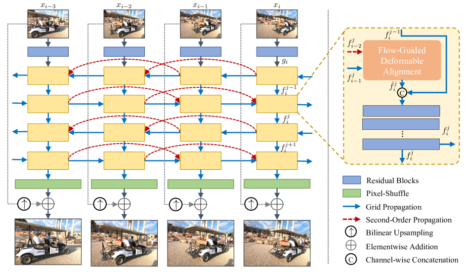
Grid Connections. Grid-like designs are seen in various vision tasks such as object detection [5, 30, 34], semantic segmentation [7, 30, 34, 43], and frame interpolation [25]. In general, these designs decompose a given image/feature into multiple resolutions, and grids are adopted across resolutions to capture both fine and coarse information. Unlike aforementioned methods, BasicVSR++ does not adopt a multi-scale design. Instead, the grid structure is designed for propagation across time in a bidirectional fashion. We link different frames with a grid connection to repeatedly refine the features, improving expressiveness.
Higher-Order Propagation. Higher-order propagation has been studied to improve gradient flow [16, 20, 28]. These methods demonstrate improvements in different tasks including classification [16] and language modeling [28]. However, these methods do not consider temporal alignment, which is shown critical in the task of VSR [2]. To allow temporal alignment in second-order propagation, we incorporate alignment into our propagation scheme by extending our flow-guided deformable alignment to the second-order settings.
Deformable Alignment. Several works [32, 33, 35, 37] employ deformable alignment. TDAN [32] performs alignment at the feature level using deformable convolution. EDVR [35] further proposes a Pyramid Cascading Deformable (PCD) alignment with a multi-scale design. Recently, Chan et al. [3] analyze deformable alignment and show that the performance gain over flow-based alignment comes from the offset diversity. Motivated by [3], we adopt deformable alignment but with a reformulation to overcome the training instability [3]. Our flow-guided deformable alignment is different from offset-fidelity loss [3]. The latter uses optical flow as a loss function during training. In contrast, we directly incorporate optical flow into our module as base offsets, allowing a more explicit guidance, both during training and inference.
3 Methodology
BasicVSR++ consists of two effective modifications for improving propagation and alignment. As shown in Fig. 2, given an input video, residual blocks are first applied to extract features from each frame. The features are then propagated under our second-order grid propagation scheme, where alignment is performed by our flow-guided deformable alignment. After propagation, the aggregated features are used to generate the output image through convolution and pixel-shuffling.
3.1 Second-Order Grid Propagation
Most existing methods adopt unidirectional propagation [12, 14, 27]. Several works [2, 10, 11] adopt bidirectional propagation for exploiting the information available in the video sequence. In particular, IconVSR [2] consists of a coupled propagation scheme with sequentially-connected branches to facilitate information exchange.
Motivated by the effectiveness of the bidirectional propagation, we devise a grid propagation scheme to enable repeated refinement through propagation. More specifically, the intermediate features are propagated backward and forward in time in an alternating manner. Through propagation, the information from different frames can be “revisited” and adopted for feature refinement. Compared to existing works that propagate features only once, grid propagation repeatedly extracts information from the entire sequence, improving feature expressiveness.
To further enhance the robustness of propagation, we relax the assumption of first-order Markov property in BasicVSR and adopt a second-order connection, realizing a second-order Markov chain. With this relaxation, information can be aggregated from different spatiotemporal locations, improving robustness and effectiveness in occluded and fine regions.
Integrating the above two components, we devise our second-order grid propagation as follows. Let be the input image, be the feature extracted from by multiple residual blocks, and be the feature computed at the -th timestep in the -th propagation branch. In this section, we describe the procedure for forward propagation, and the procedure for backward propagation is defined similarly.
To compute the feature , we first align and (following the second-order Markov chain) using our proposed flow-guided deformable alignment, which will be discussed in the next section:
| (1) |
where denote the optical flows from -th frame to the -th and -th frames, respectively, and represents flow-guided deformable alignment222.. The features are then concatenated and passed into a stack of residual blocks:
| (2) |
where , denotes the residual blocks, and denotes concatenation along channel dimension.
3.2 Flow-Guided Deformable Alignment
Deformable alignment [33, 35] has demonstrated significant improvements over flow-based alignment [9, 38] thanks to the offset diversity [3] intrinsically introduced in deformable convolution (DCN) [6, 42]. However, deformable alignment module can be difficult to train [3]. The training instability often results in offset overflow, deteriorating the final performance.
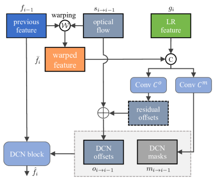
To take advantage of the offset diversity while overcoming the instability, we propose to employ optical flow to guide deformable alignment, motivated by the strong relation between deformable alignment and flow-based alignment [3]. The graphical illustration is shown in Fig. 3. In the rest of this section, we detail the alignment procedure for forward propagation. The procedure for backward propagation is defined similarly. The superscript is omitted for notational simplicity.
At the -th timestep, given the feature computed from the -th LR image, the feature computed for the previous timestep, and the optical flow to the previous frame, we first warp with :
| (3) |
where denotes the spatial warping operation. The pre-aligned features are then used to compute the DCN offsets and modulation masks . Instead of directly computing the DCN offsets, we compute the residue to the optical flow:
| (4) |
Here denotes a stack of convolutions, and denotes the sigmoid function. A DCN is then applied to the unwarped feature :
| (5) |
where denotes a deformable convolution.
The above formulation is designed only for aligning one single feature, and hence is not directly applicable to our second-order propagation. The most intuitive way to adapt to the second-order settings is to apply the above procedure to the two features, and , independently. However, this requires doubled computations, resulting in reduced efficiency. Furthermore, separate alignment potentially ignores the complementary information from the features. Therefore, we allow alignment of two features simultaneously. More specifically, we concatenate the warped features and flows to compute the offsets ():
| (6) |
A DCN is then applied to the unwarped features:
| (7) |
More details of the second-order flow-guided deformable alignment are provided in the supplementary material.
| BI degradation | BD degradation | |||||||
| Params (M) | Runtime (ms) | REDS4 [23] | Vimeo-90K-T [38] | Vid4 [21] | UDM10 [40] | Vimeo-90K-T [38] | Vid4 [21] | |
| Bicubic | - | - | 26.14/0.7292 | 31.32/0.8684 | 23.78/0.6347 | 28.47/0.8253 | 31.30/0.8687 | 21.80/0.5246 |
| VESPCN [1] | - | - | - | - | 25.35/0.7557 | - | - | - |
| SPMC [31] | - | - | - | - | 25.88/0.7752 | - | - | - |
| TOFlow [38] | - | - | 27.98/0.7990 | 33.08/0.9054 | 25.89/0.7651 | 36.26/0.9438 | 34.62/0.9212 | - |
| FRVSR [27] | 5.1 | 137 | - | - | - | 37.09/0.9522 | 35.64/0.9319 | 26.69/0.8103 |
| DUF [15] | 5.8 | 974 | 28.63/0.8251 | - | - | 38.48/0.9605 | 36.87/0.9447 | 27.38/0.8329 |
| RBPN [9] | 12.2 | 1507 | 30.09/0.8590 | 37.07/0.9435 | 27.12/0.8180 | 38.66/0.9596 | 37.20/0.9458 | - |
| EDVR-M [35] | 3.3 | 118 | 30.53/0.8699 | 37.09/0.9446 | 27.10/0.8186 | 39.40/0.9663 | 37.33/0.9484 | 27.45/0.8406 |
| EDVR [35] | 20.6 | 378 | 31.09/0.8800 | 37.61/0.9489 | 27.35/0.8264 | 39.89/0.9686 | 37.81/0.9523 | 27.85/0.8503 |
| PFNL [40] | 3.0 | 295 | 29.63/0.8502 | 36.14/0.9363 | 26.73/0.8029 | 38.74/0.9627 | - | 27.16/0.8355 |
| MuCAN [19] | - | - | 30.88/0.8750 | 37.32/0.9465 | - | - | - | - |
| TGA [13] | 5.8 | - | - | - | - | - | 37.59/0.9516 | 27.63/0.8423 |
| RLSP [8] | 4.2 | 49 | - | - | - | 38.48/0.9606 | 36.49/0.9403 | 27.48/0.8388 |
| RSDN [12] | 6.2 | 94 | - | - | - | 39.35/0.9653 | 37.23/0.9471 | 27.92/0.8505 |
| RRN [14] | 3.4 | 45 | - | - | - | 38.96/0.9644 | - | 27.69/0.8488 |
| BasicVSR [2] | 6.3 | 63 | 31.42/0.8909 | 37.18/0.9450 | 27.24/0.8251 | 39.96/0.9694 | 37.53/0.9498 | 27.96/0.8553 |
| IconVSR [2] | 8.7 | 70 | 31.67/0.8948 | 37.47/0.9476 | 27.39/0.8279 | 40.03/0.9694 | 37.84/0.9524 | 28.04/0.8570 |
| BasicVSR++ | 7.3 | 77 | 32.39/0.9069 | 37.79/0.9500 | 27.79/0.8400 | 40.72/0.9722 | 38.21/0.9550 | 29.04/0.8753 |
Discussion. Unlike existing methods [32, 33, 35, 37] that directly compute the DCN offsets, our proposed flow-guided deformable alignment adopts optical flow as guidance. The benefits are two-fold. First, since CNNs are known to have local receptive fields, the learning of offsets can be assisted by pre-aligning the features using optical flow. Second, by learning only the residue, the network needs to learn only small deviations from the optical flow, reducing the burden in typical deformable alignment modules. In addition, instead of directly concatenating the warped feature, the modulation masks in DCN act as attention maps to weigh the contributions of different pixels, providing additional flexibility.
4 Experiments
Two widely-used datasets are adopted for training: REDS [23] and Vimeo-90K [38]. For REDS, following BasicVSR [2], we use REDS4333Clips 000, 011, 015, 020 of REDS training set. as our test set and REDSval4444Clips 000, 001, 006, 017 of REDS validation set. as our validation set. The remaining clips are used for training. We use Vid4 [21], UDM10 [40], and Vimeo-90K-T [38] as test sets along with Vimeo-90K. All models are tested with downsampling using two degradations – Bicubic (BI) and Blur Downsampling (BD).
We adopt Adam optimizer [17] and Cosine Annealing scheme [22]. The initial learning rate of the main network and the flow network are set to and , respectively. The total number of iterations is 600K, and the weights of the flow network are fixed during the first 5,000 iterations. The batch size is 8 and the patch size of input LR frames is . We use Charbonnier loss [4] since it better handles outliers and improves the performance over the conventional -loss [18]. We use pre-trained SPyNet [26] as our flow network. Its parameters and runtime are considered inclusively in our method. The number of residual blocks for each branch is set to . The number of feature channels is . Detailed experimental settings and model architectures are provided in the supplementary material.


4.1 Comparisons with State-of-the-Art Methods
We conduct comprehensive experiments by comparing with 16 models, as listed in Table 1. The quantitative results are summarized in Table 1 and the speed and performance comparison is provided in Fig. 1(c). Note that the parameters reported above are inclusive of that in the optical flow network (if any). So the comparison is fair.
As shown in Table 1, BasicVSR++ achieves state-of-the-art performance on all datasets for both degradations. In particular, BasicVSR++ outperforms EDVR [35], a large-capacity sliding-window method, by up to 1.3 dB in PSNR, while having 65% fewer parameters. When compared to the previous state of the art, IconVSR [2], BasicVSR++ possesses fewer parameters but has improvements of up to 1 dB. As shown in Table 2, even if we train a lighter version of BasicVSR++ (denoted as BasicVSR++ (S)) with comparable network parameters and runtime to BasicVSR and IconVSR, our model still shows an improvement of 0.82 dB over BasicVSR and 0.57 dB over IconVSR. Such gains are considered significant in VSR.
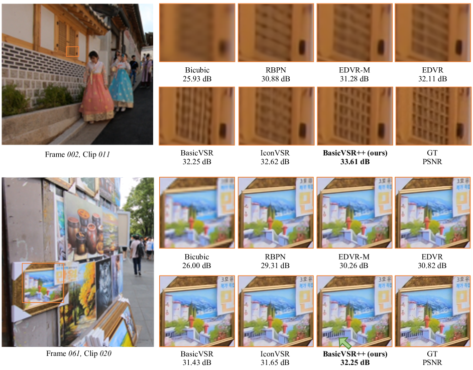
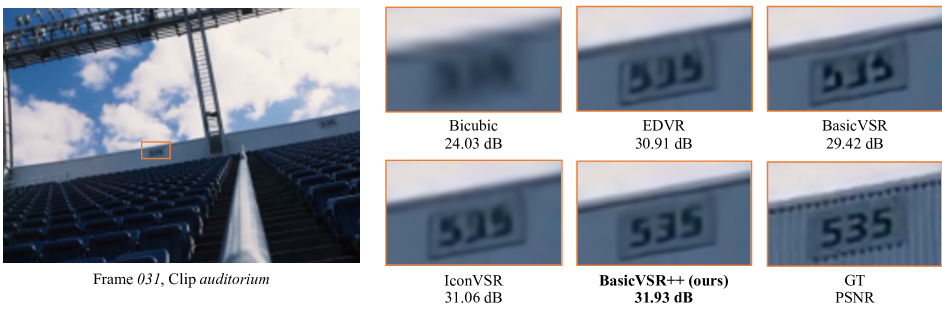
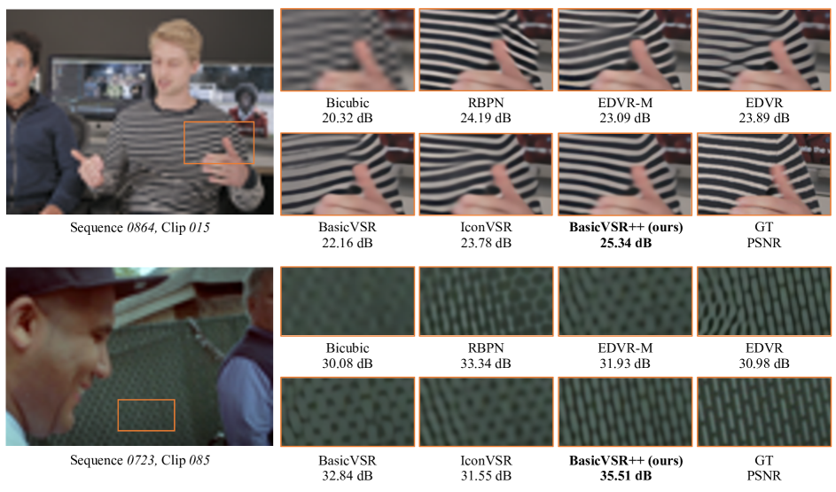
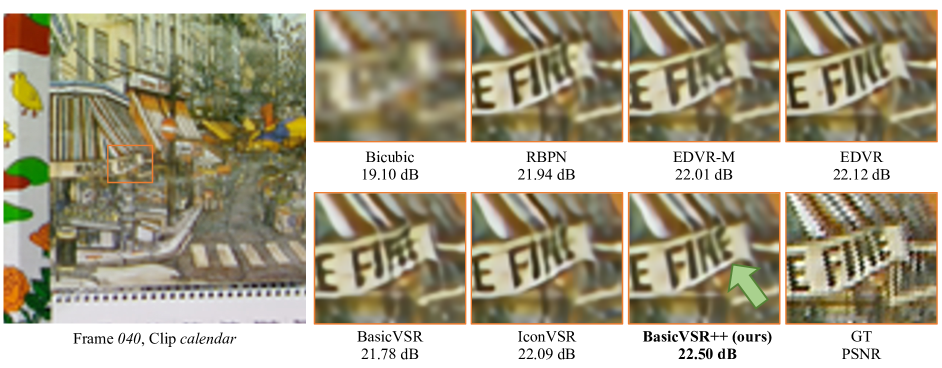
Some qualitative comparisons are shown in Fig. 11 to Fig. 14. BasicVSR++ successfully restores the fine details. In particular, BasicVSR++ is the only method that restores the wheel’s spokes in Fig. 11, the stairs in Fig. 13, and the building structure in Fig. 14. More examples are provided in the supplementary material.

5 Ablation Studies
To understand the contributions of the proposed components, we start with a baseline and gradually insert the components. From Table 3, it is apparent that each component brings considerable improvement, ranging from 0.14 dB to 0.46 dB in PSNR.
In theory, our proposed propagation schemes can be extended to higher orders and more propagation iterations. However, while the performance gain is considerable when increasing from first-order to second-order (i.e. (B)(C)), and from one to two iterations (i.e. (C)BasicVSR++), we observe in our preliminary experiments that further increasing the orders and number of iterations does not lead to a significant improvement ( dB in PSNR). Therefore, we keep both the orders and iterations to two.
| (A) | (B) | (C) | BasicVSR++ | |
| Flow-Guided Deform. Align. | ✓ | ✓ | ✓ | |
| Second-Order Propagation | ✓ | ✓ | ||
| Grid Propagation | ✓ | |||
| PSNR (dB) | 31.48 | 31.94 | 32.08 | 32.39 |
Second-Order Grid Propagation. We further provide some qualitative comparisons to understand the contributions of the proposed propagation scheme. As shown in the two examples of Fig. 7, the contribution of both the second-order propagation and grid propagation is more noticeable in regions that contain fine details and complex textures. In those regions, there is limited information from the current frame that can be employed for reconstruction. To improve the output quality of those regions, effective information aggregation from other video frames is necessary. With our second-order propagation scheme, the information can be transmitted via a robust and effective propagation. This complementary information essentially assists the restoration of the fine details. As shown in the examples, the network successfully restores the details with our components, whereas the counterparts without our components produce blurry outputs.
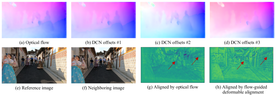
Flow-Guided Deformable Alignment. In Fig. 8(a-d), we compare the offsets with the optical flow computed by the flow estimation module in BasicVSR++. By learning only the residue to optical flow, the network produces offsets that are highly similar to the optical flow, but with observable differences. When compared to the baseline which aggregates information from only one spatial location indicated by the motion (optical flow), our proposed module allows retrieving information from multiple locations around, providing additional flexibility.
This flexibility leads to features with better quality, as shown in Fig. 8(g-h). When the warping is performed by using optical flow, the aligned features contain blurry edges, owing to the interpolation operation in spatial warping. In contrast, by gathering more information from the neighbors, the feature aligned by our proposed module is sharper and preserves more details.
To demonstrate the superiority of our designs, we compare our alignment module with two variants: (1) No optical flow is used. (2) Optical flow is used as in the offset-fidelity loss [3], i.e. the flow is merely used as supervision in the loss function (rather than serving as base offsets as in our method). As shown in Table 4, without using optical flow as guidance, the instability causes training to collapse, leading to a very poor PSNR value. When using the offset-fidelity loss, the training is stabilized. However, a drop of 2.17 dB from our full model is observed. Our flow-guided deformable alignment directly incorporates optical flow into the network to provide more explicit guidance, leading to better results.
| w/o Flow | Offset-Fidelity Loss [3] | Ours | |
| PSNR (dB) | 27.44 | 30.22 | 32.39 |
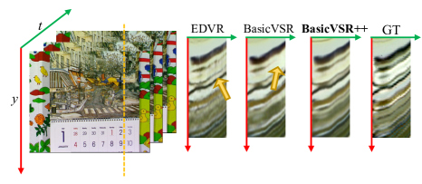
Temporal Consistency. Here, we examine the temporal consistency, which is another important direction in VSR. The recurrent framework intrinsically maintains a better temporal consistency in comparison to the sliding-window framework. In the sliding-window framework (e.g., EDVR [35]), each frame is reconstructed independently. In such a design, the consistency between the outputs cannot be guaranteed. In contrast, in the recurrent framework (e.g., BasicVSR [2]), the outputs are related through the propagation of the intermediate features. The temporal propagation essentially helps maintaining better temporal consistency.
In Fig. 9 we show a comparison of the temporal profiles between BasicVSR++ and two state-of-the-art methods – EDVR and BasicVSR. For the sliding-window method, the temporal profile from EDVR contains significant noise, indicating flickering artifacts in the output video. In contrast, for recurrent networks, without explicit modeling of temporal consistency, the profiles from BasicVSR and BasicVSR++ demonstrate better consistencies. However, the profile from BasicVSR still contains discontinuity. Benefit from our enhanced propagation and alignment, BasicVSR++ is able to aggregate richer information from the video frames, showing smoother temporal transition. The video results are given in the supplementary material.
6 NTIRE 2021 Challenge Results
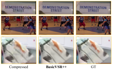
In NTIRE 2021, BasicVSR++ wins the video super-resolution track [29] with a compact and efficient structure. In addition to VSR, BasicVSR++ generalizes well to other restoration tasks. BasicVSR++ obtains two champions and one runner-up in the compressed video enhancement challenge [39]. Fig. 10 shows the restoration results of three different patches of compressed videos. BasicVSR++ successfully reduces the artifacts and produces outputs with much better qualities. The promising performance in the competitions demonstrate the generalizability and versatility of BasicVSR++.
7 Conclusion
In this work, we redesign BasicVSR with two novel components to enhance its propagation and alignment performance for the task of video super-resolution. Our model BasicVSR++ outperforms existing state of the arts by a large margin while maintaining efficiency. These designs generalizes well to other video restoration tasks including compressed video enhancement. These components are generic and we speculate that they will be useful for other video-based enhancement or restoration tasks such as deblurring and denoising.
References
- [1] Jose Caballero, Christian Ledig, Aitken Andrew, Acosta Alejandro, Johannes Totz, Zehan Wang, and Wenzhe Shi. Real-time video super-resolution with spatio-temporal networks and motion compensation. In CVPR, 2017.
- [2] Kelvin C.K. Chan, Xintao Wang, Ke Yu, Chao Dong, and Chen Change Loy. BasicVSR: The search for essential components in video super-resolution and beyond. In CVPR, 2021.
- [3] Kelvin C.K. Chan, Xintao Wang, Ke Yu, Chao Dong, and Chen Change Loy. Understanding deformable alignment in video super-resolution. In AAAI, 2021.
- [4] Pierre Charbonnier, Laure Blanc-Feraud, Gilles Aubert, and Michel Barlaud. Two deterministic half-quadratic regularization algorithms for computed imaging. In ICIP, 1994.
- [5] Kai Chen, Jiaqi Wang, Shuo Yang, Xingcheng Zhang, Yuanjun Xiong, Chen Change Loy, and Dahua Lin. Optimizing video object detection via a scale-time lattice. In CVPR, 2018.
- [6] Jifeng Dai, Haozhi Qi, Yuwen Xiong, Yi Li, Guodong Zhang, Han Hu, and Yichen Wei. Deformable convolutional networks. In ICCV, 2017.
- [7] Damien Fourure, Rémi Emonet, Élisa Fromont, Damien Muselet, Alain Trémeau, and Christian Wolf. Residual conv-deconv grid network for semantic segmentation. In BMVC, 2017.
- [8] Dario Fuoli, Shuhang Gu, and Radu Timofte. Efficient video super-resolution through recurrent latent space propagation. In ICCVW, 2019.
- [9] Muhammad Haris, Greg Shakhnarovich, and Norimichi Ukita. Recurrent back-projection network for video super-resolution. In CVPR, 2019.
- [10] Yan Huang, Wei Wang, and Liang Wang. Bidirectional recurrent convolutional networks for multi-frame super-resolution. In NIPS, 2015.
- [11] Yan Huang, Wei Wang, and Liang Wang. Video super-resolution via bidirectional recurrent convolutional networks. TPAMI, 2018.
- [12] Takashi Isobe, Xu Jia, Shuhang Gu, Songjiang Li, Shengjin Wang, and Qi Tian. Video super-resolution with recurrent structure-detail network. In ECCV, 2020.
- [13] Takashi Isobe, Songjiang Li, Xu Jia, Shanxin Yuan, Gregory Slabaugh, Chunjing Xu, Ya-Li Li, Shengjin Wang, and Qi Tian. Video super-resolution with temporal group attention. In CVPR, 2020.
- [14] Takashi Isobe, Fang Zhu, and Shengjin Wang. Revisiting temporal modeling for video super-resolution. In BMVC, 2020.
- [15] Younghyun Jo, Seoung Wug Oh, Jaeyeon Kang, and Seon Joo Kim. Deep video super-resolution network using dynamic upsampling filters without explicit motion compensation. In CVPR, 2018.
- [16] Nan Rosemary Ke, Anirudh Goyal, Olexa Bilaniuk, Jonathan Binas, Michael C Mozer, Chris Pal, and Yoshua Bengio. Sparse attentive backtracking: Temporal creditassignment through reminding. In NIPS, 2018.
- [17] Diederik Kingma and Jimmy Ba. Adam: A method for stochastic optimization. In ICLR, 2015.
- [18] Wei-Sheng Lai, Jia-Bin Huang, Narendra Ahuja, and Ming-Hsuan Yang. Deep laplacian pyramid networks for fast and accurate super-resolution. In CVPR, 2017.
- [19] Wenbo Li, Xin Tao, Taian Guo, Lu Qi, Jiangbo Lu, and Jiaya Jia. MuCAN: Multi-correspondence aggregation network for video super-resolution. In ECCV, 2020.
- [20] Tsungnan Lin, Bill G Horne, Peter Tino, and C Lee Giles. Learning long-term dependencies in NARX recurrent neural networks. IEEE Transactions on Neural Networks, 1996.
- [21] Ce Liu and Deqing Sun. On bayesian adaptive video super resolution. TPAMI, 2014.
- [22] Ilya Loshchilov and Frank Hutter. SGDR: Stochastic gradient descent with warm restarts. arXiv preprint arXiv:1608.03983, 2016.
- [23] Seungjun Nah, Sungyong Baik, Seokil Hong, Gyeongsik Moon, Sanghyun Son, Radu Timofte, and Kyoung Mu Lee. NTIRE 2019 challenge on video deblurring and super-resolution: Dataset and study. In CVPRW, 2019.
- [24] Seungjun Nah, Sanghyun Son, and Kyoung Mu Lee. Recurrent neural networks with intra-frame iterations for video deblurring. In CVPR, 2019.
- [25] Simon Niklaus and Feng Liu. Softmax splatting for video frame interpolation. In CVPR, 2020.
- [26] Anurag Ranjan and Michael J Black. Optical flow estimation using a spatial pyramid network. In CVPR, 2017.
- [27] Mehdi S M Sajjadi, Raviteja Vemulapalli, and Matthew Brown. Frame-recurrent video super-resolution. In CVPR, 2018.
- [28] Rohollah Soltani and Hui Jiang. Higher order recurrent neural networks. arXiv preprint arXiv:1605.00064, 2016.
- [29] Sanghyun Son, Suyoung Lee, Seungjun Nah, Radu Timofte, Kyoung Mu Lee, Kelvin C.K. Chan, et al. NTIRE 2021 challenge on video super-resolution. In CVPRW, 2021.
- [30] Ke Sun, Yang Zhao, Borui Jiang, Tianheng Cheng, Bin Xiao, Dong Liu, Yadong Mu, Xinggang Wang, Wenyu Liu, and Jingdong Wang. High-resolution representations for labeling pixels and regions. arXiv preprint arXiv:1904.04514, 2019.
- [31] Xin Tao, Hongyun Gao, Renjie Liao, Jue Wang, and Jiaya Jia. Detail-revealing deep video super-resolution. In CVPR, 2017.
- [32] Yapeng Tian, Yulun Zhang, Yun Fu, and Chenliang Xu. TDAN: Temporally deformable alignment network for video super-resolution. In CVPR, 2018.
- [33] Hua Wang, Dewei Su, Longcun Jin, and Chuangchuang Liu. Deformable non-local network for video super-resolution. IEEE Access, 2019.
- [34] Jingdong Wang, Ke Sun, Tianheng Cheng, Borui Jiang, Chaorui Deng, Yang Zhao, Dong Liu, Yadong Mu, Mingkui Tan, Xinggang Wang, Wenyu Liu, and Bin Xiao. Deep high-resolution representation learning for visual recognition. TPAMI, 2020.
- [35] Xintao Wang, Kelvin C.K. Chan, Ke Yu, Chao Dong, and Chen Change Loy. EDVR: Video restoration with enhanced deformable convolutional networks. In CVPRW, 2019.
- [36] Xiaoyu Xiang, Yapeng Tian, Yulun Zhang, Yun Fu, Jan P Allebach, and Chenliang Xu. Zooming Slow-Mo: Fast and accurate one-stage space-time video super-resolution. In CVPR, 2020.
- [37] Xiangyu Xu, Muchen Li, Wenxiu Sun, and Ming-Hsuan Yang. Learning spatial and spatio-temporal pixel aggregations for image and video denoising. TIP, 2020.
- [38] Tianfan Xue, Baian Chen, Jiajun Wu, Donglai Wei, and William T Freeman. Video enhancement with task-oriented flow. IJCV, 2019.
- [39] Ren Yang, Radu Timofte, Jing Liu, Yi Xu, Xinjian Zhang, Minyi Zhao, Shuigeng Zhou, Kelvin CK Chan, Shangchen Zhou, Xiangyu Xu, et al. NTIRE 2021 challenge on quality enhancement of compressed video: Methods and results. In CVPRW, 2021.
- [40] Peng Yi, Zhongyuan Wang, Kui Jiang, Junjun Jiang, and Jiayi Ma. Progressive fusion video super-resolution network via exploiting non-local spatio-temporal correlations. In ICCV, 2019.
- [41] Shangchen Zhou, Jiawei Zhang, Jinshan Pan, Haozhe Xie, Wangmeng Zuo, and Jimmy Ren. Spatio-temporal filter adaptive network for video deblurring. In ICCV, 2019.
- [42] Xizhou Zhu, Han Hu, Stephen Lin, and Jifeng Dai. Deformable ConvNets v2: More deformable, better results. In CVPR, 2019.
- [43] Juntang Zhuang, Junlin Yang, Lin Gu, and Nicha Dvornek. ShelfNet for fast semantic segmentation. In ICCVW, 2019.
Appendix A Network Architecture
We use pretrained SPyNet [26] as our flow network. The number of residual blocks for the initial feature extraction is set to , and the number of residual blocks for each propagation branch is set to . The feature channel is set to .
The architecture of our second-order deformable alignment is highly similar to the first-order counterpart (Fig. 3 in the main paper). The only difference is that the pre-aligned features and optical flows from different timesteps are concatenated, and passed to the offset estimation module and mask estimation module . Their architectures are detailed in Table 5. We set the DCN kernel size to and the number of deformable groups to . Codes will be released.
Appendix B Experimental Settings
Datasets. Two widely-used datasets are adopted for training: REDS [23] and Vimeo-90K [38]. For REDS, following BasicVSR [2], we use REDS4555Clips 000, 011, 015, 020 of REDS training set. as our test set and REDSval4666Clips 000, 001, 006, 017 of REDS validation set. as our validation set. The remaining clips are used for training. We use Vid4 [21], UDM10 [40], and Vimeo-90K-T [38] as test sets along with Vimeo-90K.
Degradations. All models are tested with downsampling using two degradations – Bicubic (BI) and Blur Downsampling (BD). For BI, the MATLAB function imresize is used for downsampling. For BD, we blur the ground-truth by a Gaussian filter with , followed by a subsampling every four pixels.
Training Settings. We adopt Adam optimizer [17] and Cosine Annealing scheme [22]. When trained on REDS, the initial learning rate of the main network and the flow network are set to and , respectively. The total number of iterations is 600K, and the weights of the flow network are fixed during the first 5,000 iterations. The batch size is 8 and the patch size of input LR frames is . We use Charbonnier loss [4] since it better handles outliers and improves the performance over the conventional -loss [18]. During training, LR frames are used as inputs. Since Vimeo-90K contains only seven frames per sequence, networks trained solely on Vimeo-90K may not be able to capture long-term dependencies. Therefore, we initialize the model using the weights trained on REDS when trained on Vimeo-90K. The number of finetune iterations is 300K.
Test Settings. We take the full video sequence as inputs to explore information from all video frames for restoration.
| Layer | ||
|---|---|---|
| 1. | conv(196, 64, 3) | |
| 2. | LeakyReLU(0.1) | |
| 3. | conv(64, 64, 3) | |
| 4. | LeakyReLU(0.1) | |
| 5. | conv(64, 64, 3) | |
| 6. | LeakyReLU(0.1) | |
| 7. | conv(64, 288, 3) | conv(64, 144, 3) |
Appendix C Qualitative Comparisons
In this section, we provide additional qualitative comparisons on REDS4 [23], UDM10 [40], Vimeo-90K [38], and Vid4 [21]. From the examples, we see that BasicVSR++ is able to restore the fine details, leading to plausible results. A video demo is also provided in the submitted zip file.
