Identifying tax evasion in Mexico with tools from network science and machine learning

Abstract

Mexico has kept electronic records of all taxable transactions since 2014. Anonymized data collected by the Mexican federal government comprises more than 80 million contributors (individuals and companies) and almost 7 billion monthly-aggregations of invoices among contributors between January 2015 and December 2018. This data includes a list of almost ten thousand contributors already identified as tax evaders, due to their activities fabricating invoices for non-existing products or services so that recipients can evade taxes. Harnessing this extensive dataset, we build monthly and yearly temporal networks where nodes are contributors and directed links are invoices produced in a given time slice. Exploring the properties of the network neighborhoods around tax evaders, we show that their interaction patterns differ from those of the majority of contributors. In particular, invoicing loops between tax evaders and their clients are over-represented. With this insight, we use two machine-learning methods to classify other contributors as suspects of tax evasion: deep neural networks and random forests. We train each method with a portion of the tax evader list and test it with the rest, obtaining more than 0.9 accuracy with both methods. By using the complete dataset of contributors, each method classifies more than 100 thousand suspects of tax evasion, with more than 40 thousand suspects classified by both methods. We further reduce the number of suspects by focusing on those with a short network distance from known tax evaders. We thus obtain a list of highly suspicious contributors sorted by the amount of evaded tax, valuable information for the authorities to further investigate illegal tax activity in Mexico. With our methods, we estimate previously undetected tax evasion in the order of $10 billion USD per year by about 10 thousand contributors.

1 Introduction

Tax has a crucial role in the economic growth and welfare of the general population. Paid taxes allow for government spending and public expenditures (in the short, medium, and long terms) such as education, healthcare, housing, pensions, security, and infrastructure CPEUM . Tax collection in Mexico is determined by a series of laws (Ley de Ingresos de la Federación, in Spanish) specifying the eligibility of taxpayers, tax rates and types, as well as the periodicity of fees and means of payment.

Despite the general view that taxes are justified since they allow the Mexican state to fund beneficial activities for society, some individuals, corporations, or trusts may decide to illegally evade taxes by misrepresenting their state of affairs to the Tax Administration Service in Mexico (Servicio de Administración Tributaria, or SAT). In this sense, tax evasion is the reduction of constitutional tax liability by dishonest reporting, such as understating financial gains or overstating deductions tovar2000evasion .

Since 2014, Mexico has kept electronic records of all taxable transactions by means of a digital receipt or invoice known as Comprobante Fiscal Digital por Internet (CFDI). Each of these mandatory receipts includes data on the product or service transferred between taxpayers, date of transaction, cost, and corresponding tax amount. CFDIs are XML documents with technical specifications updated annually by SAT, including a certification seal that can only be produced by authorized parties CFDISAP . Since CFDIs potentially uncover networks of individuals and legal entities involved in commercial transactions leading to tax revenue, they are an integral part of formal investigations by SAT in tax evasion, money laundering, and other tax-related illegal activities.

Among all forms of tax evasion, here we focus in situations where taxpayers issue CFDIs in the absence of actual economic activity to increase tax deductions. Such legal entities, known as ‘enterprises billing simulated operations’ (‘empresas que facturan operaciones simuladas’, or EFOS), are typically characterized by a lack of employees or infrastructure, as well as a fake or constantly changing address used to avoid detection. As a result of investigations already led by SAT, EFOS can be classified as definitive or alleged tax evaders DefEFO . In order to operate, EFOS require the participation of ‘enterprises deducting simulated operations’ (‘empresas que deducen operaciones simuladas’, or EDOS). Even if EDOS engage in illegal activity alongside EFOS, they tend to have demonstrable stability in their workforce, assets, and tax contributions. By receiving CFDIs associated with simulated operations, EDOS aim to reduce their tax rate to avoid payments to SAT and eventually obtain further fiscal benefits.

In order to decrease the risk of systematic tax evasion, the Mexican federal government has established fiscal law (known as ‘Código Fiscal de la Federación’) describing the official procedure to identify taxpayers as EFOS: a) First, SAT determines the lack of actual economic activity behind a set of CFDIs. b) Then, the government notifies the relevant legal entities via its official publication (‘Diario Oficial de la Federación’). c) Alleged EFOS have 15 days to contest the claim. d) Associated EDOS (that have received the suspicious CFDIs) can correct their standing with SAT by resubmitting appropriate tax forms. e) Finally, if any tax revenue has been lost to illegal activity, SAT classifies relevant taxpayers as definitive EFOS and specifies the type of crime following fiscal law. Definitive EFOS are unable to emit further CFDIs.

Despite its effectiveness, the official procedure of detecting tax evasion is time and resource consuming, particularly in initial stages of the process where suspicious CFDIs and alleged EFOS need to be manually selected from millions of contributors and billions of transactions each year. In order to complement these efforts, automated computational and statistical techniques (with tools from network science and machine learning) can be used to characterize the network of issued/received CFDIs between definitive EFOS and other taxpayers. By analyzing the temporal properties of the network of all taxable transactions in Mexico from 2015 to 2018, here we show evidence of a group of highly suspicious contributors with behavior statistically similar to that of definitive EFOS, as well as estimates of previously undetected tax evasion. When combined with current practices at SAT, this information has the potential to increase the efficacy of the governmental response to illegal tax activity in Mexico.

2 Data

Taxpayers in Mexico are identified by their tax number (‘Registro Federal de Contribuyentes’, or RFC), a unique string of alphanumerical characters used to emit and receive invoices, submit tax statements and engage in other procedures. Since 2014, a large number of income and outcome transactions between taxpayers in Mexico have been recorded in CFDIs and stored by SAT.

The data used in this work includes:

• A set of 81,511,015 taxpayer identifiers, anonymized to protect individual identities, which we denote RFCAs, and categorical information for each one of them that includes: taxpayer type (individual or legal entity), location, date of registration, and economical sector and activity.

• A total of 6,823,415,757 monthly CFDI aggregated emissions between taxpayers distributed between January 2015 and December 2018, which include the RFCA of both the emitter and receiver of the transaction, the month and year, type (either income or outcome), the number of transactions for that month, and the total amounts associated with them.

• A list of 8,570 RFCAs previously identified by Mexican government authorities as definitive or alleged EFOS. We use this data to train machine learning models and as focal points in the network science approach.

In the 48 months of CFDI emissions we analyze, 7,571,093 RFCAs emitted at least one CFDI, so that the already identified evaders (EFOS) account only for 0.0072% of active taxpayers (those who at least emitted one receipt during the period of study). This means that the data is highly unbalanced: the ratio between the identified class (EFOS) and the undetermined ones is quite different, which has an impact in the design of the models and approaches we use.

In what follows, when we refer to a RFCA as an EFOS, we mean those taxpayers already identified by the authorities as either definitive or alleged evaders. Unclassified RFCAs correspond to those that have not been classified as EFOS by the authorities, and we refer as suspects to those RFCA which are classified as possible evaders by our methods.

3 Results

3.1 Deep Neural Networks

As a first classification method of unknown RFCs on whether they behave similarly (or not) to definitive EFOS, we implement an artificial neural network (ANN). ANNs are models of automatic learning inspired by the human brain. They consist of a collection of interconnected mathematical functions with characteristics analogous to those of biological neurons and are thus called neurons. Just like biological neurons, an artificial neuron collects and classifies information based on its input connections with other neurons, and thereby alternates between an active and inactive state. The connections between neurons have a weight associated with them representative of the intensity of the interaction, such that highly weighted connections are more relevant than those associated with a low weight to modify their activation state. It is via modification of the connections weight between neurons that a neural network learns to identify patterns, a process referred to as training.

Neurons of an artificial neural network are often divided into different layers: an input layer that receives the data for classification; hidden layers that undertake the classification process through modification of the weights among neurons and adjustment of the input of data weights until the classification undertaken by the network is optimal; and an output layer, from which the final result of the networks’ classification of input data is derived. The output of the network is compared with the desired outcome via a loss function that yields an error quantifier. During training, these errors are propagated through the network to update the weights and minimize the loss function. ANNs have been used in a variety of tasks, including computer vision hongtao2016applications , voice recognition venayagamoorthy1998voice , automatic translation zhang2015deep , board and video games tesauro1988neural ; clark2015training ; NeuralState and medical diagnostics amato2013artificial . They have also been used in a variety of applications in financial services, from forecasting to market studies kimoto1990stock ; mizuno1998application ; wilson1994bankruptcy , to fraud detection CreditCardFraud and risk assessment trippi1992neural ; yu2008credit . A neural network can evaluate price data and discover opportunities to make commercial decisions based on data analysis. Networks can distinguish subtle, non-linear inter-dependencies and patterns that other methods of technical analysis cannot.

Data preparation

In our implementation, we design an ANN that receives input data from all CFDIs associated with an issuing RFCA. By means of a technique referred to as re-sampling japkowicz2000class , we form a balanced sample of unknown RFCAs and definitive EFOS. The re-sampling method considered in this implementation is comprised of random re-sampling of the small class (CFDIs issued by definitive EFOS) until it contains as many examples as the other class, in order to finally obtain a large dataset with the same quantity of CFDIs issued by unknown RFCAs and definitive EFOS.

The model associates each RFCA with a value between 0 and 1 related to the probability that it will be an EFOS. In what follows, we describe the procedure used to design, train and evaluate the ANN. We will follow by presenting some results and conclusions.

Modeling

ANN design

A dynamic recurrent neuronal network (DRNN) is a special type of neural network that allows introduction of an arbitrary number of rows of data (input variables) at the same time, which is useful in this context since RFCAs have varying amounts of issued CFDIs. Recurrent neural networks are structures in which the output of each execution step provide the input to the following step; this enables them to retain learned information over time. Long short term memory (LSTM) describes the design of artificial neurons, i.e., those that give memory to the ANN. These neurons have the best known performance to date and are particularly effective for datasets derived from time series greff2016lstm ; yin2017comparative ; chung2014empirical . In particular, out of several structures tested, the best performance was obtained with an DRNN with three LSTM cell layers, each with 256 neurons, using a hyperbolic tangential function to calculate their internal state.

It is worth noting that the connections of an DRNN are not only among different layers, but are also connections from a neuron to itself over time. This means that the error propagation for weight adjustment occurs, not only among different nodes, but also between the same node and different time steps, as shown in Fig. 1.

Figure 1: One part of neural network $A$ observes an input $x_{t}$ and calculates a value $h_{t}$. The cycle allows information to flow from one step of the network to the next. If we unroll the cycle, one recurrent neural network can be considered as multiple copies of the same network, such that each one passes a message to a successor.

An LSTM cell is controlled by three gates: the Forget gate, the Input gate and the Output gate. Each gate within the cell is a different neural network that decides what information is allowed in the cell’s state, and which functions as the network’s memory. The gates can learn what information is relevant to save or forget during the exercise. The Forget gate controls the amount of information that will be stored in the memory and discards irrelevant information. The Input gate controls the amount of new input that will be stored in the memory, i.e., determines the importance of new information. Finally, the Output gateway determines the characteristics of the analyzed information to obtain an output that will allow correct classification.

The architecture of the neuronal network used to classify RFCA as possible EFOS is made up of three hidden LSTM cell layers each with 256 neurons connecting each neuron in a layer to a neuron in the following layer. The network unrolls over time to analyze all the invoices issued by an RFCA and, from what has been analyzed, classifies it into EFOS or non-EFOS.

ANN training

The training of the ANN is carried out from the following steps. All the RFCAs previously identified as definitive EFOS are divided into two sets, one with $2,981$ of the RFCAs, referred to as training set, and another one with $745$ EFOS, the so-called test set. The same quantity of unknown RFCAs is added to the test set. One million unknown RFCAs are added to the training set and then the $2,981$ definitive EFOS are added until we obtain the same quantity of unknown RFCAs, ending up with a set of $2,000,000$ RFCAs. Thus, both sets will be made up of 50% of the data from definitive EFOS, corresponding to the randomly selected EFOS income-type CFDI records, and 50% of the unknown RFCAs randomly selected from the total population. Data of the associated CFDI is obtained for each RFCA. These are the data that are supplied to the ANN and from which the ANN is trained by adjusting internal parameters. Following the training process, the ANN is presented the set of test data that it has never seen previously, to evaluate its performance.

Additional variables considered

In addition to incorporating the quantitative variables mentioned in section 2, we attempted to incorporate categorical data such as the type and situation of the contributor, the situation-description, the status of the contributor, the start date of operations, the sector and federal entity. We also considered incorporating data related to interactive networks (see section 3.3), such as the degree of output and input, betweenness, closeness, stress, radiality and page rank. However, all the ANN trained with these variables performed equally or worse than the ANN that only used CFDI data.

Performance evaluation

We used the F1-score Rijsbergen:1979:IR as a measure to evaluate the competence of the trained model. The F1-score is obtained by calculating the precision harmonic mean and the recall. Precision is the proportion of relevant instances correctly classified out of all the instances that the model believes are relevant. If TP are the true positives and FP the false positives, precision would be given by $\textrm{TP}/(\textrm{TP}+\textrm{FP})$ (see Table 1). Precision answers the question: How many of the selected RFCAs are actually EFOS? Recall is the proportion of the incorrectly classified relevant instances out of all the actually relevant instances, $\textrm{TP}/(\textrm{TP}+\textrm{FN})$, where FN are the false negatives, that answers the question of all RFCAs that are actually EFOS: How many were correctly classified? The harmonic mean is defined as the value obtained when the number of values in the dataset is divided by the sum of its reciprocals. It is a type of mean generally used for numbers that represent a ratio or proportion (like the precision and recall) as it equalizes the weight of each datapoint. An F1-score attains its best value at 1 (perfect precision and recall) and the worst at 0. Table 1 shows a way of separating the classifications made by the neuronal network to allow their evaluation.

	Predicted class
		P	N
Real class	P	True positives (TP)	False negatives (FN)
	N	False positives (FP)	True negatives (TN)

Table 1: Confusion matrix for binary classification. The true positives (TP) are the examples that the model correctly classified as EFOS. The false negatives (FN) are the examples that the model classified as non-EFOS, but that are actually EFOS. The true negatives (TN) are examples that the model classified as non-EFOS and have not been previously classified as EFOS. The false positives (FP) are examples that the model classified as EFOS, but that were not previously detected as such

For example, if we take 500 definitive EFOS and 500 unknown ones, and we feed them to our network, we find that $\textrm{TP}=448$, $\textrm{FN}=52$, $\textrm{TN}=416$ and $\textrm{FP}=84$. Therefore the precision was $0.845$, the recall was $0.896$, and we obtained an F1-score of $0.87$. If we make the calculation with 1000 alleged EFOS, we obtain $TP=881$, $FN=119$ ($TN=FP=0$ by definition), so the precision is 1, while the recall is $0.881$. We thus obtain an F1-score of 0.94.

The RFCAs in the set of “alleged” show the same behavior that the model indentified by training with the set of “definitive”, and it ends up identifying 88% as EFOS.

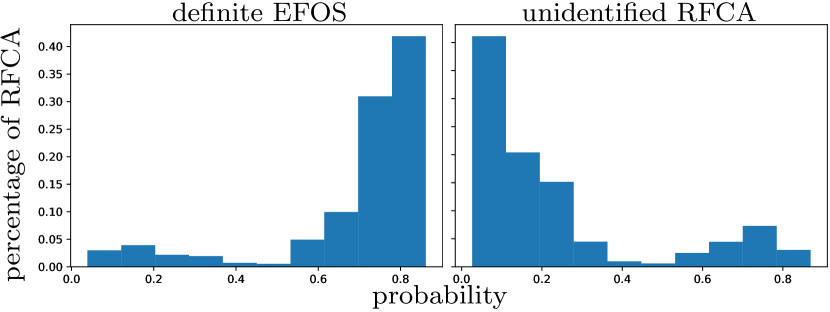
In Figure 2 we observe that the model is sure of its decision most of the time (i.e. ends with a very high or very low probability, with a bimodal distribution). Additionally, in the probability distribution of the non-identified RFCAs, there is a percentage that the model is classifying with high probability (i.e., the model is sure that they are EFOS) but has not previously classified them as EFOS.

Figure 2: Histograms of the probabilities assigned by the neural network to different sets of RFCAs. (left) We observe that the network correctly assigns most of them a high probability of being EFOS. (right) We observe a bimodal distribution in which there is a considerable percentage of RFCAs that are assigned a high probability of being EFOS.

One of the greatest challenges in neural networks is to interpret what the network is learning from the data. It is not only important to develop a solid solution with great predictive power; it is also of interest to understand the functioning of the developed model, i.e., which variables are the most relevant, the presence of correlations, possible causal relationships, etc. To deepen our understanding of the results, we applied two techniques to determine the more relevant variables that we detail below.

The first technique is based on hypothetical analysis or simulation, and is used to measure the relative influence of the input variables on the model results. In particular, to measure the importance of the variables, we took a sample of our data $X$ and calculated the model predictions once $Y$ is trained. Then, for each variable $x_{i}$ we cause a perturbation of this variable (and only this variable) via a normal random distribution centered on 0 with a scale 20% of the variable mean, and calculate the prediction $Y_{i}$. We measure the effect exerted by this perturbation by calculating the difference of the quadratic root mean between the original output $Y$ and the perturbed $Y_{i}$. A larger mean square root difference means that the variable is “more important”. Table 2 (left) shows the five variables of greatest importance for the neuronal network.

The second technique consists of the analysis of principal components, a statistical technique to convert high-dimensional to low dimensional data by selecting the most important characteristics that capture most of the information about the dataset. Characteristics are selected as a function of the variation they cause on the output. The characteristic that causes the highest variance is the first component, the characteristic responsible for the second highest variance is considered the second principal component, and so on. It is important to mention that the principal components are not correlated with each other. The importance of each variable is reflected in the magnitude of the corresponding values in vectors that characterize a linear transformation (greater magnitude indicates greater importance). Table 2 (right) lists the five variables that best characterize the dataset based on the first principal component, which contributes 99% of the variance. The variable magnitudes are normalized so that the sum of squares is equal to 1.

Variable	Perturbation effect
Sub-active	0.2099
Active total	0.1813
Total amount after active	0.1419
IVA after active	0.1083
Cancelled amount	0.0748

Variable	Magnitude
Active total	0.74925125
Sub-active	0.64598303
Total amount after active	0.10326791
IVA after active	0.1032678
Cancelled amount	0.0000125

Table 2: (left) Effect of the perturbation on the probability assigned by the neural network; (right) importance of the variables based on the absolute value of the magnitude of the first principal component used to characterize the dataset.

Model results

The ANN efficiently classifies the identified EFOS that it has been presented with, and using the trained model, we classify as “suspicious” the unknown RFCAs to which the ANN assigns a greater probability of behaving similarly to published EFOS. The ANN classified $149,921$ unknown RFCAs, corresponding to 1.98% of the total, as suspicious, using the threshold probability ($>0.8$).

3.2 Random Forest

As a second method of classification, we use the automatic technique named Random Forest (RF). Techniques of automatic classification, including RF, detect groups of elements with similar statistical patterns in an available dataset, and from the knowledge acquired, make decisions about the membership of new elements in these groups. In our case, we consider the characteristics of EFOS published by SAT and we compare them to unknown RFCAs.

A RF is constructed by randomly combining different decision trees in order to obtain results robust to noise sources inherent to the algorithm. A decision tree is a mathematical algorithm made up of a set of questions ordered and connected to each other through their responses (i.e., the formulation of a question depends on the answer to a preceding question). These questions involve the variables or characteristics of the data utilized. In constructing a decision tree each node represents one of the questions and each fork depends on its answer. Thus, in finishing the construction of a decision tree we can follow a path determined by questions and answers, finally answering the main question: how likely is this RFCA to be an EFOS?

In statistical models like RF it is necessary to maintain a balance between measures such as the variance (variability in the prediction of models for different elements) and bias (the difference between actual and predicted value). To achieve this balance, an effective technique is the combination of various models, e.g., the combination of decision trees to form a RF. In this way, each decision tree issues a classification (i.e., a probability of suspecting it is an EFOS associated to a RFCA) and the final result of the RF is the most probable classification among all the trees constructed. One of the tasks to resolve in constructing a RF is to find the optimum number of decision trees used to determine the combination that generates the final solution.

In our case, the RF technique is considered adequate since it offers the following advantages:

• Data preparation is minimal. It is only necessary to rely on a dataset where each element to classify, in this case each RFCA, is unique and has a fixed number of characteristics associated with each one of the classes involved, in this case definitive or unknown.

• It can handle a large number of variables without discriminating any one of them.

• It has been demonstrated that it is one of the methods with highest precision among the classification algorithms breiman2001random .

• It performs well with large-volume databases (which applies to the present case study) The result of the RF is a number between 0 and 1 for each evaluated RFCA, which will be interpreted as the probability that each unknown RFCA is a potential EFOS.

Data preparation

For the implementation of the RF algorithm, the information by issuer is initially grouped, since this analysis is focused on classification of issuing RFCAs. As a result, a unique record for each issuing RFCA is obtained for each of the 48 months considered.

Subsequently, by means of a technique called undersampling liu2008exploratory a balanced sample of unknown RFCA and definitive EFOS is generated. This technique seeks to determine the optimal number of RFCAs that will allow obtaining a balanced sample of the data (i.e., has the same quantity of unknowns and definitives) as well as a representative one (i.e., that will capture the characteristics of the whole population with the number of RFCAs selected. This process yields a sample with 1561 definitive EFOS and 1561 unknown RFCAs. The sample obtained so far is the baseline dataset used for implementation of the RF algorithm.

As part of the data preparation phase, two independent treatments are applied to the previously generated sample:

1. The data were analyzed to determine what type of data transformation is viable for each of the sample variables. The family of box cox transformations was used to improve the normality of the data and equalize the variance in order to improve the algorithm’s performance osborne2010improving .

2. Principal components analysis (PCA) was used. This consists in reduction of the dimensionality of the dataset by unifying existing variables to create new ones. This method is recommended to improve the performance of the algorithms in question wold1987principal .

Model construction

Using the RF algorithm three models were constructed that correspond to the following scenarios and use the sample generated in the previous section:

• First scenario: implementation of the RF algorithm without transformation

• Second scenario: implementation of the RF algorithm using the data sample to which PCA was applied.

• Third scenario: implementation of the RF algorithm using the data sample to which the box cox transformation was applied.

For each of the above scenarios, training of the RF algorithm aims to find the optimum number of constituent decision trees. This is achieved by performing iterations of the algorithm, modifying the number of trees used, and determining when the error generated stabilizes at a minimum value. It was concluded that the optimal number of decision tress was 100.

Performance evaluation

The following measures were used to evaluate the above scenarios:

• Receiver operating characteristic (ROC) curve: is a performance measure with values between 0 and 1; the higher the value, the better the performance is considered. An ROC curve is constructed using the information from two characteristics: the sensitivity (possibility of appropriately classifying a positive individual, in this case a definitive EFOS) and the specificity (possibility of appropriately classifying a negative individual, in this case an unknown RFCA that is not actually a definitive RFCA) martinez2003curva .

• Error: is a penalty measure. The closer it is to 0, the better it is considered. The error quantifies the part of the model that is making a mistake in classifying the RFCAs, and in the case of a RF is obtained through a combination of the error generated by each one of the individual trees, as well the correlation between them breiman2001random .

Escenario	ROC	Error
Random forest	0.912	0.164
Random forest plus principal components	0.886	0.161
Random forest plus variable transformation	0.893	0.157

Table 3: Comparison of performance measures for the different ways in with the input data were transformed.

As shown in Table 3, even though there is an improvement in the performance for the first scenario, error reduction is favored; therefore the model selected was the one that included the Box Cox transformation of data. This was the model used in the following steps.

	Years with activity
Years classified as EFOS	1 year	2 years	3 years	4 years
0	17% (133)	5% (56)	3% (11)	6% (8)
1	83% (631)	13% (143)	6% (24)	4% (6)
2		82% (893)	17% (71)	11% (16)
3			74%(307)	26% (37)
4				53% (77)

Table 4: We study the performance of the RF algorithm over the years. We considered the definitive EFOS, separated by the number of years with activity (columns). In the different rows, we consider the number of years in which the algorithm classifies RFCAs as EFOS; thus, a definitive EFOS should be detected by the algorithm in at least one of the years of activity. For example, RF erroneously classified 3% out of the total definitive EFOS with activity reported over 3 years, which corresponds to 11 definitive EFOS.

An additional validation was conducted considering the selected model, which consisted of classifying the definitive EFOS using the model (which we know a priori should have have a high probability), and observing the outcome. A cut-off point of 0.8 was established, i.e., if the risk index is greater or equal than 0.8, the classified RFCA is considered an EFOS, otherwise it is not. Additionally, the years of activity of each definitive EFOS were considered for the final diagnosis, e.g., if it was active for two years, the two qualifications are considered, and so on. Results shown in Table 4 were obtained by developing the above, where it can be observed that close to 92% of the definitive EFOS are being correctly classified by the algorithm, and the error is only 8%.

Classification	Frequency	Percentage
EFOS	1,908	79%
No EFOS	505	21%

Table 5: Classifying the different types of contributors.

Combining the above results, those RFCAs that in all years of activity were detected by the model were classified as possible EFOS, and as non-EFOS if not. Table 5 shows that out of all definitive EFOS, only 505 were classified as non-EFOS, which means that they are the only ones about which the algorithm is completely wrong. This behavior is considered normal due to the possibility that the EFOS may have engaged in illegal activities only in some years.

Results

Using the model developed and validated in the previous sections (third scenario), we take four groups of unknown RFCAs (one per study year) and determine the risk index. Note that if the RFCA has been active for more than one year, it will have a different index each year.

Based on the previous results the following groups were defined for all unknown RFCAs:

• Suspicious: all those unknown RFCAs that in each year of activity have a risk index greater or equal than $0.8$.

• Not suspicious: all unknown RFCAs that in at least one of the years of activity have a risk index $<0.8$.

Based on these definitions the algorithm classified 7,438,448 RFCAs (98.3%) as not suspicious and 128,227 RFCAs (1.7%) as suspicious of being EFOS.

3.3 Complex network approach

In this section we describe the way in which we define interaction networks between EFOS and unclassified RFCA based on the emission and reception of CFDIs. We also describe the analysis we perform on the topology of the network and the roles EFOS and the rest of the RFCA play in them. This analysis allowed us to build the metrics used to define suspect evaders in the interaction networks.

Interaction network definition

The taxpayers activity records allows us to define interaction networks between them in which nodes correspond to taxpayers (identified by their RFCA) and are classified in one of three categories: definitive EFOS (those evaders already identified by the authorities), alleged EFOS (suspect evaders identified by the authorities), and unclassified RFCA. Links in the network correspond to directed transactions between taxpayers, which as CFDI themselves, can represent either income or outcome transactions (see Fig. 3).

Figure 3: Directed links in the network correspond to a CFDI emitted between RFCA. This digital receipts (CFDI) can represent incomes and outcomes.

The topology of these networks represent the relationships between groups of taxpayers, which we assume reflect some of the association patterns and mechanisms EFOS and other RFCA have used for their practices and which we use to identify suspect evaders.

With the available data we construct yearly and monthly interaction networks. On one hand, the year timescale allow us to identify a set of RFCA with whom EFOS interact more regularly. On the other hand, we have identified on the month timescale, that the amounts associated with transactions between EFOS occur more frequently inside an interval we have termed EFOS activity regime, which correspond to higher amounts than those observed in transactions between unclassified RFCA. We build the interactions networks between RFCA, only taking into account the transactions with amounts inside this interval and characterize their topology and structure.

Yearly interaction networks

We first consider the interaction network built only from the income CFDI emissions and receptions of the nodes associated to EFOS with at least 10 transactions in a year. This restriction selects the nodes that interact more frequently during a year (at least once a month which), according to the homophily principle in social networks aiello2012friendship ; mcpherson2001birds ; currarini2016simple ; asikainen2020cumulative , correspond to nodes which are more similar between them.

Figure 4: Examples of the strongly connected components observed in interaction networks at year timescale, the left panel corresponds to 2015 and the right panel to 2016. Red nodes correspond to confirmed EFOS, yellow to suspect EFOS and blue nodes to unclassified RFCA.

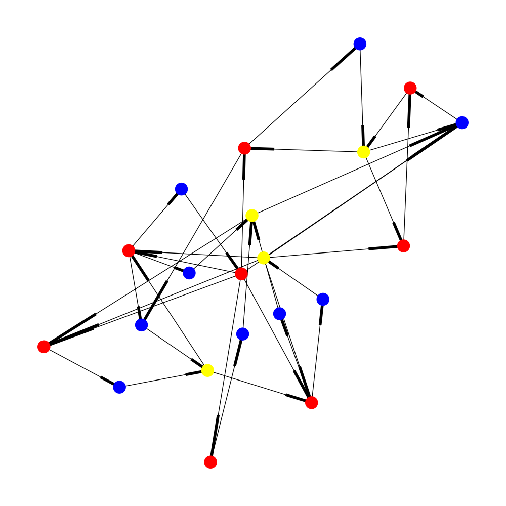
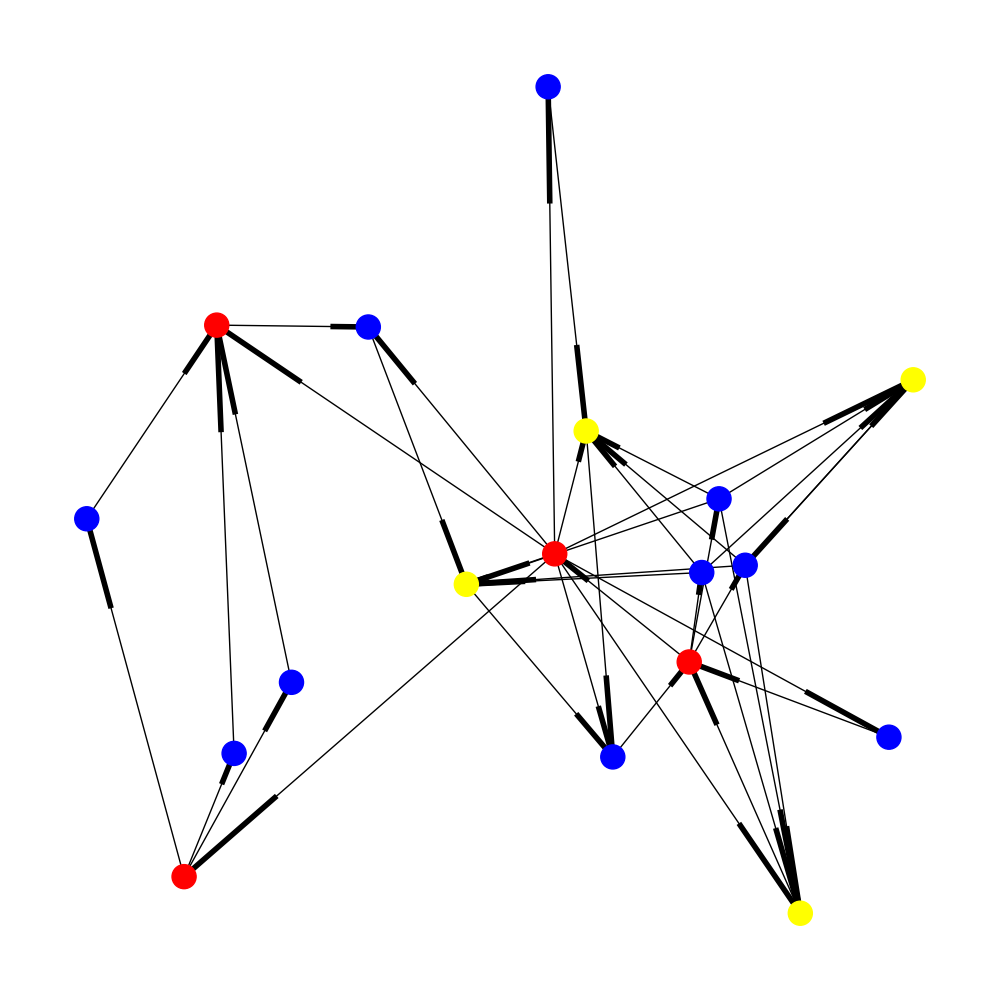
We identify the strongly connected components (SCC) in these networks with organized sets of taxpayers which can be related to anomalous financial activity. We show the largest SCC observed in 2015 and 2016 in Fig. 4. Remembering that links in the network correspond to transactions, the presence of these structures imply a circular flow of goods and services, which being related to nodes associated to EFOS, is possible that these sets of nodes carry out tax evasion practices such as the exchange of receipts of simulated transactions, which suggests that the unclassified RFCA in the SCC might be suspect of carrying out the same practices.

Monthly interaction networks

In this section we consider the interaction networks between taxpayers at the month timescale. Unlike the yearly interaction networks where we only took into account the emissions and receptions of the nodes associated with EFOS, in this case we consider the transactions between all three kinds of nodes (EFOS, alleged EFOS and unclassified RFCA). Nonetheless, as the whole set of transactions is huge, we need to define criteria to filter transactions to reduce the network into a manageable size.

Figure 5: Time behaviour of the logarithm of the subtotal of the transactions associated to emissions from EFOS (left panel) and alleged EFOS (right panel), the vertical dashed lines indicate the month of December of each year. Solid lines show the median and the dashed lines the interquartile range of the distribution. It can be seen that the transactions between EFOS, either definitive or alleged, correspond to amounts around tens of thousands and millions of pesos. We define this range of amounts as the EFOS activity regime, which we use to filter the links in the interaction networks.

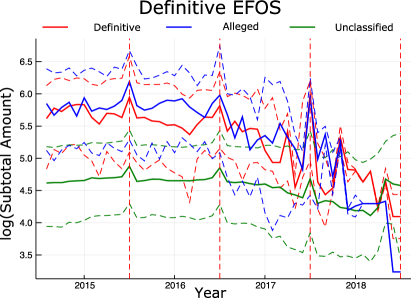
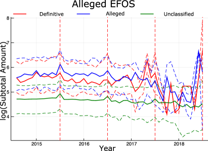
To this end, we obtain the distribution of the subtotal amounts before taxes of the transactions emitted by EFOS (for both definitive and suspect) to the remaining types of nodes. As can be seen in Fig. 5, the median of the distribution changes over time, showing an increase towards the end of the year. It is to be noted that the amounts of the transactions between EFOS are higher than those of the transactions between EFOS and unclassified RFCA, which suggests that EFOS make selective emissions whether the receiver of the transaction is an EFOS or arbitrary RFCA. We define the EFOS activity regime, as the amounts interval defined by the interquartile ranges of the amounts distribution obtained from the EFOS transactions. We only take into account links in the monthly interaction networks whose amount lies inside the EFOS activity regime. Once we have selected the relevant links in the monthly interaction networks between taxpayers, we obtain the largest SCC of the network, which e.g. for 2015 consists of 635,588 nodes.

We define the reach of the $i$-th node in the network at distance $d$, $r_{i}(d)$, as the fraction of nodes in the SCC up to a distance $d$ from the node, i.e.

$$\omega_{i}=\{j\;|\;d_{ij}\leq d\},$$ (1a)

$$r_{i}(d)=\frac{|\omega_{i}|}{N},$$ (1b)

where, $d_{ij}$ is the length of the shortest path length between nodes $i$ and $j$, $|\omega_{i}|$ is the number of elements in $\omega_{i}$, and $N$ is the number of nodes in the SCC.

If we now consider a set of nodes $\Omega$, we can calculate the mean reach of the set of nodes at distance $d$, $\langle R(d)\rangle_{\Omega}$, by

$$\langle R(d)\rangle_{\Omega}=\frac{1}{|\Omega|}\sum_{i\in\Omega}r_{i}(d),$$ (2)

where $\Omega$ represents either the set of nodes that correspond to EFOS or unclassified RFCA.

Figure 6: Mean reach, $R(d)$, as a function of distance $d$, for nodes that correspond to EFOS and to unclassified RFCA. $R(d)$ is higher for EFOS than for unclassified RFCA, which suggests that EFOS are more efficient to distribute their transactions in the network. Data correspond to January 2017 (left panel) and May 2017 (right panel).

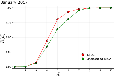
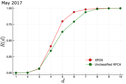
The topology of the network is such that, as can be seen in Fig. 6, the reach of EFOS is higher for distances $3<d<7$ than for the rest of the nodes. This suggests that EFOS are more efficient to distribute their transactions in the network, which can be related to mechanisms aimed to limit the traceability of their transactions. Following the reach behavior, we define the set of nearest neighbors of a node as the set of nodes at $d_{ij}<3$. We plot the distribution of close EFOS, for both a month and one year’s aggregates. From unclassified RFCA in Fig. 7, we see there are cases in which unclassified RFCA are close to more than 100 EFOS in one month.

Figure 7: Nearest EFOS to unclassified RFCA distribution for the monthly interaction networks (left panel) and one year’s aggregate (rigt panel). The number of close EFOS is a collusion indicator of unclassified RFCA in the EFOS operation networks. As can be seen in both panels, there are unclassified RFCA close to a large number of EFOS in both timescales.

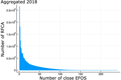
We use the number of close EFOS to unclassified RFCA in the interaction network as an indicator of their collusion in the EFOS operation networks, so that we can assume that an arbitrary RFCA close to a large number of EFOS, is more susceptible to take part in the same corrupt practices as EFOS, when compared to RFCA which are not as close to EFOS in the network.

We define for each one of the identified suspect RFCA, the EFOS proximity index, $\sigma_{i}(y)$, for the $i$-th node in the network for the year $y$, as que quotient of the total number of EFOS at $d_{ij}<3$ during the year, and the number of months these EFOS were close to the RFCA, i.e.

$$\sigma_{i}(y)=\frac{\mathrm{Close\;EFOS\;in\;}y}{\mathrm{Number\;of\;months\;they\;were\;close}}.$$ (3)

Note that the denominator can be less than 12, as there can be months in which the RFCA wasn’t close to any of the EFOS in the network. As the number of active EFOS in the network changes over time, we normalize the EFOS proximity index, which we express by $\hat{\sigma}_{i}$, with respect to the maximum observed during the year, i.e.

$$\hat{\sigma}_{i}(y)=\frac{\sigma_{i}(y)}{\max(\sigma_{i}(y))},$$ (4)

where $\hat{\sigma}_{i}(y)\in[0,1]$, this allows us to define a threshold to be used in all periods, $\theta_{\sigma}(y)$, which through the condition $\hat{\sigma}_{i}(y)\geq\theta_{\sigma}(y)$ with $\theta_{\sigma}(y)\approx 1$, allows us to select the more colluded suspect RFCAs for each year.

(a)

(b)

Figure 8: Normalized proximity index to EFOS distribution for suspect RFCA identified by the ANN and Random Forest models. This index is used as an extra validation criteria of the suspect list obtained from the Machine Learning models using characteristics observed in the interaction networks. We show the results for (a) 2015 and (b) 2016. Dashed lines represent the 25, 50 and 75% quartiles of the proximity index distribution.

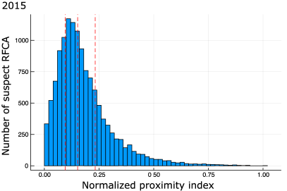
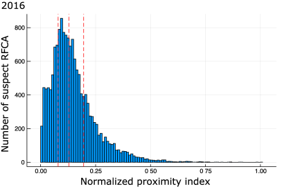
The description we’ve made of both yearly and monthly interaction networks between taxpayers, allowed us to identify features of the EFOS organization mechanisms and the local structure of the network around them, such as: their organization in small operation networks related to closed flows of CFDIs between them, and selective CFDI emissions between EFOS of much larger amounts than the transactions they make with unclassified RFCAs, which suggests that EFOS operate inside an activity regime defined by the amounts of their transactions (see Fig. 5). We have been able as well to quantify, by means of the reach of nodes in the network and the proximity index, the collusion of unclassified RFCAs inside the EFOS operation networks. These results suggest that complex networks analysis provides useful techniques with ample potential to describe and characterize corruption networks and operational mechanisms, which are yet to be fully explored.

3.4 Merging the classification methods

We obtain a list of suspect RFCAs from each Machine Learning classification method (ANN and Random Forest). It is to be noted that the training set for both of these methods, consisted of examples from the evaders already identified by the authorities, therefore, there is an inherent and implicit bias in our methods towards the mechanisms and assumptions used by the authorities to identify evaders. This bias in unavoidable due to the data we had available and it is important to take into account further methods to make a wider characterization of these and other evasion mechanisms.

We report the number of suspect RFCAs identified by each method in Table 6. The list obtained from the ANN corresponds to those RFCAs with an probability of belonging to the same class as EFOS $>0.8$. We use the same threshold for the probability assigned by the Random Forest model. The intersection of both suspect lists is contains 43,650 RFCA, which we consider to have a higher probability of being suspect evaders, as they were identified independently by two different methods.

Method	Classified as suspect	Unclassified
Artificial Neural Network	149,921	7,416,754
Random Forest	128,227	7,438,448

Table 6: Number of suspect RFCA identified by each classification method.

Suspect RFCA comparison with EFOS

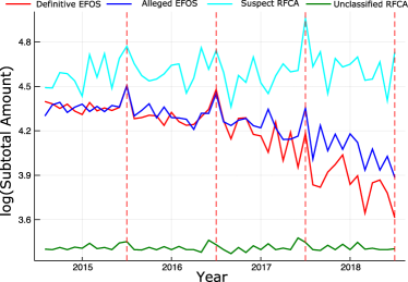
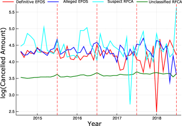
To compare the features of the suspect RFCAs identified by our classification methods with those of EFOS, we compute the distributions of the active and canceled amounts associated to their CFDI emissions. Active amounts correspond to the emitted and processed invoices, and canceled amounts correspond to those invoices that were canceled and not processed. The cancellation of CFDIs can be done freely and independently by taxpayers without an explicit authorization. As can be seen in Fig. 9, the distributions of these two variables are very similar for EFOS and the suspect RFCAs identified by our methods, while for unclassified RFCA, the distributions of these variables are different. Furthermore, in Fig. 10, we show the time behavior of the active and canceled amounts of the CFDIs emitted by the different RFCA groups (definitive EFOS, alleged EFOS and unclassified RFCAs). It can be seen that the difference between suspect and unclassified RFCAs is consistent for the whole analysis period, which sets these two groups (EFOS and suspect RFCA) apart from unclassified RFCA.

(a)

(b)

Figure 9: Boxplots for the distributions of the (a) logarithm of the total cancelled amount and (b) the active subtotal amount of the CFDI emitted by EFOS, suspect and unclassified RFCA. It can be seen that the distributions for EFOS and suspect RFCA are more similar between each other than when being compared with the distributions of unclassified RFCA.

(a)

(b)

Figure 10: Temporal behavior of the (a) Active subtotal amount and (b) Cancelled total amount for each one of the groups of RFCAs: definitive EFOS (blue), alleged EFOS (red), unclassified RFCAs (green) and suspect RFCAs (cyan). The vertical dashed lines correspond to December for each of the years studied. It can be seen that the EFOS and suspect RFCAs behavior differentiates from unclassified RFCAs.

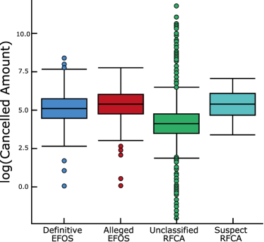
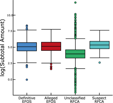
Number of close EFOS to suspect RFCA

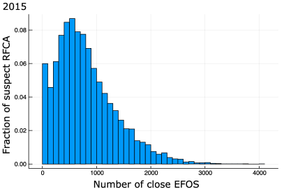
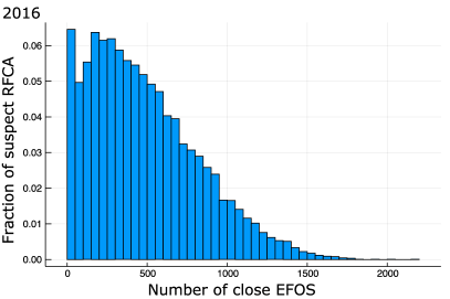
As it was discussed in Section 3.3, the EFOS reach in the interaction networks allows us to identify the number of close EFOS to unclassified RFCA in the network (where close means at a distance $d\leq 3$) and use it to select those RFCAs more immersed in the EFOS operation networks. Now, if we look at the suspect RFCAs identified by the classification methods, and compute the number of close EFOS in a whole year, we observe that they are close to a large number of EFOS (see Fig. 11), which suggests that the suspect RFCAs in the intersection of the lists obtained from both classification method are colluded with the EFOS identified by the authorities and gives us confidence about our methods. It is to be noted that the closeness to EFOS wasn’t part of the set of features used by the classification methods (ANN and Random Forest) to identify suspect RFCAs, as they were based only on CFDI data.

(a)

(b)

Figure 11: Total of close EFOS the suspect RFCAs identified by our classification methods for (a) 2015 and (b) 2016. It can be seen that a suspect RFCA are close to a large number of EFOS, which indicates that these RFCAs are immersed into the EFOS operation networks.

As we show in Table 7, 81.52% of the suspect RFCA are legal persons, which suggests that most part of the emitted CFDI linked with allegedly simulated operations is made between companies or businesses. This can be due to the fact that, in this case the legal responsibility of possible illicit operations, falls to a legal entity and not a natural person. In table 7, we also show that 91.15% of the suspect RFCA were active at the moment of the elaboration of the study, and less than 1% of them had a cancelled or suspended status, which shows that most of the suspect RFCA are economically active, and thus susceptible of being investigated.

Taxpayer type	Percentage of suspect RFCAs
Legal	81.52%
Natural	10.22%
Without info	8.3%

Status	Percentage of suspect RFCAs
Active	91.15%
Cancelled	0.13%
Suspended	0.46%
Without info	8.3%

Table 7: Type of taxpayer and status of the suspect RFCA identified by the classification methods. Most of them were active legal taxpayers at the moment, which made them susceptible of being investigated by the authorities.

Using the data contained in the CFDI, we define the potential tax collection associated to an arbitrary RFCA, $\mathrm{rec_{VAT}}\phi_{i}$, as the difference between the total nominal tax obtained by the income CFDI emitted during the year, $\mathrm{VAT_{Nom}}_{i}$, and the payed tax reported in their tax statements, $\mathrm{VAT_{Payed}}_{i}$, i.e.

$$\mathrm{rec_{VAT}}\phi_{i}=\sum\mathrm{VAT_{Nom}}_{i}-\mathrm{VAT_{Payed}}_{i},$$ (5)

so that, we define the total nominal tax collection that correspond to the set of suspect RFCA, $\mathrm{REC_{IVA}}\phi$ as:

$$\mathrm{REC_{VAT}}\phi=\sum_{i}\mathrm{rec_{VAT}}\phi_{i}.$$ (6)

We use the income CFDI emitted by the identified suspect RFCA between the years 2015 and 2018, and their yearly tax statements, which include the total VAT payed by them. We believe that the information of the emitted CFDI allows us to have a better description of the economical activity and evasion mechanisms, because the income amounts declared in the tax statements is vulnerable of manipulation, and may not reflect reality, mostly because we are dealing with taxpayers suspects of simulating operations. A significative difference between income amounts from CFDI emissions and tax statements could be a indicator of possible illicit practices.

3.5 Yearly evasion estimates

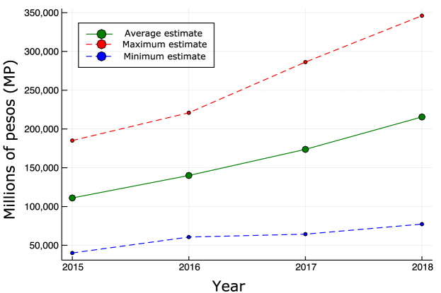
As we discussed in section 3.3, the number of close EFOS to a RFCA in the interaction networks, is an indicator of their collusion level in the sub-networks associated with EFOS, so that we can assume that a suspect RFCA close to a larger number of definitive and alleged EFOS, is much more susceptible to conduct the same practices as EFOS. With this in mind, we calculate evasion estimates for each year between 2015 and 2018, based on the suspect RFCA closest to EFOS in the monthly interaction networks for each year, which correspond between 28% and 38% of all suspect RFCA.

VAT evation estimates (MP)
Year	Minimum	Average	Maximum
2015	40,097.27	111,048.36	185,087.23
2016	60,626.86	140,041.13	220,922.03
2017	64,377.11	173,717.06	286,273.35
2018	77,318.59	215,518.71	346,106.32
Year average	60,604.96	135,081.31	259,597.23

Unique suspect RFCA
Year	Minimum estimate	Maximum estimate
2015	2,686	10,767
2016	3,132	12,510
2017	3,461	13,743
2018	3,541	14,080
Total	7,677	17,769

Figure 12: Maximum and minimum VAT evasion estimates in millions of pesos (MP) associated to the emission of CFDI of potentially simulated operations from suspect RFCA in the period 2015 -2018. We present as well the number of unique RFCA used for the calculations for each year. We estimate the number of unique suspect RFCA to be between 7,677 and 17,769.

The EFOS proximity index threshold, $\theta_{\sigma}$, allows us to define minimum and maximum values for VAT evasion estimates. The maximum estimated value corresponds to all identified suspect RFCA, and minimum values to estimates based on suspect RFCA of the last quartile (top 25%) of the EFOS proximity index distribution, which correspond to 7,677 unique suspect RFCA with CFDI emissions between 2015 and 2018, which corresponds to an average estimate of 60,604.96 millions of pesos per year. The VAT evasion estimates in Fig. 12 should not be considered as final values, as there might exist VAT evasion mechanisms different from the simulation of operations, which we don’t take into account in this work. Furthermore, it is important to mention that there is an additional uncertainty because, it is not possible to determine precisely the fraction of simulated and real transactions made by the suspect EFOS with the available information. Because of this situation, we assume the 100% of the emitted CFDI by suspect RFCA as simulated operations. A follow up study focused in the traceability of the emitted CFDI could help determine the fraction of simulated operations, which would allow us to make a more precise VAT evasion estimate.

4 Discussion

We have shown that it is possible to use tools from network science and machine learning to automatically identify patterns of tax evaders similar to those that humans already identified. This is promising, but should also be taken with caution. It is promising, because similar techniques could be applied in a broad variety of areas: money laundering, bribery practices, and other illegal activities. In principle, this would benefit society. However, one should also be aware of the limits of these methods. First, the patterns identified are based on those already known to humans. This means that different patterns of tax evasion will not be identified. Second, using these techniques to curb illegal activities would promote criminals to use alternative patterns that are not identified, so an arms race would ensue. The tools have a relevant potential, but by themselves, are not a final solution. Finally, there is always the probability of misidentifying honest citizens or companies for wrongdoers, simply because they have similar statistical patterns. Thus, these methods can be used to identify and prioritize potential suspects from a huge pool, but the final decision has to be made by humans.

In general, our work illustrates the potential of recent technology to solve different problems exploiting large data sets, computing power, and sophisticated statistical techniques. Still, the limits of this technology are yet to be defined properly, which has led to much hype and overconfidence. Also, ethical issues must be considered for the use of this technology. As more applications are developed, we can learn from them to better situate the benefits and risks of using network science, machine learning, and related techniques to address social problems.