Beyond Simple AGN Unification with Chandra-observed 3CRR Sources at $0.5<z<1$

Abstract

Low-frequency radio selection finds radio-bright galaxies regardless of the amount of obscuration by gas and dust. We report Chandra observations of a complete 178 MHz-selected, and so orientation unbiased, sample of 44 $0.5<z<1$ 3CRR sources. The sample is comprised of quasars and narrow-line radio galaxies (NLRGs) with similar radio luminosities, and the radio structure serves as both an age and an orientation indicator. Consistent with Unification, intrinsic obscuration (measured by $N_{\rm H}$, X-ray hardness ratio, and X-ray luminosity) generally increases with inclination. However, the sample includes a population not seen in high-$z$ 3CRR sources: NLRGs viewed at intermediate inclination angles with $N_{\rm H}$ $<10^{22}$ cm^-2. Multiwavelength analysis suggests these objects have lower $L/L_{\rm Edd}$ than typical NLRGs at similar orientation. Thus both orientation and $L/L_{\rm Edd}$ are important, and a “radiation-regulated Unification” provides a better explanation of the sample’s observed properties. In comparison with the 3CRR sample at $1<z<2$, our lower-redshift sample shows a higher fraction of Compton-thin NLRGs (45% vs. 29%) but similar Compton-thick fraction (20%), implying a larger covering factor of Compton-thin material at intermediate viewing angles and so a more “puffed-up” torus atmosphere. We posit that this is due to a range of $L/L_{\rm Edd}$ extending to lower values in this sample. In contrast, at high redshifts the narrower range and high $L/L_{\rm Edd}$ values allowed orientation (and so simple Unification) to dominate the sample’s observed properties.

1 Introduction

Active Galactic Nuclei (AGN) are among the most luminous non-transient objects in the Universe and are responsible for the majority of accretion (as opposed to stellar) power output. Their activity is centered in a small nuclear region (the central engine), where the standard model invokes a supermassive black hole surrounded by accreting gas forming an accretion disk (emitting in the visible–UV–soft-X-rays) and a hot corona (emitting hard-X-rays). Much of this radiation is then absorbed and reprocessed by gas and dust (emitting in the infrared) in a disk/torus-like structure surrounding the accretion disk, as described by the Standard Unification model (Barthel, 1989; Antonucci, 1993; Urry & Padovani, 1995; Netzer, 2015). In the Standard model, observationally different AGN and radio galaxies are related to each other via the viewing angle. The broad-line (“Type 1”) AGN (Seyfert 1s, quasars, broad-line radio galaxies) are viewed along the poles of the dusty disk/torus, where the (“face-on”) view of the central engine and the broad emission line region (BLR) is unobscured. The narrow-line (“Type 2”) AGN (Seyfert 2s, narrow-line radio galaxies) are viewed edge-on to the torus, so the central engine and the BLR are blocked from view, and only the narrow emission lines, formed farther out, are visible. In some Type 2s, the emission from the central engine reveals itself in scattered polarized light (Zakamska et al., 2005).

In its most basic version (Antonucci, 1993), Unification assumes a compact, smooth torus (Pier & Krolik, 1992; Granato et al., 1997) with the same opening angle for all AGN independent of their intrinsic luminosity. Simple Unification is an oversimplification (already pointed out by Antonucci in his 1993 review), and a “receding torus model” where the inner sublimation radius increases with AGN luminosity, was introduced (Falcke et al., 1995; Lawrence, 1991) to explain the observed decrease of the fraction of Type 2 AGN with increasing luminosity. Further refinement of Unification and the introduction of clumpy torus models (Nenkova et al., 2008a, b; Hönig et al., 2010; Stalevski et al., 2012; Siebenmorgen et al., 2015) introduced the covering factor as an additional, independent variable (Elitzur, 2012; “realistic” Unification). In this scenario, AGN at a given intrinsic luminosity have a distribution of covering factors. The ratio of Type 2 to Type 1 AGN depends on the mean covering factor of the sample, and the Type 2s will preferentially be drawn from a population of AGN that have covering factors higher than the mean, while the Type 1s are drawn from a population with covering factors below the mean. It was recently shown (Ricci et al., 2017; Ezhikode et al., 2017) that the covering factor of the obscuring dusty gas is strongly dependent on a fundamental parameter of the central engine – the Eddington ratio $L/L_{\rm Edd}$ – and is lowest in AGN with the highest $L/L_{\rm Edd}$. This dependence is explained as due to clearing out of the (Compton-thin) gas and dust clouds within the opening angle of the torus via radiation pressure, creating larger torus opening angles in sources with higher $L/L_{\rm Edd}$. Labelled “radiation-regulated Unification”, the effect results in the probability of finding an obscured AGN increasing with decreasing $L/L_{\rm Edd}$ ratio.

Obscuration in AGN is not only highly anisotropic and likely $L/L_{\rm Edd}$ dependent, it is also strongly wavelength-dependent, which will cause complex selection effects and result in strong biases against specific subsets of AGN depending on the wavelength of a sample’s selection. A significant fraction of the AGN population is largely unobserved as was demonstrated by the Cosmic X-ray Background (CXRB, Gilli et al., 2007), which requires equal numbers of unobscured and moderately (Compton-thin) obscured ($10^{21}<$ $N_{\rm H}$/cm^-2 $<10^{23}$) sources, and a comparable number of highly-obscured, Compton-thick ($N_{\rm H}$ $\geq 1.5\times 10^{24}$ cm^-2) AGN. This last, Compton-thick population has not yet been found. The Two Micron All-Sky Survey (2MASS) revealed a significant population of red, moderately obscured ($10^{21}<$ $N_{\rm H}$/cm^-2 $<10^{23}$, Wilkes et al., 2002, 2005; Kuraszkiewicz et al., 2009a, b) Type 1 and Type 2 AGN with a number density comparable to that of blue optically-selected (Type 1) AGN at low redshifts (Cutri et al., 2002). The Sloan Digital Sky Survey (SDSS), using optical color selection techniques (Richards et al., 2003), and the Hamburg Quasar Spectral Survey (Hagen et al., 1995) revealed many Type 1 AGN with much redder colors than those found in AGN samples typically selected based on blue optical colors. Chandra and Spitzer facilitated many deeper, multi-wavelength surveys such as GOODS (Giavalisco et al., 2004), SWIRE (Lonsdale et al., 2003), Boötes (Hickox et al., 2007), ChaMP (Kim et al., 2007), COSMOS (Scoville et al., 2007), AEGIS (Davis et al., 2007; Eisenhardt et al., 2004), CANDELS (Grogin et al., 2011), and HERMES (Oliver et al., 2012) which through hard-X-ray and/or infrared (IR) selection probed deeply into the AGN population revealing larger numbers of obscured AGN than the traditional optical surveys (Alexander et al., 2003; Polletta et al., 2006). However, even as more are being found, bias against finding Compton-thick AGN remains. They are difficult to find as their direct light is obscured even at Chandra and XMM-Newton energies ($<$10 keV). Harder X-ray surveys carried out using Swift/BAT, NuSTAR and INTEGRAL, (Burlon et al., 2011; Aird et al., 2015; Sazonov et al., 2012) also miss the most Compton-thick AGN, which is not surprising as direct X-ray light from NGC 1068, a canonical nearby Type 2, is undetected to energies $\gtrsim$100 keV (Matt et al., 1997). Selection at IR wavelengths (Lacy et al., 2004; Stern et al., 2005) provides a way to search for highly obscured AGN, but these are difficult to identify among a much larger population of IR galaxies (Barmby et al., 2006; Park et al., 2010).

Low-frequency radio selection (although limited to bright radio-loud sources) is based on the optically thin and nearly isotropic emission from the extended radio lobes. It is largely independent of orientation and provides a reliable way to assemble radio-loud AGN samples that are complete and free of orientation-related bias. Accordingly, the 3CRR catalog of Laing et al. (1983) delivers a complete, randomly oriented sample out to redshift $z=2.5$ down to a limiting flux density of 10 Jy at 178 MHz and includes 173 radio galaxies and quasi-stellar radio sources (quasars). At these low frequencies 3CRR sources are dominated by emission from the extended radio lobes resulting in a sample free of orientation bias.

In the present work, we focus on the complete (orientation unbiased) subset of $0.5<z<1$ 3CRR sources and analyze X-ray, IR, optical, and radio properties in relation to orientation and obscuration effects, thus constraining the properties and geometry of the obscuring material. This paper extends our studies of the $1<z<2$ 3CRR sample (Wilkes et al., 2013), allowing investigations of redshift and luminosity-dependent effects on obscuration relative to orientation and testing Unification schemes. The medium-$z$ 3CRR sample is described in Section 2. The supporting, non-X-ray, data are presented in Section 3. The analysis of new and existing Chandra X-ray data is given in Section 4, and the relation of the X-ray, radio, and infrared properties to obscuration and orientation in Section 5. The discussion of the results in the context of Unification models is presented in Sections 6 and 7, and a summary is given in Section 8. Throughout the paper we assume a $\Lambda$CDM cosmology with $H_{0}=69.6$ km s^-1 Mpc^-1, $\Omega_{M}=0.286$, and $\Omega_{\Lambda}=0.714$ (Bennett et al., 2014)

2 The Sample

The 3CRR catalog (Laing et al., 1983) contains a complete, 178 MHz radio-flux limited sample of 173 quasars and radio galaxies brighter than 10 Jy extending to $z=2.5$. At these low frequencies, the emission, whether for radio galaxies or quasars, is dominated by extended radio lobes, which are optically thin and emit nearly isotropically, resulting in a sample that is unbiased by the effects of orientation and obscuration. The radio morphologies, radio sizes, and lobe separations are well known for all 3CRR sources. The higher-frequency 5 GHz radio data (where the radio core emission is more pronounced than in low frequency radio) provide an independent estimate of orientation via the radio core fraction (Orr & Browne, 1982) $R_{\rm CD}$ $\equiv F_{\rm core}$(5 GHz)$/F_{\rm lobe}$(5 GHz), which is defined as the ratio of the beamed radio core (unresolved on arcsecond scales) to the extended, nearly isotropic emission from the radio lobes. Additionally the lengths of the radio jets provide an estimate of the AGN ages (e.g. Podigachoski et al., 2015).

Wilkes et al. (2013) studied the $1<z<2$ subset of the 3CRR sources (hereafter the high-$z$ sample). In this work we focus on the $0.5<z<1$ 3CRR sample (hereafter the medium-$z$ sample; Table 1), which includes 44 sources. All 3CRR sources at $z>0.5$ are of Fanaroff-Riley type II (FR II; Fanaroff & Riley, 1974) characterized by powerful double radio lobes (often extending far beyond the host galaxy) that are edge-brightened (i.e., having bright hotspots at the ends of their lobes) and showing high radio powers $P_{\rm 178\,MHz}>10^{26.5}$ W Hz^-1 sr^-1. At these redshifts, the radio luminosities are comparable to those of the most powerful radio sources found at earlier epochs ($2.5<z<6$) when the quasar activity peaked. This ensures that the objects in our sample are powerful AGN. Studies of redshift and size distributions (Singal, 1993) and the detection of X-ray emission (Section 4) confirm the presence of an AGN in all sources. All 3CRR sources in the medium-$z$ sample have now been observed with Chandra.

The medium-$z$ sample can be divided into two types:

1. broad-line radio galaxies and quasars, hereafter collectively referred to as quasars (14 objects),

2. narrow-line radio galaxies (NLRGs; 29 sources) and 1 low-excitation radio galaxy (LERG), hereafter collectively referred to as radio galaxies.

Most of the 3CRR quasars and radio galaxies have steep radio spectra ($\alpha>0.5$; $F_{\nu}\propto\nu^{-\alpha}$) and extended, lobe-dominated radio emission at 178 MHz. However, six quasars and three NLRGs with steep radio spectra have compact ($<$10 kpc) structure. These are compact steep spectrum (CSS) sources (O’Dea, 1998; Fanti et al., 1985; An & Baan, 2012), thought to be either evolutionarily young or to have their jets frustrated due to interaction with large amounts of material. There are no strongly beamed, radio core-dominated quasars in this sample, with only two marginally core-dominated radio sources (3C 380 with log $R_{\rm CD}$ $=0.18$ and 3C 216 with log $R_{\rm CD}$ $=0.15$ ), so beamed emission is not dominant across the sample.

The one LERG (Hine & Longair 1979) in the sample is 3C 427.1. LERGs have inherently weak (unobscured) X-ray (Hardcastle et al., 2009) and mid-IR emission (Ogle et al., 2006) and are possibly powered by a radiatively inefficient accretion flow (Hardcastle et al., 2009; Evans et al., 2006; Ogle et al., 2006; Ghisellini & Celotti, 2001). They reside mostly in FRI-type radio sources (Fanaroff & Riley, 1974) or lower-radio power ($P_{\rm 178\,MHz}$ $\sim$ 10^26.5 W Hz^-1 sr^-1) FRII-type sources (Chiaberge et al., 2002; Grimes et al., 2004). 3C 427.1 is one of the latter.

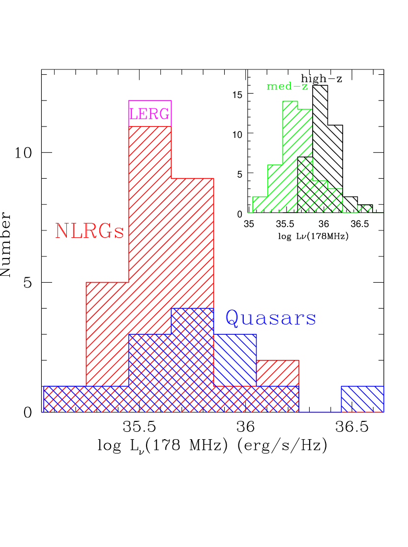
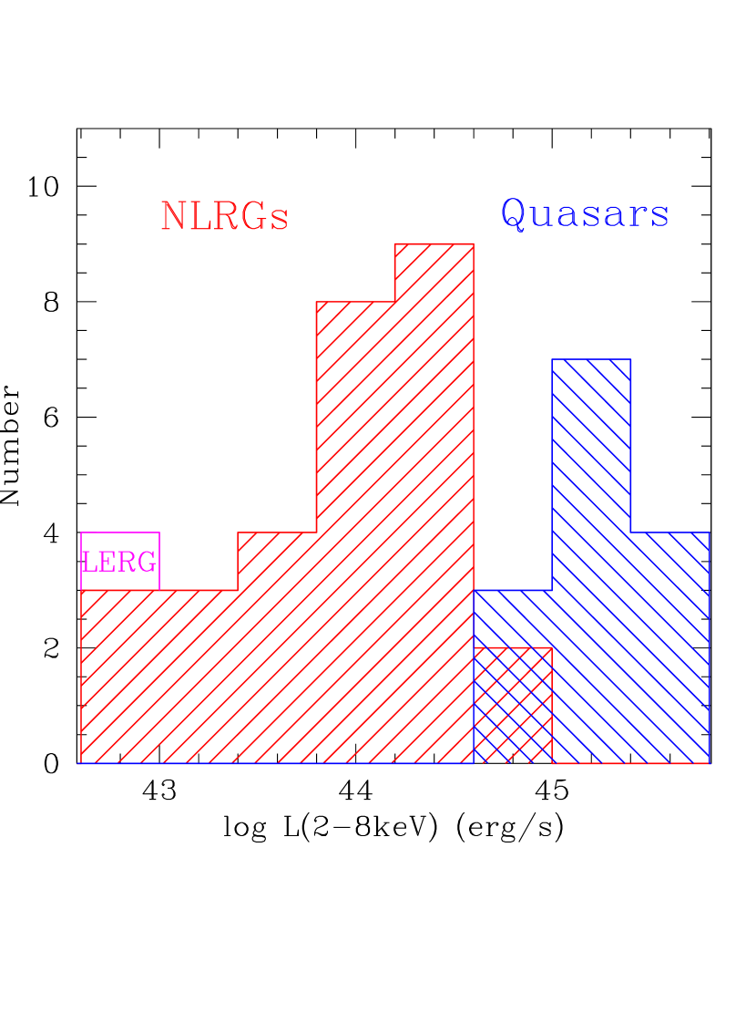
Figure 1: Left: The distribution of the total, rest-frame, 178 MHz radio luminosity density $L_{\nu}(178\,{\rm MHz})$ for the medium-$z$ ($0.5<z<1$) 3CRR sample. The blue histogram shows quasars, the red histogram NLRGs, and the LERG is plotted in magenta. The inset in the upper right corner, shows the distribution of $L_{\nu}(178\,{\rm MHz})$ for all sources in the medium-$z$ 3CRR sample in green and the high-$z$ 3CRR sample (Wilkes et al., 2013) in black. Right: The distribution of the 2–8 keV hard-X-ray luminosity uncorrected for intrinsic absorption for the medium-$z$ sample. Quasars are plotted in blue, NLRGs in red, and the LERG in magenta. The range of radio luminosities is narrow ($\sim$1.5 dex) with quasars and NLRGs having similar 178 MHz luminosities (a proxy for intrinsic AGN luminosity). The hard-X-ray luminosity distribution covers a wider range ($\sim$3 dex) with the NLRGs being 10-1000 times fainter in X-rays than quasars, which can be explained by higher intrinsic obscuration in NLRGs (Section 5.1).

The medium-$z$ 3CRR quasars and NLRGs occupy the same $\sim$1.5 dex range in 178 MHz radio luminosity density(Figure 1 left), where $10^{35.2}<L_{\nu}(178~{}{\rm MHz})$/erg s^-1 Hz${}^{-1}<10^{36.6}$. The K-S test reveals no difference in $L_{\nu}(178~{}{\rm MHz})$ distributions of quasars and NLRGs. In comparison, the distribution of radio luminosities in the high-$z$ 3CRR sample (Wilkes et al., 2013) is narrower (1 dex) and covers higher radio luminosities $10^{35.9}<L_{\nu}(178~{}{\rm MHz})$/erg s^-1 Hz${}^{-1}<10^{36.8}$ (Figure 1 left: inset).

Because of their high flux densities ($F_{\nu}(178\,{\rm MHz})>$ 10 Jy), their high luminosities, the complete nature of the survey, and the availability of comprehensive multi-wavelength data, the 3CRR sources constitute an excellent AGN sample with which to study orientation-based effects and test Unification schemes. One caveat is that only 10% of the AGN population is radio loud, and caution is required when generalizing results to the whole AGN population. Additionally, the radio-emitting plasma may affect the opening angle of the torus (Falcke et al., 1995) and contribute to the X-ray emission (especially in strongly beamed sources).

3 Supporting data

3.1 Radio Data

The 5 GHz radio core and extended radio lobe flux densities have been compiled from the literature. The radio core, the total (core+lobe) flux densities, and the total luminosity densities at 5 GHz ($L_{\nu}(5\,{\rm GHz})$) are presented in Table 1. The radio core fraction $R_{\rm CD}$ is also given, which is often used as an orientation indicator in radio-loud AGN (Orr & Browne, 1982; Ghisellini et al., 1993) and gives, in general, an estimate of the inclination angle accurate to within $\pm$20° (Wills & Brotherton, 1995) and in the case of the $z\geq 1$ 3CRR sources to $\pm$10° or less (Marin & Antonucci, 2016). When available, we used the same reference for the radio core and extended radio lobe luminosities when calculating $R_{\rm CD}$. Other references were checked for flux consistency. For sources with no 5 GHz data, the 8 GHz flux density was used to estimate the 5 GHz flux density, assuming a radio spectral index of $\alpha=0.7$ (typical of extended emission from radio galaxies e.g., Dennett-Thorpe et al., 1999) for the radio lobes and $\alpha=0.3$ (a compromise between a flat spectrum and steep spectrum core) for the radio core (where $F_{\nu}\propto\nu^{-\alpha}$). In the medium-$z$ 3CRR sample, log $R_{\rm CD}$  spans values from 0.15 to less than $-$3.5, which according to Marin & Antonucci (2016) correspond to a range of viewing angles measured in respect to the radio jets that range between 8° (close to pole-on) and 90° (perpendicular to the jet or edge-on to the torus).

3.2 IR Data

Spitzer (Werner et al., 2004) IRAC and MIPS photometry has been obtained and analyzed for the full 3CRR sample (Haas et al., 2008 for $z>1$ and Ogle et al., 2006 for $z<1$ sources). IRS spectroscopy is also available for sources in the redshift range $0.4<z<1.4$ (Cleary et al., 2007 for $0.4<z<1.2$ and Leipski et al., 2010 for $1<z<1.4$). All sources were observed in the far-IR during Herschel guaranteed time (PI Barthel) with PACS and SPIRE, and their IR SEDs (including 2MASS, WISE, Spitzer, and Herschel data) were analyzed by Podigachoski et al. (2015) for $z>1$ and Westhues et al. (2016) for $z<1$. The near-to-mid-IR (3–40$\mu$m) emission, dominated by the AGN, was found to be stronger in quasars than in radio galaxies, while the far-IR component, dominated by dust heated by star formation, is comparable in strength for the two classes. The difference in the mid-IR emission is consistent with the Unification scenario where the hot dust from the inner regions is directly visible in face-on quasars but obscured in NLRGs, which are viewed edge-on to the dusty torus. At $z<1$, an additional population of weak mid-IR AGN was found (LERGs and weak-MIR sources), possibly representing a different class of objects (nonthermal, jet-dominated with low accretion power) or different evolutionary stage from the mid-IR-bright sources (Ogle et al., 2006) .

4 X-ray Data

Of the 44 sources in the present sample, fourteen (7 quasars 3C 207, 254, 263, 275.1, 309.1, 334, 380 and 7 NLRGs 3C 6.1, 184, 228, 280, 289, 330, 427.1) had archival Chandra observations. One of these (3C 184) was also observed with XMM. For the remaining 30 sources Chandra ACIS-S observations of 23 sources were obtained (PI Kuraszkiewicz, proposal number 14700660) between 2013 Jan 21 and Oct 20 followed by observations of 7 sources (PI Massaro proposal number 15700111; between 2014 Jun 15 and 2015 May 20 (Massaro et al., 2018). The exposure times were set to ensure detection at flux levels expected for NLRGs and quasars as a function of redshift. Sub-arrays were used for the brightest quasars to avoid pileup. The nuclei of all but two sources (3C 220.3, 441) were detected. There is a wide range of signal-to-noise ($S/N$) ratios extending from a few net counts for the faintest NLRGs to $\sim$10000 net counts for the brightest quasars found in the archive (3C 207, 334). All Chandra observations are listed in Table 1 together with references to the existing Chandra and XMM data and spectral analysis.

The X-ray emission from radio-quiet AGN includes multiple components (Mushotzky et al., 1993): 1) an accretion-related power-law dominating the X-ray emission of luminous broad-lined AGN, absorbed in narrow-lined AGN, 2) a soft-X-ray excess, linked to the accretion disk, 3) reflected emission from hot and/or cold material surrounding the nucleus, 4) emission lines (Ogle et al., 2003), and 5) scattered nuclear light. Components 3, 4, and 5 become more significant in AGN with higher inclination angles, where the direct nuclear light is obscured (Mushotzky et al., 1993).

The X-ray emission of radio-loud AGN additionally includes non-thermal, synchrotron and/or inverse-Compton components associated with radio structures: jets, lobes, and hot spots (resolved with the high spatial resolution of Chandra  Wilkes et al., 2012; Worrall, 2009; Harris & Krawczynski, 2006) and jets dominating the emission of beamed, core-dominated (face-on), broad-lined, radio-loud AGN, which have on average $\sim 3\times$ higher soft X-ray luminosity and harder spectra in comparison with the radio-quiet AGN (Zamorani et al., 1981; Wilkes & Elvis, 1987; Worrall et al., 1987; Worrall & Wilkes, 1990; Miller et al., 2011, but see Zhu et al., 2020 who suggest a corona-jet interpretation). The amount of X-ray excess jet emission, above that expected from radio-quiet AGN, depends on the radio spectral slope and radio loudness and is a factor 0.7–2.8$\times$ higher for radio-intermediate quasars, $\sim$3$\times$ higher for radio-loud quasars and 3.4–10.7$\times$ higher for extremely radio-loud (strongly beamed sources). The X-ray jet-linked emission is less beamed (has a lower bulk Lorentz factor) than the radio jet emission (Miller et al., 2011). At $z<1$, it is possible to distinguish or place limits on the relative contributions from nuclear jet- and accretion-related X-ray components (Hardcastle et al., 2009; Evans et al., 2006; Belsole et al., 2006) in the higher signal-to-noise X-ray data. However, none of the sources in our sample are strongly beamed in our line of sight, and therefore the X-ray jet component is not expected to be strong (Hardcastle & Worrall, 1999).

4.1 Data Processing and Analysis

The Chandra data, both new and archival, were reprocessed using the standard pipeline to apply the latest calibration products appropriate for their observation dates and assure that processing was uniform across the sample. The counts for each source were extracted from a 2$\farcs$2 radius circle (to enclose the full point-spread function) centered on the radio core coordinates or when not available on the AGN X-ray position (Table 1). The background counts were extracted from an annulus with inner and outer radii of 15″ and 35″, respectively centered on the AGN, then scaled for area and subtracted to determine the net counts for each source. In a few sources, the background annulus was adjusted to exclude bright incidental X-ray sources. For nine sources (3C 172, 175, 228, 263, 265, 268.1, 330, 334, 340, 337, 441) for which the radio lobes showed substantial and extended X-ray emission, two circular regions with a 15″ radius lying outside the extended emission were used for background count estimation.

We use the following X-ray energy bands: broad ($B=0.5-8.0$ keV), soft ($S=0.5-2.0$ keV), and hard ($H=2.0-8.0$ keV). The broadband net source and background counts for each source are given in Table 2 (columns 3 and 4). The soft and hard band source and background counts were used to calculate hardness ratios (column 14).

4.2 Initial Flux Estimate from Srcflux: low count sources

To provide uniformly derived X-ray fluxes, the X-ray data for Chandra-observed sources were initially processed with Srcflux, a program in CIAO (Chandra Interactive Analysis of Observations; Fruscione et al. 2006), which is particularly useful in calculating the net count rates and fluxes in low count sources, where spectral fits are poorly constrained. Srcflux performs no spectral fits but instead fits the normalization based on the observed count rate for an assumed source spectrum and source and background regions. This results in fluxes estimated in a consistent manner, particularly for sources with highly absorbed or complex spectra and low $S/N$ data. We assumed a power-law spectrum with a canonical photon index $\Gamma=1.9$ (Just et al., 2007; Mushotzky et al., 1993) and Galactic absorption characterized by the equivalent hydrogen column density from Dickey & Lockman (1990) and quoted in Table 1. The same source and background regions as described in Section 4.1 were used. The “srcflux fluxes” and “srcflux luminosities” (K-corrected assuming a power-law with $\Gamma$=1.9) in the 0.5–8 keV range are given in Table 2 (columns 5 and 6). We will use these values as X-ray fluxes and luminosities throughout the paper for sources with $<$10 counts.

4.3 Spectral Fits

We performed X-ray spectral modeling of all sources in the sample with Sherpa (Freeman et al., 2001), a modeling and fitting package in CIAO. We used the Levenberg-–Marquardt optimization method with the $\chi^{2}$ statistic including the Gehrels variance function, which allows for a Poisson distribution for low-count sources. First a power-law with a canonical photon index $\Gamma=1.9$ and Galactic absorption was fit to binned spectra. For sources with $\geq$30 net counts, a second step including intrinsic absorption ($N_{\rm H}$) at the redshift of the source was added to the fit. For sources with $\gtrsim$700 net counts (mostly quasars), the power-law photon index was then freed in the final spectral fit. The results of the analysis are presented in Table 2. Significantly detected $N_{\rm H}$, indicating absorption in excess of the Galactic column density, is most likely absorption intrinsic to the quasar associated with the nucleus and/or the host galaxy. Although unlikely, a contribution from absorption by intervening material/sources along the line-of-sight cannot be ruled out.

For eight archival sources with more than a few thousand counts resulting in $\delta>$5% pileup, the CIAO pileup model (jdpileup) was included in the spectral fits. The pileup fraction is reported in Table 3, and the pileup corrected fluxes are presented in Table 2.

4.4 Complex Spectra

Several NLRGs displayed complex X-ray spectra. In particular 3C 265, 280, 330 showed excess soft X-ray emission above the absorbed primary power-law. This soft excess may be due to thermal emission from a surrounding cluster, emission from the accretion disk or inner region of the jets, intrinsic AGN emission visible due to partial covering of the AGN, or scattered emission from material close to the nucleus. For example 3C 265, a NLRG, shows a Sy1 spectrum in visible, polarized light (Véron-Cetty & Véron, 2006), implying scattered intrinsic AGN emission which may extend to the X-rays. Four galaxies, 3C 184, 265, 330, 427.1 show a strong 6.4 keV fluorescent Fe K$\alpha$ line arising from the reflection of the hard X-ray power-law on the (relatively) cold matter in an accretion disk or torus (Fabian et al. 2000 and references therein). Higher $S/N$ XMM-Newton data of 3C 184 require a soft excess and $N_{\rm H}$ $=4.9^{+2.2}_{-1.2}\times 10^{23}$ cm^-2 (Belsole et al., 2006). 3C 265 and 3C 330 display both a soft excess and a Fe K$\alpha$ line. The soft excess and the Fe K$\alpha$ line become pronounced in the heavily obscured sources, when the contribution of the intrinsic power-law is significantly reduced.

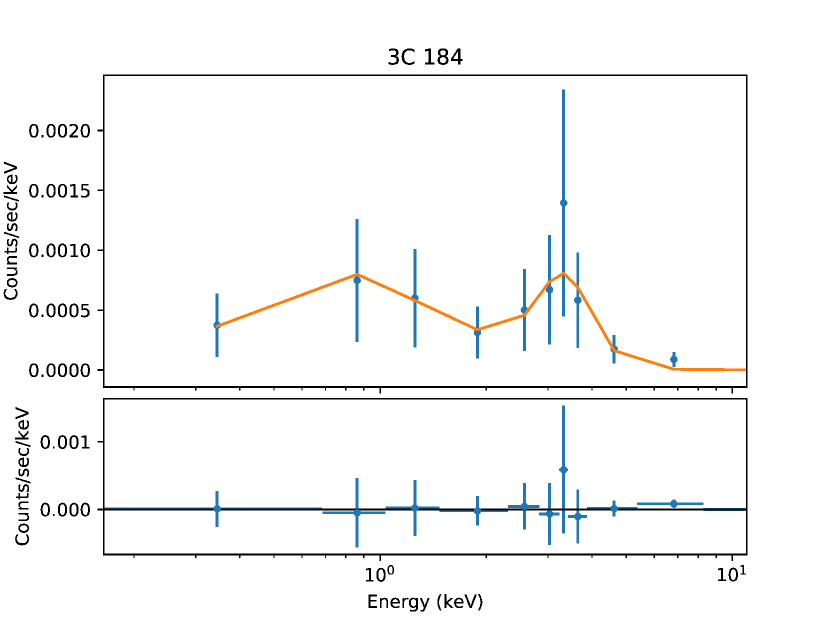
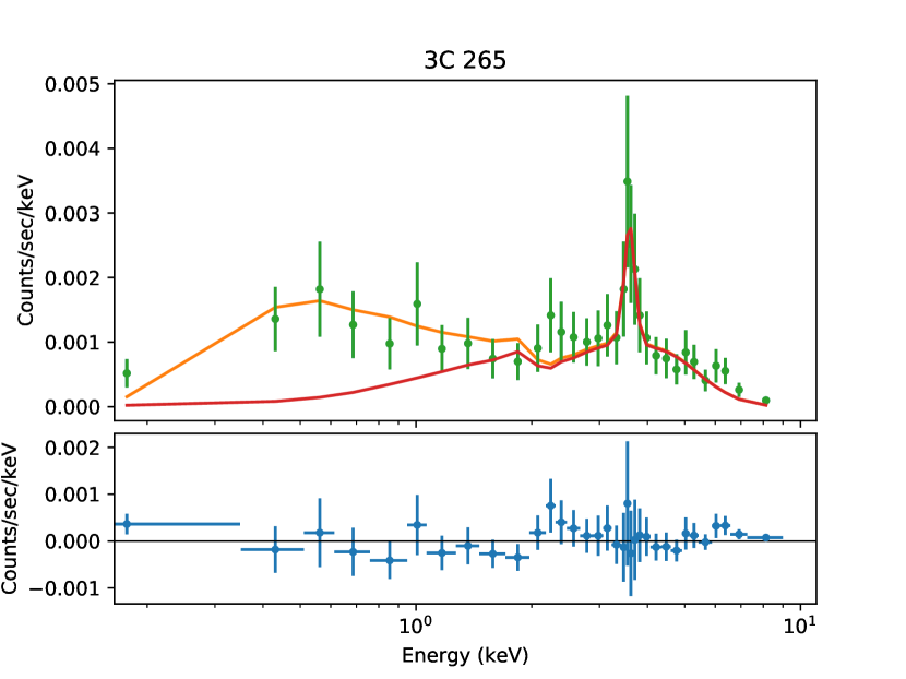
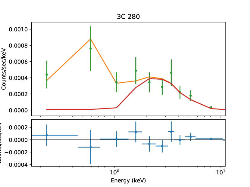
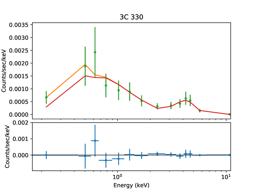
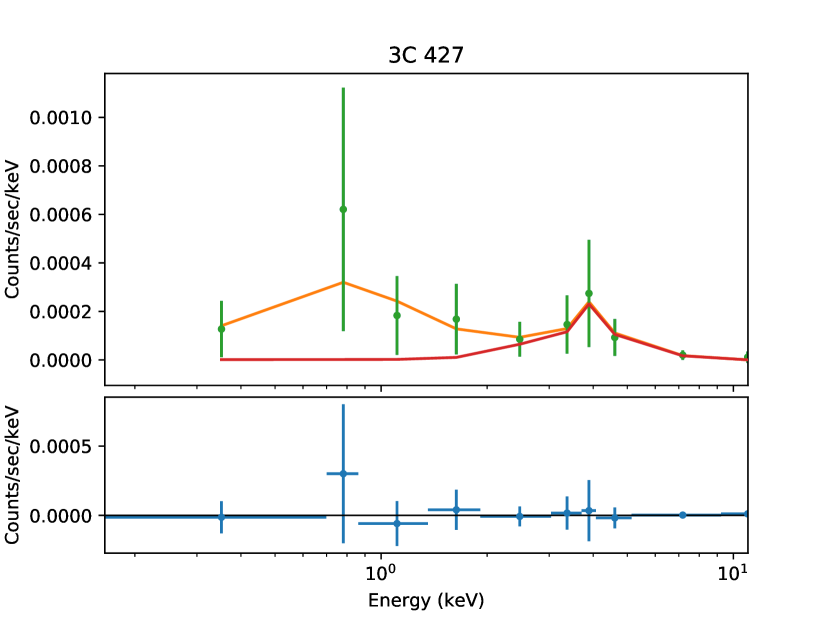
Figure 2: Sherpa X–ray fits (yellow line) to sources with complex spectra (in observed frame) modeled with a power-law ($\Gamma=1.9$) absorbed by Galactic and intrinsic $N_{\rm H}$, Fe K$\alpha$ line, and a soft excess modeled as an unobscured power-law ($\Gamma>1.9$ - see Table 3) in 3C 265, 280, 330, 427.1 where also a fit without the soft excess is shown in red. Fit parameters are given in Table 2 and 3. Residuals to the fits are shown in the bottom panel of each figure.

The fits of complex spectra were built up using an iterative approach. In the initial stage, a model consisting of an absorbed power-law was fitted as described in Section 4.3. If an Fe K$\alpha$ line was visible in the fit residuals, the power-law was then fitted over the energy range excluding the line. Next the fitted parameters were frozen, and an additional component, the soft excess or the Fe K$\alpha$ line, was added to the model. For two sources that required both the Fe K$\alpha$ line and the soft excess, the soft excess component was added and fitted first. The soft excess was modeled as an unabsorbed power-law with a fixed $\Gamma=1.9$. Then the slope was freed and fitted, after which the primary, intrinsic power-law normalization and $N_{\rm H}$ were freed and fitted. The Fe K$\alpha$ line was modeled with a Gaussian and fitted iteratively. First the Fe K$\alpha$ line amplitude was fitted assuming an approximate peak position at 6.4 keV (restframe), appropriate for neutral Fe K$\alpha$, and an arbitrary full width at half maximum (FWHM) of 0.2 keV. Then the line amplitude and FWHM were freed and fitted simultaneously. For 3C 265, where the iron line is particularly strong, the position of Fe K$\alpha$ peak was also fitted. As a next step, the Fe K$\alpha$ line parameters were frozen, and all other non-iron parameters (i.e., intrinsic power-law normalization, $N_{\rm H}$, soft excess power-law slope and normalization) were refitted followed by another Fe K$\alpha$ line-only fit. The resulting best-fit parameters for the soft excess and the Fe K$\alpha$ line (in the complex spectra) are given in Table 3. For pileup sources, the pileup fraction is also shown in this table. Spectral fits for all complex sources are plotted in Figure 2.

4.5 Intrinsic $N_{\rm H}$ and $L_{\rm X}$  estimation from Hierarchical Bayesian Model

Here we explore the Hierarchical Bayesian Modeling (hereafter HBM), to constrain individual and whole-sample intrinsic luminosities and column densities and the obscured and Compton-thick AGN fractions in the sample. HBM is a statistical method that facilitates inferences about a population based on individual objects and their observations (and vice versa). Our hierarchical model has three layers: The bottom layer is formed by the observed data (X-ray spectra) and is fixed. The middle layer contains the parameters for each object, namely their intrinsic X-ray luminosity $L$(0.5–10 keV) and column density $N_{\rm H}$. The top layer describes the $L$(0.5–10 keV) and $N_{\rm H}$ distributions of the whole population. The HBM simultaneously finds posteriors on individual and population parameters. It “shrinks” individual parameter estimates toward the population mean, which lowers RMS errors and naturally deals with large uncertainties and upper limits. The uncertainty is determined via nested sampling. The Appendix presents a detailed explanation of the method.

To apply HBM to our sample, we first used Bayesian inference in analyzing the X-ray spectra assuming flat, uninformative priors for $L$(0.5–10 keV) and $N_{\rm H}$, which were then updated using Bayes’ theorem to posterior priors taking into account parameter distributions of the whole population. The Bayesian X-ray Analysis module was used (BXA; Buchner et al., 2014) for Sherpa (Fruscione et al., 2006), assuming an AGN with intrinsic obscuration and taking into account Compton scattering and iron fluorescence (BNTORUS model; Brightman & Nandra, 2011) with an added warm-mirror power-law (same as the scatterd light component in Section 4.4). All normalizations had wide log-uniform priors, and the intrinsic photon index was assigned a Gaussian prior centered at $1.95$ with standard deviation of $0.15$. The warm-mirror normalization can reach up to $10\%$ of the intrinsic AGN power-law component. The above setup is described e.g., by Buchner et al. (2014). The analysis gives preliminary posterior probability distributions for the parameters in the middle layer, i.e., the individual posterior HBM $L$(0.5–10 keV) and $N_{\rm H}$, which are shown in Figures 3, 4, and 5. The effect of the HBM is that weak observations are informed by well-constrained observations, which indicate probable parameter values. For example, extremely high luminosities are suppressed. The HBM median values of intrinsic $L$(0.5–10 keV) and $N_{\rm H}$ for each source are given in Table 4.

5 Comparison of X-ray Properties of quasars and NLRGs

5.1 Observed X-ray luminosity and Hardness Ratio

The quasars and NLRGs in the medium-$z$ 3CRR sample have comparable (to within $\sim$1.5 dex) extended 178 MHz radio luminosities (Section 2, Figure 1 left) which implies similar intrinsic AGN luminosities. In contrast, the 2$-$8 keV luminosities, uncorrected for intrinsic absorption, hardly overlap (Figure 1 right), where the NLRGs show 10–1000 times lower hard-X-ray luminosities than quasars, suggesting higher obscuration in NLRGs. The widely different apparent luminosities are consistent with the Unification model, where the nuclei of NLRGs are thought to be viewed edge-on through a dusty, torus-like structure and so are observed through higher amounts of obscuration than the quasars.

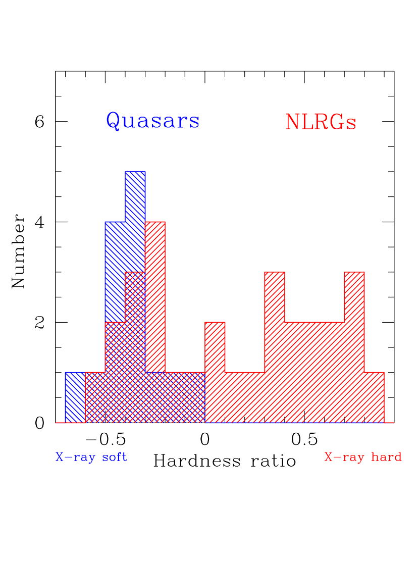
Figure 6: Histograms of the X-ray hardness ratios for quasars (blue) and NLRGs (red). The NLRGs with quasar-like HR $<0$ are: 3C 6.1, 175.1, 220.3, 228, 263.1, 330, 343, 343.1, 455.

The X-ray hardness ratio, defined as ${\rm HR}\equiv\frac{(H-S)}{(H+S)}$, where $H$ and $S$ are the (2$-$8 keV) and (0.5$-$2 keV) counts respectively, is often used as a measure of intrinsic $N_{\rm H}$ and is particularly useful in lower-count sources, where spectral fitting is not possible. Higher (harder) hardness ratio indicates higher obscuration, and lower (softer) hardness ratio lower obscuration. A few sources in our sample have low counts, so we determined the hardness ratios using the Bayesian Estimation of Hardness Ratios (BEHR) method (Park et al., 2006), which accounts for the Poissonian nature of the data and correctly deals with non-Gaussian error propagation, appropriate for both the low- and high-count regimes. These hardness ratios are provided in Table 2 (column 14), and their distribution is presented in Figure 6. All quasars (plotted in blue) have soft HR$<0$, with the mean HR$=-0.36\pm 0.15$, consistent with an AGN power-law with $\Gamma=1.5^{+0.32}_{-0.33}$ and low obscuration. 3C 196, the quasar with the hardest HR ($=-0.07$) in the sample has intermediate obscuration of $N_{\rm H}$$=3\times 10^{22}$ cm^-2 and is classified as a Type 1.8 based on its optical spectrum. In contrast, the NLRGs (plotted in red) span a wide range of hardness ratios $-0.6<HR<0.9$, implying a large range of intrinsic obscuration.

5.2 Hardness Ratio vs. X-ray Absorption

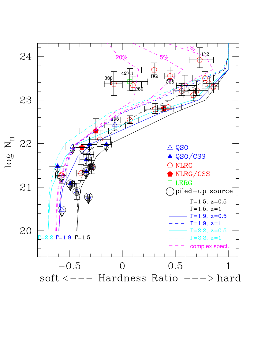
Figure 7: The intrinsic column density $N_{\rm H}$ fitted with Sherpa (available for sources with $>$30 cts) as a function of the observed X-ray hardness ratio (Section 5.1). Lines show the relation between $N_{\rm H}$ and hardness ratio for an absorbed power-law with $\Gamma$ = 1.5 (blue), 1.9 (black), or 2.2 (green) at two values of redshift $z=0.5$ (solid lines) and $z=1$ (dotted lines) spanning the sample’s redshift range. The $N_{\rm H}$ ranges from $10^{20}$ to $10^{25}$ cm^-2. Red dashed lines show the absorbed power-law model with $\Gamma=1.9$ at $z=1$ to which a scattered component was added with a 1%, 5%, and 20% normalization, relative to the intrinsic power-law. This additional component is needed to explain softer hardness ratios in comparison with the model predictions in 3C 172, 184, 265, 280, 330, 427.1 The different symbols indicate the class of source as shown in the legend.

Figure 7 shows the dependence of the observed hardness ratio on $N_{\rm H}$  compared to trends expected from modeling. The intrinsic $N_{\rm H}$ was obtained from X-ray spectral fitting (Sec. 4.3, 4.4) for sources with at least 30 cts. Most of the sources lie on the track of the pure absorbed power-law models with photon index $1.5<\Gamma<2.2$ and $10^{20}<$ $N_{\rm H}$/cm^-2 $<10^{25}$. The exceptions are 3C 172, 184, 265, 280, 330, 427.1, for which the hardness ratios are softer than predicted from an absorbed power-law with the measured $N_{\rm H}$. Apart from 3C 172, for which low $S/N$ (32 cts) does not allow for a complex fit, these are the sources with complex spectra discussed in Section 4.4. These sources’ spectra include an additional soft excess component (besides the heavily obscured power-law and the Fe K$\alpha$ line) which is possibly due to scattered nuclear light or extended X-ray emission from gas surrounding the nucleus, galaxy cluster or the radio/X-ray jet.

The Chandra data of 3C 184 had too few counts ($\sim$48) to justify a complex fit, but the higher $S/N$ XMM-Newton data require a soft excess, high column density ($N_{\rm H}$ $=4.9^{+2.2}_{1.2}\times 10^{23}$ cm^-2), and an Fe K$\alpha$ line (Belsole et al., 2006).

5.3 Hardness Ratio vs. $L_{\rm X}$  Dependence

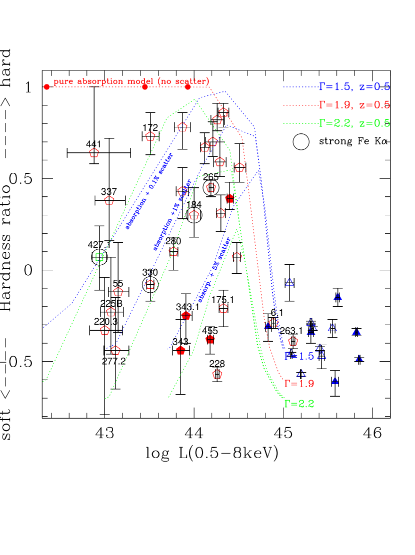
Figure 8: X-ray hardness ratio as a function of 0.5–8 keV X-ray luminosity not corrected for intrinsic absorption. The different symbols indicate the source type and are the same as in Figure 7. Sources with strong iron K$\alpha$ are circled. The red dotted curve shows a power-law model with $\Gamma=1.9$ absorbed by intrinsic column density ranging from $N_{\rm H}$= $1\times 10^{20}$ cm^-2 (lower right corner) to $5\times 10^{24}$ cm^-2 (upper left corner), where large red dots (from right to left) indicate $N_{\rm H}$ = (1,2,5)$\times 10^{24}$ cm^-2. Other dotted curves show absorbed ($N_{\rm H}$ between $1\times 10^{20}-1\times 10^{25}$ cm^-2) power-law models with $\Gamma$ = 1.5 (blue) and $\Gamma$=2.2 (green) with an added scattered light component normalized to 0.1%,1%, and 5% of the intrinsic AGN continuum. All curves are for $z=0.5$. Most NLRGs require an additional, scattered light component.

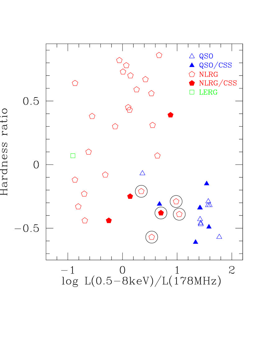
Figure 9: X-ray hardness ratio as a function of the ratio of 0.5$-$8 keV luminosity (uncorrected for intrinsic $N_{\rm H}$) to the total 178 MHz radio luminosity. Symbol shapes indicate object class as in Figure 7. The low-$N_{\rm H}$ NLRGs are circled.

The observed (uncorrected for $N_{\rm H}$) broad-band 0.5–8 keV X-ray luminosities are plotted against hardness ratios in Figure 8. These are compared with a pure absorbed power-law model ($\Gamma=1.9$; red dotted curve), and other absorbed power-law models ($\Gamma=1.5,2.2$) with an added soft excess componenf of varying strength (0.1%, 1%, 5% of intrinsic light; blue and green curves). The quasars have high observed $L_{\rm X}$ and soft hardness ratios indicating low obscuration. The NLRGs show a broad range of hardness ratios and lower observed $L_{\rm X}$, indicating a varying degree of intrinsic $N_{\rm H}$ and varying amount of scattered/extended light emission. The majority of medium-$z$ NLRGs lie on models that include an absorbed power-law and a soft excess of varying strength, which makes their HR softer than the ones expected from a pure absorbed power-law model. Figure 9 is a modified version of Figure 8 where the observed, 0.5–8 keV X-ray luminosity is normalized to the total radio luminosity at 178 MHz (a surrogate for intrinsic AGN luminosity). Quasars show $L$(0.5$-$8 keV)/$L$(178 MHz)$>1$ and soft HR. NLRGs have $L$(0.5$-$8 keV)/$L$(178 MHz)$<1$ and a range of HR. A group of five soft NLRGs (3C 6.1, 175.1, 228, 263.1, 455) has almost quasar-like $L$(0.5$-$8 keV)/$L$(178 MHz) $\sim 1$, indicating low obscuration. These will be discussed further in Sections 6.2 and 6.3.

5.4 Comparison with the high-$z$ 3CRR sample

The mean quasar hardness ratio of the medium-$z$ 3CRR sample ($-$0.36$\pm$0.15) is comparable to that of the high-$z$ 3CRR sample ($-$0.44$\pm$0.20). However, the median is harder ($-$0.34 vs. $-$0.51) implying flatter primary power-law slopes ($\Gamma$=1.5 vs. 1.9) and/or higher $N_{\rm H}$ in the medium-$z$ quasars, which may reflect the fact that low $N_{\rm H}$ is easier to measure at lower redshifts as the softer X-rays move into the Chandra observed band. Piled-up quasars, present at medium-$z$, will also contribute to the harder mean and median hardness ratios. For NLRGs, the mean hardness ratio (0.14$\pm$0.43) is comparable, within uncertainties, to the high-$z$ NLRG mean (0.10$\pm$0.45), while the median is softer (0.10 vs. 0.26) implying a higher fraction of NLRGs with low $N_{\rm H}$ in the medium-$z$ sample (discussed in Section 6.2).

The median 2–8 keV luminosity, uncorrected for intrinsic column density, is 6$\times$ lower for NLRGs than quasars in the medium-$z$ sample (10^44.4 erg s^-1 vs. 10^45.2 erg s^-1 respectively), while it was $\sim 100\times$ lower in the high-$z$ 3CRR sample (Wilkes et al., 2013), suggesting a higher number of NLRGs with low obscuration in the medium-$z$ sample.

6 Discussion

6.1 Orientation-Dependent Obscuration

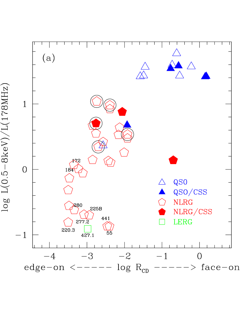
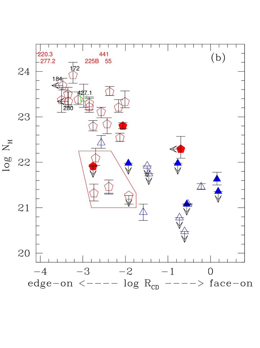
Figure 10: The ratio of 0.5–8 keV luminosity, uncorrected for $N_{\rm H}$, to the total 178 MHz luminosity (left) and intrinsic equivalent hydrogen column density ($N_{\rm H}$, right) estimated from spectral fits as a function of the radio core fraction $R_{\rm CD}$. A strong trend with $R_{\rm CD}$ for both parameters is consistent with the orientation-dependent obscuration of Unification models. Compton-thick sources are named in both figures (however in figure on the right 3C 55, 220.3, 225B, 277.2, 441 with no $N_{\rm H}$ estimate due to low $S/N$ have only their names indicated at their log $R_{\rm CD}$ values and log $N_{\rm H}$/cm${}^{-2}>$24). The low $N_{\rm H}$ NLRGs are circled in figure on the left and enclosed in a red contour in figure on the right. Symbols in both figures indicate source type as in Figure 7.

The ratio of the observed broad-band 0.5–8 keV X-ray luminosity (uncorrected for $N_{\rm H}$) to the total radio luminosity at 178 MHz ($L_{\rm X}/L_{\rm R}$, where $L_{\rm R}=\nu L_{\nu}(178\,{\rm MHz})$ is calculated from the 178 MHz flux densities in Laing et al., 1983), which is a measure of gas obscuration, is plotted in Figure 10a as a function of the radio core fraction $R_{\rm CD}$ (an orientation indicator). Sources with lower obscuration have higher $L_{\rm X}/L_{\rm R}$ ratios and show larger values of $R_{\rm CD}$, i.e., are preferentially seen at lower viewing angles in respect to the radio jet (i.e., face-on to the torus). Sources with higher obscuration (lower $L_{\rm X}/L_{\rm R}$) have lower $R_{\rm CD}$ and so are preferentially viewed perpendicular to the radio jet (i.e., edge-on to the torus). To show this explicitly, the intrinsic column density $N_{\rm H}$ (estimated from X-ray spectral fits in Sec. 4.3  and 4.4), is plotted as a function of the radio core fraction $R_{\rm CD}$ in Figure 10 b. The strong relation between $N_{\rm H}$ (and $L_{\rm X}/L_{\rm R}$) and $R_{\rm CD}$ implies that obscuration is strongly dependent on orientation and increases with increasing viewing angle. This relation is consistent with the orientation-dependent obscuration invoked by the Unification model and agrees with our results for the high-$z$ 3CRR sample (Wilkes et al., 2013). However, at intermediate viewing angles $-3<\log$ $R_{\rm CD}$ $<-2$ NLRGs with a broad range of $N_{\rm H}$ exist. These include typical, obscured NLRGs with $N_{\rm H}$ $>10^{22}$ cm^-2 and a peculiar class of NLRGs, not present in the high-$z$ 3CRR sample, with low intrinsic column densities $N_{\rm H}$ $\lesssim$$10^{22}$ cm^-2. These low-$N_{\rm H}$ NLRGs cannot be explained by a simple Unification model dependent solely on orientation, and suggest that a second parameter (clumpy torus, different obscurer, or different $L/L_{\rm Edd}$ ratio) is needed. We will focus on the low-$N_{\rm H}$ NLRGs next.

6.2 Observational properties of low-$N_{\rm H}$ NLRGs

One quarter of NLRGs (3C 6.1, 175.1, 228, 263.1, 455), or 14% of the medium-$z$ 3CRR sample, have low $N_{\rm H}$ ($10^{21}-10^{22}$ cm^-2), similar to the unobscured BLRGs and quasars. As a result of low obscuration, these NLRGs have soft, quasar-like hardness ratios ($HR<0$) and the highest $L_{\rm X}/L_{\rm R}$ amongst the NLRGs (Figure 10 a). These low-$N_{\rm H}$ NLRGs have intermediate core fractions ($-2.7<$ log $R_{\rm CD}$ $<-2$) and so are likely viewed at angles skimming the edge of the accretion disk or torus. No such sources were present in the high-redshift 3CRR sample, where all NLRGs had higher intrinsic column densities of log $N_{\rm H}$/cm^-2 $>22.7$ and log $R_{\rm CD}$ $<-2$. Although it is easier to measure low $N_{\rm H}$ values in sources at medium-$z$ than at high-$z$ (as the softer-energy X-rays move into the Chandra-observed band), the spectra also become more complex, often including an additional, soft excess component. The low-$N_{\rm H}$ NLRGs have enough counts (90–1700) to model the soft excess, but none of them required one. We hence conclude that the low intrinsic column densities in these NLRGs are measured correctly and are not underestimated due to the lack of soft excess modeling in low-$S/N$ spectra.

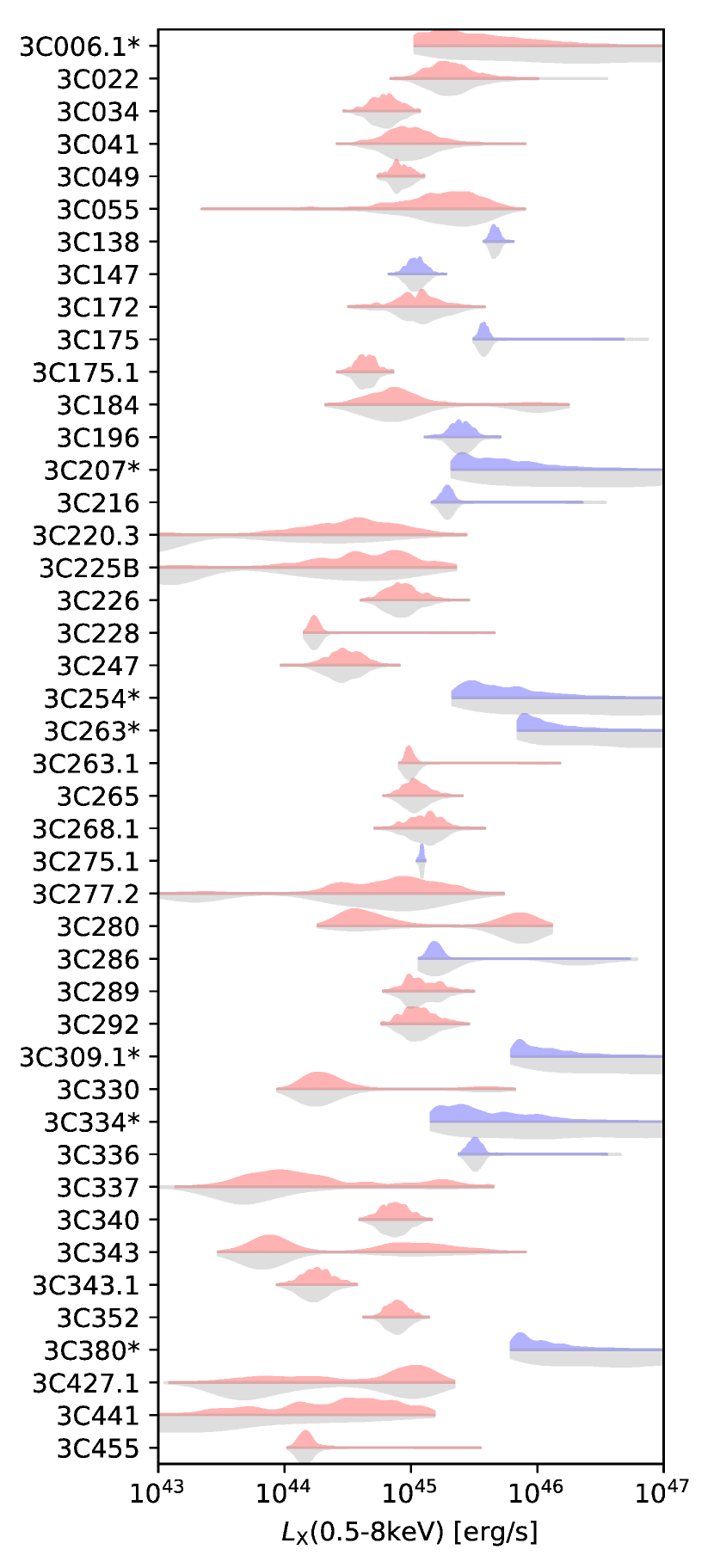
Figure 4: Constraints on the intrinsic 0.5$-$8 keV X-ray luminosity for each source in the sample from the Hierarchical Bayesian Modeling. Gray distributions show probabilities when assuming (as a first step of the HBM) flat, uninformative priors. Results with posterior probabilities (after incorporating information from the whole sample) are shown in blue for quasars and in red for NLRGs. Thicker vertical dimension of contours implies higher probability. Sources with substantial pileup are marked with an asterisk.

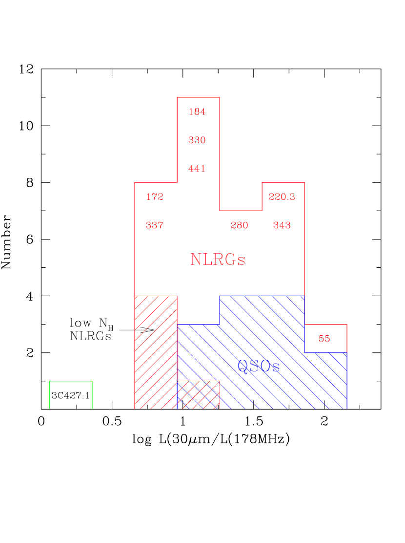
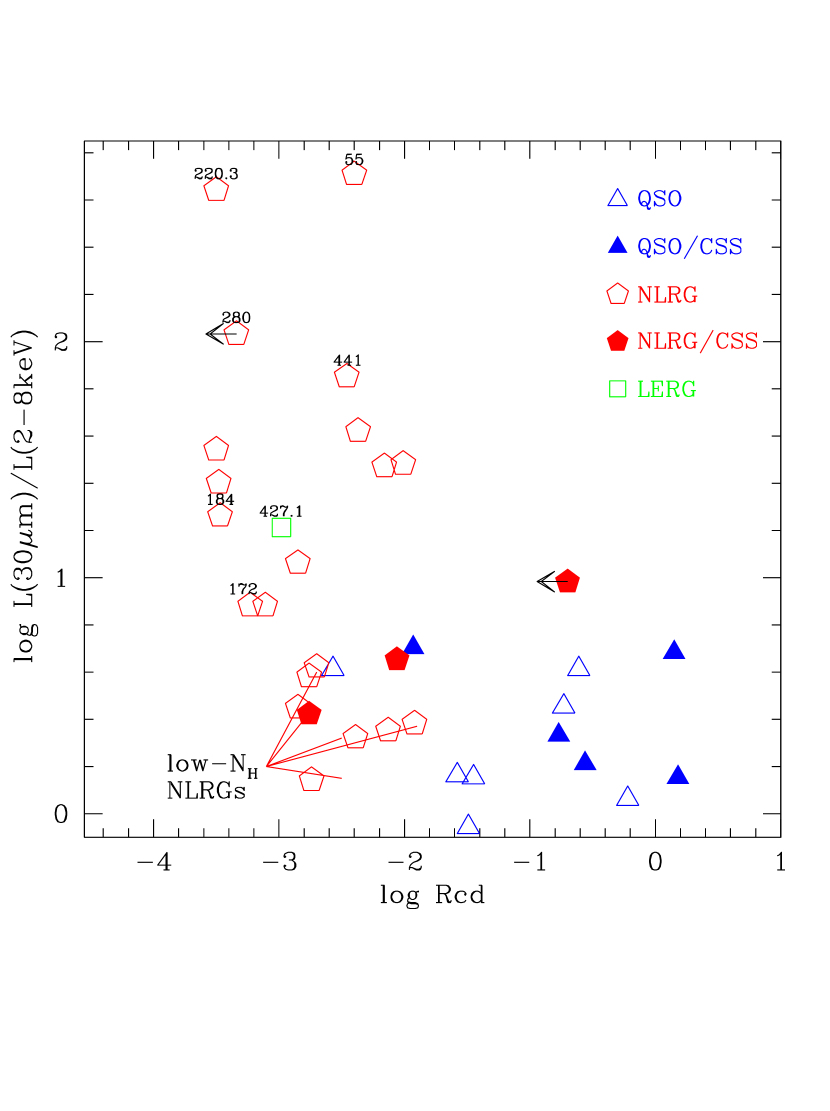
Figure 11: (Left:) Histogram of the 30 $\mu$m to 178 MHz luminosity ratios. Quasars are plotted in blue and NLRGs in red. The low-$N_{\rm H}$ NLRGs are shown by the red hatched histogram. 3C 427.1, plotted in green, has low MIR emission, as expected for LERGs (Westhues et al., 2016). Compton-thick and borderline Compton-thick sources are indicated by their 3C identification. (Right:) The ratio of 30 $\mu$m to 2-8 keV luminosity (not corrected for $N_{\rm H}$) as a function of the radio core fraction $R_{\rm CD}$. Different symbols indicate source type as in Figure 7. The Compton-thick sources are named and NLRGs with low $N_{\rm H}$ are indicated in both figures.

The low-$N_{\rm H}$ NLRGs show relatively low mid-IR (30$\mu$m) emission when compared to their radio emission. The $L$(30 $\mu$m)/$L$(178 MHz) ratios are the lowest in the sample (Figure 11 a), $\sim$10 times lower than in quasars. Because the X-ray emission is also weaker by a factor of 10 relative to radio emission (see Figure 10 a), the $L$(30 $\mu$m)/$L$(2$-$8 keV) ratios are comparable to those of quasars (see Figure 11 b). The spectral energy distributions (SEDs) of low-$N_{\rm H}$ NLRGs show no infrared or big blue bump (see Figures 4, 5, 7 of Westhues et al., 2016), and the specific star formation rates are close to those of normal galaxies (Westhues et al., 2016).

Three of the low-$N_{\rm H}$ NLRGs were observed with HST (3C 6.1, 228, 263.1). The optical images show compact host galaxies with no visible dust lanes (McCarthy et al., 1997). The optical SDSS spectra are red (3C 175.1, 228, 263.1, 455). 3C 6.1 shows a weak optical continuum dominated by the host galaxy (visible $\lambda$4000Å absorption feature) with an 8 Gyr old stellar population (Smith et al., 1979). 3C 455 has conflicting optical types (Type 1 or 2) in the literature, but we classify this source as a Type 2 based on the spectrum presented by Gelderman & Whittle (1994), which shows a weak continuum and no broad H$\beta$ emission line. H$\alpha$, however, was not covered to check for intermediate Type 1.8 or 1.9.

6.3 Understanding the low-$N_{\rm H}$ NLRGs

Possible scenarios that can explain low column densities, lack of broad emission lines, and weak IR emission in the low-$N_{\rm H}$ NLRGs are the following:

• These are “true” type 2 objects (Panessa & Bassani, 2002; Tran, 2003; Shi et al., 2010; Merloni et al., 2014), which show no detectable broad lines and have low X-ray absorption. In such sources the broad line region (BLR) has faded due to recent weakening of the continuum or has not formed due to very low $L/L_{\rm Edd}$ $\ll 10^{-2}$ (Nicastro, 2000). In the latter scenario, such low $L/L_{\rm Edd}$ ratios would result in more than $100-1000\times$ weaker 0.5–8 keV luminosities (as accretion disk SEDs strongly depend on $L/L_{\rm Edd}$ – see e.g., Czerny et al., 1996, Fig. 1), but the values of $L_{\rm X}/L_{\rm R}$ only few-to-$10\times$ lower than in quasars (Figure 10 a) rule out this scenario.

• The obscuration is non-standard, caused not by a torus but by a dust lane or a host galaxy disk mis-aligned with the dusty torus (as in the red 2MASS AGN; Kuraszkiewicz et al., 2009a, b) which would result in $N_{\rm H}$ $\leq 10^{22}$ cm^-2. Such column density is low enough not to obscure significantly the intrinsic X-ray emission or the IR emission from the dusty torus, but is sufficient to hide the AGN’s optical+UV continuum and the broad emission line region. In this scenario, the weak IR emission in low-$N_{\rm H}$ NLRGs cannot be easily explained unless the dusty torus is absent.

• Low $L/L_{\rm Edd}$ ratio. The low-$N_{\rm H}$ NLRGs are found at intermediate viewing angles ($-3<$ log $R_{\rm CD}$ $<-2$), together with NLRGs that have higher column densities of $10^{22.5}<$ $N_{\rm H}$/cm^-2 $<10^{23.5}$ (Figure 10 b). Therefore, a scenario is needed in which clouds with a large range of column densities may exist at such viewing angles. Fabian et al. (2008) showed that the distribution of column densities of the gas and dust clouds surrounding an AGN is a function of $L/L_{\rm Edd}$, and only clouds with $N_{\rm H}$/cm^-2  $\geq 5\times 10^{23}\times$ $L/L_{\rm Edd}$ can withstand the AGN’s radiation pressure, while the lower-$N_{\rm H}$ clouds are blown away. At low $L/L_{\rm Edd}\sim 0.01$, clouds with column densities ranging from $\sim 10^{22}$ cm^-2 to Compton-thick can exist, whereas at high $L/L_{\rm Edd}\sim 1$, only those with Compton-thick column densities will survive. Applying the scenario to our sample, the NLRGs with low $N_{\rm H}$ must have low $L/L_{\rm Edd}$, while NLRGs with high $N_{\rm H}$ (viewed at similar, intermediate angles) have high $L/L_{\rm Edd}$. The scenario is further confirmed by the finding that the X-ray luminosities, uncorrected for intrinsic absorption, are comparable for the low-$N_{\rm H}$ and high-$N_{\rm H}$ NLRGs having the same intermediate viewing angles ($0.2<L$(0.5$-$8 keV)/$L$(178 MHz)$<1$; Figure 10 a), despite significantly different column densities. Thus we conclude that indeed the low-$N_{\rm H}$ NLRGs have lower intrinsic X-ray luminosities and hence lower $L/L_{\rm Edd}$ than the high-$N_{\rm H}$ NLRGs.

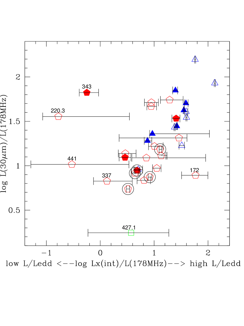
Figure 12: The dependence of the 30 $\mu$m on the intrinsic X-ray emission (from HBM modelling) both normalized to 178 MHz luminosity. The intrinsic X-ray luminosity depends on $L/L_{\rm Edd}$. Symbols indicate source type as in Figure 7. Most quasars and NLRGs follow a strong correlation where the mid-IR increases with intrinsic $L_{\rm X}$ i.e., $L/L_{\rm Edd}$. The outliers are: 3C 220.3 which lenses a background submm galaxy resulting in a higher than expected 30 $\mu$m luminosity, 3C 343 possibly another lens candidate, 3C 172, 441 IR-weak, Compton-thick sources, 3C 427.1 a LERG expected to have low IR emission, and 3C 337 a highly obscured source with low $L/L_{\rm Edd}$ (Sections 6.3, 6.4.2). Low-$N_{\rm H}$ NLRGs are circled in black and show preferably lower mid-IR emission and $L/L_{\rm Edd}$ ratios.

• Weak IR emission due to low $L/L_{\rm Edd}$. At high $L/L_{\rm Edd}$ (strong big blue bump), only a torus that is compact and Compton-thick can withstand the intense UV radiation and strong winds. Dust in such a compact geometry will strongly radiate in the near-to-mid-IR, producing an SED with a strong IR bump (Pier & Krolik, 1992). At lower $L/L_{\rm Edd}$, where the big blue bump is weaker and provides less illuminating flux for the torus, the torus may become clumpy and extended, resulting in a weaker IR bump (Siebenmorgen et al., 2015; Hönig et al., 2010; Nenkova et al., 2008a, b; Kuraszkiewicz et al., 2003). Figure 12 shows the dependence of the 30 $\mu$m luminosity on the 2–8 keV intrinsic luminosity (estimated from the HBM model), which is related to the $L/L_{\rm Edd}$ ratio (e.g., Czerny et al., 1996 Fig. 1). Both luminosities are normalized by the extended radio luminosity $L$(178 MHz) to remove any redshift dependence on the IR and X-ray luminosities. There is a strong correlation between $L$(30 $\mu$m)/$L$(178 MHz) and $L$(2–8 keV)/$L$(178 MHz) with a probability 0.01% of occurring by chance in both the generalized Kendall rank and Spearman rank tests. The correlation indicates that higher $L/L_{\rm Edd}$ sources (=higher intrinsic $L$(2$-$8 keV)) have stronger mid-IR luminosities. The low-$N_{\rm H}$ NLRGs have relatively low $L/L_{\rm Edd}$ (i.e., $L$(2$-$8 keV)/$L$(178 MHz) $<1$) and so their weak mid-IR emission can be explained as due to low $L/L_{\rm Edd}$.

  Two sources, 3C 220.3 and 3C 343, do not lie on the overall correlation in Figure 12. They have relatively low $L/L_{\rm Edd}$ but show strong mid-IR emission. 3C 220.3 is lensing a background submm galaxy (Haas et al., 2014), which results in amplification of its IR luminosity. We suggest that perhaps 3C 343 may also be lensing a background galaxy. Another outlier is 3C 172, with high $L/L_{\rm Edd}$ and low mid-IR emission. The low IR emission can be explained by either extreme Compton-thick obscuration of $N_{\rm H}$ $>10^{25}$ cm^-2 or low amounts of dust due to 1000$\times$ lower than Galactic dust-to-gas ratio. The former explanation is not suported by our low $S/N$ X-ray spectral modeling, which gives $N_{\rm H}$ $\sim 10^{24}$ cm^-2. The latter is in conflict with typical AGN dust-to-gas ratios which are 1–100 times lower than Galactic (Maiolino et al., 2001; Marchese et al., 2012; Burtscher et al., 2016) with a few exceptions having this ratio a few times higher (Ordovás-Pascual et al., 2017; Trippe et al., 2010).

In summary, a simple Unification model where obscuration changes only with orientation cannot fully describe the observed multiwavelength properties of the medium-$z$ 3CRR sample, and a range of $L/L_{\rm Edd}$ ratios, extending to low values, is required to explain the existence and the properties of the low-$N_{\rm H}$ NLRGs. In contrast, the multiwavelength properties of the high-$z$ 3CRR sample were explained by pure Unification, suggesting that $L/L_{\rm Edd}$ had a narrower range and possibly higher values in comparison with the medium-$z$ sample, allowing orientation effects to dominate the observed properties of the sample.

6.4 Heavily obscured NLRGs

6.4.1 Compton-thick (CT) candidates

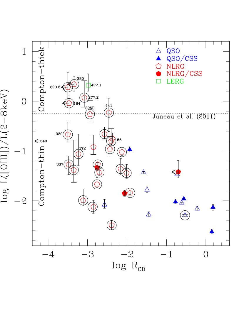
Figure 13: The ratio of L([O iii]) to the 2$-$8 keV X-ray luminosity (not corrected for obscuration) as a function of radio core fraction $R_{\rm CD}$. Symbols indicate source type as in Figure 7. For sources lacking [O iii] measurements, values were estimated from [O ii] measurements following Grimes et al. (2004) and are circled. 3C 427.1 and 3C 292 have [O iii] estimated from 151 MHz radio luminosity. The dotted line is the dividing line between Compton-thin and Compton-thick sources reported by (Juneau et al., 2011). Compton-thick and borderline CT sources are indicated by their 3C identification.

The luminosity of the [O iii]$\lambda$5007 emission line (hereafter $L$([O iii]) was found to track the radio and intrinsic X-ray luminosities for both the Type 1 and Type 2 AGN (Jackson & Rawlings, 1997; Mulchaey et al., 1994). It is often used as an indicator of intrinsic AGN luminosity (Risaliti et al., 1999; Panessa et al., 2006) and has little or no inclination dependence at high luminosities (Grimes et al., 2004; Jackson & Rawlings, 1997). The observed hard X-ray luminosity, on the other hand, is strongly dependent on obscuration (especially at high $N_{\rm H}$), so the ratio of $L$([O iii])/$L$(2–8 keV) is often used to discriminate between Compton-thin and Compton-thick (hereafter CT) sources (Risaliti et al., 1999; Panessa et al., 2006). Figure 13 shows the ratio $L$([O iii])/$L$(2–8 keV) plotted against the radio core fraction $R_{\rm CD}$. The $L$([O iii]) values are from Grimes et al. (2004) and are shown in Table1. Seventeen sources have actual [O iii] measurements, and for the remainder $L$([O iii]) was estimated from either the [O ii]$\lambda$3727 emission line or the 151 MHz radio luminosity (3C 292, 427.1). The dotted line in Figure 13, shows the dividing line between Compton-thin and CT sources reported by Juneau et al. (2011) and seven sources: 3C 184, 220.3, 225B, 277.2, 280, 441 (all NLRGs, with L([O iii]) estimated from L([O ii])) and 3C 427.1 (a LERG) appear to be CT. The HBM analysis (Section 4.5, Table 4, Figure 3) gives CT probabilities ranging from 24%–80%. 3C 220.3, 225B, 277.2, 441 have too few counts ($<15$) to model the X-ray spectrum to confirm the high $N_{\rm H}$, but HBM implies CT obscuration (see Figure 3, Table 4). The low-$S/N$ Chandra spectrum of 3C 184 (48 cts) shows a strong Fe K$\alpha$ line (Figure 2), implying heavy obscuration (the reflection component becomes stronger as the intrinsic power-law weakens with increasing obscuration), while the higher-$S/N$ XMM data are fitted with high $N_{\rm H}$, strong K$\alpha$ line, and a soft excess (Belsole et al., 2006). The Chandra X-ray spectrum of 3C 280 (117 counts) is modeled with a strong soft excess and intermediate $N_{\rm H}$ (Figure 2, Table 2).

Five of the above CT candidates have measured $L$(30 $\mu$m) (Westhues et al., 2016) and all except 3C 427.1 have log $L$(30 $\mu$m)/$L$(2–8 keV) $>1.8$ (Figure 11b). The Spitzer/IRS spectra of 3C 184 and 3C 441 show strong 9.7 $\mu$m silicate absorption (an indicator of large amounts of dust) with $\tau_{\rm 9.7}$ $>0.3$. 3C 280, despite being a CT candidate, has no 9.7 $\mu$m silicate absorption (Georgantopoulos et al., 2011). All the above CT candidates, except for 3C 427.1, have log $R_{\rm CD}$ $<-3$ indicating inclination angles larger than 80° (i.e., orientation edge-on to the torus).

For 3C 427.1, neither the [O iii] nor [O ii] luminosity was measured directly, and $L$(151 MHz) was used to estimate $L$([O iii]). To confirm this source’s CT nature we consider other CT indicators. 3C 427.1 has the lowest $L$(0.5$-$8 keV)/$L$(178 MHz) in the sample (Figure 10a) suggesting low observed $L_{\rm X}$, which may be either due to CT obscuration, low $L/L_{\rm Edd}$, or X-rays being recently turned off (the source is a LERG which harbors a low luminosity AGN). The $L$(30 $\mu$m)/$L$(178 MHz) ratio is the lowest in the sample (Figure 11a). Low mid-IR emission is typical for LERGs (Westhues et al., 2016), where low $L/L_{\rm Edd}$ results in weaker big blue bump emission, which provide less illuminating flux for the circumnuclear dust emitting in the IR (Figure 12 shows the dependence between $L/L_{\rm Edd}$ and $L$(30 $\mu$m)/$L$(178 MHz)). Alternatively the mid-IR emission could be suppressed by heavy obscuration, $N_{\rm H}$ $\gtrsim 10^{25}$ cm^-2, resulting in a strong 9.7 $\mu$m silicate absorption which cannot be checked in the source for lack of a Spitzer/IRS spectrum. However, the presence of a strong Fe K$\alpha$ line (Figure 2) implies that 3C 427.1 is indeed heavily obscured.

6.4.2 CT and borderline CT candidates with low [OIII] emission

There are five NLRGs that have low $R_{\rm CD}$ values implying extreme (edge-on) inclination angles characteristic of the CT sources described above but having low, Compton-thin $L$([O iii])/$L$(2–8 keV) ratios. Despite this, these sources are possibly CT or borderline CT as explained below:

3C 55: Sherpa modeling of the 15-count Chandra spectrum does not give an estimate of intrinsic $N_{\rm H}$, but HBM finds CT $N_{\rm H}$ and a 97% probability of the source being CT (Table 4). The Spitzer/IRS spectrum shows strong 9.7 $\mu$m silicate absorption indicating heavy absorption. Also the $L$(30 $\mu$m)/$L$(2$-$8 keV) and $L$(0.5$-$8 keV)/$L$(151 MHz) ratios have values consistent with other CT sources in the sample. The source is definitely CT.

3C 172: both Sherpa modeling of the 30-count X-ray spectrum and HBM imply $N_{\rm H}$ consistent with CT (Table 2 and 4) with a 52% probability of being CT. This strong CT candidate is unusually weak in the IR (Figure 11a), having no Herschel detection, and showing an SED with no IR bump (Westhues et al., 2016). No Spitzer/IRS spectrum is available to estimate the strength of the 9.7 $\mu$m silicate absorption.

3C 330: the X-ray spectrum (143 counts) is modeled with a highly absorbed (but not CT) power-law (Table 2) and includes a soft excess and medium strength iron K$\alpha$ line (Figure 2). HBM estimates a high but not CT $N_{\rm H}$ and a 9% CT probability (Table 4). The Spitzer/IRS spectrum shows a moderate 9.7 $\mu$m silicate absorption (Westhues et al., 2016). The source is definitely heavily obscured but not CT.

3C 337: the low-$S/N$ spectrum (10 counts) does not allow for an $N_{\rm H}$ estimate from Sherpa modeling. HBM gives an estimate of high but not CT obscuration and a 13% probability that this source is CT (Table 4). No Spitzer/IRS spectrum is available to estimate the strength of the silicate 9.7 $\mu$m absorption. The $L$(30 $\mu$m)/$L$(2$-$8 keV) is in the range of highly obscured sources (Figure 11b). 3C 337 is weak in the mid-IR, having one of the lowest $L$(30 $\mu$m)/$L$(178 MHz) ratios in the sample (Figure 11a) implying low $L/L_{\rm Edd}$ (Figure 12). The intrinsic hard X-ray luminosity estimated from HBM (Table 4) is also one of the lowest in the sample, suggesting low $L/L_{\rm Edd}$. The source has low $L$(0.5$-$8 keV)/$L$(178 MHz) and $L$(2$-$8 keV)/$L$(178 MHz) values within the range of CT sources (Figure 10a). 3C 337 is heavily obscured but not CT.

3C 343 was classified in NED as a quasar (Spinrad et al., 1985; Baldwin et al., 1973), but Aldcroft et al. (1994) reclassified this source as a Type 2 based on an optical spectrum that lacks a broad H$\beta$ emission line (although H$\alpha$ was not covered). Also Lawrence et al. (1996) found only narrow Mg ii and C iv emission lines in their spectra. The low $L$(2$-$8 keV)/$L$(178MHz) and $L$(0.5–8 keV)/$L$(178 MHz) are in the range of other CT candidates in the sample (Fig. 10a). The log $L$(30 $\mu$m)/$L$(2$-$8 keV) and log $L$(30 $\mu$m)/$L$(178 MHz) are also consistent with other CT candidates. Strong 9.7 $\mu$m silicate absorption, visible in the IRS/Spitzer spectrum (Westhues et al., 2016) implies heavy dust obscuration. Contrary to these CT indicators, $L$([O iii])/$L$(2–8 keV) lies below the CT line (Figure 13). The low $L(\hbox{\sc[O~{}iii]})$ was measured directly (Grimes et al., 2004). 3C 343 is a CSS source, where the radio jets are thought to be young or frustrated by large amounts of material. In the latter case, the ionizing photons could be trapped by the dense material that is frustrating the jets, resulting in low [OIII] emission and a Compton-thin $L$([O iii])/$L$(2$-$8 keV) ratio. The X-ray spectrum has too few counts (18-cts) to estimate $N_{\rm H}$, but HBM gives a non-CT $N_{\rm H}$, one of the lowest intrinsic X-ray luminosities in the sample (possibly implying low $L/L_{\rm Edd}$), and a 14% probability that this source is CT (Table 4). We conclude 3C 343 is heavily obscured but likely not CT.

Based on our multiwavelength analysis we find nine CT AGN (3C 55, 172, 184, 220.3, 225B, 277.2, 280, 427.1, 441) and three (3C 330, 337, 343) heavily obscured but not CT objects in the medium-redshift 3CRR sample. We conclude that 20% of the sources in this sample are CT, consistent with the 21% found for the high-$z$ 3CRR sample (Wilkes et al., 2013).

6.5 Reliability of Compton-thick indicators

Table 5 summarizes the various CT indicators for each of the CT candidates discussed above and shows that these indicators do not always agree. We analyze the reasons and give recommendations for their use.

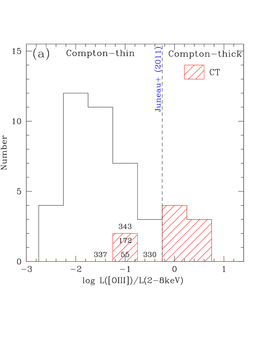
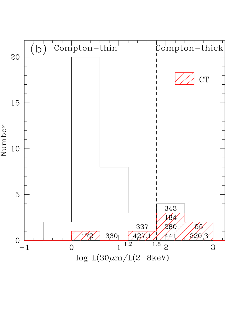
Figure 14: Histograms of high obscuration indicators: the ratio of [O iii]$\lambda$5007 to the observed 2$-$8 keV X-ray luminosity (left) and 30 $\mu$m to the observed 2–8 keV luminosity (right). The 2$-$8 keV X-ray luminosities are uncorrected for intrinsic $N_{\rm H}$. Compton-thick sources are denoted by the red hatched regions. The L([O iii])/L(2–8 keV)$\geq-0.25$ value from Juneau et al. (2011) (dashed line) finds exclusively CT sources, but misses 3C 55 and 3C 172. The $L$(30 $\mu$m)/$L$(2–8 keV)$>1.8$ ratio finds most Compton-thick sources except for 3C 172 and 3C 427.1.

The distribution of the most widely used CT indicator $L$([O iii])/$L$(2$-$8 keV), where $L$(2$-$8 keV) is X-ray luminosity not corrected for intrinsic $N_{\rm H}$, is plotted in Figure 14a. Most (7/9=78%) of the CT candidates in our medium-$z$ 3CRR sample lie at log $L$([O iii])/$L$(2$-$8 keV)$\geq-0.25$ the dividing line between the Compton-thin and CT sources from (Juneau et al., 2011). Exceptions are 3C 55, 172, which together with the three borderline CT sources (3C 330, 337, 343) show Compton-thin $L$([O iii])/$L$(2$-$8 keV). Interestingly, sources that make the CT cut cover a full range of sample’s intrinsic $L_{\rm X}$ (log $L_{\rm X}$ $=43-46$ - see Table 4) which means that they also cover the full range of $L/L_{\rm Edd}$ in the sample, suggesting that $L$([O iii])/$L$(2$-$8 keV) is independent of $L/L_{\rm Edd}$.

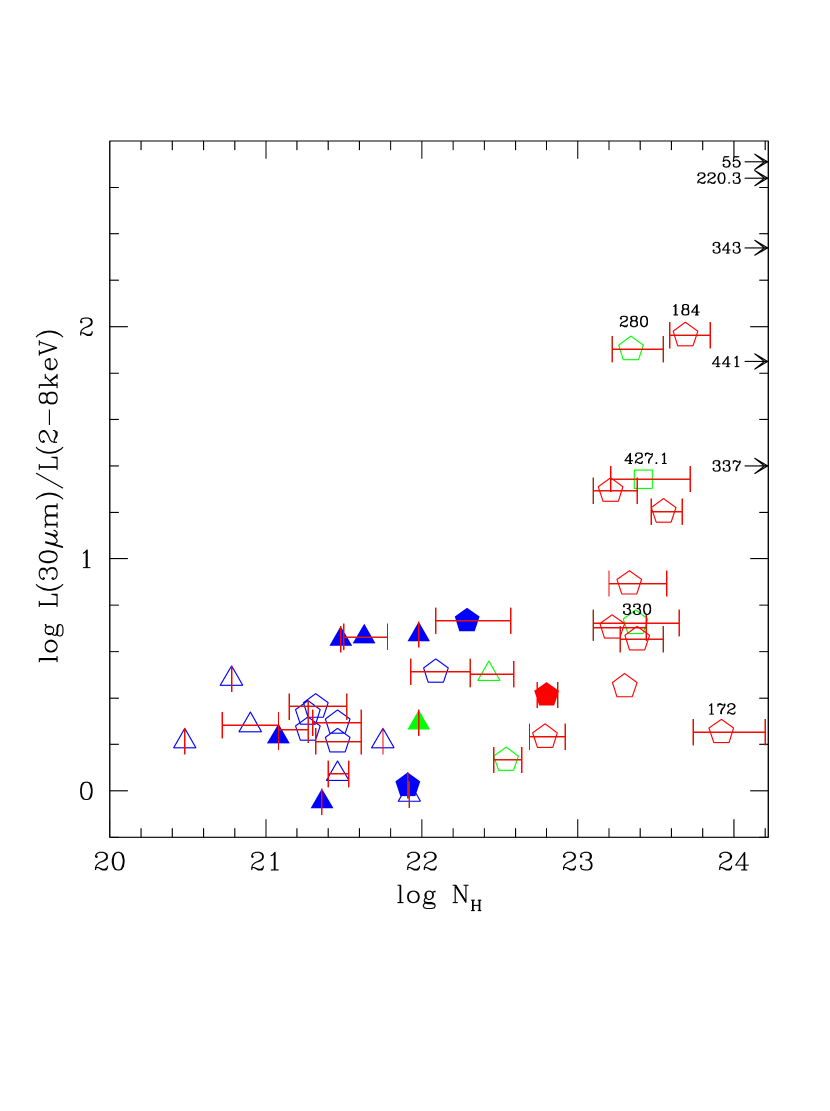
Figure 15: Dependence of the 30 $\mu$m to 2$-$8 keV X-ray (uncorrected for $N_{\rm H}$) luminosity ratio on intrinsic $N_{\rm H}$. For many sources with $N_{\rm H}$ $>10^{23}$ cm^-2 the L(30 $\mu$m)/L(2$-$8 keV) ratio substantially increases above 1. Symbols denote source type as in Figure 7. Compton-thick and borderline Compton-thick sources are labeled. Low $S/N$ Compton-thick sources without an $N_{\rm H}$ estimate (due to low $S/N$) are indicated along the ordinate only by their 3C identification.

The mid-IR (30 $\mu$m) luminosity, similarly to the $L$([O iii]), is used as a measure of intrinsic AGN luminosity, hence $L$(30 $\mu$m)/$L$(2$-$8 keV) can also be used as an indicator of CT obscuration. We plot this ratio as a function of $N_{\rm H}$ in Figure 15 and find that most of the sources with $N_{\rm H}$ $>10^{23}$ cm^-2 have log $L$(30 $\mu$m)/$L$(2–8 keV) $>1$. The distribution of $L$(30 $\mu$m)/$L$(2$-$8 keV) in Figure 14b shows that a value $>1.8$ finds most CT sources in the sample: five out of seven (71%) CT candidates with measured $L$(30 $\mu$m) and one borderline CT source. Relaxing this criterion to $>1.2$ finds 6 out of those 7 CT sources (86%), but also picks three highly obscured, non-CT NLRGs. 3C 172 is the only CT source with log $L$(30 $\mu$m)/$L$(2$-$8 keV) $<1$ due to the unusually weak mid-IR emission (see Section 6.4.2). The $L$(30 $\mu$m)/$L$(2$-$8 keV) $>1.8$ is therefore a robust CT indicator, but it does not find CT sources exclusively. The ratio may be enhanced by emission from lensed background galaxies (as in 3C 220.3; Haas et al., 2014). The fact that 3C427.1, a low $L/L_{\rm Edd}$ source, does not make the cut suggests that Eddington ratio also plays a role.

The $L$(0.5$-$8 keV)/$L$(178 MHz) or $L$(2$-$8 keV)/$L$(178 MHz) ratios may also be used to indicate heavy obscuration, where this time the total radio luminosity at 178 MHz is a measure of intrinsic AGN luminosity. The log $L$(0.5$-$8 keV)/$L$(178 MHz)$<0$ finds all the CT and the heavily obscured (borderline CT) sources but also includes one Compton-thin NLRG (Figure 10a). Highly obscured, non-CT sources will make this cut if their $L/L_{\rm Edd}$ is low (resulting in low $L_{\rm X}$).

Seven out of nine (78%) CT sources have low radio core fractions log $R_{\rm CD}$ $\leq-3$, i.e., are highly inclined with viewing angles $\theta>80$°. This low $R_{\rm CD}$ value may be used to find CT sources, however other heavily absorbed sources with $N_{\rm H}$ $>$ few$\times 10^{23}$ cm^-2 (Figure 10b) also show similarly low $R_{\rm CD}$.

Out of the 9 CT thick candidates, four have IRS/Spitzer spectra where three show strong 9.7 $\mu$m silicate absorption (optical depth $\tau_{\rm 9.7}$ $>0.3$), while one (3C 280) despite being MIR bright does not. Strong silicate absorption is a good indicator of heavy dust obscuration, but lack thereof does not rule out that the source is heavily obscured by gas. For example the nearby canonical CT galaxy NGC 1068 lacks 9.7 $\mu$m silicate absorption, and only half of the nearby ($z<0.05$) CT AGN show $\tau_{\rm 9.7}$ $>0.5$ (Goulding et al., 2012). The strength of the 9.7$\mu$m silicate absorption is also affected by dust lying farther out in the galaxy or in a galaxy merger environment, where the AGNs residing in mergers or post-mergers show the strongest silicate absorption (Goulding et al., 2012).

Summarizing:

• log $L$([O iii])/$L$(2$-$8 keV) $\geq-0.25$ is the most robust CT indicator of those studied here. It is available for both the radio-quiet and radio-loud sources, finds exclusively (78%) CT sources, and does not depend on $L/L_{\rm Edd}$.

• log $L$(30 $\mu$m)/$L$(2$-$8 keV) $>1.8$ identifies 71% of CT sources in the sample, but possibly only the ones with high $L/L_{\rm Edd}$ ratios. Lowering this criterion to $>1.2$ finds more CT sources (86%), regardless of their $L/L_{\rm Edd}$ ratio. However, either criteria include heavily obscured sources that are not CT. This CT indicator is affected by $L/L_{\rm Edd}$ and any gravitational lensing.

• log $L$(0.5–8 keV)/$L$(178 MHz) $<0$ is an indicator of heavy (both CT and borderline CT) obscuration available for radio-loud sources. It is affected by $L/L_{\rm Edd}$.

• Low radio core fraction log $R_{\rm CD}$ $\leq-3$ finds 78% of the CT sources in our sample together with the highly obscured but non-CT objects. It is a good indicator of high obscuration, both Compton thick and thin, but only available for sources in which $R_{\rm CD}$ can be measured.

• Strong 9.7$\mu$m silicate absorption ($\tau_{\rm 9.7}$ $>0.5$) is an indicator of heavy dust absorption, including by dust lying at larger, host-galaxy scales and dust related to mergers. However, sources in which CT obscuration originates from dustless circumnuclear gas will not have strong silicate absorption (as 3C 280).

Out of all the CT indicators studied above log $L$([O iii])/$L$(2$-$8 keV) $\geq-0.25$ is the most reliable CT indicator that finds exclusively CT sources, does not depend on $L/L_{\rm Edd}$ ratio, and is available for both the radio-quiet and radio-loud sources. All other indicators pick up a small fraction of highly obscured, but not CT sources and depend on $L/L_{\rm Edd}$, lensing or the location of the obscurer. None of the indicators find all the CT sources in the sample, so we recommend examining all that are available.

7 The circumnuclear obscurer

7.1 Geometry

The strong dependence of $L_{\rm X}/L_{\rm R}$ (where $L_{\rm X}$ is uncorrected for $N_{\rm H}$) and $N_{\rm H}$ on $R_{\rm CD}$ (Figure 10, Section 6.1) implies that obscuration in the medium-$z$ 3CRR sample is orientation-dependent, increases with viewing angle, and, to first order, is consistent with the standard Unification model. However, at intermediate viewing angles, sources with a large range of $N_{\rm H}$ between $10^{21.3}$ and $10^{23.5}$ cm^-2 are present, suggesting that another parameter independent of orientation (possibly $L/L_{\rm Edd}$) contributes to the spread in $N_{\rm H}$.

The number of sources as a function of $N_{\rm H}$ can provide constraints on the covering factor of the obscuring material. If we assume that the 3CRR sources have a geometry in which the obscuring material lies in the plane perpendicular to the radio jet, and the sources lie randomly oriented on the sky, the probability of finding a source lying in a cone of angle $\phi$ is $P(\theta<\phi)=1-cos\phi$ (Barthel, 1989). Because 14 out of the 44 (32%) sources in the sample are quasars with $N_{\rm H}$ $<10^{21.5}$ cm^-2, strong, broad emission lines, and blue visible colors, this gives an estimate of the half-opening angle of the obscuring material (torus) of 47°$\pm 3$°. For comparison 60°$\pm 8$°was found in the high-$z$ sample.

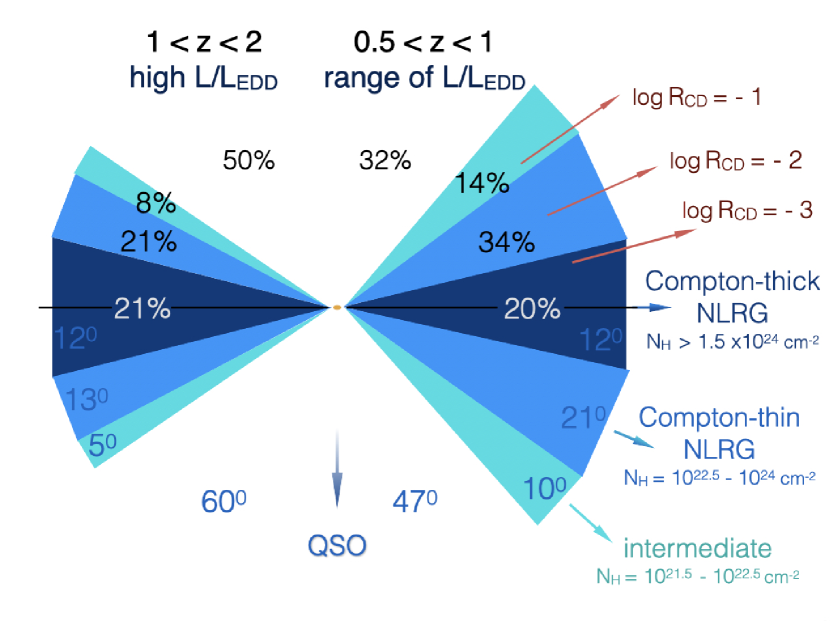
Figure 16: Schematic of geometry of the circumnuclear obscuring dusty region inferred from the number of sources as a function of $N_{\rm H}$ in the high-$z$ sample (Wilkes et al., 2013; represented by the left side of the diagram) and the medium-$z$ 3CRR sample (represented by the right side of the diagram; see also Table 6 for details). Percentages show how many sources are in each category: QSO ($N_{\rm H}$  $<10^{21.5}$ cm^-2), intermediate sources ($N_{\rm H}$$=10^{21.5-22.5}$ cm^-2; light blue), Compton-thin NLRGs ($N_{\rm H}$$=10^{22.5-24}$ cm^-2; blue), and Compton-thick NLRGs ($N_{\rm H}$ $>1.5\times 10^{24}$ cm^-2, dark blue). Red arrows show lines of sight for which the radio core fraction is $\log R_{\rm CD}=-1,-2,-3$. The torus in the high-$z$ sample is more compact due to high $L/L_{\rm Edd}$, while in the medium-$z$ sample the torus is “puffed-up”, which we interpret as due to a larger range of $L/L_{\rm Edd}$ ratios extending to lower values in comparison with the high-$z$ sample (see Section 7.1).

Nine NLRGs are CT candidates characterized by the following Compton-thick indicators: $L$([O iii])/$L$(2–8 keV) $\geq-0.25$, $L$(30 $\mu$m)/$L$(2–8 keV) $>1.8$, $L$(0.5–8 keV)/$L$(178MHz) $<0$, low radio core fraction (log $R_{\rm CD}$ $<-3$), and/or strong 9.7$\mu$m silicate absorption. In the Unification model, these sources are viewed at the highest inclination angles through optically thick material lying in the plane of the torus/accretion disk. The CT candidates represent 20% (9/44) of the total sample which implies that CT material covers an angle of 12°$\pm$3° above and below the equatorial plane of the obscuring structure as shown in Figure 16. The remaining Compton-thin NLRGs (with $10^{22.5}<$ $N_{\rm H}$/cm^-2 $<1.5\times 10^{24}$) cover 21°$\pm$2°. Intermediate column density ($10^{21.5}<$ $N_{\rm H}$/cm^-2 $<10^{22.5}$) sources including five low-$N_{\rm H}$ NLRGs (Section 6.2) and 3C 196, a red broad-line radio galaxy with relatively high $N_{\rm H}$ $=2.7\times 10^{22}$ cm^-2, cover 10°$\pm$4°. Figure 16 shows the geometry of the obscuring material found from these simple estimates, together with the high-$z$ sample (Wilkes et al., 2013), and a summary is given in Table 6. In both samples, the covering factor for CT material is similar (same percentage of CT sources in both samples), but the opening angle of the torus is smaller for the sample at medium-$z$ than at high-$z$ (47° vs. 60°) implying that the Compton-thin ($10^{21.5}-10^{-24}$ cm^-2) part of the obscuring material (torus or accretion disk wind) is more “puffed-up” in the medium-$z$ 3CRR sample.

Fabian et al. (2008) have shown that the long-lived gas and dust clouds in the vicinity of an AGN have a range of column densities that depend on $L/L_{\rm Edd}$ where $N_{\rm H}$/cm^-2 $>5\times 10^{23}\times$ $L/L_{\rm Edd}$. Ricci et al. (2017) studied a sample of local AGN (both Type 1 and 2 with median $z=0.037$) from the all-sky hard-X-ray (14$-$195 keV) Swift Burst Alert Telescope (BAT) survey, for which reliable estimates of BH mass, intrinsic column densities, X-ray luminosities, and $L/L_{\rm Edd}$ were obtained. They found the fraction of CT sources in their hard-X-ray-selected sample to be $\sim$23$\pm$6%, independent of $L/L_{\rm Edd}$, and similar to the fraction in the medium-$z$ and high-$z$ 3CRR samples. However, the fraction of Compton-thin but obscured sources strongly decreases with $L/L_{\rm Edd}$ in their sample from 0.8 for $L/L_{\rm Edd}<0.01$ to 0.2 for $L/L_{\rm Edd}>0.1$. Ricci et al. (2017) therefore suggested a “radiation-regulated Unification” model, where the covering factor of the Compton-thin gas ($10^{22}<$ $N_{\rm H}$/cm^-2 $<10^{24}$) increases with decreasing $L/L_{\rm Edd}$ while the covering factor of the CT gas stays the same. In this model, for lower $L/L_{\rm Edd}$ the obscuring structure (torus/accretion disk wind) is more puffed-up (see their Fig. 4). Our results for the medium-$z$ sample imply the presence of a puffed-up torus in the low-$N_{\rm H}$ NLRGs, suggesting that $L/L_{\rm Edd}$ extends to lower values than those in the high-$z$ sample.

7.2 $N_{\rm H}$ Distribution

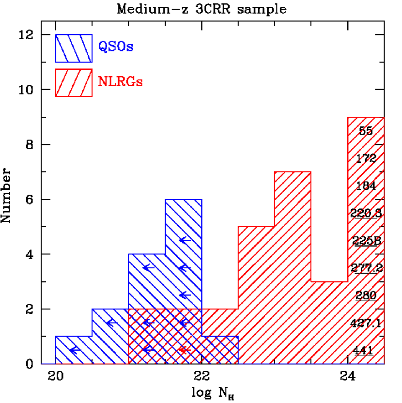
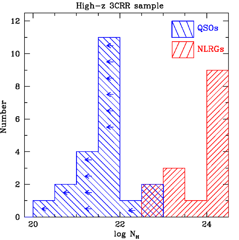
Figure 17: Histograms of the X-ray equivalent intrinsic hydrogen column density $N_{\rm H}$ for the medium-$z$ 3CRR sample (left) and the high-$z$ 3CRR sample (Wilkes et al., 2013) (right). Quasars are shown in blue and NLRGs in red. Upper limits, mostly for quasars with no evidence for intrinsic absorption, are indicated by arrows. Compton-thick NLRGs in the medium-$z$ sample with no measurement of $N_{\rm H}$ due to low $S/N$ are indicated by underlined 3C identification. Note the low $N_{\rm H}$ ($\leq 10^{22}$ cm^-2) NLRGs in the medium-$z$ sample, not present in the high-$z$ sample.

The distributions of the intrinsic $N_{\rm H}$  in the medium-$z$ and the high-$z$ 3CRR samples are presented in Figure 17. The high-$z$ sample (on the right) shows a bimodal distribution, where quasars have $N_{\rm H}$ $<10^{22.5}$ cm^-2, consistent with low obscuration at face-on inclination angles, while the NLRGs show $N_{\rm H}$ $>10^{22.5}$ cm^-2, implying higher obscuration at higher inclination angles, consistent with Unification schemes. There are two quasars with moderate column densities ($10^{22.5}<$ $N_{\rm H}$ /cm^-2 $<10^{23}$) and hard hardness ratios ($0<$ HR $<0.5$) in this sample. In the medium-$z$ sample, the distributions of quasars and NLRGs overlap. Although the quasars show $N_{\rm H}$ $<10^{22.5}$ cm^-2, similar to quasars at high redshifts, the NLRGs have a much broader range of column densities that extend to lower, quasar-like values in the low-$N_{\rm H}$ NLRGs. These NLRGs possibly have low $L/L_{\rm Edd}$, which allows clouds with low column density to form in the vicinity of the central engine (Section 6.3). Such low $L/L_{\rm Edd}$ NLRGs are missing from the high-$z$ sample.

Although a simple Unification model was sufficient to explain the X-ray data and the bimodal $N_{\rm H}$ distribution in the high-$z$ sample, this is not the case in the medium-$z$ sample. An additional parameter, a range of $L/L_{\rm Edd}$, is required to explain the large range of $N_{\rm H}$ in NLRGs seen at intermediate inclination angles, skimming the edge of the torus or accretion disk atmosphere/wind. As a result, the broad range of $L/L_{\rm Edd}$ smears the $N_{\rm H}$ distribution for NLRGs, removing the bimodality that was found in the high-$z$ sample. Turning this argument around, because the Unification model was sufficient for the high-$z$ 3CRR sample, producing a bimodal and narrow $N_{\rm H}$ distribution, the $L/L_{\rm Edd}$ ratio must have a narrower range and higher values compared to the medium-$z$ sample, allowing orientation effects to dominate the properties of the high-$z$ sample. To test this hypothesis, we compiled spectra of the high-$z$ 3CRR quasars (from the SDSS archive, Barthel et al., 1990, M. Vestergaard, D. Stern private communication) and measured the black hole masses from the widths of the C iv and Mg ii emission lines. The masses (measured in 12 out of 20 high-$z$ quasars) are in the range of $M_{\rm BH}=10^{7.7}--10^{9.0}$ M_☉. The radio-to-X-ray SEDs, compiled using data from NED, provided estimates of bolometric luminosities. The inferred $L/L_{\rm Edd}$ ratios are indeed high $>$0.3, implying that orientation dominates the observed properties of the high-$z$ sample, and therefore simple Unification suffices.

7.3 Distribution of intrinsic $L_{\rm X}$

The distribution of intrinsic 0.5–8 keV X-ray luminosity (obtained from HBM modeling; Section 4.5) of the medium-$z$ and the high-$z$ 3CRR populations is presented in Figure 18. The medium-$z$ sample peaks at lower $L_{\rm X}$ (mean log $L_{\rm X}$/erg s${}^{-1}=44.97\pm 0.09$) and has a broader intrinsic $L_{\rm X}$ distribution ($\sigma$=0.51), extending to $\sim$10 times lower $L_{\rm X}$ values than the distribution for the high-$z$ sample (the high-luminosity tail in the medium-$z$ sample is due to a simplistic treatment of piled-up sources for which $N_{\rm H}$ $<10^{21}$ cm^-2 was assumed). The high-$z$ sample shows a narrower distribution ($\sigma$=0.27), peaking at higher $L_{\rm X}$ values (mean log $L_{\rm X}$/erg s${}^{-1}=45.48\pm 0.06$ erg s^-1). Because the intrinsic $L_{\rm X}$ depends on $L/L_{\rm Edd}$ (e.g., Czerny et al., 1996 Fig. 1), we interpret the difference as due to a broad range of $L/L_{\rm Edd}$ in the medium-$z$ sample, extending to lower values, while the high-$z$ sample has higher $L/L_{\rm Edd}$ with a narrower range. The different distributions of intrinsic $N_{\rm H}$ in the two samples is also consistent with this scenario (Section 7.2).

7.4 Obscured fraction

Obscuration in AGN is highly anisotropic and strongly wavelength dependent. Hence the “obscured fraction” defined as the ratio of the number of obscured AGN (either optically classified Type 2s or those with $N_{\rm H}$ $>10^{22}$ cm^-2 in X-ray studies) to all AGN, and its dependence on luminosity and/or redshift differ for samples selected at different wavebands. Optical surveys at low redshift ($z<0.05$) and low (Seyfert) luminosity find obscured fractions of $\sim$0.65–0.75 (Maiolino & Rieke, 1995; Huchra & Burg, 1992; Lawrence & Elvis, 1982), implying there are 2–3 times more Type 2s than Type 1s in the local Universe. High luminosity, radio-selected, and hence unbiased by orientation, samples with $z>0.3$ find an optical obscured fraction of $\sim$0.6, consistent with a torus half-opening angle of $\sim$53° in Unification models (Willott et al., 2000) and a luminosity dependence (Grimes et al., 2005) consistent with the “receding torus model”. X-ray surveys, sensitive to gas rather than dust obscuration and probing deeper into the obscured AGN population, find a wide range of obscured fractions $\sim$0.1–0.8, decreasing with luminosity and increasing with redshift (Hasinger, 2008; Treister & Urry, 2006; La Franca et al., 2005; Sazonov et al., 2012; Burlon et al., 2011), although Ricci et al. (2017), using a local Swift/BAT selected sample, showed that the dependence is primarily with $L/L_{\rm Edd}$.

The obscured fraction in the medium-$z$ 3CRR sample studied in this paper is 0.68 when the optical classification (based on the presence or absence of the broad emission lines in optical spectra) is used. However, if the classification is based on X-rays, where $N_{\rm H}$ $=10^{22}$ cm^-2 is assumed to divide obscured from unobscured sources, then four out of the five low-$N_{\rm H}$ NLRGs will qualify as X-ray unobscured, and 3C 196 a quasar with $N_{\rm H}$ $>10^{22}$ cm^-2 as X-ray obscured, yielding an obscured fraction of 0.61. The ratio of X-ray unobscured ($N_{\rm H}$ $<10^{22}$ cm^-2) to Compton-thin obscured ($10^{22}<$ $N_{\rm H}$ $<1.5\times 10^{24}$) to CT ($N_{\rm H}$ $>1.5\times 10^{24}$) sources is then 1.9:2:1.

In the high-$z$ 3CRR sample the obscured fraction is lower. It is 0.42 if optical classification is used and 0.5 if X-ray classification is used, the difference being due to two quasars with $N_{\rm H}$ $>10^{22}$ cm^-2 classified as obscured in X-rays. The ratio of X-ray unobscured to Compton-thin obscured to CT sources is 2.5:1.4:1.

The difference between optical and X-ray obscured fractions comes from four low-$N_{\rm H}$, low $L/L_{\rm Edd}$ NLRGs in the medium-$z$ 3CRR sample and two high-$N_{\rm H}$, high $L/L_{\rm Edd}$ quasars in the high-$z$ sample. In the former case the X-ray obscured fraction is lower in comparison with the optical obscured fraction, while in the latter case (high $L/L_{\rm Edd}$ sample) it is higher.

As shown above, the obscured fraction is an inaccurate tool for measuring the level of obscuration in a sample. Not only does the obscured fraction depend on the sample’s wavelength selection, luminosity, and redshift but also on whether optical or X-ray classification is used. It also depends on the sample’s $L/L_{\rm Edd}$ range, which defines the geometry of the obscuring material (more puffed-up torus for lower $L/L_{\rm Edd}$, see Section 7.1) and number of sources with inconsistent optical and X-ray type.

7.5 Sources with inconsistent optical and X-ray types

The obscured AGN fraction in the medium-$z$ and high-$z$ samples differs slightly depending on whether the source classification is based on optical spectra or X-ray data. Merloni et al. (2014) studied AGN with a wide range of redshifts ($0.3<z<3.5$) in the XMM-COSMOS survey and found that setting the dividing line between Type 1 and Type 2 at $N_{\rm H}$ $=10^{21.5}$ cm^-2 rather than 10²² cm^-2 gives a better correspondence between optical and X-ray type. However, even then $\sim$30% of AGN in their sample have conflicting optical and X-ray classifications. At dust extinctions $A_{\rm V}=5$–6 mag, the broad emission lines H$\beta$ and H$\alpha$ are totally obscured. This corresponds to column densities $N_{\rm H}$ $=(0.9--1.1)\times 10^{22}$ cm^-2 for a Galactic dust-to-gas ratio. A small (factor of a few) divergence from the Galactic dust-to-gas ratio will result in inconsistent X-ray and optical classifications around the dividing Type1/Type2 column density of $N_{\rm H}$ $=10^{22}$ cm^-2.

Merloni et al. (2014) found that the AGN with conflicting optical and X-ray type can be divided into two classes:

• optical Type 1 and X-ray Type 2 sources, which are high-luminosity broad-line AGN with X-rays absorbed by dust-free material lying at sub-parsec scales, and

• optical Type 2 and X-ray Type 1 sources, which are low-luminosity, unobscured AGN where the broad lines are probably diluted by the host galaxy.

The radio-selected 3CRR sample can give further insight into the nature of sources with inconsistent optical and X-ray classifications:

1. The high-$z$ sample has 2 quasars (optical Type 1) with high column density of $N_{\rm H}$=10^22.7-23 cm^-2 and HR $>0$ (X-ray Type 2). These sources (3C 68.1, 325) have high $L/L_{\rm Edd}>0.3$ , intermediate viewing angles ($-3<$ log $R_{\rm CD}$ $<-2$), where our line of sight is skimming the edge of the accretion disk or torus. In these high $L/L_{\rm Edd}$ sources, the X-rays are possibly obscured by gas in the strong, outflowing accretion disk wind (Luo et al., 2015; Ni et al., 2018), while the BLR is visible directly. Because of strong UV radiation pressure (high $L/L_{\rm Edd}$), the low-$N_{\rm H}$ gas and dust clouds are blown away.

2. The medium-$z$ 3CRR sample has 5 NLRGs (optical Type 2) with low column density $N_{\rm H}$ $<10^{22}$ cm^-2 and quasar-like HR $<0$ (X-ray Type 1). They have intermediate viewing angles, skimming the edge of the torus/accretion disk. These NLRGs have low $L/L_{\rm Edd}$, which allows low-$N_{\rm H}$ clouds to survive in the vicinity of the nucleus and results in a “puffed-up” torus (see Section 6.3), which can hide the broad-line region.

In both the high- and medium-$z$ 3CRR samples, AGN with conflicting optical/X-ray types have intermediate radio core fractions ($-3<$ log $R_{\rm CD}$ $<-2$), where viewing angles are skimming the edge of the accretion disk or torus. In this regime, the torus and accretion disk are most vulnerable to changes in the $L/L_{\rm Edd}$ ratio. We find that sources classified as optical Type 1 and X-ray Type 2 (X-ray obscured quasars) have high $L/L_{\rm Edd}$ ratio, where the strong accretion disk winds obscure the X-rays. The optical Type 2 and X-ray Type 1 sources (unobscured NLRGs) are low $L/L_{\rm Edd}$ AGN, where the edge or atmosphere of the “puffed-up” dusty torus provides obscuration for both the X-rays and the BLR.

8 Summary

A complete, flux-limited (10 Jy), low-frequency (178 MHz) radio-selected, and so unbiased by the effects of orientation and obscuration sample of $0.5<z<1$ 3CRR sources has now been observed with Chandra. The sample includes 14 quasars (no blazars), 29 NLRGs, and 1 LERG with similar (within $\sim$1.5 dex) 178 MHz extended radio luminosities (i.e., similar intrinsic AGN luminosities). All sources are radio luminous and of FR II type, meaning they all harbor a powerful AGN in their nucleus. The radio core fraction $R_{\rm CD}$ provides an estimate of the viewing angle (with respect to the radio jet) and so nuclear orientation. We study the dependence of X-ray, mid-IR, and radio properties on orientation and obscuration and other central engine parameters ($L/L_{\rm Edd}$), and compare our results with the high-$z$ ($1<z<2$) 3CRR sample (Wilkes et al., 2013) allowing investigation of redshift and luminosity-dependent effects on obscuration relative to orientation. We find:

1. Modified AGN Unification. Quasars in the medium-$z$ ($0.5<z<1$ ) 3CRR sample have high observed X-ray luminosities $L_{\rm X}$(0.5$-$8 keV) $\sim 10^{44.8}$–$10^{45.9}$ erg s^-1, soft hardness ratios (HR $<0$), and high radio core fractions (log $R_{\rm CD}$ $>-2$), implying low obscuration ($N_{\rm H}$ $<10^{22.5}$ cm^-2) and face-on orientation. By contrast, NLRGs have 10–1000 times lower observed (uncorrected for obscuration) X-ray luminosities $L_{\rm X}$(0.5$-$8 keV) $\sim 10^{42.9}$–$10^{45.1}$ erg s^-1 despite having similar radio luminosities to quasars, a wide range of hardness ratios ($-0.6<HR<0.9$) and low radio core fractions (log $R_{\rm CD}$ $<-1.9$). This combination of properties implies a range of obscuration ($N_{\rm H}$ $>10^{21}$ cm^-2) and edge-on orientation. These properties together with the observed trend of increasing X-ray obscuration (expressed by $N_{\rm H}$ and decreasing $L_{\rm X}$/$L$(178 MHz) with decreasing radio core fraction $R_{\rm CD}$ (Figure 10), are consistent with the orientation-dependent obscuration of Unification models. However, an additional variable, a range of $L/L_{\rm Edd}$, is needed to explain the large range of column densities ($N_{\rm H}$ $=10^{21.5}$–$10^{23.5}$ cm^-2) found in NLRGs observed at intermediate viewing angles ($-3<$ log $R_{\rm CD}$ $<-2$) and the sample’s broad and smooth distributions of intrinsic column densities and intrinsic X-ray luminosities.

2. $L/L_{\rm Edd}$ dependence on redshift. In the high-$z$ 3CRR sample (Wilkes et al., 2013), a simple Unification model was sufficient to explain the multiwavelength properties of the sample, suggesting a narrower range of $L/L_{\rm Edd}$ and orientation effects dominating the observed properties. We estimate that $L/L_{\rm Edd}$ is high $>$0.3, possibly due to higher gas supply in the denser galaxy environments at higher redshifts. The narrow range and higher values of $L/L_{\rm Edd}$ produce a bimodal distribution of $N_{\rm H}$ and a narrower distribution of intrinsic X-ray luminosities, peaking at higher $L_{\rm X}$, in comparison with the medium-$z$ sample.

3. Low-$N_{\rm H}$ NLRGs. Five NLRGs (3C 6.1, 175.1, 228, 263.1, 445) in the medium-$z$ sample show unusually low intrinsic column densities ($21<$ log $N_{\rm H}$/cm^-2 $<22.1$). They have high, quasar-like $L_{\rm X}$ and $L_{\rm X}/L_{\rm R}$ ratios, soft HR, low mid-IR emission, and intermediate viewing angles. Analysis of their properties suggest a low $L/L_{\rm Edd}$ resulting in a puffed-up dusty torus.

4. Covering factor. The medium-$z$ and high-$z$ samples have similar fractions of Compton-thick sources ($\sim$20%), but there are relatively fewer quasars (32% vs. 50%) and more Compton-thin NLRGs in the medium-$z$ sample (45% vs. 29%), implying a larger covering factor of the Compton-thin material or a “puffed-up” torus. We interpret this as being due to $L/L_{\rm Edd}$ extending to lower values ($\sim$0.01) in the medium-$z$ 3CRR sample, allowing lower column density material to remain in the “atmosphere” of the torus.

5. Geometry of the obscuring material. Assuming a random distribution of source orientation on the sky and a simple geometry in which the obscuring material lies in a disk or torus perpendicular to the radio jet, we conclude that Compton-thick obscuring material extends $\sim$12° above and below the disk/torus midplane, additional Compton-thin obscuring material extends for another $\sim$31° with the density diminishing with viewing angle, and the remaining $\sim$47°(torus opening angle) are unobscured. In the high-$z$ sample Compton thick material occupied 12° below and above the midplane, Compton-thin material 18°, and the torus opening angle was 60°.

6. Compton-thick sources. Nine NLRGs (3C 55, 172, 184, 220.3, 225B, 277.2, 280, 427.1, 441) are likely Compton-thick based on several Compton-thick indicators: $L$[O iii]/$L$(2–8 keV) $\geq-0.25$, $L$(30 $\mu$m)/$L$(2–8 keV) $>1.8$, low radio core fraction (log $R_{\rm CD}$ $\leq-3$) and/or strong 9.7$\mu$m silicate absorption. Comparison of different Compton-thick indicators shows that $L$([O iii])/$L$(2–8 keV) $\geq-0.25$ is most robust, available for both the radio-quiet and radio-loud AGN, and independent of $L/L_{\rm Edd}$. The $L$(30 $\mu$m)/$L$(2–8 keV) ratio is dependent on $L/L_{\rm Edd}$, and only Compton-thick sources with high, quasar-like $L/L_{\rm Edd}$ ratios have values $>$1.8. The strength of the silicate absorption is affected by dust lying at host galaxy scales and dust related to mergers.

7. Obscured fractions. The ratio of the unobscured ($N_{\rm H}$ $\leq 10^{22}$ cm^-2) to Compton-thin obscured to Compton-thick ($N_{\rm H}$ $\geq 1.5\times 10^{24}$ cm^-2) sources in the medium-$z$ sample is 1.9:2:1, and the obscured fraction is $=0.61$. In comparison, this ratio in the high-$z$ sample is 2.5:1.4:1, and the obscured fraction is 0.5, implying a larger torus opening angle (60°$\pm$8° vs. 47°$\pm$3°). If the sources in the medium-$z$ sample are divided according to optical spectral type, a slightly different ratio is found: quasars to Compton-thin NLRGs to Compton-thick NLRGs = 1.6:2.3:1, and the obscured fraction is 0.68. The difference between the optical and X-ray derived obscured fractions is due to a few intermediate $N_{\rm H}$ sources with inconsistent optical and X-ray Type1/Type2 classifications.

8. Inconsistent optical and X-ray type sources. Four low-$N_{\rm H}$ NLRGs from the medium-$z$ sample and two high-$N_{\rm H}$ quasars from the high-$z$ sample (3C 68.1, 325) have inconsistent optical and X-ray Type1/Type2 classifications. These sources have intermediate inclination angles (i.e., lines of sight skimming the edge of the torus or accretion disk) and have $N_{\rm H}$ $\sim$ 10²² cm^-2. For high $L/L_{\rm Edd}>0.3$, we observe an optical Type 1, X-ray Type 2 source (obscured quasar), where the X-ray obscuration is due to a strong accretion disk wind, and for low $L/L_{\rm Edd}\sim 0.01$ an optical Type 2, X-ray Type 1 source (unobscured NLRG), where a puffed-up dusty torus provides obscuration and hides the broad-line region.

Table 1: X-ray Observations and Radio Data for the Medium Redshift 3CRR Sample

Name	redshift	Source	Chandra	Date Obs.	Exp. time	X-ray	RA	Dec.	Pos.	Galactic	Fν(5GHz)	Ref.	Fν(5GHz)	Ref.	log Lν(5GHz)	log $R_{\rm CD}$	log L([OIII]) b
		Type	OBSID	UT	ks	Ref.	J2000.0	J2000	Ref.	NH a	Core		Total		Total		[W]
										$10^{20}$ cm-2	[mJy]		[Jy]		[erg s-1 Hz-1]
3C 6.1	0.840	G	3009	2002 Oct 15	36.49	3,4,7,11,12	00:16:31.1	+79:16:50	M06	14.80	4.4	H94	1.087	H94	34.58	-2.39	35.37f
3C 6.1	0.840	G	4363	2002 Aug 26	19.90	3,4,7,11,12	00:16:31.1	+79:16:50	M06	14.80	4.4	H94	1.087	H94	34.58	-2.39	35.37f
3C 22	0.936	G	14994	2013 Jun 05	9.35		00:50:56.2	+51:12:03	M06	17.20	7.3	F97	0.76	F93	34.54	-2.01	36.44f
3C 34	0.689	G	16046	2014 Sep 25	11.92	15	01:10:18.5	+31:47:19	M06	5.62	1.03	J95	0.381	J95	33.91	-2.57	36.44f
3C 41	0.795	G	16047	2014 Sep 03	11.89	15	01:26:44.3	+33:13:11	M06	5.05	0.64	W99	1.45	L80	34.65	-3.35	35.66f
3C 49	0.621	G/CSS	14995	2013 Aug 31	9.45		01:41:09.1	+13:53:28	D96	4.79	7.7	L98	0.894	H94	34.17	-2.06	35.79
3C 55	0.735	G/CT	16050	2014 Jun 15	11.92	15	01:57:10.5	+28:51:39	M06	5.48	3.4	F93	0.88	F93	34.35	-2.40	35.35f
3C 138	0.759	Q/CSS	14996	2013 Mar 22	2.00		05:21:09.8	+16:38:22	Z14	23.80	485	F89	3.34	F89	34.96	-0.77	36.46
3C 147	0.545	Q/CSS	14997	2013 Aug 26	2.00		05:42:36.1	+49:51:07	M98	20.50	2500	L98	7.456	L98	34.96	-0.30	36.79
3C 172	0.519	G/CT	14998	2013 Sep 05	9.95		07:02:08.3	+25:13:53	G04	7.98	0.5c	G04	0.844	L80	34.59	-3.23	36.08f
3C 175	0.770	Q	14999	2013 Feb 21	2.00		07:13:02.4	+11:46:16	M06	10.50	23.5	B94	0.687	G91	34.29	-1.45	36.10
3C 175.1	0.920	G	15000	2013 Feb 10	9.94		07:14:04.6	+14:36:22	M06	8.99	1.1	M06	0.556	L80	34.39	-2.70	35.96f
3C 184	0.994	G/CT	3226	2002 Sep 22	18.89	3	07:39:24.4	+70:23:10	D96	3.45	$<$0.2	M06	0.596	L80	34.50	$<$-3.47	36.22f
3C 184 d	0.994	G/CT	0028540601	2002 Mar 10	40.9	3	07:39:24.4	+70:23:10	D96	3.45	$<$0.2	M06	0.596	L80	34.50	$<$-3.47	36.22f
3C 184 d	0.994	G/CT	0028540201	2001 Sep 19	38.9	3	07:39:24.4	+70:23:10	D96	3.45	$<$0.2	M06	0.596	L80	34.50	$<$-3.47	36.22f
3C 196	0.871	Q	15001	2013 Mar 23	2.00		08:13:36.0	+48:13:02	M06	4.55	11.6	M06	4.329	L80	35.22	-2.57	36.08
3C 207	0.681	Q	2130	2000 Nov 04	37.54	1,3,6,9,16,17,19	08:40:47.5	+13:12:23	M06	4.12	539	M06	1.43	L80	34.47	-0.22	36.05
3C 216	0.670	Q/CSS	15002	2013 Feb 25	2.00		09:09:33.5	+42:53:46	M06	1.60	1050	H89	1.797	H89	34.57	0.15	$<$35.46
3C 220.3	0.685	G/CT	14992	2013 Jan 21	9.94		09:39:23.8	+83:15:25	H14	3.65	$<$0.2	M06	0.636	L80	34.12	$<$-3.50	36.00f
3C 225B	0.580	G/CT	16058	2014 Oct 18	11.92	15	09:42:15.4	+13:45:50	M18	3.50	1.11	G04	0.97	G04	34.14	-2.94	35.58f
3C 226	0.818	G	15003	2013 Oct 07	9.94		09:44:16.5	+09:46:16	M06	2.97	4.4c	M06	0.636	L80	34.14	-2.16	36.04f
3C 228	0.552	G	2095	2001 Jun 03	13.78	3,12	09:50:10.7	+14:20:00	G04	3.18	13.3	G88	1.132	L80	34.35	-1.92	35.36f
3C 228	0.552	G	2453	2001 Apr 23	10.61	3,12	09:50:10.7	+14:20:00	G04	3.18	13.3	G88	1.132	L80	34.35	-1.92	35.36f
3C 247	0.749	G	16060	2014 Sep 26	11.64	15	10:58:59.0	+43:01:24	M97	1.06	3.5	G88	0.95	F14	34.40	-2.43	35.92f
3C 254	0.737	Q	2209	2001 Mar 26	29.67	8,5,3,13,18	11:14:38.7	+40:37:20	W12	1.90	19	H89	0.747	L80	34.21	-1.58	36.71
3C 263	0.646	Q	2126	2000 Oct 28	49.19	3,5,7,10,13,18	11:39:57.0	+65:47:49	M06	1.18	161	M06	1.033	L80	34.32	-0.73	36.71
3C 263.1	0.824	G	15004	2013 Mar 20	9.94		11:43:25.0	+22:06:56	M06	2.12	1.4	M06	0.775	H94	34.23	-2.74	36.31f
3C 265	0.811	G	2984	2002 Apr 25	58.92	2,3	11:45:28.9	+31:33:46	M06	1.90	2.65	F93	0.63	F93	34.13	-2.37	36.80
3C 268.1	0.970	G	15005	2013 Jul 08	9.94		12:00:24.4	+73:00:45	M06	1.97	2.0	G88	2.602	L80	34.78	-3.11	35.51f
3C 275.1	0.557	Q	2096	2001 Jun 02	24.76	15	12:43:57.7	+16:22:53	G04	1.98	207	G04	0.910	F14	34.07	-0.53	35.62f
3C 277.2	0.766	G/CT	16063	2015 May 07	11.91	15	12:53:33.3	+15:42:31	M06	1.96	0.48	W99	0.576	L80	34.21	-3.08	36.10f
3C 280	0.996	G/CT	2210	2001 Aug 27	63.52	3,8,11,13,14	12:56:57.8	+47:20:19	Xraye	1.13	$<$0.7	M06	1.519	L80	34.55	$<$-3.34	37.14f
3C 286	0.850	Q/CSS	15006	2013 Feb 26	2.00		13:31:08.2	+30:30:32	M98	1.15	…	…	7.584	A95	35.49	…	35.99f
3C 289	0.967	G	15007	2013 Jul 28	9.70		13:45:26.2	+49:46:32	M06	1.15	0.8	M06	0.596	L80	34.38	-2.87	35.46f
3C 292	0.710	G	17488	2014 Nov 21	7.97	15	13:50:41.8	+64:29:35	B06	2.12	1	W99	0.702	B91	34.22	-2.85	36.33g
3C 309.1	0.905	Q/CSS	3105	2002 Jan 28	16.95	3	14:59:07.5	+71:40:19	M98	2.30	804	LM97	3.734	L80	35.16	-0.56	36.70
3C 330	0.550	G	2127	2001 Oct 16	44.18	3	16:09:34.9	+65:56:37	G04	2.81	0.74	F97	2.35	F93	34.90	-3.50	36.57f
3C 334	0.555	Q	2097	2001 Aug 22	32.47	3	16:20:21.8	+17:36:23	G04	4.24	111	B94	0.566	L80	34.28	-0.61	36.37
3C 336	0.927	Q	15008	2013 Mar 03	2.00		16:24:39.0	+23:45:12	M06	4.47	21.3	M06	0.685	L80	34.43	-1.49	36.46
3C 337	0.635	G	15009	2013 Oct 05	9.95		16:28:52.5	+44:19:06	M06	1.05	0.3	M06	0.904	L80	34.50	-3.48	34.76f
3C 340	0.775	G	15010	2013 Oct 20	9.95		16:29:36.5	+23:20:12	M06	4.04	1.2	M06	0.685	L80	34.40	-2.76	35.96f
3C 343	0.988	G/CSS	15011	2013 Apr 28	9.94		16:34:33.7	+62:45:35	K81	2.67	$<$300	P81	1.48	L80	34.78	$<$-0.59	35.68
3C 343.1	0.750	G/CSS	15012	2013 Feb 25	9.94		16:38:28.1	+62:34:44	P11	2.70	$<$200	G88	1.192	L80	34.64	$<$-0.70	35.71
3C 352	0.807	G	15013	2013 Oct 10	9.95		17:10:44.1	+46:01:28	M06	2.41	3.4	M06	0.467	L80	34.24	-2.13	36.66f
3C 380	0.692	Q/CSS	3124	2002 May 20	5.33	3	18:29:31.7	+48:44:46	P06	5.67	4500	LM97	7.447	L80	35.42	0.18	36.76
3C 427.1	0.572	LINER/CT	2194	2002 Jan 27	39.45	3	21:04:06.9	+76:33:10	G04	10.90	1.0c	G04	0.953	L80	34.51	-2.98	36.07g
3C 441	0.708	G/CT	15656	2013 Jun 26	6.98		22:06:04.9	+29:29:19	D96	8.32	3.5	F97	1.005	H94	34.56	-2.46	35.68f
3C 455	0.543	G/CSS	15014	2013 Aug 13	9.95		22:55:03.8	+13:13:34	B94	4.99	1.6c	B94	0.923	L80	34.49	-2.76	36.07

^a Galactic equivalent hydrogen column density from Dickey & Lockman (1990). ^b The [O iii]$\lambda 5007$ luminosity from (Grimes et al., 2004). ^c The 5 GHz data are unavailable, so an 8 GHz flux was used to calculate the 5 GHz flux assuming a radio spectral index of $\alpha=0.7$ for the radio-lobes and $\alpha=0.3$ for the radio-core ($F_{\nu}\propto\nu^{-\alpha}$). ${}^{d}~{}$XMM data. ^e No radio core position available - position from Chandra image. ^f L([O iii]) determined from [O ii]$\lambda$3727 emission using the L([O ii]) vs. L([O iii]) relation from Grimes et al. (2004). ^g L([O iii]) determined from radio luminosity L(151MHz) (Grimes et al., 2004).
X-ray references: 1: Brunetti et al. (2002), 2: Bondi et al. (2004), 3: Belsole et al. (2006), 4: Belsole et al. (2007), 5: Crawford & Fabian (2003), 6: Cheung (2004), 7: Croston et al. (2005), 8: Donahue et al. (2003), 9: Gambill et al. (2003), 10: Hardcastle et al. (2002), 11: Hardcastle et al. (2004), 12: Hardcastle et al. (2009), 13: Haggard et al. (2010), 14: Massaro et al. (2011), 15: Massaro et al. (2018), 16: Sambruna et al. (2004), 17: Schwartz et al. (2004), 18: Shang et al. (2011), 19: Tavecchio et al. (2005), Radio references: A95 - Akujor & Garrington (1995), B94 - Bridle et al. (1994), B06 - Belsole et al. (2006), F89 - Fanti et al. (1989), F93 - Fernini et al. (1993), F97 - Fernini et al. (1997), G88 - Giovannini et al. (1988), G91 - Gregory & Condon (1991), G04 - Gilbert et al. (2004), H89 - Hough & Readhead (1989), H94 - Hutchings et al. (1994), L80 - Laing & Peacock (1980), L98 - Ludke et al. (1998), LM97 - Laurent-Muehleisen et al. (1997), M97 - McCarthy et al. (1997), M06 - Mullin et al. (2006), P81 - Pearson & Readhead (1981), P88 - Pearson & Readhead (1988). Positions from radio data: B94 - Bogers et al. (1994), D96 - Douglas et al. (1996), H14 - Haas et al. (2014), K81 - Kuehr et al. (1981), M98 - Ma et al. (1998), P06 - Petrov et al. (2006), P11 - Petrov & Taylor (2011), W99 - Willott et al. (1999), Positions from optical and radio: Z14 - Zacharias & Zacharias (2014), Optical position from SDSS: W12 - Wu et al. (2012)

Table 2: X-ray Source Parameters

Name	Chandra	Net Cts	Bkgrd. Cts	F(0.5$-$8 keV)	log L(0.5$-$8 keV)	$\Gamma$	$N_{\rm H}$	f(1 keV)	Reduced	F(0.5$-$8 keV)	F(0.5$-$8 keV)	log L(0.5$-$8 keV)	HR
	OBSID	(0.5-8 keV)	(0.5-8 keV)	Srcflux	Srcflux		$10^{22}$cm-2	$10^{-6}$	$\chi^{2}$	Observed	Intrinsic
(1)	(2)	(3)	(4)	(5)	(6)	(7)	(8)	(9)	(10)	(11)	(12)	(13)	(14)
3C 6.1	3009	$1718.8\pm 41.5$	$1.22\pm 0.08$	$33.60^{+0.80}_{-0.90}$	$45.04^{+0.01}_{-0.01}$	1.76${}^{+0.10}_{-0.09}$	$0.32^{+0.13}_{-0.12}$	$14.52^{+1.44}_{-1.28}$	0.7	$43.59^{+5.03}_{-5.05}$	$47.33^{+7.20}_{-5.81}$	$45.19^{+0.06}_{-0.06}$	$-0.29^{+0.02}_{-0.02}$
3C 6.1	4363	$811.1\pm 28.5$	$0.87\pm 0.07$	$28.90^{+1.10}_{-1.00}$	$44.98^{+0.02}_{-0.02}$	1.62${}^{+0.12}_{-0.12}$	$0.26^{+0.14}_{-0.12}$	$11.26^{+1.39}_{-1.23}$	0.7	$39.97^{+7.38}_{-5.55}$	$42.91^{+8.76}_{-7.35}$	$45.15^{+0.08}_{-0.08}$	$-0.29^{+0.03}_{-0.03}$
3C 22	14994	$68.8\pm 8.3$	$0.22\pm 0.03$	$4.38^{+0.72}_{-0.65}$	$44.27^{+0.07}_{-0.07}$	1.9	$21.24^{+16.02}_{-7.36}$	$11.31^{+6.21}_{-3.64}$	0.5	$12.53^{+5.62}_{-5.03}$	$31.14^{+15.71}_{-10.35}$	$45.13^{+0.18}_{-0.18}$	$0.59^{+0.11}_{-0.08}$
3C 34	16046	$73.7\pm 8.6$	$0.32\pm 0.04$	$6.18^{+0.79}_{-0.79}$	$44.12^{+0.06}_{-0.05}$	1.9	$12.32^{+3.09}_{-3.09}$	$56.31^{+13.44}_{-13.44}$	0.21	$5.70^{+1.52}_{-1.52}$	$25.37^{+0.33}_{-0.33}$	$44.74^{+0.01}_{-0.01}$	$0.67_{-0.08}^{+0.09}$
3C 41	16047	$37.5\pm 6.1$	$0.47\pm 0.05$	$2.40^{+0.46}_{-0.52}$	$43.87^{+0.09}_{-0.09}$	1.9	$29.45^{+13.11}_{-13.11}$	$48.37^{+21.75}_{-21.75}$	0.21	$2.86^{+1.42}_{-1.42}$	$16.81^{+0.30}_{-0.30}$	$44.71^{+0.01}_{-0.01}$	$0.78_{-0.08}^{+0.12}$
3C 49	14995	$161.8\pm 12.7$	$0.24\pm 0.03$	$12.30^{+1.00}_{-1.00}$	$44.29^{+0.03}_{-0.04}$	1.9	$6.38^{+1.11}_{-0.91}$	$17.64^{+2.63}_{-2.49}$	0.2	$25.16^{+3.46}_{-3.22}$	$52.81^{+6.33}_{-8.09}$	$44.92^{+0.05}_{-0.07}$	$0.39^{+0.09}_{-0.06}$
3C 55	16050	$15.6\pm 4.0$	$0.35\pm 0.04$	$17.70^{+4.20}_{-4.90}$	$44.65^{+0.12}_{-0.11}$	1.9	…	$2.27^{+0.98}_{-0.98}$	0.4	$1.08^{+0.40}_{-0.40}$	…	…	$-0.12_{-0.27}^{+0.22}$
3C 138	14996	$388.9\pm 19.7$	$0.10\pm 0.02$	$193.00\pm 10.00$	$45.70^{+0.02}_{-0.02}$	1.9	$<0.96$	$71.07^{+7.51}_{-6.74}$	1.2	$192.48^{+24.94}_{-29.60}$	$211.64^{+17.16}_{-18.91}$	$45.74^{+0.03}_{-0.04}$	$-0.15^{+0.05}_{-0.05}$
3C 147	14997	$151.0\pm 12.3$	$0.04\pm 0.01$	$81.30^{+6.70}_{-6.60}$	$44.98^{+0.03}_{-0.04}$	1.9	$<0.95$	$30.61^{+4.48}_{-4.21}$	0.3	$79.41^{+12.55}_{-10.78}$	$91.97^{+11.84}_{-17.82}$	$45.03^{+0.05}_{-0.09}$	$-0.31^{+0.07}_{-0.08}$
3C 172	14998	$31.7\pm 5.7$	$0.30\pm 0.05$	$1.84^{+0.44}_{-0.37}$	$43.28^{+0.09}_{-0.10}$	1.9	$82.97^{+75.16}_{-42.29}$	$31.92^{+82.59}_{-21.31}$	0.5	$6.88^{+13.59}_{-5.21}$	$135.73^{+70.93}_{-87.35}$	$45.15^{+0.18}_{-0.45}$	$0.73^{+0.13}_{-0.10}$
3C 175	14999	$354.9\pm 18.8$	$0.07\pm 0.03$	$155.00^{+8.00}_{-9.00}$	$45.62^{+0.02}_{-0.03}$	1.9	$<0.56$	$54.81^{+5.41}_{-5.01}$	0.7	$152.51^{+13.15}_{-17.48}$	$162.99^{+14.80}_{-16.42}$	$45.64^{+0.04}_{-0.05}$	$-0.32^{+0.05}_{-0.05}$
3C 175.1	15000	$88.7\pm 9.4$	$0.31\pm 0.04$	$6.72^{+0.76}_{-0.75}$	$44.44^{+0.05}_{-0.05}$	1.9	$1.23^{+0.79}_{-0.56}$	$3.73^{+0.80}_{-0.72}$	0.2	$8.62^{+2.00}_{-1.77}$	$11.40^{+2.00}_{-2.03}$	$44.67^{+0.07}_{-0.08}$	$-0.21^{+0.10}_{-0.10}$
3C 184	3226	$47.5\pm 6.9$	$0.47\pm 0.05$	$1.17^{+0.20}_{-0.17}$	$43.76^{+0.07}_{-0.07}$	1.9	$<2.23$	$0.24^{+0.13}_{-0.09}$	0.3	$2.07^{+0.21}_{-0.27}$	$0.72^{+0.35}_{-0.34}$	$43.55^{+0.17}_{-0.28}$	$0.30^{+0.15}_{-0.12}$
3C 184 a	XMM	$776\pm 65$	…	$1.75^{+0.27}_{-0.24}$	$43.94^{+0.06}_{-0.06}$	$1.4^{+0.3}_{-0.2}$	$48.7^{+22.0}_{-12.1}$	$24^{+11}_{-10}$	39.3	$17^{+7}_{-6}$	…	$44.8^{+0.1}_{-0.2}$	…
3C 196	15001	$89.9\pm 9.5$	$0.07\pm 0.02$	$32.60^{+3.60}_{-3.60}$	$45.07^{+0.05}_{-0.05}$	1.9	$2.68^{+1.17}_{-0.85}$	$24.85^{+5.60}_{-5.06}$	0.1	$48.60^{+11.40}_{-11.55}$	$70.97^{+14.98}_{-13.87}$	$45.41^{+0.08}_{-0.09}$	$-0.07^{+0.10}_{-0.10}$
3C 207	2130	$6462.7\pm 80.4$	$8.34\pm 0.21$	$85.40^{+1.10}_{-1.10}$	$45.23^{+0.01}_{-0.01}$	2.15${}^{+0.07}_{-0.06}$	$0.29^{+0.05}_{-0.04}$	$66.05^{+3.76}_{-3.53}$	0.9	$141.60^{+12.41}_{-8.78}$	$165.25^{+13.72}_{-12.74}$	$45.52^{+0.03}_{-0.03}$	$-0.29^{+0.01}_{-0.01}$
3C 216	15002	$247.9\pm 15.7$	$0.07\pm 0.02$	$89.90\pm 5.80$	$45.23^{+0.03}_{-0.03}$	1.9	$0.43^{+0.18}_{-0.15}$	$39.73^{+4.53}_{-4.29}$	0.6	$102.39^{+9.91}_{-14.21}$	$119.58^{+11.94}_{-15.37}$	$45.36^{+0.04}_{-0.06}$	$-0.34^{+0.05}_{-0.06}$
3C 220.3	14992	$5.7\pm 2.4$	$0.28\pm 0.04$	$0.46^{+0.22}_{-0.17}$	$42.97^{+0.17}_{-0.20}$	1.9	…	$<0.45$	0.1	…	…	…	$-0.33^{+0.29}_{-0.46}$
3C 225B	16058	$12.6\pm 3.6$	$0.40\pm 0.04$	$0.84^{+0.23}_{-0.27}$	$43.07^{+0.14}_{-0.12}$	1.9	…	$2.04^{+0.93}_{-0.93}$	0.2	$0.98^{+0.35}_{-0.35}$	…	…	$-0.23_{-0.30}^{+0.23}$
3C 226	15003	$58.8\pm 7.7$	$0.21\pm 0.04$	$3.67^{+0.57}_{-0.51}$	$44.05^{+0.06}_{-0.06}$	1.9	$16.23^{+7.57}_{-4.78}$	$7.90^{+2.89}_{-2.42}$	0.5	$8.99^{+3.30}_{-3.38}$	$22.40^{+9.14}_{-6.90}$	$44.84^{+0.15}_{-0.16}$	$0.56^{+0.13}_{-0.08}$
3C 228	2095	$341.6\pm 18.5$	$0.45\pm 0.07$	$14.20^{+0.80}_{-0.70}$	$44.23^{+0.02}_{-0.02}$	1.9	$0.11^{+0.07}_{-0.06}$	$5.49^{+0.53}_{-0.51}$	0.5	$15.41^{+1.87}_{-1.57}$	$16.65^{+1.26}_{-1.76}$	$44.30^{+0.03}_{-0.05}$	$-0.57^{+0.04}_{-0.04}$
3C 228	2453	$251.6\pm 15.9$	$0.43\pm 0.07$	$13.20^{+0.80}_{-0.80}$	$44.20^{+0.03}_{-0.03}$	1.9	$<0.24$	$4.56^{+0.53}_{-0.39}$	0.6	$13.40^{+1.70}_{-1.82}$	$13.66^{+1.06}_{-1.86}$	$44.21^{+0.03}_{-0.06}$	$-0.58^{+0.05}_{-0.05}$
3C 247	16060	$42.7\pm 6.6$	$0.33\pm 0.04$	$2.78^{+0.44}_{-0.51}$	$43.87^{+0.07}_{-0.07}$	1.9	$7.56^{+2.87}_{-2.87}$	$23.53^{+7.42}_{-7.42}$	0.4	$3.99^{+0.95}_{-0.95}$	$10.48^{+0.37}_{-0.37}$	$44.44^{+0.02}_{-0.02}$	$0.43_{-0.13}^{+0.15}$
3C 254	2209	$5087.4\pm 71.3$	$1.64\pm 0.11$	$88.60^{+1.20}_{-1.20}$	$45.33^{+0.01}_{-0.01}$	1.99${}^{+0.06}_{-0.06}$	$0.08^{+0.04}_{-0.04}$	$47.56^{+2.60}_{-2.48}$	0.6	$128.68^{+7.87}_{-10.20}$	$132.12^{+6.28}_{-6.77}$	$45.50^{+0.02}_{-0.02}$	$-0.43^{+0.01}_{-0.01}$
3C 263	2126	$9061.1\pm 95.2$	$2.89\pm 0.18$	$88.60^{+0.90}_{-0.90}$	$45.19^{+0.00}_{-0.00}$	1.89${}^{+0.04}_{-0.03}$	$<0.06$	$48.84^{+1.62}_{-0.93}$	0.9	$145.38^{+4.85}_{-4.89}$	$145.95^{+4.01}_{-4.42}$	$45.41^{+0.01}_{-0.01}$	$-0.32^{+0.01}_{-0.01}$
3C 263.1	15004	$423.8\pm 20.6$	$0.21\pm 0.03$	$30.70\pm 1.50$	$44.98^{+0.02}_{-0.02}$	1.9	$0.21^{+0.12}_{-0.10}$	$11.84^{+0.98}_{-0.95}$	0.8	$32.01^{+3.87}_{-2.27}$	$35.47^{+2.84}_{-3.13}$	$45.05^{+0.03}_{-0.04}$	$-0.39^{+0.04}_{-0.04}$
3C 265	2984	$362.3\pm 19.1$	$2.68\pm 0.17$	$2.53\pm 0.15$	$43.88^{+0.03}_{-0.03}$	1.9	$35.68^{+11.71}_{-7.49}$	$11.35^{+3.42}_{-2.23}$	0.5	$10.28^{+2.57}_{-2.51}$	$33.74^{+7.04}_{-9.33}$	$45.01^{+0.08}_{-0.14}$	$0.45^{+0.04}_{-0.05}$
3C 268.1	15005	$48.8\pm 7.0$	$0.22\pm 0.05$	$2.44^{+0.45}_{-0.40}$	$44.06^{+0.07}_{-0.08}$	1.9	$24.00^{+11.21}_{-6.83}$	$8.70^{+3.52}_{-2.73}$	0.2	$9.72^{+2.97}_{-3.83}$	$27.11^{+8.61}_{-11.64}$	$45.10^{+0.12}_{-0.24}$	$0.82^{+0.09}_{-0.06}$
3C 275.1	2096	$4085.1\pm 63.9$	$0.94\pm 0.07$	$95.20^{+1.40}_{-1.50}$	$45.09^{+0.01}_{-0.01}$	$1.85^{+0.05}_{-0.05}$	$0.02^{+0.01}_{-0.01}$	$242.0_{-11.4}^{+11.4}$	1.3	$99.79^{+4.55}_{-4.55}$	$112.5^{+2.44}_{-2.44}$	$45.16^{+0.01}_{-0.01}$	$-0.46_{-0.01}^{+0.01}$
3C 277.2	16063	$10.7\pm 3.3$	0$.27\pm 0.04$	$0.47^{+0.14}_{-0.17}$	$43.12^{+0.15}_{-0.13}$	1.9	…	$1.45^{+0.83}_{-0.83}$	0.4	$0.69_{-0.38}^{+0.38}$	…	…	$-0.44_{-0.29}^{+0.21}$
3C 280	2210	$116.6\pm 11.0$	$5.39\pm 0.21$	$0.70^{+0.07}_{-0.07}$	$43.54^{+0.04}_{-0.05}$	1.9	$21.83^{+13.77}_{-6.99}$	$1.97^{+0.88}_{-0.54}$	0.6	$2.43^{+0.83}_{-0.82}$	$6.10^{+1.49}_{-2.14}$	$44.48^{+0.09}_{-0.19}$	$0.10^{+0.08}_{-0.10}$
3C 286	15006	$118.9\pm 10.9$	$0.10\pm 0.02$	$45.90^{+4.10}_{-4.00}$	$45.19^{+0.04}_{-0.04}$	1.9	$<0.30$	$14.31^{+2.46}_{-1.43}$	0.5	$41.47^{+4.83}_{-7.34}$	$42.40^{+5.27}_{-6.71}$	$45.16^{+0.05}_{-0.07}$	$-0.61^{+0.06}_{-0.08}$
3C 289	15007	$55.7\pm 7.5$	$0.32\pm 0.04$	$2.38^{+0.45}_{-0.40}$	$44.04^{+0.08}_{-0.08}$	1.9	$16.52^{+10.83}_{-5.22}$	$6.88^{+3.15}_{-2.13}$	1.0	$7.92^{+4.26}_{-3.24}$	$21.84^{+5.98}_{-8.63}$	$45.01^{+0.11}_{-0.22}$	$0.70^{+0.11}_{-0.08}$
3C 292	17488	$59.6\pm 7.7$	$0.43\pm 0.05$	$9.24^{+1.26}_{-1.36}$	$44.33^{+0.06}_{-0.06}$	1.9	$20.03^{+6.41}_{-4.60}$	$98.63^{+25.28}_{-29.29}$	0.4	$7.68^{+2.74}_{-2.74}$	$44.29^{+0.51}_{-0.51}$	$45.01^{+0.01}_{-0.01}$	$0.86_{-0.05}^{+0.08}$
3C 309.1	3105	$5306.3\pm 72.8$	$0.69\pm 0.09$	$163.00^{+3.00}_{-2.00}$	$45.81^{+0.01}_{-0.01}$	1.62${}^{+0.05}_{-0.03}$	$<0.12$	$61.91^{+2.48}_{-1.23}$	0.7	$231.20^{+10.08}_{-8.39}$	$232.37^{+9.02}_{-11.96}$	$45.96^{+0.02}_{-0.02}$	$-0.49^{+0.01}_{-0.01}$
3C 330	2127	$128.0\pm 11.4$	$1.02\pm 0.11$	$1.61^{+0.14}_{-0.14}$	$43.28^{+0.04}_{-0.04}$	1.9	$22.88^{+20.29}_{-10.49}$	$3.38^{+2.33}_{-1.25}$	0.5	$4.11^{+1.31}_{-1.48}$	$11.91^{+4.13}_{-4.15}$	$44.59^{+0.13}_{-0.19}$	$-0.08^{+0.08}_{-0.09}$
3C 334	2097	$7223.5\pm 85.0$	$8.52\pm 0.31$	$133.00^{+1.00}_{-2.00}$	$45.21^{+0.00}_{-0.01}$	1.90${}^{+0.03}_{-0.02}$	$<0.03$	$49.88^{+1.10}_{-0.65}$	0.7	$149.45^{+2.45}_{-4.78}$	$148.32^{+3.75}_{-5.13}$	$45.26^{+0.01}_{-0.02}$	$-0.57^{+0.01}_{-0.01}$
3C 336	15008	$193.9\pm 13.9$	$0.06\pm 0.02$	$72.20^{+5.30}_{-5.20}$	$45.48^{+0.03}_{-0.03}$	1.9	$<0.84$	$29.87^{+3.69}_{-3.50}$	0.1	$82.93^{+12.74}_{-9.17}$	$89.72^{+9.38}_{-12.74}$	$45.57^{+0.04}_{-0.07}$	$-0.47^{+0.06}_{-0.07}$
3C 337	15009	$9.8\pm 3.2$	$0.25\pm 0.05$	$0.52^{+0.23}_{-0.18}$	$42.94^{+0.16}_{-0.18}$	1.9	…	$0.12^{+0.10}_{-0.10}$	0.5	$1.52^{+1.03}_{-1.13}$	…	…	$0.38^{+0.34}_{-0.22}$
3C 340	15010	$87.8\pm 9.4$	$0.20\pm 0.05$	$5.82^{+0.69}_{-0.68}$	$44.20^{+0.05}_{-0.05}$	1.9	$6.12^{+2.20}_{-1.58}$	$7.44^{+1.86}_{-1.63}$	0.5	$11.15^{+2.79}_{-2.67}$	$21.58^{+4.52}_{-3.17}$	$44.77^{+0.08}_{-0.07}$	$0.31^{+0.10}_{-0.10}$
3C 343	15011	$17.7\pm 4.2$	$0.26\pm 0.04$	$1.48^{+0.36}_{-0.31}$	$43.86^{+0.09}_{-0.10}$	1.9	…	$0.57^{+0.20}_{-0.18}$	0.2	$1.60^{+0.74}_{-0.83}$	…	…	$-0.44^{+0.17}_{-0.24}$
3C 343.1	15012	$47.7\pm 6.9$	$0.28\pm 0.04$	$3.46^{+0.54}_{-0.50}$	$43.94^{+0.06}_{-0.07}$	1.9	$1.94^{+1.77}_{-1.14}$	$2.28^{+0.92}_{-0.79}$	0.4	$4.35^{+2.08}_{-1.38}$	$6.93^{+2.35}_{-2.83}$	$44.24^{+0.13}_{-0.23}$	$-0.25^{+0.12}_{-0.15}$
3C 352	15013	$135.7\pm 11.7$	$0.26\pm 0.04$	$9.30^{+0.80}_{-0.85}$	$44.44^{+0.04}_{-0.04}$	1.9	$3.44^{+0.92}_{-0.74}$	$8.57^{+1.43}_{-1.34}$	0.5	$14.92^{+2.12}_{-2.18}$	$25.04^{+4.89}_{-3.79}$	$44.87^{+0.08}_{-0.07}$	$0.07^{+0.08}_{-0.09}$
3C 380	3124	$2642.8\pm 51.4$	$0.23\pm 0.03$	$324.00^{+7.00}_{-6.00}$	$45.82^{+0.01}_{-0.01}$	1.91${}^{+0.08}_{-0.08}$	$0.05^{+0.06}_{-nan}$	$148.97^{+11.22}_{-10.45}$	0.7	$423.44^{+41.57}_{-41.64}$	$445.74^{+32.53}_{-34.26}$	$45.96^{+0.03}_{-0.03}$	$-0.34^{+0.02}_{-0.02}$
3C 427.1	2194	$31.2\pm 5.7$	$1.84\pm 0.10$	$0.52^{+0.11}_{-0.09}$	$42.83^{+0.08}_{-0.08}$	1.9	$26.35^{+25.91}_{10.09}$	$0.11^{+0.05}_{-0.04}$	0.1	$0.86^{+0.14}_{-0.11}$	$0.39^{+0.16}_{-0.19}$	$43.10^{+0.15}_{-0.30}$	$0.07^{+0.17}_{-0.19}$
3C 441	15656	$1.9\pm 1.4$	$0.14\pm 0.04$	$0.24^{+0.23}_{-0.14}$	$42.71^{+0.30}_{-0.40}$	1.9	…	$<0.45$	0.1	$0.89^{+0.40}_{-0.68}$	…	…	$0.64^{+0.36}_{-0.06}$
3C 455	15014	$151.7\pm 12.3$	$0.26\pm 0.04$	$13.00\pm 1.00$	$44.18^{+0.03}_{-0.03}$	1.9	$<0.81$	$4.83^{+0.81}_{-0.71}$	0.6	$12.81^{+1.90}_{-2.56}$	$14.71^{+1.69}_{-2.06}$	$44.23^{+0.05}_{-0.07}$	$-0.38^{+0.07}_{-0.08}$

Notes: Column (1) source name, (2) Chandra OBSID, (3) and (4) Chandra source and background counts, (5) and (6) rest frame (K-corrected) fluxes (in $10^{-14}$ erg cm^-2 s^-1) and luminosities (in erg s^-1) determined from Srcflux and corrected for Galactic $N_{\rm H}$ (both quoted with 1$\sigma$ errors), (7), (8), and (9) the X-ray power-law slope $\Gamma$, intrinsic $N_{\rm H}$ (in units of 10²² cm^-2), and normalization of the power-law at 1 keV ($10^{-6}$ photons cm^-2 s^-1 keV^-1) (all with 1$\sigma$ errors) from Sherpa spectral fitting. Sources with $<$30 counts were modeled with a power-law ($\Gamma=1.9$) and Galactic $N_{\rm H}$ (Table 1). Spectral fits for sources with 30$-$700 counts also included intrinsic absorption. A few complex spectra also included a soft excess and/or a 6.4 keV fluorescence Fe K$\alpha$ line (see Table 3 for details). Fluxes and luminosities quoted in column (11), (12), and (13) include these features. For sources with $>$700 counts, $\Gamma$ was freed after an initial fit with $\Gamma=1.9$. Column (11) rest frame (“Observed”) fluxes (in $10^{-14}$ erg cm^-2 s^-1) corrected for Galactic $N_{\rm H}$ only. Column (12) rest frame “intrinsic” fluxes corrected for both the Galactic and intrinsic $N_{\rm H}$, column (13) rest frame luminosities (in erg s^-1) all derived from the best-fit Sherpa model. The fluxes of piled-up sources are corrected for pile-up (see Section 4.4). Column (14) hardness ratios calculated using the Bayesian Estimation of Hardness Ratios BEHR (Park et al., 2006; Section 4.1).
^a XMM data from Belsole et al. (2006). Note that the net counts, fluxes and luminosities are quoted in the 2–10keV band.

Table 3: X-ray Parameters of Sources with Complex Spectra and/or Pile-up

Name	Chandra	Type a	$\chi^{2}$	Fe K$\alpha$	Fe K$\alpha$	Fe K$\alpha$	Soft excess	Soft excess	Pileup
	OBSID			FWHM b	Pos. c	Ampl. d	Ampl. d	$\Gamma$	fraction
3C 006.1	3009	G	0.7	…	…	…	…	…	0.076
3C 006.1	4363	G	0.7	…	…	…	…	…	0.065
3C 184	3226	G	0.4	$1.31^{+0.67}_{-0.55}$	…	$1.91^{+1.10}_{-0.86}$	…	…	…
3C 207	2130	Q	0.9	…	…	…	…	…	0.350
3C 254	2209	Q	0.7	…	…	…	…	…	0.296
3C 263	2126	Q	1.2	…	…	…	…	…	0.403
3C 265	2984	G	0.6	$0.21^{+0.13}_{-0.13}$	$6.49^{+0.14}_{-0.11}$	$5.56^{+3.33}_{-3.33}$	$1.49^{+0.37}_{-0.35}$	$2.57^{+0.51}_{-0.47}$	…
3C 280	2210	G	0.7	…	…	…	$0.08^{+0.04}_{-0.04}$	$3.25^{+0.93}_{-0.83}$	…
3C 309.1	3105	Q	0.7	…	…	…	…	…	0.067
3C 330	2127	G	0.4	$1.21^{+2.29}_{-0.58}$	…	$1.08^{+0.63}_{-0.63}$	$2.06^{+0.44}_{-0.35}$	$2.50^{+0.35}_{-0.56}$	…
3C 334	2097	Q	0.8	…	…	…	…	…	0.085
3C 380	3124	Q	0.7	…	…	…	…	…	0.230
3C 427.1	2194	G	0.1	$<0.005$	…	$179.8^{+297.0}_{-297.0}$	$0.62^{+0.29}_{-0.29}$	$2.40^{+0.92}_{-0.99}$	…

Note. — Sources with complex spectra are fitted in Sherpa with an absorbed power-law (see Table 2 for the best-fit parameters) and a 6.4 keV fluorescence Fe K$\alpha$ line, and/or a soft excess. A “…” indicates that the relevant fit was not needed for that source. If the best-fit parameter value = 0, a 1$\sigma$ upper limit is quoted. ^a Source Type: Q = quasar, G = Narrow Line Radio Galaxy (NLRG). ^b Fe K$\alpha$ line full width at half maximum (FWHM) in keV. ^c Fe K$\alpha$ line position in keV. ^d Fe K$\alpha$ line and soft excess amplitudes are in units of 10^-6 photons cm^-2 s^-1 keV^-1.

Table 4: Source properties from Bayesian X-ray Analysis (BXA) X-ray spectral fit.

Name	$\log$ L(2-10keV) a	$f_{\mathrm{scat}}$ b	log $N_{\rm H}$ c	P($N_{\rm H}$$<10^{22}$)	P($10^{22}<$$N_{\rm H}$$<10^{24}$)	P($N_{\rm H}$$>10^{24}$)
	erg s-1		cm-2
3C006.1*	$45.08^{+0.03}_{-0.02}$	$7.17^{+1.74}_{-3.44}\%$	$21.99^{+0.08}_{-0.10}$	56%	44%	0%
3C022	$45.32^{+0.25}_{-0.17}$	$1.24^{+1.01}_{-0.71}\%$	$23.55^{+0.20}_{-0.17}$	0%	93%	6%
3C034	$44.78^{+0.13}_{-0.11}$	$0.20^{+0.65}_{-0.17}\%$	$23.11^{+0.09}_{-0.10}$	0%	100%	0%
3C041	$44.98^{+0.21}_{-0.18}$	$0.32^{+0.55}_{-0.26}\%$	$23.61^{+0.17}_{-0.16}$	0%	95%	4%
3C049	$44.93^{+0.07}_{-0.08}$	$0.07^{+0.30}_{-0.05}\%$	$22.79\pm 0.06$	0%	100%	0%
3C055	$45.34^{+0.22}_{-0.36}$	$0.63^{+1.00}_{-0.36}\%$	$25.16^{+0.56}_{-0.65}$	1%	1%	97%
3C138	$45.66^{+0.04}_{-0.03}$	$1.27^{+5.14}_{-1.21}\%$	$21.84^{+0.12}_{-0.13}$	89%	10%	0%
3C147	$45.03^{+0.08}_{-0.06}$	$2.54^{+4.56}_{-2.45}\%$	$21.96\pm 0.17$	59%	41%	0%
3C172	$45.27^{+0.23}_{-0.26}$	$0.05^{+0.14}_{-0.03}\%$	$24.01\pm 0.13$	0%	47%	52%
3C175	$45.58\pm 0.03$	$0.46^{+4.02}_{-0.43}\%$	$21.39^{+0.15}_{-0.18}$	99%	0%	0%
3C175.1	$44.63\pm 0.07$	$0.25^{+2.12}_{-0.22}\%$	$22.19\pm 0.14$	9%	91%	0%
3C184	$44.99^{+1.10}_{-0.27}$	$2.02^{+2.27}_{-1.92}\%$	$23.74^{+1.71}_{-0.23}$	0%	62%	37%
3C196	$45.41\pm 0.08$	$0.13^{+1.30}_{-0.10}\%$	$22.46\pm 0.11$	0%	100%	0%
3C207*	$45.34\pm 0.01$	$0.18^{+0.79}_{-0.15}\%$	$21.25\pm 0.02$	100%	0%	0%
3C216	$45.29^{+0.04}_{-0.05}$	$0.51^{+3.72}_{-0.48}\%$	$21.28^{+0.21}_{-0.40}$	98%	0%	1%
3C220.3	$43.04^{+1.32}_{-0.27}$	$1.06^{+4.03}_{-1.00}\%$	$21.17^{+3.85}_{-0.80}$	64%	2%	32%
3C225B	$43.33^{+1.41}_{-0.29}$	$1.42^{+3.99}_{-1.34}\%$	$21.83^{+3.49}_{-1.23}$	50%	2%	46%
3C226	$44.93\pm 0.13$	$1.36^{+1.24}_{-0.92}\%$	$23.24\pm 0.13$	0%	100%	0%
3C228	$44.24\pm 0.03$	$0.42^{+3.17}_{-0.38}\%$	$20.53^{+0.30}_{-0.34}$	99%	0%	0%
3C247	$44.45\pm 0.14$	$2.05^{+3.20}_{-1.76}\%$	$22.94^{+0.15}_{-0.18}$	0%	100%	0%
3C254*	$45.37\pm 0.01$	$0.37^{+2.65}_{-0.32}\%$	$20.04^{+0.06}_{-0.03}$	100%	0%	0%
3C263*	$45.86\pm 0.01$	$9.97^{+0.03}_{-0.04}\%$	$22.80\pm 0.01$	0%	100%	0%
3C263.1	$44.99^{+0.04}_{-0.02}$	$0.32^{+2.69}_{-0.29}\%$	$20.85^{+0.38}_{-0.48}$	97%	0%	2%
3C265	$45.03^{+0.10}_{-0.08}$	$2.59^{+0.74}_{-0.65}\%$	$23.52^{+0.07}_{-0.05}$	0%	100%	0%
3C268.1	$45.13^{+0.12}_{-0.13}$	$0.09^{+0.39}_{-0.07}\%$	$23.42\pm 0.11$	0%	100%	0%
3C275.1	$45.09\pm 0.01$	$0.24^{+2.09}_{-0.21}\%$	$20.55^{+0.12}_{-0.14}$	100%	0%	0%
3C277.2	$44.57^{+0.53}_{-1.27}$	$1.77^{+4.01}_{-1.38}\%$	$24.61^{+0.97}_{-3.72}$	29%	3%	67%
3C280	$45.85^{+0.15}_{-1.11}$	$0.22^{+2.91}_{-0.09}\%$	$25.10^{+0.64}_{-1.46}$	0%	19%	80%
3C286	$45.21^{+1.06}_{-0.05}$	$1.08^{+5.87}_{-1.03}\%$	$20.47^{+4.46}_{-0.34}$	75%	0%	24%
3C289	$45.07^{+0.16}_{-0.11}$	$0.09^{+0.33}_{-0.07}\%$	$23.29\pm 0.11$	0%	99%	0%
3C292	$45.07^{+0.12}_{-0.11}$	$0.15^{+0.38}_{-0.13}\%$	$23.33\pm 0.09$	0%	100%	0%
3C309.1*	$45.82\pm 0.01$	$0.22^{+1.95}_{-0.20}\%$	$20.14^{+0.17}_{-0.11}$	100%	0%	0%
3C330	$44.29^{+0.20}_{-0.13}$	$5.31\pm 2.09\%$	$23.48^{+0.22}_{-0.15}$	0%	91%	9%
3C334*	$45.19\pm 0.01$	$0.20^{+1.60}_{-0.18}\%$	$20.19^{+0.18}_{-0.12}$	100%	0%	0%
3C336	$45.51\pm 0.05$	$0.31^{+3.06}_{-0.27}\%$	$21.48^{+0.20}_{-0.35}$	99%	0%	0%
3C337	$43.73^{+0.47}_{-0.25}$	$0.21^{+1.88}_{-0.18}\%$	$22.88^{+0.56}_{-0.36}$	2%	84%	13%
3C340	$44.88^{+0.09}_{-0.11}$	$1.93^{+1.58}_{-1.12}\%$	$22.94\pm 0.10$	0%	100%	0%
3C343	$43.85^{+0.22}_{-0.14}$	$0.57^{+4.08}_{-0.54}\%$	$21.43^{+0.78}_{-0.87}$	80%	4%	14%
3C343.1	$44.23\pm 0.11$	$0.57^{+3.50}_{-0.53}\%$	$22.25\pm 0.16$	7%	92%	0%
3C352	$44.89\pm 0.08$	$0.32^{+1.83}_{-0.29}\%$	$22.55\pm 0.08$	0%	100%	0%
3C380*	$45.82\pm 0.01$	$0.19^{+1.72}_{-0.17}\%$	$20.33^{+0.29}_{-0.21}$	100%	0%	0%
3C427.1	$44.42^{+0.70}_{-0.80}$	$1.09^{+5.15}_{-0.94}\%$	$24.05^{+1.42}_{-0.73}$	0%	49%	50%
3C441	$43.22^{+1.06}_{-0.76}$	$0.23^{+2.43}_{-0.21}\%$	$22.98^{+1.76}_{-1.14}$	20%	54%	24%
3C455	$44.16^{+0.05}_{-0.04}$	$0.47^{+4.08}_{-0.43}\%$	$20.98^{+0.38}_{-0.54}$	98%	0%	1%

Note. — “*” indicates a piled-up source. ^a Intrinsic 2$-$10 keV luminosity corrected for absorption. ^b Strength of the scattered power-law relative to the intrinsic continuum power-law (3$\sigma$ range). ^c Intrinsic column density. Last three columns show the HBM probability that the intrinsic column density is unobscured ($N_{\rm H}$ $<10^{22}$cm^-2), obscured Compton-thin ($N_{\rm H}$ $=10^{22}-10^{24}$cm^-2), obscured Compton-thick ($N_{\rm H}$ $>10^{24}$cm^-2)

Table 5: Compton-thick and borderline CT candidates

Name	log L([O iii])/L(2-8keV)	log L(30$\mu$m)/L(2-8keV)	log L(0.5-8keV)/L(178MHz)	log $R_{\rm CD}$$<-3$	9.7 $\mu$m absorption a	HBMb
	$>-0.25$	$>1.8$	$<0$			P%
Compton-thick sources:
3C 55	x	✓	✓	x	strong	97
3C 172	x	$>0.8$	✓	✓	…	52
3C 184	✓	✓	✓	✓	strong	37
3C 220.3	✓	✓	✓	✓	…	32
3C 225B	✓	…	✓	✓	…	46
3C 277.2	✓	…	✓	✓	…	67
3C 280	✓	✓	✓	✓	no	80
3C 427.1c	✓	$>1.2$	✓	✓	…	50
3C 441	✓	✓	✓	x	strong	24
Highly obscured/borderline CT candidates:
3C 330	x	$>1.2$	✓	✓	moderate	9
3C 337	x	$>1.2$	✓	✓	…	13
3C 343 d	x	✓	✓	…	strong	14

Note. — “…” means no available data. ^a 9.7 $\mu$m silicate absorption. Strong silicate absorption is defined as having optical depth $\tau>0.3$. ^b Probability of the source being CT from the Hierarchical Bayesian Model (based on X-ray data alone). ^c 3C 427.1 as a LERG has a low mid-IR (30$\mu$m) luminosity. ^d The radio core fraction $R_{\rm CD}$ is not available for this CSS source.

Table 6: Geometry of the torus in the medium-$z$ and high-$z$ 3CRR samples

		Medium-$z$		High-$z$
Type	log NH/cm-2	No. of sources	cone anglea	No. of sources	cone anglea
Quasar	$<$ 21.5	14/44=32%	47°$\pm$3°	19/38=50%	60°$\pm$8°
Intermediate	21.5–22.5	6/44=14%	10°$\pm$4°	3/38=8%	5°$\pm$2°
NLRG	22.5–24	15/44=34%	21°$\pm$2°	8/38=21%	13°$\pm$2°
CT NLRG	$>$ 24	9/44=20%	12°$\pm$3°	8/38=21%	12°$\pm$4°

Note. — ^a cone angle below/above the equatorial plane

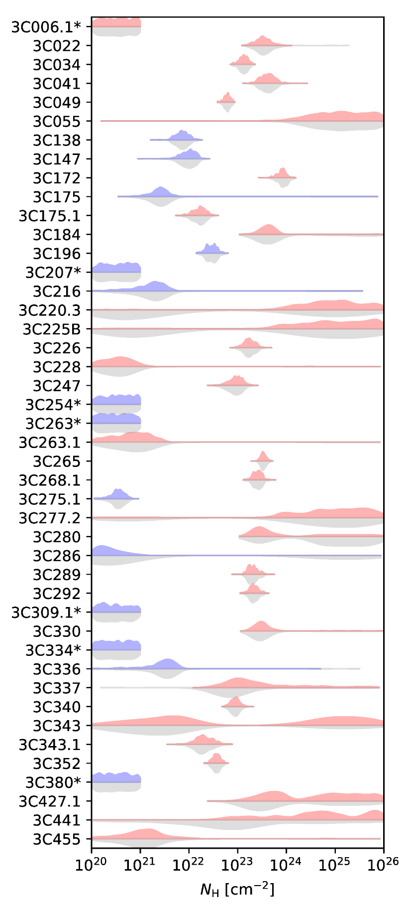
Figure 3: Constraints on the intrinsic column density $N_{\rm H}$ for each source in the sample from the Hierarchical Bayesian Modeling (HBM). Gray distributions show probabilities when assuming (as a first step of the HBM) flat, uninformative priors. Results with posterior probabilities (after incorporating information from the whole sample) are shown in blue for quasars and in red for NLRGs. Thicker vertical dimension of contours implies higher probability. Sources with substantial pileup, marked with an asterisk, were manually given an unobscured ($N_{\rm H}$$<10^{21}$ cm^-2) solution.

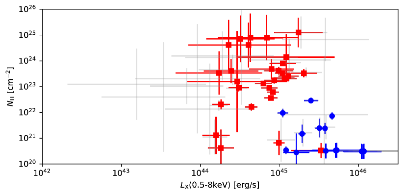
Figure 5: Intrinsic X-ray luminosity $L(0.5-8~{}{\rm keV})$ versus intrinsic column density $N_{\rm H}$ from the Hierarchical Bayesian Modeling (HBM). Results of the first HBM run which assumed flat, uninformative priors are plotted in gray. Results with posterior probabilities (after incorporating information from the whole sample) are plotted in blue for quasars and red in NLRGs. The HBM is able to tighten the constraints on several low-information sources. The few quasars with substantial pileup, which were manually set to be unobscured with $N_{\rm H}$ $<10^{21}$ cm^-2 have luminosities $>10^{45.5}$ erg s^-1.

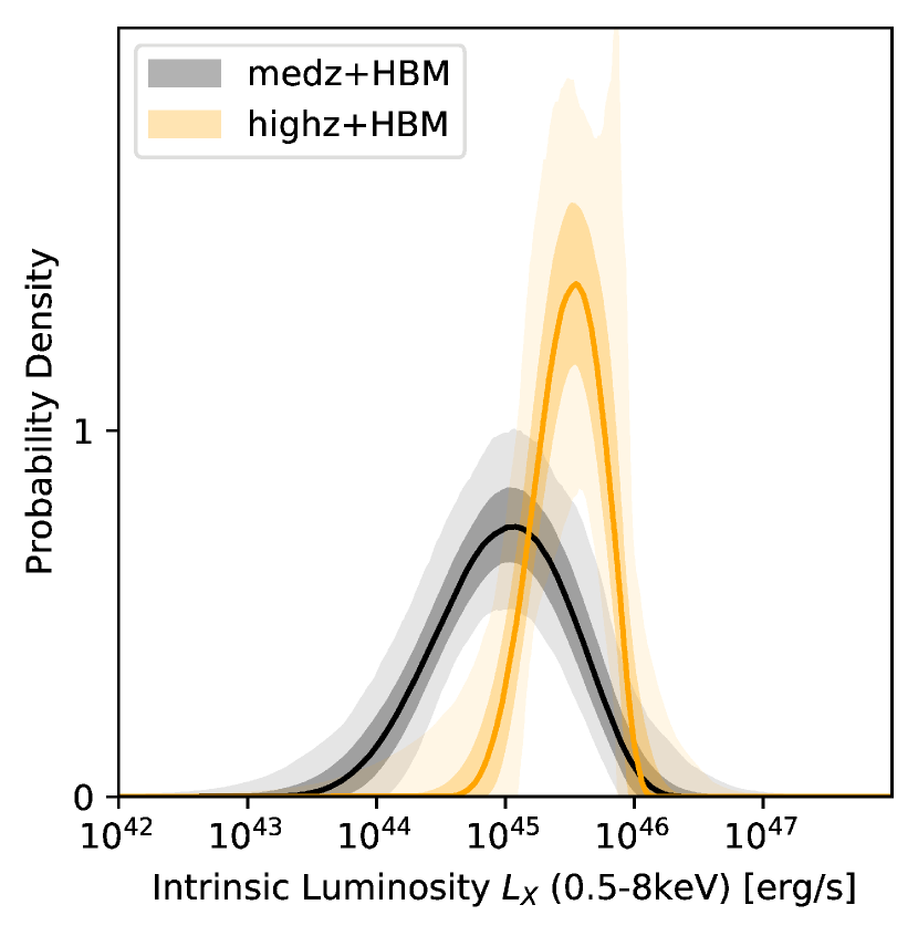
Figure 18: Intrinsic 0.5–8 keV luminosity distributions of the medium-redshift (gray) and high-redshift (yellow) population derived from the HBM modeling of the two samples. The high-luminosity tail ($L_{\rm X}>10^{46}$ erg s^-1) of the medium-$z$ sample is due to a simplistic treatment of a few piled-up quasars for which $N_{\rm H}$ $<10^{21}$ cm^-2 was assumed. Shaded areas give 68% and 99% confidence intervals.

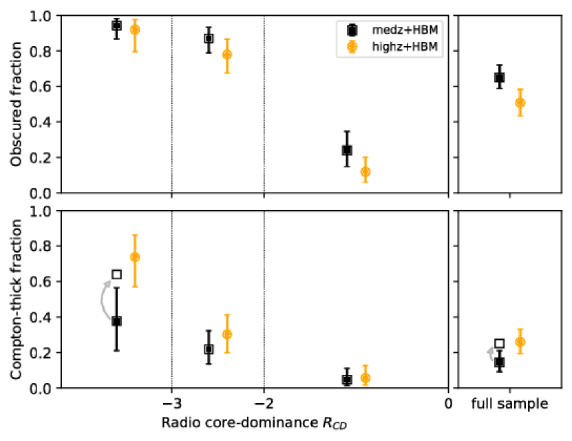
Figure 19: The total obscured ($N_{\rm H}$ $>10^{22}$ cm^-2) fraction (top) and Compton-thick ($N_{\rm H}$ $>10^{24}$ cm^-2) fraction (bottom) from the Hierarchical Bayesian modeling. Fractions are shown in three bins of log $R_{\rm CD}$ (three left-most pairs of panels) showing an increase with inclination. Fractions for the full medium-$z$ and high-$z$ samples are shown in the right-most pair of panels. Open squares indicate Compton-thick fractions estimated from multiwavelength data (Section 7.4).

9 Appendix

9.1 Hierarchical Bayesian Model

Inference on the obscured fraction in this sample is challenging because of substantial uncertainties of measurements. For several observations, short exposures give large uncertainties on the line-of-sight obscuration, which can additionally be degenerate with the intrinsic AGN luminosity. We want to incorporate these uncertainties to produce realistic estimates of the obscured fraction. A self-consistent framework to do this is a Hierarchical Bayesian Model (HBM). We begin by writing down Bayes theorem for an individual object:

$$p(\theta|D)=\frac{p(D|\theta)\times p(\theta)}{p(D)}$$

The posterior probability distribution $p(\theta|D)$ of the parameters $\theta=(L_{\rm{X}},{N_{\rm{H}}})$ is primarily shaped by the likelihood function $p(D|\theta)$, given by the Poisson count probability (Cash, 1979) comparing the detected counts $c_{i}$ to the assumed X-ray spectral model $m_{i}$ propagated through the detector response:

$$p(D|\theta)=\prod_{i}\rm{Poisson}(c_{i};m_{i}(\theta))$$

The second ingredient is $p(\theta)$, which normally is the prior of the Bayesian computation, describing the prior knowledge of the parameters $\theta$. In a Hierarchical Bayesian Model, we estimate $p(\theta)$ simultaneously from the observations themselves.

To this end, we define only the shape of $p(\theta)$ assuming population distributions with hyper-parameters (parameters of the prior distribution) $H$:

$$p(\theta,H)=p(L_{\rm{X}},H)\times p({N_{\rm{H}}},H)$$

As an example, the population distribution could be described by Gaussian distributions whose parameters would be the hyper-parameters H.

For the column density ${N_{\rm{H}}}$ we assume a log-uniform distribution within three bins (“unobscured” $20-22$, “Compton-thin obscured”, $22-24$ and “Compton-thick”, $24-26$). The relative ratio is defined by the obscured fraction, $f_{\rm{obsc}}$ and the fraction of obscured AGN that are Compton-thick, $f_{\rm{CT}}$:

$$p({N_{\rm{H}}},f_{\rm{obsc}},f_{\rm{CT}})=\left\{\begin{array}[]{ll}1-f_{\rm{obsc}}&\rm{if\,}{N_{\rm{H}}}<10^{22}\rm{cm}^{-2}\\ f_{\rm{obsc}}\times(1-f_{\rm{CT}})&\rm{if\,}{N_{\rm{H}}}=10^{22-24}\rm{cm}^{-2}\\ f_{\rm{CT}}&\rm{if\,}{N_{\rm{H}}}>10^{24}\rm{cm}^{-2}\end{array}\right.$$

For the luminosity distribution we adopt the flexible Beta distribution (adopting a Gaussian or Student-t distribution instead does not change the results significantly):

$$p(L_{\rm{X}},\mu,\sigma,a,b)=\rm{Beta}(\log L_{X};\mu,\sigma,a,b)\times p(\mu,\sigma,a,b).$$

For the population hyper-parameters, we adopt a uniform prior on the mean logarithmic luminosity $\mu$, a log-uniform prior on the population dispersion scale $\sigma$ and uniform priors on the shape parameters $a$ and $b$.

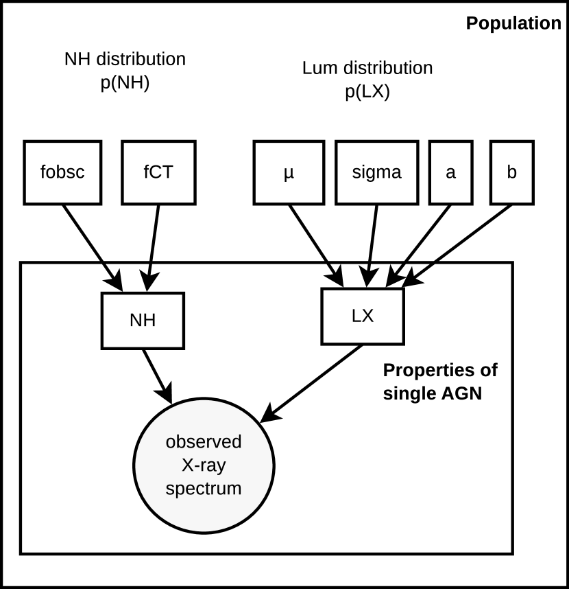
Figure 20: Hierarchical Bayesian model. The circle indicates observations and rectangles indicate parameters. In the top half, a population distribution with some hyper-parameters $(\mu,\sigma)$ generated AGN with some properties ($L_{\rm{X}}$, ${N_{\rm{H}}}$). In the bottom half, these in turn generated the observed X-ray spectral data. The Hierarchical Bayesian model quantifies the probability of this multi-level process as a function of its parameters.

We can then estimate the parameters $\theta$ for all sources (their $L_{\rm{X}}$, ${N_{\rm{H}}}$) simultaneously with the hyper-parameters $H=(f_{\rm{obsc}},f_{\rm{CT}},\mu,\sigma,a,b)$. That means, we explore a $(6+N\times 2)$-dimensional parameter space:

$$p(H,\theta_{0},\theta_{1}...,\theta_{N})=\prod_{i}p(D|\theta_{i})\times p(\theta_{i},H)$$

and as usual in Bayesian inference, derive marginalized probability distributions on the physical parameters (e.g., ${N_{\rm{H}}}$), but also the population distribution in ${N_{\rm{H}}}$.

In this analysis, the source parameters influence the population distributions. At the same time, if the population distribution is well-constrained by the majority of sources, a source with poor observational constraints can benefit from the population distribution, as it gives a prior where the parameters are most likely. Thus, the Hierarchical Bayesian Model strengthens weak observations (the population informs inference of individual objects down the hierarchy) and allows inference of the population distribution (individual objects inform the population distribution up the hierarchy). The model is illustrated in Figure 20.

In practice, we compute the hierarchical model in two steps. First, we compute $p(\theta_{i}|D)$ for each object under uninformative (flat) priors. This is a simple X-ray spectral analysis with the BXA (Bayesian X-ray Analysis; Buchner et al., 2014) module for Sherpa (Fruscione et al., 2006), assuming an AGN with obscuration (BNTORUS model; Brightman & Nandra, 2011) with a warm, mirror power law added (similar to the scattered AGN light component in Section 4.4). All normalizations have wide log-uniform (uninformative) priors, the intrinsic photon index is assigned a Gaussian prior centered at $1.95$ with standard deviation $0.15$. The warm mirror normalization can reach up to $10\%$ of the intrinsic AGN powerlaw component. This standard setup is described e.g. in Buchner et al. (2014). The X-ray spectral analysis produces posterior distributions in $p(\theta_{i}|D)$ that are described by equally probable posterior samples $\theta_{ij}$ (as may be familiar from Markov chain Monte Carlo analyses). In our case, we select $M=1000$ posterior samples for each source. These samples cluster where the posterior is most probable, and thus can be used as weight points in Monte Carlo integrations.

To constrain the population parameters, we then evaluate the population distribution at the object posterior sample locations:

$$p(H)=\prod_{i}\frac{1}{M}\sum_{j}p(\theta_{ij},H)$$

and only need to explore a 6-dimensional parameter space. This is well-defined because the $\theta_{ij}$ samples indicate where the population distributions have most weight. If the samples from one object are clustered distant from another object’s samples, then the population distribution must spread to cover both. On the other hand, because the population distribution is a probability distribution normalised to unity, extremely wide distributions give low probabilities at any specific location. Therefore the population distribution will prefer to cover the samples. If uncertainties (cluster widths) become large, both narrow and broad population distributions are similarly probable. Thereby, this formalism self-consistently carries forward the uncertainties from each source analysis into the uncertainties on population parameters.

9.2 Object constraints with flat population priors

We first analyze the spectra of sources independently with BXA and report the ${N_{\rm{H}}}$ and $L_{\rm{X}}$ constraints under flat priors. The probability distributions of ${N_{\rm{H}}}$ and $L_{\rm{X}}$ for each source are presented in Figure 3 and 4 respectively, as gray contours.

We correct for significantly piled-up ($>20\%$) sources, where naive spectral analysis may be biased by assuming these are unobscured luminous AGN, in the following way. We assume a log-uniform column density probability $\log{N_{\rm{H}}}=20-21$. For the luminosity distribution, we take lower limit of the luminosity derived from spectral analysis as a lower limit on the true luminosity, and assume a log-uniform distribution extending to very high luminosities ($\log L_{\rm X}=\log L_{\rm X,min}-47$). The population model will truncate the high-luminosity end based on other sources (see Figure 3 and 4, where gray shapes show probability distributions from spectral analysis, and red shapes show updated probability distributions after reweighing by the HBM analysis). This suppresses the extremely high luminosities of the piled-up sources (marked with an asterisk), and some Compton-thick, high-luminosity secondary solutions (e.g. in 3C184 and 3C280) based on the Compton-thick fractions of the well-constrained (by HBM) sources.

Figure 5 shows the constraints on both the luminosity and column density for all sources in the medium-$z$ 3CRR sample.

9.3 HBM constraints

We now use the HBM to estimate the intrinsic luminosity distribution and the obscured fractions of the population. The luminosity distribution for the medium-$z$ 3CRR sample is shown in red in Figure 18. It is centered at $\mu=45.1\pm 1.2$ and $\sigma=4.5\pm 1.0$ wide. The shape of the distribution is described by $a=7.7\pm 1.8$ and $b=3.6\pm 2.6$, indicating a right-skewed, steeply falling distribution.

We perform the same analysis for the high-$z$ 3CRR sample analysed in Wilkes et al. (2013) and find consistent results in the spectral analysis and reported obscured and Compton-thick fractions. The X-ray luminosity distribution for the high-$z$ sample is shown in black in Figure 18.

Finally, to investigate the dependence of obscured and Compton-thick fractions on orientation (i.e. $R_{\rm CD}$), we modify the HBM to allow three different groups (log $R_{\rm CD}$$<-3$ , $-3<$ log $R_{\rm CD}$ $<-2$ , $-2<$ log $R_{\rm CD}$$<0$) to have different obscured fractions, while still enforcing the same luminosity distribution for all groups. The results are presented in Figure 19, with the total obscured fraction in the top panels, and the Compton-thick fraction in the bottom panels. The obscured fraction increases to $>70\%$ for more intermediate and edge-on viewing angles (log $R_{CD}<-2$). It is remarkably low ($\lesssim 20\%$) for face-on sources. The Compton-thick fraction is small until the lowest log $R_{CD}<-3$ values are reached; in those edge-on sources it reaches $\tilde{6}0\%$. Within the uncertainties, the obscuration results from the two samples are consistent with each other.

The obscured fractions are shown in Figure 19. We obtain an upper limit on the Compton-thick fraction of all AGN in both medium- and high-$z$ samples of 20% and an obscured fraction of $55\pm 10\%$. The low Compton-thick fraction (found from the HBM) is due to the few secure Compton-thick candidates (see Figure 5). However when information from multiwavelength data is included in estimating the number of CT sources (Section 7.4) - the CT fractions for the medium-$z$ sample and the most edge-on inclination sources (log $R_{\rm CD}$ $<-3$) increases and approaches those found for the high-$z$ sample. All obscured and CT fractions, derived with the HBM, are listed in Table 7.

Table 7: Obscured fractions derived with the HBM.

	Obscured fraction	Compton-thick fraction
	Medium-z Sample:
full sample	$0.57^{+0.09}_{+0.08}$	$0.07^{+0.07}_{+0.04}$
$-2<$ log $R_{\rm CD}$ $<0$	$0.19^{+0.11}_{+0.08}$	$0.05^{+0.07}_{+0.04}$
$-3<$ log $R_{\rm CD}$ $<-2$	$0.81^{+0.08}_{+0.11}$	$0.11^{+0.12}_{+0.07}$
log $R_{\rm CD}$ $<-3$	$0.92^{+0.05}_{+0.10}$	$0.34^{+0.21}_{+0.17}$
	High-z Sample:
full sample	$0.51^{+0.08}_{+0.07}$	$0.26^{+0.07}_{+0.06}$
$-2<$ log $R_{\rm CD}$ $<0$	$0.12^{+0.08}_{+0.06}$	$0.06^{+0.07}_{+0.04}$
$-3<$ log $R_{\rm CD}$ $<-2$	$0.78^{+0.09}_{+0.10}$	$0.30^{+0.11}_{+0.10}$
log $R_{\rm CD}$$<-3$	$0.92^{+0.06}_{+0.12}$	$0.74^{+0.12}_{+0.17}$

References

- Aird et al. (2015) Aird, J., Alexander, D. M., Ballantyne, D. R., et al. 2015, ApJ, 815, 66
- Akujor & Garrington (1995) Akujor, C. E., & Garrington, S. T. 1995, A&AS, 112, 235
- Aldcroft et al. (1994) Aldcroft, T. L., Bechtold, J., & Elvis, M. 1994, ApJS, 93, 1
- Alexander et al. (2003) Alexander, D. M., Bauer, F. E., Brandt, W. N., et al. 2003, AJ, 126, 539
- An & Baan (2012) An, T., & Baan, W. A. 2012, ApJ, 760, 77
- Antonucci (1993) Antonucci, R. 1993, ARA&A, 31, 473
- Baldwin et al. (1973) Baldwin, J. A., Burbidge, E. M., Hazard, C., et al. 1973, ApJ, 185, 739
- Barmby et al. (2006) Barmby, P., Alonso-Herrero, A., Donley, J. L., et al. 2006, ApJ, 642, 126
- Barthel (1989) Barthel, P. D. 1989, ApJ, 336, 606
- Barthel et al. (1990) Barthel, P. D., Tytler, D. R., & Thomson, B. 1990, A&AS, 82, 339
- Belsole et al. (2006) Belsole, E., Worrall, D. M., & Hardcastle, M. J. 2006, MNRAS, 366, 339
- Belsole et al. (2007) Belsole, E., Worrall, D. M., Hardcastle, M. J., & Croston, J. H. 2007, MNRAS, 381, 1109
- Bennett et al. (2014) Bennett, C. L., Larson, D., Weiland, J. L., & Hinshaw, G. 2014, ApJ, 794, 135
- Bogers et al. (1994) Bogers, W. J., Hes, R., Barthel, P. D., & Zensus, J. A. 1994, A&AS, 105, 91
- Bondi et al. (2004) Bondi, M., Brunetti, G., Comastri, A., & Setti, G. 2004, MNRAS, 354, L43
- Bridle et al. (1994) Bridle, A. H., Hough, D. H., Lonsdale, C. J., Burns, J. O., & Laing, R. A. 1994, AJ, 108, 766
- Brightman & Nandra (2011) Brightman, M., & Nandra, K. 2011, MNRAS, 413, 1206
- Brunetti et al. (2002) Brunetti, G., Bondi, M., Comastri, A., & Setti, G. 2002, A&A, 381, 795
- Buchner et al. (2014) Buchner, J., Georgakakis, A., Nandra, K., et al. 2014, A&A, 564, A125
- Burlon et al. (2011) Burlon, D., Ajello, M., Greiner, J., et al. 2011, ApJ, 728, 58
- Burtscher et al. (2016) Burtscher, L., Davies, R. I., Graciá-Carpio, J., et al. 2016, A&A, 586, A28
- Cash (1979) Cash, W. 1979, ApJ, 228, 939
- Cheung (2004) Cheung, C. C. 2004, PhD thesis, BRANDEIS UNIVERSITY
- Chiaberge et al. (2002) Chiaberge, M., Capetti, A., & Celotti, A. 2002, A&A, 394, 791
- Cleary et al. (2007) Cleary, K., Lawrence, C. R., Marshall, J. A., Hao, L., & Meier, D. 2007, ApJ, 660, 117
- Crawford & Fabian (2003) Crawford, C. S., & Fabian, A. C. 2003, MNRAS, 339, 1163
- Croston et al. (2005) Croston, J. H., Hardcastle, M. J., Harris, D. E., et al. 2005, ApJ, 626, 733
- Cutri et al. (2002) Cutri, R. M., Nelson, B. O., Francis, P. J., & Smith, P. S. 2002, in Astronomical Society of the Pacific Conference Series, Vol. 284, IAU Colloq. 184: AGN Surveys, ed. R. F. Green, E. Y. Khachikian, & D. B. Sanders, 127
- Czerny et al. (1996) Czerny, B., Witt, H. J., & Zycki, P. T. 1996, arXiv e-prints, astro
- Davis et al. (2007) Davis, M., Guhathakurta, P., Konidaris, N. P., et al. 2007, ApJ, 660, L1
- Dennett-Thorpe et al. (1999) Dennett-Thorpe, J., Bridle, A. H., Laing, R. A., & Scheuer, P. A. G. 1999, MNRAS, 304, 271
- Dickey & Lockman (1990) Dickey, J. M., & Lockman, F. J. 1990, ARA&A, 28, 215
- Donahue et al. (2003) Donahue, M., Daly, R. A., & Horner, D. J. 2003, ApJ, 584, 643
- Douglas et al. (1996) Douglas, J. N., Bash, F. N., Bozyan, F. A., Torrence, G. W., & Wolfe, C. 1996, AJ, 111, 1945
- Eisenhardt et al. (2004) Eisenhardt, P. R., Stern, D., Brodwin, M., et al. 2004, ApJS, 154, 48
- Elitzur (2012) Elitzur, M. 2012, ApJ, 747, L33
- Evans et al. (2006) Evans, D. A., Worrall, D. M., Hardcastle, M. J., Kraft, R. P., & Birkinshaw, M. 2006, ApJ, 642, 96
- Ezhikode et al. (2017) Ezhikode, S. H., Gandhi, P., Done, C., et al. 2017, MNRAS, 472, 3492
- Fabian et al. (2008) Fabian, A. C., Vasudevan, R. V., & Gandhi, P. 2008, MNRAS, 385, L43
- Falcke et al. (1995) Falcke, H., Gopal-Krishna, & Biermann, P. L. 1995, A&A, 298, 395
- Fanaroff & Riley (1974) Fanaroff, B. L., & Riley, J. M. 1974, MNRAS, 167, 31P
- Fanti et al. (1985) Fanti, C., Fanti, R., Parma, P., Schilizzi, R. T., & van Breugel, W. J. M. 1985, A&A, 143, 292
- Fanti et al. (1989) Fanti, C., Fanti, R., Parma, P., et al. 1989, A&A, 217, 44
- Fernini et al. (1993) Fernini, I., Burns, J. O., Bridle, A. H., & Perley, R. A. 1993, AJ, 105, 1690
- Fernini et al. (1997) Fernini, I., Burns, J. O., & Perley, R. A. 1997, AJ, 114, 2292
- Freeman et al. (2001) Freeman, P., Doe, S., & Siemiginowska, A. 2001, in Society of Photo-Optical Instrumentation Engineers (SPIE) Conference Series, Vol. 4477, Astronomical Data Analysis, ed. J.-L. Starck & F. D. Murtagh, 76–87
- Fruscione et al. (2006) Fruscione, A., McDowell, J. C., Allen, G. E., et al. 2006, in Society of Photo-Optical Instrumentation Engineers (SPIE) Conference Series, Vol. 6270, Observatory Operations: Strategies, Processes, and Systems
- Gambill et al. (2003) Gambill, J. K., Sambruna, R. M., Chartas, G., et al. 2003, A&A, 401, 505
- Gelderman & Whittle (1994) Gelderman, R., & Whittle, M. 1994, ApJS, 91, 491
- Georgantopoulos et al. (2011) Georgantopoulos, I., Dasyra, K. M., Rovilos, E., et al. 2011, A&A, 531, A116
- Ghisellini & Celotti (2001) Ghisellini, G., & Celotti, A. 2001, A&A, 379, L1
- Ghisellini et al. (1993) Ghisellini, G., Padovani, P., Celotti, A., & Maraschi, L. 1993, ApJ, 407, 65
- Giavalisco et al. (2004) Giavalisco, M., Ferguson, H. C., Koekemoer, A. M., et al. 2004, ApJ, 600, L93
- Gilbert et al. (2004) Gilbert, G. M., Riley, J. M., Hardcastle, M. J., et al. 2004, MNRAS, 351, 845
- Gilli et al. (2007) Gilli, R., Comastri, A., & Hasinger, G. 2007, A&A, 463, 79
- Giovannini et al. (1988) Giovannini, G., Feretti, L., Gregorini, L., & Parma, P. 1988, A&A, 199, 73
- Goulding et al. (2012) Goulding, A. D., Alexander, D. M., Bauer, F. E., et al. 2012, ApJ, 755, 5
- Granato et al. (1997) Granato, G. L., Danese, L., & Franceschini, A. 1997, ApJ, 486, 147
- Gregory & Condon (1991) Gregory, P. C., & Condon, J. J. 1991, ApJS, 75, 1011
- Grimes et al. (2004) Grimes, J. A., Rawlings, S., & Willott, C. J. 2004, MNRAS, 349, 503
- Grimes et al. (2005) —. 2005, MNRAS, 359, 1345
- Grogin et al. (2011) Grogin, N. A., Kocevski, D. D., Faber, S. M., et al. 2011, ApJS, 197, 35
- Haas et al. (2008) Haas, M., Willner, S. P., Heymann, F., et al. 2008, ApJ, 688, 122
- Haas et al. (2014) Haas, M., Leipski, C., Barthel, P., et al. 2014, ApJ, 790, 46
- Hagen et al. (1995) Hagen, H. J., Groote, D., Engels, D., & Reimers, D. 1995, A&AS, 111, 195
- Haggard et al. (2010) Haggard, D., Green, P. J., Anderson, S. F., et al. 2010, ApJ, 723, 1447
- Hardcastle et al. (2002) Hardcastle, M. J., Birkinshaw, M., Cameron, R. A., et al. 2002, ApJ, 581, 948
- Hardcastle et al. (2009) Hardcastle, M. J., Evans, D. A., & Croston, J. H. 2009, MNRAS, 396, 1929
- Hardcastle et al. (2004) Hardcastle, M. J., Harris, D. E., Worrall, D. M., & Birkinshaw, M. 2004, ApJ, 612, 729
- Hardcastle & Worrall (1999) Hardcastle, M. J., & Worrall, D. M. 1999, MNRAS, 309, 969
- Harris & Krawczynski (2006) Harris, D. E., & Krawczynski, H. 2006, ARA&A, 44, 463
- Hasinger (2008) Hasinger, G. 2008, A&A, 490, 905
- Hickox et al. (2007) Hickox, R. C., Jones, C., Forman, W. R., et al. 2007, ApJ, 671, 1365
- Hönig et al. (2010) Hönig, S. F., Kishimoto, M., Gandhi, P., et al. 2010, A&A, 515, A23
- Hough & Readhead (1989) Hough, D. H., & Readhead, A. C. S. 1989, AJ, 98, 1208
- Huchra & Burg (1992) Huchra, J., & Burg, R. 1992, ApJ, 393, 90
- Hutchings et al. (1994) Hutchings, J. B., Neff, S. G., Weadock, J., et al. 1994, AJ, 107, 471
- Jackson & Rawlings (1997) Jackson, N., & Rawlings, S. 1997, MNRAS, 286, 241
- Juneau et al. (2011) Juneau, S., Dickinson, M., Alexander, D. M., & Salim, S. 2011, ApJ, 736, 104
- Just et al. (2007) Just, D. W., Brandt, W. N., Shemmer, O., et al. 2007, ApJ, 665, 1004
- Kim et al. (2007) Kim, M., Kim, D.-W., Wilkes, B. J., et al. 2007, ApJS, 169, 401
- Kuehr et al. (1981) Kuehr, H., Witzel, A., Pauliny-Toth, I. I. K., & Nauber, U. 1981, A&AS, 45, 367
- Kuraszkiewicz et al. (2009a) Kuraszkiewicz, J., Wilkes, B. J., Schmidt, G., et al. 2009a, ApJ, 692, 1180
- Kuraszkiewicz et al. (2009b) —. 2009b, ApJ, 692, 1143
- Kuraszkiewicz et al. (2003) Kuraszkiewicz, J. K., Wilkes, B. J., Hooper, E. J., et al. 2003, ApJ, 590, 128
- La Franca et al. (2005) La Franca, F., Fiore, F., Comastri, A., et al. 2005, ApJ, 635, 864
- Lacy et al. (2004) Lacy, M., Storrie-Lombardi, L. J., Sajina, A., et al. 2004, ApJS, 154, 166
- Laing & Peacock (1980) Laing, R. A., & Peacock, J. A. 1980, MNRAS, 190, 903
- Laing et al. (1983) Laing, R. A., Riley, J. M., & Longair, M. S. 1983, MNRAS, 204, 151
- Laurent-Muehleisen et al. (1997) Laurent-Muehleisen, S. A., Kollgaard, R. I., Ryan, P. J., et al. 1997, A&AS, 122, 235
- Lawrence (1991) Lawrence, A. 1991, MNRAS, 252, 586
- Lawrence & Elvis (1982) Lawrence, A., & Elvis, M. 1982, ApJ, 256, 410
- Lawrence et al. (1996) Lawrence, C. R., Zucker, J. R., Readhead, A. C. S., et al. 1996, ApJS, 107, 541
- Leipski et al. (2010) Leipski, C., Haas, M., Willner, S. P., et al. 2010, ApJ, 717, 766
- Lonsdale et al. (2003) Lonsdale, C. J., Smith, H. E., Rowan-Robinson, M., et al. 2003, PASP, 115, 897
- Ludke et al. (1998) Ludke, E., Garrington, S. T., Spencer, R. E., et al. 1998, MNRAS, 299, 467
- Luo et al. (2015) Luo, B., Brandt, W. N., Hall, P. B., et al. 2015, ApJ, 805, 122
- Ma et al. (1998) Ma, C., Arias, E. F., Eubanks, T. M., et al. 1998, AJ, 116, 516
- Maiolino et al. (2001) Maiolino, R., Marconi, A., Salvati, M., et al. 2001, A&A, 365, 28
- Maiolino & Rieke (1995) Maiolino, R., & Rieke, G. H. 1995, ApJ, 454, 95
- Marchese et al. (2012) Marchese, E., Della Ceca, R., Caccianiga, A., et al. 2012, A&A, 539, A48
- Marin & Antonucci (2016) Marin, F., & Antonucci, R. 2016, ApJ, 830, 82
- Massaro et al. (2011) Massaro, F., Harris, D. E., & Cheung, C. C. 2011, ApJS, 197, 24
- Massaro et al. (2018) Massaro, F., Missaglia, V., Stuardi, C., et al. 2018, ApJS, 234, 7
- Matt et al. (1997) Matt, G., Guainazzi, M., Frontera, F., et al. 1997, A&A, 325, L13
- McCarthy et al. (1997) McCarthy, P. J., Miley, G. K., de Koff, S., et al. 1997, ApJS, 112, 415
- Merloni et al. (2014) Merloni, A., Bongiorno, A., Brusa, M., et al. 2014, MNRAS, 437, 3550
- Miller et al. (2011) Miller, B. P., Brandt, W. N., Schneider, D. P., et al. 2011, ApJ, 726, 20
- Mulchaey et al. (1994) Mulchaey, J. S., Koratkar, A., Ward, M. J., et al. 1994, ApJ, 436, 586
- Mullin et al. (2006) Mullin, L. M., Hardcastle, M. J., & Riley, J. M. 2006, MNRAS, 372, 113
- Mushotzky et al. (1993) Mushotzky, R. F., Done, C., & Pounds, K. A. 1993, ARA&A, 31, 717
- Nenkova et al. (2008a) Nenkova, M., Sirocky, M. M., Ivezić, Ž., & Elitzur, M. 2008a, ApJ, 685, 147
- Nenkova et al. (2008b) Nenkova, M., Sirocky, M. M., Nikutta, R., Ivezić, Ž., & Elitzur, M. 2008b, ApJ, 685, 160
- Netzer (2015) Netzer, H. 2015, ARA&A, 53, 365
- Ni et al. (2018) Ni, Q., Brandt, W. N., Luo, B., et al. 2018, MNRAS, 480, 5184
- Nicastro (2000) Nicastro, F. 2000, ApJ, 530, L65
- O’Dea (1998) O’Dea, C. P. 1998, PASP, 110, 493
- Ogle et al. (2006) Ogle, P., Whysong, D., & Antonucci, R. 2006, ApJ, 647, 161
- Ogle et al. (2003) Ogle, P. M., Brookings, T., Canizares, C. R., Lee, J. C., & Marshall, H. L. 2003, A&A, 402, 849
- Oliver et al. (2012) Oliver, S. J., Bock, J., Altieri, B., et al. 2012, MNRAS, 424, 1614
- Ordovás-Pascual et al. (2017) Ordovás-Pascual, I., Mateos, S., Carrera, F. J., et al. 2017, MNRAS, 469, 693
- Orr & Browne (1982) Orr, M. J. L., & Browne, I. W. A. 1982, MNRAS, 200, 1067
- Panessa & Bassani (2002) Panessa, F., & Bassani, L. 2002, A&A, 394, 435
- Panessa et al. (2006) Panessa, F., Bassani, L., Cappi, M., et al. 2006, A&A, 455, 173
- Park et al. (2010) Park, S. Q., Barmby, P., Willner, S. P., et al. 2010, ApJ, 717, 1181
- Park et al. (2006) Park, T., Kashyap, V. L., Siemiginowska, A., et al. 2006, ApJ, 652, 610
- Pearson & Readhead (1981) Pearson, T. J., & Readhead, A. C. S. 1981, ApJ, 248, 61
- Pearson & Readhead (1988) —. 1988, ApJ, 328, 114
- Petrov et al. (2006) Petrov, L., Kovalev, Y. Y., Fomalont, E. B., & Gordon, D. 2006, AJ, 131, 1872
- Petrov & Taylor (2011) Petrov, L., & Taylor, G. B. 2011, AJ, 142, 89
- Pier & Krolik (1992) Pier, E. A., & Krolik, J. H. 1992, ApJ, 401, 99
- Podigachoski et al. (2015) Podigachoski, P., Barthel, P. D., Haas, M., et al. 2015, A&A, 575, A80
- Polletta et al. (2006) Polletta, M. d. C., Wilkes, B. J., Siana, B., et al. 2006, ApJ, 642, 673
- Ricci et al. (2017) Ricci, C., Trakhtenbrot, B., Koss, M. J., et al. 2017, Nature, 549, 488
- Richards et al. (2003) Richards, G. T., Hall, P. B., Vand en Berk, D. E., et al. 2003, AJ, 126, 1131
- Risaliti et al. (1999) Risaliti, G., Maiolino, R., & Salvati, M. 1999, ApJ, 522, 157
- Sambruna et al. (2004) Sambruna, R. M., Gambill, J. K., Maraschi, L., et al. 2004, ApJ, 608, 698
- Sazonov et al. (2012) Sazonov, S., Willner, S. P., Goulding, A. D., et al. 2012, ApJ, 757, 181
- Schwartz et al. (2004) Schwartz, D. A., Silverman, J., Birkinshaw, M., et al. 2004, ApJ, 605, L105
- Scoville et al. (2007) Scoville, N., Aussel, H., Brusa, M., et al. 2007, ApJS, 172, 1
- Shang et al. (2011) Shang, Z., Brotherton, M. S., Wills, B. J., et al. 2011, ApJS, 196, 2
- Shi et al. (2010) Shi, Y., Rieke, G. H., Smith, P., et al. 2010, ApJ, 714, 115
- Siebenmorgen et al. (2015) Siebenmorgen, R., Heymann, F., & Efstathiou, A. 2015, A&A, 583, A120
- Singal (1993) Singal, A. K. 1993, MNRAS, 263, 139
- Smith et al. (1979) Smith, H. E., Junkkarinen, V. T., Spinrad, H., Grueff, G., & Vigotti, M. 1979, ApJ, 231, 307
- Spinrad et al. (1985) Spinrad, H., Marr, J., Aguilar, L., & Djorgovski, S. 1985, PASP, 97, 932
- Stalevski et al. (2012) Stalevski, M., Fritz, J., Baes, M., Nakos, T., & Popović, L. Č. 2012, MNRAS, 420, 2756
- Stern et al. (2005) Stern, D., Eisenhardt, P., Gorjian, V., et al. 2005, ApJ, 631, 163
- Tavecchio et al. (2005) Tavecchio, F., Cerutti, R., Maraschi, L., et al. 2005, ApJ, 630, 721
- Tran (2003) Tran, H. D. 2003, ApJ, 583, 632
- Treister & Urry (2006) Treister, E., & Urry, C. M. 2006, ApJ, 652, L79
- Trippe et al. (2010) Trippe, M. L., Crenshaw, D. M., Deo, R. P., et al. 2010, ApJ, 725, 1749
- Urry & Padovani (1995) Urry, C. M., & Padovani, P. 1995, PASP, 107, 803
- Véron-Cetty & Véron (2006) Véron-Cetty, M. P., & Véron, P. 2006, A&A, 455, 773
- Werner et al. (2004) Werner, M. W., Roellig, T. L., Low, F. J., et al. 2004, ApJS, 154, 1
- Westhues et al. (2016) Westhues, C., Haas, M., Barthel, P., et al. 2016, AJ, 151, 120
- Wilkes & Elvis (1987) Wilkes, B. J., & Elvis, M. 1987, ApJ, 323, 243
- Wilkes et al. (2005) Wilkes, B. J., Pounds, K. A., Schmidt, G. D., et al. 2005, ApJ, 634, 183
- Wilkes et al. (2002) Wilkes, B. J., Schmidt, G. D., Cutri, R. M., et al. 2002, ApJ, 564, L65
- Wilkes et al. (2012) Wilkes, B. J., Lal, D. V., Worrall, D. M., et al. 2012, ApJ, 745, 84
- Wilkes et al. (2013) Wilkes, B. J., Kuraszkiewicz, J., Haas, M., et al. 2013, ApJ, 773, 15
- Willott et al. (1999) Willott, C. J., Rawlings, S., Blundell, K. M., & Lacy, M. 1999, MNRAS, 309, 1017
- Willott et al. (2000) —. 2000, MNRAS, 316, 449
- Wills & Brotherton (1995) Wills, B. J., & Brotherton, M. S. 1995, ApJ, 448, L81
- Worrall (2009) Worrall, D. M. 2009, A&A Rev., 17, 1
- Worrall et al. (1987) Worrall, D. M., Giommi, P., Tananbaum, H., & Zamorani, G. 1987, ApJ, 313, 596
- Worrall & Wilkes (1990) Worrall, D. M., & Wilkes, B. J. 1990, ApJ, 360, 396
- Wright (2006) Wright, E. L. 2006, PASP, 118, 1711
- Wu et al. (2012) Wu, X.-B., Hao, G., Jia, Z., Zhang, Y., & Peng, N. 2012, AJ, 144, 49
- Zacharias & Zacharias (2014) Zacharias, N., & Zacharias, M. I. 2014, AJ, 147, 95
- Zakamska et al. (2005) Zakamska, N. L., Schmidt, G. D., Smith, P. S., et al. 2005, AJ, 129, 1212
- Zamorani et al. (1981) Zamorani, G., Henry, J. P., Maccacaro, T., et al. 1981, ApJ, 245, 357
- Zhu et al. (2020) Zhu, S. F., Brandt, W. N., Luo, B., et al. 2020, MNRAS, 496, 245