Stochastic partial differential equations arising in self-organized criticality

Abstract

We study scaling limits of the weakly driven Zhang and the Bak-Tang-Wiesenfeld (BTW) model for self-organized criticality. We show that the weakly driven Zhang model converges to a stochastic partial differential equation (PDE) with singular-degenerate diffusion. In addition, the deterministic BTW model is shown to converge to a singular-degenerate PDE. Alternatively, the proof of the scaling limit can be understood as a convergence proof of a finite-difference discretization for singular-degenerate stochastic PDEs. This extends recent work on finite difference approximation of (deterministic) quasilinear diffusion equations to discontinuous diffusion coefficients and stochastic PDEs. In addition, we perform numerical simulations illustrating key features of the considered models and the convergence to stochastic PDEs in spatial dimension $d=1,2$.

MSC 2010: 46B50, 60H15, 65M06

Keywords: Self-organized criticality, scaling limits, explicit finite difference approximation, weak convergence approach, singular-degenerate SPDEs

1 Introduction

The concept of self-organized criticality (SOC) was introduced by Bak, Tang and Wiesenfeld in the seminal articles [2, 3] by means of the paradigmatic “sandpile model”. This particle model serves as a guiding example of a non-equilibrium system reaching criticality without apparent external tuning of model parameters, thus exemplifying the concept of SOC. The field of SOC has since received strong interest in physics and alternative particle models like the Zhang model have been introduced, see for example [83, 75, 36, 71, 87, 48, 67, 1, 24, 33]. Despite their apparent simplicity, the analysis of the dynamics of these sandpile models is challenging and the microscopic models contain several arbitrary degrees of freedom, such as the structure of the underlying grid and its size. Consequently, already shortly after the introduction of the concept of SOC, continuum models mimicking the discrete systems have been introduced in the physics literature, see e. g. [38, 34, 23, 75, 76, 55, 37, 25, 69, 57, 20, 22, 58, 77, 49]. Informally, these are thought to correspond to continuum limits of the discrete systems (1.2), (1.5), leading to singular-degenerate stochastic partial differential equations (SPDEs) of the type

$$\begin{split}\mathrm{d}X(t)&=\Delta\tilde{\phi}(X(t))\mathrm{d}t+B(X(t))\mathrm{d}W(t)\quad\text{on }(0,T]\times(0,1).\\ \end{split}$$ (1.1)

Motivated by this development, a large number of mathematical contributions have been devoted to the analysis of such (stochastic) PDEs, see, for example, [7, 6, 17, 8, 5, 11, 9, 10, 16, 12, 15, 13, 14, 28, 27, 80, 81, 53, 51]. However, despite the ongoing interest in continuum models for SOC, so far their rigorous justification in terms of scaling limits of the discrete systems remained an open problem. As a consequence, also the question in which scaling regimes these continuum models apply remained unanswered.

The goal of the present work is to address the aforementioned open problems: We identify scaling regimes for the model parameters $D$ and $\sigma^{2}$ in (1.5) for which the rescaled weakly driven Zhang model converges to the solution of a singular stochastic PDE of the type (1.1). The proof of this fact is challenging due to the interplay of the irregularity of the random forcing, which converges to space-time white noise, with the degeneracy of the diffusion. For this reason, a proof based on distribution spaces taking the place of more classic function spaces has to be developed. In addition, we prove that the pure diffusion part of the BTW model converges to a deterministic, singular-degenerate PDE. In this case, an additional difficulty arises due to the non-reflexivity of the corresponding energy space. This is overcome in the present work by devising an SVI approach for this setting.

The “sandpile model”, also called BTW model in the following, specifies the evolution of the height $(X^{n,j})_{n=0,\dots,N;j\in\Lambda}\subset\mathbb{R}$ of a number of particles on a $d$-dimensional grid $j\in\Lambda=\{0,\dots,Z\}^{d}$ of length $Z\in\mathbb{N}_{\geq 2}$ in discrete time $n\in\{0,1,\dots,N\}$, $N\in\mathbb{N}$. The dynamics of the height are induced by a competition of energy input and dissipation: As long as a critical height $K$ is not exceeded, that is $\|X^{n,\cdot}\|_{\infty}\leq K$, energy is added to the system. If the critical height $K$ is exceeded, the dissipation mechanism, a so-called toppling event, is invoked redistributing energy throughout the system. Without loss of generality, $K$ can be set to $1$ by a scaling argument. This leads to the definition of the dynamics via

$$X^{n+1,j}=X^{n,j}+D\sum_{j^{\prime}\sim j}\left(\tilde{\phi}(X^{n,j^{\prime}})-\tilde{\phi}(X^{n,j})\right)+\mathds{1}_{\{\|X^{n,\cdot}\|_{\infty}\leq 1\}}\xi^{n,j},$$ (1.2)

for $j\in\Lambda^{\prime}=\{1,\dots,Z-1\}^{d}$, where the sum reaches over direct neighboring cells $j^{\prime}$ of $j$, $D\in\big{(}0,\frac{1}{2d}\big{]}$, $\tilde{\phi}=\tilde{\phi}_{1}$ with

$$\tilde{\phi}_{1}(x)=\mathds{1}_{(1,\infty)}(x)-\mathds{1}_{(-\infty,-1)}(x),$$ (1.3)

and $\xi^{n,j}=\tilde{\mu}\delta_{j,s_{n}}$, $\tilde{\mu}>0$, are random variables with $s_{n}\sim\mathrm{Uni}(\Lambda^{\prime})$ independently identically distributed. By fixing the height to zero on $\Lambda\setminus\Lambda^{\prime}$, energy can be dissipated via toppling.

Subsequently, several modifications of the original BTW model have been introduced, for example, the Zhang model for which the diffusion $\tilde{\phi}=\tilde{\phi}_{2}$ takes the form

$$\tilde{\phi}_{2}(x)=|x|\left(\mathds{1}_{(1,\infty)}(x)-\mathds{1}_{(-\infty,-1)}(x)\right),$$ (1.4)

among many more, see, for example [71, 44]. Both models share the properties to be slowly driven by energy input with rapid relaxation, that have been identified in [36, Section III.1] as characteristics of systems displaying SOC.

Following [36, Section III.2], we introduce the weakly driven BTW/Zhang models

$$X^{n+1,j}=X^{n,j}+D\sum_{j^{\prime}\sim j}\left(\tilde{\phi}(X^{n,j^{\prime}})-\tilde{\phi}(X^{n,j})\right)+\xi^{n,j},$$ (1.5)

where now $(\xi^{n,j})_{n=0,\dots,N;j\in\Lambda^{\prime}}$ are independent random variables identically distributed with positive mean $\mathbb{E}\xi^{n,j}=\tilde{\mu}>0$ and finite variance $\mathrm{Var}\left(\xi^{n,j}\right)=\sigma^{2}<\infty$. We call these models weakly driven, since the totally asymmetric noise in (1.2), which only takes non-negative values, is replaced by a weakly asymmetric noise which still has positive mean, but may also take negative values.

Starting from the zero initial condition, energy builds up in the system until toppling events appear. These can induce chain reactions, that is, cause subsequent topplings. A series of $m$ toppling events is called an avalanche of size $m$. A key observation in SOC is that the systems described above reach criticality, in the sense that the statistics of the sizes of avalanches show a power law behavior (see e. g. [3]). The numerical simulations presented in Section 4.2 below demonstrate that this behavior is still present in the weakly asymmetric case (1.5).

More precisely, with the space-time rescaling $h=\frac{1}{Z},\tau=\frac{T}{N}$, model (1.5) becomes

$$\begin{split}X_{h,\tau}^{n+1,\cdot}&=X_{h,\tau}^{n,\cdot}+\tau\Delta_{h}\tilde{\phi}\left(X_{h,\tau}^{n,\cdot}\right)+\tilde{\xi}_{h,\tau}^{n,\cdot},\quad\text{for }n=0,\dots,N-1,\\ X_{h,\tau}^{0}&=x_{h}^{0},\end{split}$$ (1.6)

with zero boundary condition, where the random variables $(\tilde{\xi}_{h,\tau}^{n,j})_{j\in\Lambda^{\prime}}$ are assumed to be $\mathbb{R}$-valued, independent identically distributed with mean $\mu\tau$, variance $\frac{\tau}{h^{d}}$ and finite sixth moments. This scaling means that the constants $D$, $\tilde{\mu}$ and $\sigma^{2}$ in (1.5) are replaced by $\frac{\tau}{h^{2}}=\frac{TZ^{2}}{N}$, $\tau\mu=\frac{\mu T}{N}$ and $\frac{\tau}{h^{d}}=\frac{TZ^{d}}{N}$, respectively. Furthermore, $\Delta_{h}$ denotes the discrete Dirichlet Laplacian. Recall that on the level of the discrete model, $D$ encodes the share of the quantity on the critical site being redistributed during one toppling event, and $\mu$ encodes the average quantity added in each time step.

In the following, we identify grid functions on the lattice $h\Lambda^{\prime}$ with their prolongations chosen to be piecewise affine in time and piecewise constant in space.

Theorem 1.1 (See Theorem 2.3 below).

Let $d=1$. Consider the rescaled weakly driven Zhang model (1.6) with diffusion nonlinearity $\phi_{2}$ and initial condition $x^{0}_{h}\in\mathbb{R}^{Z-1}$. Assume that that the (strong) CFL condition

$$\frac{\tau}{h^{2}}\to 0\quad\text{for }\tau,h\to 0$$ (1.7)

is satisfied and that $x_{h}^{0}\to x_{0}\in L^{2}([0,1])$ for $h\to 0$. Then,

$$X_{h,\tau}\to X\quad\text{in }L^{2}([0,T];L^{2}([0,1])\text{ and }L^{\infty}([0,T];{H^{-1}})$$

for $\tau,h\to 0$ in distribution, where $X$ is the unique weak solution to

$$\begin{split}\mathrm{d}X(t)&=\Delta\tilde{\phi}_{2}(X(t))\,\mathrm{d}t+\mu\mathrm{d}t+\mathrm{d}W(t)\quad\text{on }(0,T]\times(0,1),\\ X(0)&=x_{0},\end{split}$$ (1.8)

with initial state $x_{0}\in L^{2}([0,1])$ and $W$ is a cylindrical $\mathrm{Id}$-Wiener process on $L^{2}([0,1])$.

While the Zhang model and the BTW model share the difficulty of a discontinuous and locally degenerate diffusion, the diffusivity of the BTW model also degenerates for large values. This complicates the mathematical analysis. In this case, the convergence of the purely diffusive part can still be obtained.

Theorem 1.2 (See Theorem 3.3 below).

Consider the BTW model without external forcing and let $d=1$. Assume that (1.7) is satisfied and that $x_{h}^{0}\to x_{0}$ in $L^{2}([0,1])$ for $h\to 0$. Then,

$$X_{h,\tau}\to X\quad\text{weakly* in }L^{\infty}([0,T];{H^{-1}})$$

for $\tau,h\to 0$, where $X$ is the unique EVI solution to

$$\begin{split}\mathrm{d}X(t)&=\Delta\tilde{\phi}_{1}(X(t))\,\mathrm{d}t\quad\text{on }(0,T]\times(0,1),\\ X(0)&=x_{0},\end{split}$$ (1.9)

with initial state $x_{0}\in L^{2}([0,1])$.

The above two main results can be reinterpreted in terms of the convergence of time explicit finite difference schemes for singular-degenerate (stochastic) PDE. From this viewpoint, the results presented in this work partially extend those of the recent contribution [32]. More precisely, the results of [32] in particular imply the convergence of explicit finite difference schemes of singular-degenerate PDE of the type (1.1) with $B\equiv 0$ and Lipschitz continuous nonlinearities $\tilde{\phi}$. Due to the discontinuous nature of the diffusion coefficients (1.3), (1.4) the results of [32] are not applicable in the present setting. In addition, the arguments developed in [43, 32] rely on compactness arguments in $L^{1}$, and, therefore, require at least $L^{1}$ regularity for the forcing. In the context of stochastic PDE considered here, these methods are not applicable, since (1+1)-dimensional space-time white noise has spatial regularity only $\mathcal{C}^{-\frac{1}{2}-}$. Therefore, arguments applicable in spaces of distributions have to be developed, which is done in the present work by establishing an $H^{-1}$-based approach rather than working in $L^{1}$.

In the language of numerical analysis, the first main result obtained in this work and, analogously, the second one can be re-formulated as follows.

Corollary 1.3.

Let $d=1$. Consider a rectangular grid covering $[0,T]\times[0,1]$ with grid size $h$ and time step size $\tau$ and assume that (1.7) is satisfied. Then, the solutions of the explicit finite difference discretization of the stochastic PDE (1.8), i.e., (1.6) with $\tilde{\phi}=\tilde{\phi}_{2}$, converge for $\tau,h\to 0$ to the unique weak solution of (1.8) in the same sense as in Theorem 1.1.

Remark 1.4.

The proof in [32] relies on a comparison principle on the level of the discrete scheme, which is closely connected to the CFL-type condition

$$\frac{\tau}{h^{2}}\leq\frac{1}{2d\,\mathrm{Lip}_{\tilde{\phi}}},$$

where $\mathrm{Lip}_{\tilde{\phi}}$ is the Lipschitz constant of the nonlinearity ${\tilde{\phi}}$ (see [32, p. 2272]). Due to the discontinuous nature of the nonlinearities in (1.3) and (1.4) such a condition can only be satisfied in a limiting sense, thus motivating (1.7).

In Section 4, numerical simulations are included going beyond the above setup for which rigorous results are obtained, by investigating rates of convergence, convergence in stronger topologies, and relaxed assumptions. For example, numerical simulations for $d=2$ are included indicating the existence of a non-trivial limit for the Zhang and BTW model (1.6). Notably, in higher spatial dimension $d\geq 2$, the regularity of space-time white noise and, thus, of solutions to (1.8) becomes worse and renormalization may become necessary.

We conclude the introduction with some brief comments on the method of proof: The proof of convergence is based on a compactness argument and thus fundamentally relies on establishing uniform energy estimates on the discrete solutions. In order to establish these estimates, we introduce discrete analogs of the continuous $H^{-1}$ norm, where the continuous Laplacian $\Delta$ is replaced by its discrete counterpart $\Delta_{h}$. This allows to reproduce the known continuous energy estimates on the discrete level, but leads to discretization dependent norms and spaces. The discrete stability estimates are then carefully transferred to spatially continuous interpolants of the discrete solutions. The derived estimates provide the basis for the subsequent compactness arguments based on the “weak convergence approach” inspired by [46]. The identification of the resulting limit as a probabilistically weak solution to the stochastic PDE driven by space-time white noise is challenging, due to its multivalued nature, but can be resolved by monotonicity techniques, as long as the corresponding energy space is reflexive. This finishes the proof for the Zhang model. The monotonicity approach fails in the case of the BTW nonlinearity, since weak convergence can only be obtained in weaker topologies due to the non-reflexivity of the energy space. At this point the solution concept of stochastic variational inequalities (SVI solutions) proves crucial as it does not rely on reflexivity. This approach allows to conclude the convergence of the discrete BTW model in the deterministic setting.

The structure of this paper is as follows: We first give an overview on the mathematical and physical literature in Section 1.1 and introduce some general notational conventions in Section 1.2. The continuum limits of the weakly driven Zhang and BTW model are then treated in Section 2 and Section 3, respectively. Numerical experiments are included in Section 4.

1.1 Mathematical literature

We first mention previous attempts to approach SOC in a continuous setting. Related to the scaling limit approach, one strategy consists in considering cellular automata resulting from a reformulation and modification of the original sandpile models, as proceeded in [24], in order to obtain a problem which is more accessible for analysis. For one of these models, a hydrodynamic limit PDE has been rigorously obtained in [25]. Scaling limits of the SOC models introduced above have been asserted in [38, 34, 75, 6, 7, 22]. For the existence of a scaling limit for deterministic sandpiles started from specific initial configurations, we refer to [74]. In [78, 20, 57], systems of PDEs are analyzed as ad-hoc models for natural processes displaying power-law statistics.

The analysis of the scaling behavior of SOC particle models leads to questions also arising in the analysis of explicit finite difference discretizations of (generalized) porous media equations. The latter has been subject to a lively research activity in numerical mathematics, advancing from the classical power functions (e. g. [35]) via differentiable nonlinearities ([43]) to merely Lipschitz nonlinearities ([32]). As related results, we mention convergence results for implicit finite difference schemes of degenerate porous media equations ([42, 32]) and a finite-difference discretization of a fractional porous medium equation ([31]).

Regarding the numerical approximation of probabilistically weak solutions of nonlinear SPDEs we refer to the overview paper [72] and the references therein. For discretizations of stochastic porous media equations, we refer to [54], where an $L^{2}$ based finite element approach is applied in order to construct and analyze solutions for sufficiently smooth noise as well as to the recent work [19] that employs an $H^{-1}$ based finite element approach which also covers the case of space-time white noise for $d=1$. In [50, 56], linear SPDEs with multiplicative noise are discretized using finite difference approximations in space, while [68] considers space-time finite difference approximations of linear parabolic SPDEs with additive noise. To the best of the authors’ knowledge, the present work is the first time that finite difference approximations of stochastic porous media equations are rigorously analyzed.

Concerning the underlying techniques the main arguments of this article rely on, we mention the following sources of theory and inspiration. For Yamada-Watanabe type results, we refer to [85] for the foundational work and to [63, 79] for applications to SPDEs. The meanwhile classical weak convergence approach has been used previously, e. g. , by [45, 21, 52, 29], relying on a Skorohod-type result by Jakubowski [60]. For the identification of the limit of the discrete approximations as a solution, we use the theory of maximal monotone operators given e. g. in [4] in a similar way as [66], and a generalized Donsker-type invariance principle given in [40].

1.2 Notation

Let $\mathcal{O}\subset\mathbb{R}^{d}$, $d\in\mathbb{N}$, be an open and bounded set. For $k\geq 0$, let $\mathcal{C}^{k}(\mathcal{O})$ ($\mathcal{C}_{c}^{k}(\mathcal{O})$) be the space of $k$ times continuously differentiable real-valued functions (with compact support), where the index $k=0$ will be omitted. Similarly, for a Banach space $V$, $\mathcal{C}^{k}([0,T];V)$ denotes be the space of $k$ times continuously differentiable curves in $V$ parametrized by $t\in[0,T]$. Let $L^{2}:=L^{2}(\mathcal{O})$ be the Lebesgue space of square integrable functions, endowed with the norm $\left\lVert\cdot\right\rVert_{L^{2}}$. Let ${H^{1}_{0}}:={H^{1}_{0}}(\mathcal{O})$ be the Sobolev space of weakly differentiable functions with zero trace, endowed with the norm $\left\lVert u\right\rVert_{H^{1}_{0}}=\left\lVert\nabla u\right\rVert_{L^{2}}$, and let ${H^{-1}}$ be its topological dual space. For two separable Hilbert spaces $H_{1}$, $H_{2}$, we write $L_{2}(H_{1},H_{2})$ for the space of all Hilbert-Schmidt operators from $H_{1}$ to $H_{2}$.

We now turn to the finite-dimensional structures which we will use to formulate numerical convergence results. From now on, we fix

$$\mathcal{O}=[0,1]\subset\mathbb{R}.$$

Consider an equidistant grid on the unit interval with grid points $(x_{i})_{i=0}^{Z}$ with $h=\frac{1}{Z},Z\in\mathbb{N}$ and $x_{i}=ih$. For $i=0,\dots,Z-1$ let $y_{i}=\left(i+\frac{1}{2}\right)h$. Consider the sets of intervals $(K_{i})_{i=0,\dots,Z}$ and $(J_{i})_{i=0,\dots,Z-1}$ given by

$$\begin{split}&K_{0}=[x_{0},y_{0}),\ K_{Z}=\left[y_{Z-1},x_{Z}\right],\ K_{i}=[y_{i-1},y_{i})\text{ for }i=1,\dots,Z-1,\\ &J_{i}=[x_{i},x_{i+1})\text{ for }i=0,\dots,Z-1.\end{split}$$ (1.10)

We consider the space of grid functions on $(x_{i})_{i=0}^{Z}$ with zero boundary conditions, which is isomorphic to $\mathbb{R}^{Z-1}$. We write $\mathbf{1}=(1,\dots,1)\in\mathbb{R}^{Z-1}$. We define the following prolongations.

Definition 1.5.

Let $u_{h}=(u_{h,1},\dots,u_{h,Z-1})\in\mathbb{R}^{Z-1}$. We then define the piecewise linear prolongation with respect to the grid $(x_{i})_{i=0,\dots,Z}$ with zero-boundary conditions by

$$I_{h}^{\mathrm{plx}}\,:\mathbb{R}^{Z-1}\hookrightarrow{H^{1}_{0}},\ u_{h}\mapsto{u_{h}^{\text{plx}}}:=\sum_{i=0}^{Z-1}\left[u_{h,i}+\frac{u_{h,i+1}-u_{h,i}}{h}(\cdot-x_{i})\right]\mathds{1}_{J_{i}},$$

using the convention $u_{h,0}=u_{h,Z}=0$, and the piecewise constant prolongation by

$$I_{h}^{\mathrm{pcx}}\,:\mathbb{R}^{Z-1}\hookrightarrow L^{2},\ u_{h}\mapsto{u^{\text{pcx}}}:=\sum_{i=1}^{Z-1}u_{h,i}\mathds{1}_{K_{i}}.$$

The image of $I_{h}^{\mathrm{pcx}}\,$, i. e. the space of piecewise constant functions on the partition $(K_{i})_{i=0}^{Z}$ with zero Dirichlet boundary conditions, will be denoted by ${S_{h}^{\text{pcx}}}$. The $L^{2}$-orthogonal projection to this space will be denoted by ${\Pi_{h}^{\text{pcx}}}$. Note that $I_{h}^{\mathrm{pcx}}\,:\mathbb{R}^{Z-1}\to{S_{h}^{\text{pcx}}}$ is bijective.

Let $\left\langle\cdot,\cdot\right\rangle:=\left\langle\cdot,\cdot\right\rangle_{l^{2}}$ denote the inner product arising from the Euclidean norm $\left\lVert\cdot\right\rVert:=\left\lVert\cdot\right\rVert_{l^{2}}$ on $\mathbb{R}^{Z-1}$. For a matrix $A\in\mathbb{R}^{(Z-1)\times(Z-1)}$, $\left\lVert A\right\rVert$ denotes the matrix norm induced by $\left\lVert\cdot\right\rVert$. Let $\Delta_{h}\in\mathbb{R}^{(Z-1)\times(Z-1)}$ be the matrix corresponding to the finite difference Laplacian on grid functions on $(x_{i})_{i=0}^{Z}$ with zero Dirichlet boundary conditions, i. e.

$$\Delta_{h}=-\frac{1}{h^{2}}\begin{pmatrix}2&-1&&&&\\ -1&2&-1&&\makebox(0.0,10.0)[]{\text{\huge 0}}&\\ &-1&\ddots&\ddots&&\\ &&\ddots&\ddots&-1&\\ &\makebox(0.0,0.0)[]{\text{\huge 0}}&&-1&2&-1\\ &&&&-1&2\end{pmatrix}.$$ (1.11)

Recall that $-\Delta_{h}$ is symmetric and positive definite (for a formal argument, see Lemma B.1 below). Hence, the following definition is admissible.

Definition 1.6.

On $\mathbb{R}^{Z-1}$, we define the inner products $\left\langle\cdot,\cdot\right\rangle_{0}$, $\left\langle\cdot,\cdot\right\rangle_{1}$ and $\left\langle\cdot,\cdot\right\rangle_{-1}$ by

$$\left\langle u,v\right\rangle_{0} =h\left\langle u,v\right\rangle,$$

$$\left\langle u,v\right\rangle_{1} =\left\langle-\Delta_{h}u,v\right\rangle_{0},$$

$$\left\langle u,v\right\rangle_{-1} =\left\langle(-\Delta_{h})^{-1}u,v\right\rangle_{0}$$

for $u,v\in\mathbb{R}^{Z-1}$. The induced norms are denoted by $\left\lVert\cdot\right\rVert_{0},\left\lVert\cdot\right\rVert_{1}$ and $\left\lVert\cdot\right\rVert_{-1}$.

Remark 1.7.

The norm $\left\lVert\cdot\right\rVert_{0}$ in Definition 1.6 corresponds to the $L^{2}$ norm on $\mathcal{O}$ by the fact that

$$I_{h}^{\mathrm{pcx}}\,:\left(\mathbb{R}^{Z-1},\left\lVert\cdot\right\rVert_{0}\right)\to\left({S_{h}^{\text{pcx}}},\left\lVert\cdot\right\rVert_{L^{2}}\right)$$

is an isometry, i. e.

$$\left\langle u,v\right\rangle_{0}=\left\langle I_{h}^{\mathrm{pcx}}\,u,I_{h}^{\mathrm{pcx}}\,v\right\rangle_{L^{2}}\quad\text{for }u,v\in\mathbb{R}^{Z-1}.$$

Furthermore, Definition 1.6 suggests to view $\left\lVert\cdot\right\rVert_{1}$ and $\left\lVert\cdot\right\rVert_{-1}$ as discrete analogs of the ${H^{1}_{0}}$ and ${H^{-1}}$ norms on $\mathcal{O}$, respectively. These connections are more subtle and will be made more precise in Lemma B.4, Lemma B.5 and Proposition B.6 below.

Next, we consider a lattice for the time interval $[0,T]$, $T>0$. For $\tau>0$ such that $T=N\tau$, $N\in\mathbb{N}$, consider the equidistant grid $(0,\tau,2\tau,\dots,N\tau)$. We then define the following prolongations of grid functions.

Definition 1.8.

Let $v=(v_{k})_{k=0}^{N}\subseteq\mathbb{R}$ be a grid function on the previously described grid of length $\tau$ and let $t_{\tau}:=\tau\left\lfloor\frac{t}{\tau}\right\rfloor$. Then we define the piecewise linear prolongation ${v^{\text{plt}}}:[0,T]\to\mathbb{R}$, the left-sided piecewise constant prolongation ${v^{\text{pct-}}}:[0,T]\to\mathbb{R}$ and the right-sided piecewise constant prolongation ${v^{\text{pct+}}}:[0,T]\to\mathbb{R}$ by

$${v^{\text{plt}}}(t)=\frac{t-t_{\tau}}{\tau}v_{\left\lfloor t/\tau\right\rfloor+1}+\frac{t_{\tau}+\tau-t}{\tau}v_{\left\lfloor t/\tau\right\rfloor},\quad{v^{\text{pct-}}}(t)=v_{\left\lfloor t/\tau\right\rfloor},\quad{v^{\text{pct+}}}(t)=v_{\left\lfloor t/\tau\right\rfloor+1}.$$

For space-time grid functions $\left(u_{k,l}\right)_{k=0,\dots,N;l=1,\dots,Z-1}\subset\mathbb{R}$, we define the space-time prolongations ${u^{\text{plt,pcx}}},{u^{\text{pct-pcx}}},{u^{\text{pct+pcx}}}$ by extending both in space and time. Note that it does not matter whether one first carries out the space or the time prolongation.

2 Continuum limit for the weakly driven Zhang model

For the first main result, let $\phi_{2}:\mathbb{R}\to 2^{\mathbb{R}}$ be the maximal monotone extension of

$$\tilde{\phi}_{2}:\mathbb{R}\ni x\mapsto x\,\mathds{1}_{\left|x\right|>1}(x),$$ (2.1)

which is a special case of the Zhang nonlinearity in (1.4). We consider the singular-degenerate stochastic partial differential inclusion

$$\begin{split}\mathrm{d}X(t)&\in\Delta(\phi_{2}(X(t)))+\mu\mathrm{d}t+\mathrm{d}W(t),\\ X(0)&=x_{0},\end{split}$$ (2.2)

on the interval $(0,1)\subset\mathbb{R}$ with zero Dirichlet boundary conditions, where $\mu\geq 0$ and $x_{0}\in L^{2}:=L^{2}((0,1))$. In this setting, $W$ is a cylindrical $\mathrm{Id}$-Wiener process in $L^{2}$. We set the stage for the following analysis by defining a notion of solution to (2.2) in a probabilistically weak sense.

Definition 2.1.

A triple $\left((\tilde{\Omega},\tilde{\mathcal{F}},(\tilde{\mathcal{F}}_{t})_{t\in[0,T]},\tilde{\mathbb{P}}),\tilde{X},\tilde{W}\right)$, where $(\tilde{\Omega},\tilde{\mathcal{F}},(\tilde{\mathcal{F}}_{t})_{t\in[0,T]},\tilde{\mathbb{P}})$ is a complete probability space endowed with a normal filtration,

$$\tilde{X}\in L^{2}\left(\tilde{\Omega}\times[0,T];L^{2}\right)\cap L^{2}\left(\tilde{\Omega};L^{\infty}([0,T];{H^{-1}})\right)$$

is an $(\tilde{\mathcal{F}}_{t})_{t\in[0,T]}$-progressively measurable process and $\tilde{W}$ is a cylindrical $\mathrm{Id}$-Wiener process with respect to $(\tilde{\mathcal{F}}_{t})_{t\in[0,T]}$ in $L^{2}$, is a weak solution to (2.2), if there exists an $(\tilde{\mathcal{F}}_{t})_{t\in[0,T]}$-progressively measurable process $\tilde{Y}\in L^{2}(\tilde{\Omega}\times[0,T];L^{2})$ such that

$$\tilde{X}(t)=x_{0}+\mu t+\int_{0}^{t}\Delta\tilde{Y}(r)\,\mathrm{d}r+\tilde{W}(t)$$ (2.3)

is satisfied in $L^{2}(\tilde{\Omega}\times[0,T];(L^{2})^{\prime})$, and

$$\tilde{Y}(t)\in\phi_{2}(\tilde{X}(t))\quad(\mathrm{d}t\otimes\mathrm{d}x)\text{-almost everywhere }\tilde{\mathbb{P}}\text{-almost surely}.$$ (2.4)

It will be shown in Section A that the processes $(\tilde{X},\tilde{W})$ of every weak solution to (2.2) have the same law with respect to the Borel $\sigma$-algebra of $L^{2}([0,T];L^{2})\times\mathcal{C}([0,T];{H^{-1}})$.

We make the following central assumption for the rest of this article.

Assumption 2.2.

Let $T>0$. We choose sequences $(Z_{m})_{m\in\mathbb{N}},(N_{m})_{m\in\mathbb{N}}\subset\mathbb{N}$ such that, for $h_{m}=\frac{1}{Z_{m}}$, $\tau_{m}=\frac{T}{N_{m}}$ ($m\in\mathbb{N}$),

$$h_{m}\to 0\text{ for }m\to\infty$$

and

$$\frac{\tau_{m}}{h_{m}^{2}}\to 0\quad\text{for }m\to\infty$$ (CFL)

is satisfied, which presents a strengthened Courant-Friedrichs-Lewy-type condition.

Motivated by the discrete Zhang model, we construct a family of time-discrete evolution processes on $\mathbb{R}^{Z_{m}-1}$ as follows. For each $m\in\mathbb{N}$, we define $(X_{h_{m}}^{n})_{n\in\{0,1,\dots,N_{m}+1\}}\subset\mathbb{R}^{Z_{m}-1}$ iteratively by

$$\begin{split}X_{h_{m}}^{n+1}&=X_{h_{m}}^{n}+\tau_{m}\Delta_{h_{m}}\tilde{\phi}_{2}(X_{h_{m}}^{n})+\mu\tau_{m}+\sqrt{\frac{\tau_{m}}{h_{m}}}\xi_{h_{m}}^{n},\quad\text{for }n=0,\dots,N_{m},\\ X_{h_{m}}^{0}&=x_{h_{m}}^{0},\end{split}$$ (2.5)

where $(x_{h_{m}}^{0})_{m\in\mathbb{N}}\subset\mathbb{R}^{Z_{m}-1}$ such that ${(x_{h_{m}}^{0})^{\text{pcx}}}\to x_{0}$ in $L^{2}$, and $(\xi_{h_{m}}^{n,l})_{n=0,\dots,N_{m};l=1,\dots,Z_{m}-1}$ are centered independent random variables identically distributed on a probability triple $(\Omega,\mathcal{F},\mathbb{P})$. We assume that $\mathbb{E}(\xi_{h_{1}}^{0,1})^{2}=1$ and that $\mathbb{E}(\xi_{h_{1}}^{0,1})^{6}$ is finite.

Recall the extensions of grid functions to functions defined in Definition 1.8. We then have the following main result, which will be proved at the end of Section 2.1.

Theorem 2.3.

Recall the notation from Section 1.2, let Assumption 2.2 be satisfied and, for $m\in\mathbb{N}$, consider the process $(X_{h_{m}}^{n})_{n=0}^{N_{m}}$ given by (2.5). Then, for $m\to\infty$, ${X_{h_{m}}^{\text{plt,pcx}}}$ converges in distribution to the unique weak solution to (2.2) with respect to the weak topology on $L^{2}([0,T];L^{2})$ and the weak* topology on $L^{\infty}([0,T];{H^{-1}})$.

2.1 A priori estimates and transfer to extensions

For the rest of this section, we write $\phi=\phi_{2}$ and $\tilde{\phi}=\tilde{\phi}_{2}$, and we drop the index $m$ of the discretization sequences

$$(h_{m})_{m\in\mathbb{N}},(Z_{m})_{m\in\mathbb{N}},(\tau_{m})_{m\in\mathbb{N}},(N_{m})_{m\in\mathbb{N}},$$

writing instead $(h)_{h>0}$ etc. Moreover, the convergence of sequences and usually nonrelabeled subsequences indexed by $m$ for $m\to\infty$ will be denoted by $h\to 0$. Expressions like “for $h>0$” have to be understood in the sense “for all elements of $(h_{m})_{m\in\mathbb{N}}$” or “for all elements of the subsequence at hand”. For $h>0$, we set $(\mathcal{F}_{h}^{n})_{n=0}^{N}$, $\mathcal{F}_{h}^{n}\subseteq\mathcal{F}$, to be the filtration generated by $(\xi_{h}^{k})_{k=0}^{N}$, i. e.

$$\mathcal{F}_{h}^{n}=\sigma\left(\xi_{h}^{k}:k\in\{0,\dots,n-1\}\right)\quad\text{for }n\in\{0,\dots,N\}.$$ (2.6)

We have the following bounds on the discrete process $X_{h}$ defined in (2.5).

Lemma 2.4.

Let $\tau,h>0,Z,N\in\mathbb{N}$ as in Assumption 2.2, where we choose $h$ small enough for $\tau<1$ and $\frac{\tau}{h^{2}}\leq\frac{1}{12}$ to be satisfied. Then, the discrete process in (2.5) satisfies

$$\begin{split}\left\lVert X_{h}^{n}\right\rVert_{-1}^{2}+\mathcal{S}_{n,h}&\leq\left\lVert x_{h}^{0}\right\rVert_{-1}^{2}+\sum_{k=0}^{n-1}\bigg{(}2\sqrt{\frac{\tau}{h}}\left\langle X_{h}^{k},\xi_{h}^{k}\right\rangle_{-1}+C\tau\\ &\quad+2\tau^{\frac{3}{2}}h^{-\frac{1}{2}}\left\langle\Delta_{h}\tilde{\phi}(X_{h}^{k})+\mu\mathbf{1},\xi_{h}^{k}\right\rangle_{-1}+\frac{\tau}{h}\left\lVert\xi_{h}^{k}\right\rVert_{-1}^{2}\bigg{)}\end{split}$$ (2.7)

and

$$\mathbb{E}\left\lVert X_{h}^{n}\right\rVert_{-1}^{2}+\mathbb{E}\,\mathcal{S}_{n,h}\leq\mathbb{E}\left\lVert x_{h}^{0}\right\rVert_{-1}^{2}+n\tau\,\mathrm{Tr}(-\Delta_{h}^{-1})+n\tau C$$ (2.8)

for all $n\in\{1,\dots,N+1\}$, where

$$\mathcal{S}_{n,h}\in\left\{\tau\sum_{k=0}^{n-1}\left\langle X_{h}^{k},\tilde{\phi}(X_{h}^{k})\right\rangle_{0},\tau\sum_{k=0}^{n-1}\left\lVert\tilde{\phi}(X_{h}^{k})\right\rVert_{0}^{2},\tau\sum_{k=0}^{n-1}\left\lVert X_{h}^{k}\right\rVert_{0}^{2}-n\tau\right\}.$$

Moreover, we have for $n\in\{1,\dots,N\}$

$$\frac{1}{h}\mathbb{E}\left\lVert\xi_{h}^{n}\right\rVert_{-1}^{2}=\mathrm{Tr}(-\Delta_{h}^{-1})$$ (2.9)

and

$$\begin{split}&\mathbb{E}\left\lVert X_{h}^{n}\right\rVert_{-1}^{2}+2\tau\mathbb{E}\sum_{k=0}^{n-1}\left\langle X_{h}^{k},\tilde{\phi}(X_{h}^{k})\right\rangle_{0}\\ &\leq\mathbb{E}\left\lVert x_{h}^{0}\right\rVert_{-1}^{2}+n\tau\,\mathrm{Tr}(-\Delta_{h}^{-1})+2\mu\tau\mathbb{E}\sum_{k=0}^{n-1}\left\langle X_{h}^{k},\mathbf{1}\right\rangle_{-1}\\ &\quad+\frac{5\tau}{h^{2}}\left(\mathbb{E}\left\lVert x_{h}^{0}\right\rVert_{-1}^{2}+T\,\mathrm{Tr}(-\Delta_{h}^{-1})+C\right).\end{split}$$ (2.10)

Proof.

For $n\in\{0,\dots,N\}$, we compute

$$\begin{split}&\left\lVert X_{h}^{n+1}\right\rVert_{-1}^{2}=\left\lVert X_{h}^{n}+\tau\Delta_{h}\tilde{\phi}(X_{h}^{n})+\sqrt{\frac{\tau}{h}}\xi_{h}^{n}+\mu\tau\mathbf{1}\right\rVert_{-1}^{2}\\ &=\left\lVert X_{h}^{n}\right\rVert_{-1}^{2}+2\tau\left\langle X_{h}^{n},\Delta_{h}\tilde{\phi}(X_{h}^{n})\right\rangle_{-1}\\ &\quad+2\mu\tau\left\langle X_{h}^{n},\mathbf{1}\right\rangle_{-1}+\tau^{2}\left\lVert\Delta_{h}\tilde{\phi}(X_{h}^{n})\right\rVert_{-1}^{2}+2\mu\tau^{2}\left\langle\Delta_{h}\tilde{\phi}(X_{h}^{n}),\mathbf{1}\right\rangle_{-1}\\ &\quad+2\sqrt{\frac{\tau}{h}}\left\langle X_{h}^{n},\xi_{h}^{n}\right\rangle_{-1}+2\tau^{\frac{3}{2}}h^{-\frac{1}{2}}\left\langle\Delta_{h}\tilde{\phi}(X_{h}^{n})+\mu\mathbf{1},\xi_{h}^{n}\right\rangle_{-1}\\ &\quad+\frac{\tau}{h}\left\lVert\xi_{h}^{n}\right\rVert_{-1}^{2}+\mu^{2}\tau^{2}\left\lVert\mathbf{1}\right\rVert_{-1}^{2}.\end{split}$$ (2.11)

Towards the first claim, we aim to absorb the terms of the third line of (2.11) up to stably-scaled constants into the term

$$\tau\left\langle X_{h}^{n},\Delta_{h}\tilde{\phi}(X_{h}^{n})\right\rangle_{-1}=-\tau\left\langle X_{h}^{n},\tilde{\phi}(X_{h}^{n})\right\rangle_{0}=-\tau\left\lVert\tilde{\phi}(X_{h}^{n})\right\rVert_{0}^{2}.$$

To this end, using Lemma B.7 in the second step, we compute

$$2\mu\tau\left\langle X_{h}^{n},\mathbf{1}\right\rangle_{-1} \leq 2C\tau\left\lVert X_{h}^{n}\right\rVert_{-1}\left\lVert\mathbf{1}\right\rVert_{-1}\leq 2\tau C\left\lVert X_{h}^{n}\right\rVert_{0}\left\lVert\mathbf{1}\right\rVert_{0}$$

$$\leq 2\tau\left(\frac{3}{2}C+\frac{1}{6}\left\lVert X_{h}^{n}\right\rVert_{0}^{2}\right)\leq 3\tau C+\frac{1}{3}\tau\left\lVert\tilde{\phi}(X_{h}^{n})\right\rVert_{0}^{2},$$

further, by (B.1)

$$\tau^{2}\left\lVert\Delta_{h}\tilde{\phi}(X_{h}^{n})\right\rVert_{-1}^{2}\leq 4\tau\frac{\tau}{h^{2}}\left\lVert\tilde{\phi}(X_{h}^{n})\right\rVert_{0}^{2}\leq\frac{1}{3}\tau\left\lVert\tilde{\phi}(X_{h}^{n})\right\rVert_{0}^{2},$$ (2.12)

and

$$\left|2\mu\tau^{2}\left\langle\Delta_{h}\tilde{\phi}(X_{h}^{n}),\mathbf{1}\right\rangle_{-1}\right|\leq 2C\tau^{2}\left\langle\tilde{\phi}(X_{h}^{n}),\mathbf{1}\right\rangle_{0}\leq 3\tau^{2}C+\frac{1}{3}\tau^{2}\left\lVert\tilde{\phi}(X_{h}^{n})\right\rVert_{0}^{2}.$$ (2.13)

Furthermore, note that by the definition of $\tilde{\phi}$, we have for all $x\in\mathbb{R}^{Z-1}$

$$\left\langle x,\tilde{\phi}(x)\right\rangle_{0}=\left\lVert\tilde{\phi}(x)\right\rVert_{0}^{2}.$$ (2.14)

Applying these estimates to (2.11) yields (2.7) with the first choice for $\mathcal{S}_{n,h}$ by induction.

Now taking the expectation in (2.11), we treat the remaining non-constant terms as follows. Recall the definition of the filtration $(\mathcal{F}_{h}^{n})_{n=0}^{N}$ in (2.6) and note that $X_{h}^{n}$ is $\mathcal{F}_{h}^{n}$-measurable, while $\xi_{h}^{n}$ is independent of $\mathcal{F}_{h}^{n}$. Hence, the two mixed terms on the right-hand side of (2.7) vanish, using the tower property of the conditional expectation. For the second-to-last term, we notice that

$$\frac{\tau}{h}\,\mathbb{E}\left\lVert\xi_{h}^{n}\right\rVert_{-1}^{2}=\frac{\tau}{h}\,\mathbb{E}\left\langle-\Delta_{h}^{-1}\xi_{h}^{n},h\xi_{h}^{n}\right\rangle=\tau\,\mathbb{E}\left\langle-\Delta_{h}^{-1}\xi_{h}^{n},\xi_{h}^{n}\right\rangle=\tau\,\mathrm{Tr}(-\Delta_{h}^{-1}),$$ (2.15)

since for any family $(\xi_{i})_{i=1}^{Z-1}$ of random variables with $\mathbb{E}(\xi_{i}\xi_{j})=\delta_{ij}$ and for any matrix $A\in\mathbb{R}^{(Z-1)\times(Z-1)}$, we have

$$\mathbb{E}\left\langle A\xi,\xi\right\rangle=\mathbb{E}\sum_{i,j=1}^{Z-1}A_{ij}\xi_{j}\xi_{i}=\sum_{i,j=1}^{Z-1}A_{ij}\mathbb{E}(\xi_{j}\xi_{i})=\sum_{i,j=1}^{Z-1}A_{ij}\delta_{ij}=\mathrm{Tr}(A).$$ (2.16)

In particular, (2.9) follows. Collecting all estimates, we conclude by induction that

$$\mathbb{E}\left\lVert X_{h}^{n}\right\rVert_{-1}^{2}+\tau\sum_{k=0}^{n-1}\mathbb{E}\left\langle X_{h}^{n},\tilde{\phi}(X_{h}^{n})\right\rangle_{0}\leq\mathbb{E}\left\lVert x_{h}^{0}\right\rVert_{-1}^{2}+n\tau\,\mathrm{Tr}(-\Delta_{h}^{-1})+n\tau C$$ (2.17)

for $n\in\{0,\dots,N+1\}$, which proves (2.8) for the first choice of $\mathcal{S}_{n,h}$. In view of (2.14), this immediately yields (2.7) and (2.8) for the second choice of $\mathcal{S}_{n,h}$. The relation $\left|\tilde{\phi}(x)\right|^{2}\geq\left|x\right|^{2}-1$ extends these statements to the last choice of $\mathcal{S}_{n,h}$. Using the estimates (2.12) and (2.13) without absorbing the respective terms, taking expectation and summing up, we obtain from (2.11)

$$\mathbb{E}\left\lVert X_{h}^{n}\right\rVert_{-1}^{2}+2\tau\mathbb{E}\sum_{k=0}^{n-1}\left\langle X_{h}^{k},\tilde{\phi}(X_{h}^{k})\right\rangle_{0}$$

$$\leq\mathbb{E}\left\lVert x_{h}^{0}\right\rVert_{-1}^{2}+n\tau\,\mathrm{Tr}(-\Delta_{h}^{-1})+2\tau\mu\,\mathbb{E}\sum_{k=0}^{n-1}\left\langle X_{h}^{k},\mathbf{1}\right\rangle_{-1}$$

$$\quad+\left(\frac{4\tau}{h^{2}}+\frac{\tau}{3}\right)\tau\mathbb{E}\sum_{k=0}^{n-1}\left\lVert\tilde{\phi}(X_{h}^{k})\right\rVert_{0}^{2}+\tau n\tau C.$$

Finally, using that $h\leq 1$ by assumption and (2.8), (2.10) follows. ∎

Lemma 2.5.

Let $\tau,h>0$ and $N,Z\in\mathbb{N}$ as in Assumption 2.2, and let $(X_{h}^{n})_{n=0}^{N}$ be constructed as in (2.5). Then

$$\mathbb{E}\max_{n=0,\dots,N}\left\lVert X_{h}^{n}\right\rVert_{-1}^{2}\leq C,$$

where $C$ is independent of $h$.

Proof.

This follows as an application of the Burkholder-Davis-Gundy inequality in the form of [30, Theorem 1] to the discrete martingales in (2.7). ∎

Lemma 2.6.

Let $\tau,h>0$ as in Assumption 2.2. Then, there exists a constant $C>0$ which only depends on $T$ and $x_{h}^{0}$, such that the discrete process in (2.5) satisfies

$$\mathbb{E}\left\lVert X_{h}^{n+1}-X_{h}^{n}\right\rVert_{-1}^{2}\leq C\frac{\tau}{h^{2}}\quad\text{for all }n\in\{0,\dots,N-1\}.$$

Proof.

We compute

$$\begin{split}&\mathbb{E}\left\lVert X_{h}^{n+1}-X_{h}^{n}\right\rVert_{-1}^{2}=\mathbb{E}\left\lVert\tau\Delta_{h}\tilde{\phi}(X_{h}^{n})+\sqrt{\frac{\tau}{h}}\xi_{h}^{n}+\tau\mu\mathbf{1}\right\rVert_{-1}^{2}\\ &=\mathbb{E}\left\lVert\tau\Delta_{h}\tilde{\phi}(X_{h}^{n})\right\rVert_{-1}^{2}+\frac{\tau}{h}\mathbb{E}\left\lVert\xi_{h}^{n}\right\rVert_{-1}^{2}+\tau^{2}\mu^{2}\left\lVert\mathbf{1}\right\rVert_{-1}^{2}\\ &\quad+2\mathbb{E}\left\langle\tau\Delta_{h}\tilde{\phi}(X_{h}^{n})+\tau\mu\mathbf{1},\sqrt{\frac{\tau}{h}}\xi_{h}^{n}\right\rangle_{-1}+2\tau^{2}\mu\,\mathbb{E}\left\langle\Delta_{h}\tilde{\phi}(X_{h}^{n}),\mathbf{1}\right\rangle_{-1}.\end{split}$$ (2.18)

As in the proof of Lemma 2.4, we have that

$$\mathbb{E}\left\langle\tau\Delta_{h}\phi(X_{h}^{n})+\tau\mu\mathbf{1},\sqrt{\frac{\tau}{h}}\xi_{h}^{n}\right\rangle_{-1}=0$$ (2.19)

by the independence of $\xi_{h}^{n}$ of $\mathcal{F}_{h}^{n}$, where $(\mathcal{F}_{h}^{n})_{n=0}^{N}$ is given as in (2.6). In view of (2.9) and Lemma B.3, one may choose $C$ independent of $h$ satisfying

$$\frac{\tau}{h}\mathbb{E}\left\lVert\xi_{h}^{n}\right\rVert_{-1}^{2}\leq\tau C.$$ (2.20)

Finally, using (2.12) and (2.13), we have

$$\tau^{2}\mathbb{E}\left\lVert\Delta_{h}\tilde{\phi}(X_{h}^{n})\right\rVert_{-1}^{2}+2\tau^{2}\mu\mathbb{E}\left\langle\Delta_{h}\tilde{\phi}(X_{h}^{n}),\mathbf{1}\right\rangle_{-1}\leq C\frac{\tau^{2}}{h^{2}}\mathbb{E}\left\lVert\tilde{\phi}(X_{h}^{n})\right\rVert_{0}^{2}+C\tau^{2},$$

such that we can use Lemma 2.4 and Lemma B.3 to finish (2.18) by

$$\begin{split}\mathbb{E}\left\lVert X_{h}^{n+1}-X_{h}^{n}\right\rVert_{-1}^{2}&\leq C\frac{\tau^{2}}{h^{2}}\sum_{k=0}^{N}\mathbb{E}\left\lVert\tilde{\phi}(X_{h}^{k})\right\rVert_{0}^{2}+\tau C\\ &\leq C\frac{\tau}{h^{2}}\left(\mathbb{E}\left\lVert x_{h}^{0}\right\rVert_{-1}^{2}+T\,\mathrm{Tr}(-\Delta_{h}^{-1})+C\right)\leq C\frac{\tau}{h^{2}},\end{split}$$

as required. ∎

The estimates proved above in the discrete setting can be transferred to the extensions to functions, exploiting Lemma B.5.

Corollary 2.7.

Let $\tau,h>0,N,Z\in\mathbb{N}$ as in Assumption 2.2, with $h$ small enough for $\frac{\tau}{h^{2}}\leq\frac{1}{12}$ to be satisfied, and let $X_{h}$ be constructed as in (2.5). Then, there exists $C>0$ only depending on $T$ (in particular, independent of $h$), such that

$$\max\left\{\mathbb{E}\int_{0}^{T}\left\lVert{X_{h}^{\text{plt,pcx}}}\right\rVert_{L^{2}}^{2}\mathrm{d}t,\,\mathbb{E}\int_{0}^{T}\left\lVert{X_{h}^{\text{pct-pcx}}}\right\rVert_{L^{2}}^{2}\mathrm{d}t,\,\mathbb{E}\int_{0}^{T}\left\lVert{X_{h}^{\text{pct+pcx}}}\right\rVert_{L^{2}}^{2}\mathrm{d}t,\right\} \leq C,$$ (2.21)

$$\mathbb{E}\int_{0}^{T}\left\lVert\tilde{\phi}({X_{h}^{\text{pct-pcx}}})\right\rVert_{L^{2}}^{2}\mathrm{d}t \leq C,$$ (2.22)

$$\text{and}\quad\mathbb{E}\operatorname*{ess\,sup}_{t\in[0,T]}\left\lVert{X_{h}^{\text{plt,pcx}}}\right\rVert_{H^{-1}}^{2} \leq C.$$ (2.23)

Furthermore,

$$\sup_{t\in[0,T]}\mathbb{E}\left\lVert{X_{h}^{\text{plt,pcx}}}(t)-{X_{h}^{\text{pct-pcx}}}(t)\right\rVert_{H^{-1}}^{2},\sup_{t\in[0,T]}\mathbb{E}\left\lVert{X_{h}^{\text{plt,pcx}}}(t)-{X_{h}^{\text{pct+pcx}}}(t)\right\rVert_{H^{-1}}^{2}\leq C\frac{\tau}{h^{2}}.$$

2.2 Extraction of convergent subsequences

Definition 2.8.

Let $(X_{h}^{n})_{n=0}^{N}$ and $(\xi_{h}^{n})_{n=0}^{N}$ be defined as in (2.5). We then define random variables $Y_{h},W_{h}:\Omega\to\mathbb{R}^{(Z-1)(N+1)}$ by

$$Y_{h}=\left(\tilde{\phi}(X_{h}^{n})\right)_{n=0}^{N}\quad\text{and}\quad W_{h}=\left(\sum_{k=0}^{n-1}\sqrt{\frac{\tau}{h}}\xi_{h}^{k}\right)_{n=0}^{N+1}.$$

Furthermore, we define $F_{h}:\Omega\to\mathcal{C}([0,T]\times[0,1])$ to be the spatial antiderivative of ${W_{h}^{\text{plt,pcx}}}$, i. e.

$$F_{h}(t,x)=\int_{0}^{x}{W_{h}^{\text{plt,pcx}}}(t,x^{\prime})\,\mathrm{d}x^{\prime}.$$ (2.24)

Remark 2.9.

Note that $F_{h}$ is continuous in time by the continuity of the piecewise linear prolongation, and absolutely continuous in space, since ${W_{h}^{\text{plt,pcx}}}(t,\cdot)$ is Lebesgue integrable at any time $t\in[0,T]$.

Lemma 2.10.

The distributions of $(F_{h})_{h>0}$ are tight with respect to the strong topology $\tau_{C}$ of $\mathcal{C}([0,T]\times[0,1])$ and converge to the distribution of the Brownian sheet (for a Definition, see [61, p. 1]) in $\mathcal{C}([0,T]\times[0,1])$.

Proof.

If we had defined the spatial extension to be piecewise constant between the lattice points, this statement would have followed immediately from [40, Theorem 7.6]. Indeed, the process considered there could be identified with $F_{h}$. In order to transfer these results to the extension which is piecewise constant around the lattice points, as used in the present work, we exploit the explicit connection between these two extensions. In particular, the uniform continuity used to prove tightness carries over from one extension to the other, and the convergence in law then follows from the convergence of the finite-dimensional distributions of the process in [40] and the fact that the finite-dimensional distributions of the difference of the two extensions converge stochastically to zero. ∎

Corollary 2.7 implies tightness of the distributions of $({X_{h}^{\text{plt,pcx}}})_{h>0}$ with respect to the weak* topology $\tau_{w}^{*}$ of $L^{\infty}([0,T];{H^{-1}})$ by the Banach-Alaoglu theorem, and tightness of the distributions of all processes in Corollary 2.7 with respect to the weak topology $\tau_{w}$ of $L^{2}([0,T];L^{2})$ by separability, reflexivity and the Eberlein-Smulian theorem. As a consequence, we have tightness of the distributions of the family

$$\left(({X_{h}^{\text{plt,pcx}}},{X_{h}^{\text{plt,pcx}}},{X_{h}^{\text{pct-pcx}}},{X_{h}^{\text{pct+pcx}}},{Y_{h}^{\text{pct-pcx}}},F_{h})\right)_{h>0}$$ (2.25)

with respect to the product topology of $(\tau_{w}^{*},\tau_{w},\tau_{w},\tau_{w},\tau_{w},\tau_{C})$, which is a key ingredient to prove the following.

Lemma 2.11.

Let $(X_{h})_{h>0}$, $(Y_{h})_{h>0}$ and $(W_{h})_{h>0}$ be defined as in (2.5) and Definition 2.8, respectively. Then, there is a probability space $(\tilde{\Omega},\tilde{\mathcal{F}},\tilde{\mathbb{P}})$, stochastic processes

$$\tilde{X} \in L^{2}(\tilde{\Omega};L^{\infty}([0,T];{H^{-1}}))\cap L^{2}(\tilde{\Omega};L^{2}([0,T];L^{2}),$$

$$\tilde{Y} \in L^{2}(\tilde{\Omega};L^{2}([0,T];L^{2})),$$

$$\tilde{W} \in L^{2}(\tilde{\Omega};\mathcal{C}([0,T];{H^{-1}})),$$

where $\tilde{W}$ is a cylindrical $\mathrm{Id}$-Wiener process in $L^{2}$, a nonrelabeled subsequence $h\to 0$ such that for each $h$ in this subsequence, there are random variables $\tilde{X}_{h},\tilde{Y}_{h},\tilde{W}_{h}:\tilde{\Omega}\to\mathbb{R}^{(N+1)(Z-1)}$, such that for each $h$ in this subsequence,

$$\mathcal{L}\left((\tilde{X}_{h},\tilde{Y}_{h},\tilde{W}_{h})\right)=\mathcal{L}\left((X_{h},Y_{h},W_{h})\right),$$ (2.26)

$$\begin{split}&\mathcal{L}\left(({\tilde{X}_{h}^{\text{plt,pcx}}},{\tilde{X}_{h}^{\text{plt,pcx}}},{\tilde{X}_{h}^{\text{pct-pcx}}},{\tilde{X}_{h}^{\text{pct+pcx}}},{\tilde{Y}_{h}^{\text{pct-pcx}}},{\tilde{W}_{h}^{\text{plt,pcx}}})\right)\\ &=\mathcal{L}\left(({X_{h}^{\text{plt,pcx}}},{X_{h}^{\text{plt,pcx}}},{X_{h}^{\text{pct-pcx}}},{X_{h}^{\text{pct+pcx}}},{Y_{h}^{\text{pct-pcx}}},{W_{h}^{\text{plt,pcx}}})\right)\end{split}$$ (2.27)

with respect to the product topology of $(\tau_{w}^{*},\tau_{w},\tau_{w},\tau_{w},\tau_{w},\tilde{\tau}_{C})$, and $\tilde{\mathbb{P}}$-almost surely, for $h\to 0$,

$${\tilde{X}_{h}^{\text{plt,pcx}}} \overset{\ast}{\rightharpoonup}\tilde{X}\text{ in }L^{\infty}([0,T];{H^{-1}}),$$

$${\tilde{X}_{h}^{\text{plt,pcx}}} \rightharpoonup\tilde{X},{\tilde{X}_{h}^{\text{pct-pcx}}}\rightharpoonup\tilde{X},{\tilde{X}_{h}^{\text{pct+pcx}}}\rightharpoonup\tilde{X},{\tilde{Y}_{h}^{\text{pct-pcx}}}\rightharpoonup\tilde{Y}\text{ in }L^{2}([0,T];L^{2}),$$

$$\text{and}\quad{\tilde{W}_{h}^{\text{plt,pcx}}} \to\tilde{W}\text{ in }\mathcal{C}([0,T];{H^{-1}}).$$

Proof of Lemma 2.11.

Since this type of result is classical in the framework of the so-called weak convergence approach (see e. g. [46, 45, 21, 29]), we only mention the main steps. First, one applies the Skorohod-type result by Jakubowski ([60, Theorem 2]) to the six-tuple (2.25), which uses the abovementioned tightness. Having obtained corresponding almost surely converging processes $({\tilde{X}_{h}^{\text{plt,pcx}}})_{h>0}$ etc. on a different probability space, we transfer the estimates in Corollary 2.7 to these processes and obtain the suitable integrability of the limits by the Fatou lemma and weak(*) lower-semicontinuity of the norms. Next, we identify the $\tau_{w}$-limits of $({\tilde{X}_{h}^{\text{plt,pcx}}})_{h}$, $({\tilde{X}_{h}^{\text{pct-pcx}}})_{h}$ and $({\tilde{X}_{h}^{\text{pct+pcx}}})_{h}$ using the last part of Corollary 2.7, and we identify this limit with the $\tau_{w}^{*}$-limit of $({\tilde{X}_{h}^{\text{plt,pcx}}})_{h}$ by embedding the respective spaces into the common superspace $L^{2}([0,T];{H^{-1}})$. Passing to the distributional spatial derivative of $(\tilde{F}_{h})_{h}$ and its limit $(\tilde{F})$ provides $({\tilde{W}_{h}^{\text{plt,pcx}}})$ and $\tilde{W}$, where the latter is identified as a cylindrical $\mathrm{Id}$-Wiener process in $L^{2}$ by the fact that $\tilde{F}$ is a Brownian sheet. Finally, one identifies the newly-constructed processes as images of the respective extension operator, using that the projection to the respective finite-dimensional subspace is continuous, and constructs pre-images by applying this projection. ∎

Remark 2.12.

Expected values with respect to $\tilde{\mathbb{P}}$ will be denoted by $\tilde{\mathbb{E}}$.

2.3 Identification of the limit as a solution and proof of Theorem 2.3

We now turn to show that the limit processes belong to a weak solution. As a stochastic basis, we choose $(\tilde{\Omega},\tilde{\mathcal{F}},\tilde{\mathbb{P}})$ endowed with the augmented filtration $(\tilde{\mathcal{F}}_{t})_{t\in[0,T]}$ of $(\tilde{\mathcal{F}}_{t}^{\prime})_{t\in[0,T]}$, where

$$\tilde{\mathcal{F}}_{t}^{\prime}:=\sigma\left(\tilde{X}|_{\tilde{\Omega}\times[0,t]},\tilde{Y}|_{\tilde{\Omega}\times[0,t]},\tilde{W}|_{\tilde{\Omega}\times[0,t]}\right).$$ (2.28)

As typical of the weak convergence approach, we obtain that $\tilde{W}$ is a Wiener process with respect to this basis in the sense of [79, Definition 2.1.12], which is a consequence of the independence of external increments in the discrete dynamics and the continuity of the paths of $\tilde{W}$. We continue by showing that $(\tilde{X},\tilde{Y},\tilde{W})$ satisfy equation (2.3).

Lemma 2.13.

Let $(\tilde{X}_{h},\tilde{Y}_{h},\tilde{W}_{h})$ be the processes from Lemma 2.11. Then,

$${\tilde{X}_{h}^{\text{plt}}}(t)=x_{h}^{0}+\int_{0}^{t}\Delta_{h}{\tilde{Y}_{h}^{\text{pct-}}}(r)\,\mathrm{d}r+{\tilde{W}_{h}^{\text{plt}}}(t)+\mu t\mathbf{1}$$ (2.29)

in $L^{2}([0,T];\mathbb{R}^{Z-1})$, $\tilde{\mathbb{P}}$-almost surely, and the limits in Lemma 2.11 satisfy

$$\tilde{X}(t)=x_{0}+\int_{0}^{t}\Delta\tilde{Y}(r)\mathrm{d}r+\tilde{W}(t)+\mu t$$ (2.30)

in $L^{2}([0,T];(L^{2})^{\prime})$, $\tilde{\mathbb{P}}$-almost surely.

Proof.

Step 1: We first prove (2.29). We note that by construction of the prolongations in use here, (2.29) is equivalent to

$$\tilde{X}_{h}^{n}=x_{h}^{0}+\tau\sum_{k=0}^{n-1}\Delta_{h}\tilde{Y}_{h}^{k}+\tilde{W}_{h}^{n}+n\tau\mu\mathbf{1}$$

for all $n\in\{0,\dots,N\}$, $\tilde{\mathbb{P}}$-almost surely, which is verified by the construction of $(X_{h},Y_{h},W_{h})$ in (2.5) and Definition 2.8, and by the equality of laws in (2.26).

Step 2: We need to show that $\tilde{\mathbb{P}}$-almost surely, for every $\zeta\in L^{2}([0,T];L^{2})$,

$$\begin{split}\int_{0}^{T}\left\langle\tilde{X}(t),\zeta(t)\right\rangle_{(L^{2})^{\prime}\times L^{2}}\mathrm{d}t=\int_{0}^{T}\left\langle x_{0}+\int_{0}^{t}\Delta\tilde{Y}(r)\mathrm{d}r+\tilde{W}(t)+\mu t,\zeta(t)\right\rangle_{(L^{2})^{\prime}\times L^{2}}\mathrm{d}t,\end{split}$$ (2.31)

where $\left\langle u,v\right\rangle_{(L^{2})^{\prime}\times L^{2}}=\left\langle-\Delta^{-1}u,v\right\rangle_{L^{2}}$. In this step, we first show (2.31) for a test function $\zeta$ of the type

$$\zeta=\theta(t)\eta,$$ (2.32)

where $\eta\in L^{2}$ and $\theta\in L^{\infty}([0,T])$. By considering (2.29) and using an approximation $\eta_{h}\in\mathbb{R}^{Z-1}$ such that ${\eta_{h}^{\text{pcx}}}\to\eta$ in $L^{2}$ for $h\to 0$, we obtain

$$\int_{0}^{T}\left\langle{\tilde{X}_{h}^{\text{plt}}}(t),\theta(t)\eta_{h}\right\rangle_{-1}\mathrm{d}t=\int_{0}^{T}\left\langle x_{h}^{0}+\int_{0}^{t}\Delta_{h}{\tilde{Y}_{h}^{\text{pct-}}}(r)\mathrm{d}r+{\tilde{W}_{h}^{\text{plt}}}(t)+\mu t\mathbf{1},\theta(t)\eta_{h}\right\rangle_{-1}\mathrm{d}t$$ (2.33)

$\tilde{\mathbb{P}}$-almost surely. Lemma 2.11 and Proposition B.6 then allow to pass to the limit obtaining (2.31), using dominated convergence for the term including $\tilde{Y}_{h}$.

Step 3: By linearity, (2.31) is also true for linear combinations of test functions $\zeta$ of type (2.32) and thus for every polynomial. Thus, we obtain a $\tilde{\mathbb{P}}$-zero set outside of which (2.31) is satisfied for any polynomial. Using the density of polynomials in $L^{2}([0,T]\times[0,1])$ given by the Stone-Weierstrass theorem, outside this zero set the full statement (2.31) is satisfied by passing to the limit of approximating sequences. ∎

Lemma 2.14.

Let $\tilde{Y}$ and $\tilde{W}$ be constructed as in Lemma 2.11 and define the continuous $(L^{2})^{\prime}$-valued process

$$\tilde{Z}(t):=x_{0}+\int_{0}^{t}\Delta\tilde{Y}(r)\mathrm{d}t+\tilde{W}(t)+\mu t$$

for $t\in[0,T]$. Then, we have

$$\tilde{\mathbb{E}}\left(\sup_{t\in[0,T]}\left\lVert\tilde{Z}(t)\right\rVert_{H^{-1}}^{2}\right)<\infty$$

and

$$\begin{split}&\tilde{\mathbb{E}}\left\lVert\tilde{Z}(t)\right\rVert_{H^{-1}}^{2}+2\,\tilde{\mathbb{E}}\int_{0}^{t}\left\langle\tilde{Z}(r),\tilde{Y}(r)\right\rangle_{L^{2}}\mathrm{d}r\\ &=\left\lVert x_{0}\right\rVert_{H^{-1}}^{2}+t\left\lVert I^{\prime}\right\rVert_{L_{2}(L^{2},{H^{-1}})}^{2}+2\,\tilde{\mathbb{E}}\int_{0}^{t}\left\langle\tilde{Z}(r),\mu\right\rangle_{H^{-1}}\mathrm{d}r,\end{split}$$ (2.34)

where $I^{\prime}:L^{2}\hookrightarrow{H^{-1}}$ is the canonical embedding (cf. Lemma B.3).

Proof.

By Lemma 2.13, we have that $\tilde{X}$ and $\tilde{Z}$ are in the same $\tilde{\mathbb{P}}\otimes\mathrm{d}t$-equivalence class, and by the construction in Lemma 2.11 we know that $\tilde{X}\in L^{2}(\tilde{\Omega}\times[0,T];L^{2})$. Moreover, $\tilde{Y}\in L^{2}(\tilde{\Omega};L^{2}([0,T];L^{2}))$ and progressively measurable with respect to $(\tilde{\mathcal{F}}_{t})_{t\in[0,T]}$ by construction. Thus, Itô’s formula from [79, Theorem 4.2.5] applies, which yields both claims. ∎

Remark 2.15.

By (2.30) and the definition of $\tilde{Z}$ above, we have $\tilde{Z}=\tilde{X}$ in $L^{2}(\tilde{\Omega}\times[0,T];(L^{2})^{\prime})$. Furthermore, we have $\tilde{X}\in L^{2}(\tilde{\Omega}\times[0,T];L^{2})$, such that the injectivity of the embedding $L^{2}\hookrightarrow{H^{-1}}\hookrightarrow(L^{2})^{\prime}$, which carries over to an embedding

$$L^{2}(\tilde{\Omega}\times[0,T];L^{2})\hookrightarrow L^{2}(\tilde{\Omega}\times[0,T];(L^{2})^{\prime}),$$

implies that $\tilde{Z}\in L^{2}(\tilde{\Omega}\times[0,T];L^{2})$ and $\tilde{Z}=\tilde{X}$ in $L^{2}(\tilde{\Omega}\times[0,T];L^{2})$.

In view of (2.4), it remains to inspect the relation of $\tilde{X}$ and $\tilde{Y}$. To this end, we aim to use (2.34) for $\tilde{Z}$ replaced by $\tilde{X}$. Since this is only possible $\mathrm{d}t$-almost surely, we need to use an integrated version of (2.34). The resulting double integral in the second term leads to the following definition, which will be useful in the proof of Lemma 2.18 below.

Definition 2.16.

We define the measure $\mu$ on $[0,T]$ as the measure with density

$$[0,T]\ni t\mapsto T-t$$

with respect to $\mathrm{d}t$, and we write $[0,T]_{\mu}$ for the measure space $([0,T],\mu)$. Let $\mathcal{A}\subset L^{2}(\tilde{\Omega}\times[0,T]_{\mu};L^{2})\times L^{2}(\tilde{\Omega}\times[0,T]_{\mu};L^{2})$ be a multivalued operator (which we identify with its graph by a slight abuse of notation) defined by

$$(X,Y)\in\mathcal{A}\quad\text{if and only if}\quad Y\in\phi(X)\ \text{for almost every }(\tilde{\omega},t,x)\in\tilde{\Omega}\times[0,T]\times[0,1].$$ (2.35)

Remark 2.17.

Similarly to the proof of Lemma A.3, we obtain that the operator $\mathcal{A}$ is maximal monotone.

Lemma 2.18.

Let $h>0$, $({\tilde{X}_{h}^{\text{pct-pcx}}})_{h>0},({\tilde{Y}_{h}^{\text{pct-pcx}}})_{h>0},\tilde{X},\tilde{Y}$ be as in Lemma 2.11. Then

$$\limsup_{h\to 0}\tilde{E}\int_{0}^{T}(T-t)\left\langle{\tilde{X}_{h}^{\text{pct-pcx}}}(t),{\tilde{Y}^{\text{pct-pcx}}}_{h}(t)\right\rangle_{L^{2}}\mathrm{d}t\leq\tilde{\mathbb{E}}\int_{0}^{T}(T-t)\left\langle\tilde{X}(t),\tilde{Y}(t)\right\rangle_{L^{2}}\mathrm{d}t.$$

Proof.

We notice that for $f\in L^{1}([0,T];\mathbb{R})$ or measurable $f\geq 0$, we have by Fubini’s (resp. Tonelli’s) theorem

$$\begin{split}&\int_{0}^{T}\int_{0}^{t}f(r)\mathrm{d}r\mathrm{d}t=\int_{0}^{T}\int_{0}^{T}\mathds{1}_{[0,t]}(r)f(r)\mathrm{d}r\mathrm{d}t\\ &=\int_{0}^{T}f(r)\int_{0}^{T}\mathds{1}_{[r,T]}(t)\mathrm{d}t\mathrm{d}r=\int_{0}^{T}(T-r)f(r)\mathrm{d}r.\end{split}$$ (2.36)

Since, due to Lemma 2.11, $({\tilde{X}_{h}^{\text{pct+pcx}}})_{h>0}$ is bounded in $L^{2}(\tilde{\Omega};L^{2}([0,T];L^{2}))$ uniformly in $h$, and ${\tilde{X}_{h}^{\text{pct+pcx}}}\rightharpoonup\tilde{X}$ $\tilde{\mathbb{P}}$-almost surely in $L^{2}([0,T];L^{2})$, we have

$${\tilde{X}_{h}^{\text{pct+pcx}}}\rightharpoonup\tilde{X}\quad\text{in }L^{2}(\tilde{\Omega};L^{2}([0,T];L^{2}))$$

for $h\to 0$. Hence,we have by weak lower-semicontinuity of the norm that

$$-\tilde{\mathbb{E}}\int_{0}^{T}\left\lVert\tilde{X}(t)\right\rVert_{H^{-1}}^{2}\mathrm{d}t\geq\limsup_{h\to 0}\left(-\tilde{\mathbb{E}}\int_{0}^{T}\left\lVert{\tilde{X}_{h}^{\text{pct+pcx}}}(t)\right\rVert_{H^{-1}}^{2}\mathrm{d}t\right).$$ (2.37)

Furthermore, by the same arguments as in the proof of Proposition B.6, we obtain

$${\left(-\Delta_{h}^{-1}x_{h}^{0})\right)^{\text{pcx}}}\rightharpoonup-\Delta^{-1}x_{0}\quad\text{in }L^{2}\ \text{for }h\to 0,$$

which allows to compute

$$\begin{split}\lim_{h\to 0}\left\lVert x_{h}^{0}\right\rVert_{-1}^{2}=\lim_{h\to 0}\left\langle-\Delta_{h}^{-1}x_{h}^{0},x_{h}^{0}\right\rangle_{0}&=\lim_{h\to 0}\left\langle{(-\Delta_{h}^{-1}x_{h}^{0})^{\text{pcx}}},{(x_{h}^{0})^{\text{pcx}}}\right\rangle_{L^{2}}\\ &=\left\langle-\Delta^{-1}x_{0},x_{0}\right\rangle_{L^{2}}=\left\lVert x_{0}\right\rVert_{H^{-1}}^{2}.\end{split}$$ (2.38)

For each $h>0$ in the subsequence of Lemma 2.11, consider $\tilde{X}_{h}$ and $\tilde{Y}_{h}$ as constructed in Lemma 2.11. Then, by (2.36) and Remark 1.7, we obtain

$$\limsup_{h\to 0}\tilde{\mathbb{E}}\int_{0}^{T}(T-t)\left\langle{\tilde{X}_{h}^{\text{pct-pcx}}}(t),{\tilde{Y}_{h}^{\text{pct-pcx}}}(t)\right\rangle_{L^{2}}\mathrm{d}t$$

$$=\limsup_{h\to 0}\int_{0}^{T}\tilde{\mathbb{E}}\int_{0}^{t}\left\langle{\tilde{X}_{h}^{\text{pct-pcx}}}(r),{\tilde{Y}_{h}(r)^{\text{pct-pcx}}}\right\rangle_{L^{2}}\mathrm{d}r\,\mathrm{d}t$$

$$=\limsup_{h\to 0}\int_{0}^{T}\tilde{\mathbb{E}}\int_{0}^{t}\left\langle{\tilde{X}_{h}^{\text{pct-}}}(s),{\tilde{Y}_{h}^{\text{pct-}}}(s)\right\rangle_{0}\mathrm{d}s\,\mathrm{d}t.$$ (2.39)

Writing $t_{\tau}=\left\lfloor t/\tau\right\rfloor\tau$ and using the definition of the left-sided piecewise constant embedding embedding, the positive sign of $\left\langle{\tilde{X}_{h}^{\text{pct-}}},{\tilde{Y}_{h}^{\text{pct-}}}\right\rangle_{0}$ $\tilde{\mathbb{P}}\otimes\mathrm{d}t$-almost everywhere and Lemma 2.4, we continue by

$$\eqref{2eq:Barbu1}=\limsup_{h\to 0}\int_{0}^{T}\tilde{\mathbb{E}}\left[\sum_{n=0}^{\left\lfloor t/\tau\right\rfloor}\tau\left\langle\tilde{X}_{h}^{n},\tilde{Y}_{h}^{n}\right\rangle_{0}-\int_{t}^{t_{\tau}+\tau}\left\langle{\tilde{X}_{h}^{\text{pct-}}}(s),{\tilde{Y}_{h}^{\text{pct-}}}(s)\right\rangle_{0}\mathrm{d}s\right]\mathrm{d}t$$

$$\begin{split}&\leq\frac{1}{2}\limsup_{h\to 0}\left(-\int_{0}^{T}\tilde{\mathbb{E}}\left\lVert\tilde{X}_{h}^{\left\lfloor t/\tau\right\rfloor+1}\right\rVert_{-1}^{2}\mathrm{d}t\right)+\lim_{h\to 0}\int_{0}^{T}\tilde{\mathbb{E}}\sum_{n=0}^{\left\lfloor t/\tau\right\rfloor}\tau\mu\left\langle\tilde{X}_{h}^{n},\mathbf{1}\right\rangle_{-1}\mathrm{d}t\\ &\quad+\frac{1}{2}\lim_{h\to 0}\int_{0}^{T}\left\lVert x_{h}^{0}\right\rVert_{-1}^{2}\mathrm{d}t+\frac{1}{2}\lim_{h\to 0}\int_{0}^{T}(t_{\tau}+\tau)\,\mathrm{Tr}(-\Delta_{h}^{-1})\,\mathrm{d}t\\ &\quad+\frac{1}{2}\lim_{h\to 0}\frac{5\tau}{h^{2}}\left(\mathbb{E}\left\lVert x_{h}^{0}\right\rVert_{-1}^{2}+T\,\mathrm{Tr}(-\Delta_{h}^{-1})+C\right).\end{split}$$ (2.40)

For the second term on the right hand side, we compute

$$\lim_{h\to 0}\int_{0}^{T}\tilde{\mathbb{E}}\sum_{n=0}^{\left\lfloor t/\tau\right\rfloor}\tau\mu\left\langle\tilde{X}_{h}^{n},\mathbf{1}\right\rangle_{-1}\mathrm{d}t =\lim_{h\to 0}\int_{0}^{T}\mu\,\tilde{\mathbb{E}}\left\langle\sum_{n=0}^{\left\lfloor t/\tau\right\rfloor}\tau\tilde{X}_{h}^{n},\mathbf{1}\right\rangle_{-1}\mathrm{d}t$$

$$=\lim_{h\to 0}\int_{0}^{T}\mu\,\tilde{\mathbb{E}}\int_{0}^{T}\left\langle{\tilde{X}_{h}^{\text{pct-}}}(s),\mathbf{1}\mathds{1}_{[0,t_{\tau}+\tau]}(s)\right\rangle_{-1}\mathrm{d}s\,\mathrm{d}t.$$

We first show that the expected value converges $\mathrm{d}t$-almost everywhere. To this end, note that for $h\to 0$

$${(\mathbf{1}\mathds{1}_{[0,t_{\tau}+\tau]})^{\text{pcx}}}\to\mathds{1}_{[0,t]}\quad\text{in }L^{2}([0,T];L^{2})$$

and

$${\tilde{X}_{h}^{\text{pct-pcx}}}\rightharpoonup\tilde{X}\quad\text{in }L^{2}([0,T];L^{2})\ \tilde{\mathbb{P}}\text{-almost surely}$$

by Lemma 2.11. Hence, Proposition B.6 yields

$$\int_{0}^{T}\left\langle{\tilde{X}_{h}^{\text{pct-}}}(s),\mathbf{1}\mathds{1}_{[0,t_{\tau}+\tau]}(s)\right\rangle_{-1}\mathrm{d}s\to\int_{0}^{T}\left\langle\tilde{X}(s),\mathds{1}_{[0,t]}(s)\right\rangle_{H^{-1}}\mathrm{d}s$$

$\tilde{\mathbb{P}}$-almost surely. Furthermore,

$$\begin{split}\tilde{\mathbb{E}}\left|\int_{0}^{T}\left\langle{\tilde{X}_{h}^{\text{pct-}}}(s),\mathbf{1}\mathds{1}_{[0,t_{\tau}+\tau]}(s)\right\rangle_{-1}\mathrm{d}s\right|^{2}&\leq\tilde{\mathbb{E}}\int_{0}^{T}\left\lVert{\tilde{X}_{h}^{\text{pct-}}}(s)\right\rVert_{-1}^{2}\left\lVert\mathbf{1}\right\rVert_{-1}^{2}\mathrm{d}s\\ &\leq C\tilde{\mathbb{E}}\int_{0}^{T}\left\lVert{\tilde{X}_{h}^{\text{pct-pcx}}}(s)\right\rVert_{H^{-1}}^{2}\mathrm{d}s\\ &\leq C\tilde{\mathbb{E}}\int_{0}^{T}\left\lVert{\tilde{X}_{h}^{\text{pct-pcx}}}(s)\right\rVert_{L^{2}}^{2}\mathrm{d}s\leq C,\end{split}$$ (2.41)

where the last step is due to Corollary 2.7. Hence, for $h\to 0$,

$$\tilde{\mathbb{E}}\int_{0}^{T}\left\langle{\tilde{X}_{h}^{\text{pct-}}}(s),\mathbf{1}\mathds{1}_{[0,t_{\tau}+\tau]}(s)\right\rangle_{-1}\mathrm{d}s\to\tilde{\mathbb{E}}\int_{0}^{T}\left\langle\tilde{X}(s),\mathds{1}_{[0,t]}(s)\right\rangle_{H^{-1}}\mathrm{d}s$$

$\mathrm{d}t$-almost everywhere. The calculation (2.41) also justifies using the dominated convergence theorem for the outer integral. Using these considerations, the definition of the right-sided piecewise constant embedding, (2.38), Lemma B.3 and Lemma B.5, we obtain

$$\eqref{2eq:Barbu2}=\frac{1}{2}\limsup_{h\to 0}\left(-\int_{0}^{T}\tilde{\mathbb{E}}\left\lVert{\tilde{X}_{h}^{\text{pct+}}}(t)\right\rVert_{-1}^{2}\mathrm{d}t\right)+\int_{0}^{T}\mathbb{E}\int_{0}^{t}\left\langle\tilde{X}(s),\mu\right\rangle_{H^{-1}}\mathrm{d}s\,\mathrm{d}t$$

$$\quad+\frac{1}{2}\int_{0}^{T}\left\lVert x_{0}\right\rVert_{H^{-1}}^{2}\mathrm{d}t+\frac{1}{2}\int_{0}^{T}t\,\left\lVert I^{\prime}\right\rVert_{L_{2}(L^{2},{H^{-1}})}^{2}\mathrm{d}t$$

$$\begin{split}&\leq\limsup_{h\to 0}\left(-\int_{0}^{T}\tilde{\mathbb{E}}\left\lVert{\tilde{X}_{h}^{\text{pct+pcx}}}(t)\right\rVert_{H^{-1}}^{2}\mathrm{d}t\right)+\int_{0}^{T}\mathbb{E}\int_{0}^{t}\left\langle\tilde{X}(s),\mu\right\rangle_{H^{-1}}\mathrm{d}s\,\mathrm{d}t\\ &\quad+\frac{1}{2}\int_{0}^{T}\left\lVert x_{0}\right\rVert_{H^{-1}}^{2}\mathrm{d}t+\frac{1}{2}\int_{0}^{T}t\,\left\lVert I^{\prime}\right\rVert_{L_{2}(L^{2},{H^{-1}})}^{2}\mathrm{d}t.\end{split}$$ (2.42)

Using (2.37), Lemma 2.14, Remark 2.15 and the integrability from Lemma 2.11, we obtain

$$\eqref{2eq:Barbu3} \leq-\frac{1}{2}\int_{0}^{T}\tilde{\mathbb{E}}\left\lVert\tilde{X}(t)\right\rVert_{H^{-1}}^{2}\mathrm{d}t+\int_{0}^{T}\mathbb{E}\int_{0}^{t}\left\langle\tilde{X}(s),\mu\right\rangle_{H^{-1}}\mathrm{d}s\,\mathrm{d}t$$

$$\quad+\frac{1}{2}\int_{0}^{T}\left\lVert x_{0}\right\rVert_{H^{-1}}^{2}\mathrm{d}t+\frac{1}{2}\int_{0}^{T}t\left\lVert I^{\prime}\right\rVert_{L_{2}(L^{2},{H^{-1}})}^{2}\mathrm{d}t$$

$$=\int_{0}^{T}\tilde{\mathbb{E}}\int_{0}^{t}\left\langle\tilde{X}(s),\tilde{Y}(r)\right\rangle_{L^{2}}\mathrm{d}s\,\mathrm{d}t=\tilde{\mathbb{E}}\int_{0}^{T}(T-t)\left\langle\tilde{X}(t),\tilde{Y}(t)\right\rangle_{L^{2}}\mathrm{d}t,$$

which finishes the proof. ∎

Proof of Theorem 2.3..

By Lemma 2.11, we have that a (nonrelabeled) subsequence of $\left({\tilde{X}_{h}^{\text{plt,pcx}}}\right)_{h>0}$ converges to $\tilde{X}$ weakly in $L^{2}([0,T];L^{2})$ and weakly* in $L^{\infty}([0,T];{H^{-1}})$, $\tilde{\mathbb{P}}$-almost surely, which implies by the Slutsky theorem (cf. [62, Theorem 13.18]) that

$$\mathcal{L}\left({\tilde{X}_{h}^{\text{plt,pcx}}}\right)\to\mathcal{L}(\tilde{X})$$

with respect to the weak topology in $L^{2}([0,T];L^{2})$ and the weak* topology in $L^{\infty}([0,T];{H^{-1}})$. Since we also have by Lemma 2.11 that $\mathcal{L}\left({\tilde{X}_{h}^{\text{plt,pcx}}}\right)=\mathcal{L}\left({X_{h}^{\text{plt,pcx}}}\right)$ in both spaces, these convergence results transfer to $\mathcal{L}\left({X_{h}^{\text{plt,pcx}}}\right)$.

We next show that $\left((\tilde{\Omega},\tilde{\mathcal{F}},(\tilde{\mathcal{F}}_{t})_{t\in[0,T]},\tilde{\mathbb{P}}),\tilde{X},\tilde{W}\right)$ as constructed in Lemma 2.11 and (2.28), is a weak solution to (2.2) in the sense of Definition 2.1 belonging to the process $\tilde{Y}$ given in Lemma 2.11. Considering the definition of the filtration $(\tilde{\mathcal{F}}_{t})_{t\in[0,T]}$, progressive measurability of $\tilde{X}$ and $\tilde{Y}$ is clear by construction, and $\tilde{W}$ is a cylindrical $\mathrm{Id}$-Wiener process in $L^{2}$ with respect to $(\tilde{\mathcal{F}}_{t})_{t\in[0,T]}$. Equality (2.3) is proved in Lemma 2.13. Hence, it only remains to show (2.4), or, equivalently, $(\tilde{X},\tilde{Y})\in\mathcal{A}$, which, according to [4, Corollary 2.4], can be done by proving

$$\left({\tilde{X}_{h}^{\text{pct-pcx}}},{\tilde{Y}_{h}^{\text{pct-pcx}}}\right)\in\mathcal{A}\quad\text{for all }h\in(0,1],$$ (2.43)

$$\begin{cases}{\tilde{X}_{h}^{\text{pct-pcx}}}\rightharpoonup\tilde{X}\quad\text{in }L^{2}(\tilde{\Omega}\times[0,T]_{\mu};L^{2}),\\ {\tilde{Y}_{h}^{\text{pct-pcx}}}\rightharpoonup\tilde{Y}\quad\text{in }L^{2}(\tilde{\Omega}\times[0,T]_{\mu};L^{2}),\end{cases}$$ (2.44)

and $$\limsup_{h\to 0}\tilde{\mathbb{E}}\int_{0}^{T}(T-t)\left\langle{\tilde{X}_{h}^{\text{pct-pcx}}},{\tilde{Y}_{h}^{\text{pct-pcx}}}\right\rangle_{L^{2}}\mathrm{d}t\leq\tilde{\mathbb{E}}\int_{0}^{T}(T-t)\left\langle\tilde{X},\tilde{Y}\right\rangle_{L^{2}}\mathrm{d}t.$$ (2.45)

Ad (2.43): We notice that by Lemma 2.11 and Definition 2.8, we have $\tilde{\mathbb{P}}$-almost surely

$$\tilde{Y}_{h}=\tilde{\phi}(\tilde{X}_{h}),$$

and hence

$${\tilde{Y}_{h}^{\text{pct-pcx}}}=\tilde{\phi}\left({\tilde{X}_{h}^{\text{pct-pcx}}}\right)\in\phi\left({\tilde{X}_{h}^{\text{pct-pcx}}}\right)$$ (2.46)

$\tilde{\mathbb{P}}$-almost surely in $L^{2}([0,T];L^{2})$. By [39, Korollar V.1.6], this implies that (2.46) is satisfied for almost every $(\omega,t,x)\in\tilde{\Omega}\times[0,T]\times[0,1]$, which is equivalent to 2.43.

Ad (2.44): By Lemma 2.11, we have

$${\tilde{X}_{h}^{\text{pct-pcx}}}\rightharpoonup\tilde{X}\quad\text{and}\quad{\tilde{Y}_{h}^{\text{pct-pcx}}}\rightharpoonup\tilde{Y}\quad\text{in }L^{2}(\tilde{\Omega};L^{2}([0,T];L^{2}))$$ (2.47)

for $h\to 0$. Furthermore, for $\zeta\in L^{2}(\tilde{\Omega}\times[0,T]_{\mu};L^{2})$, we note that

$$\tilde{\mathbb{E}}\int_{0}^{T}\left\lVert(T-t)\zeta\right\rVert_{L^{2}}^{2}\mathrm{d}t\leq T\,\tilde{\mathbb{E}}\int_{0}^{T}(T-t)\left\lVert\zeta\right\rVert_{L^{2}}^{2}\mathrm{d}t=T\left\lVert\zeta\right\rVert_{L^{2}(\tilde{\Omega}\times[0,T]_{\mu};L^{2})}^{2},$$

which yields that $(T-t)\zeta\in L^{2}(\tilde{\Omega}\times[0,T];L^{2})$. Thus, for $h\to 0$, we have

$$\tilde{\mathbb{E}}\int_{0}^{T}\left\langle{\tilde{X}_{h}^{\text{pct-pcx}}}(t),\zeta(t)\right\rangle_{L^{2}}\mu(\mathrm{d}t)=\tilde{\mathbb{E}}\int_{0}^{T}\left\langle{\tilde{X}_{h}^{\text{pct-pcx}}}(t),(T-t)\zeta(t)\right\rangle_{L^{2}}\mathrm{d}t$$

$$\to\tilde{\mathbb{E}}\int_{0}^{T}\left\langle\tilde{X}(t),(T-t)\zeta(t)\right\rangle_{L^{2}}\mathrm{d}t=\tilde{\mathbb{E}}\int_{0}^{T}\left\langle\tilde{X}(t),\zeta(t)\right\rangle_{L^{2}}\mu(\mathrm{d}t),$$

as required. For $\tilde{Y}$, an analogous calculation applies.

Ad (2.45): This is proved in Lemma 2.18.

The same course of arguments also applies to any subsequence of $(h_{m})_{m\in\mathbb{N}}$, which means that each subsequence of $({X_{h}^{\text{plt,pcx}}})_{h>0}$ contains a subsubsequence converging in law to a weak solution of (2.2). Since every weak solution to (2.2) is distributed according to the same law by Theorem A.1, each of these subsubsequences converges in law to the same limit, which implies convergence in law of the whole sequence. This completes the proof. ∎

3 Continuum limit for the deterministic BTW model

Towards the second main result, we still use Assumption 2.2. For each $m\in\mathbb{N}$, we then define $(u_{h_{m}}^{n})_{n\in\{0,\dots,N_{m}+1\}}\subset\mathbb{R}^{Z_{m}-1}$ iteratively by

$$\begin{split}u_{h_{m}}^{n+1}&=u_{h_{m}}^{n}+\tau_{m}\Delta_{h_{m}}\tilde{\phi}_{1}(u_{h_{m}}^{n})\quad\text{for }n=0,\dots,N_{m},\\ u_{h_{m}}^{0}&=u_{h_{m}}^{*},\end{split}$$ (3.1)

where $(u_{h_{m}}^{*})_{m\in\mathbb{N}}\subset\mathbb{R}^{Z_{m}-1}$ such that ${(u_{h_{m}}^{*})^{\text{pcx}}}\to u_{0}$ in $L^{2}$ for $m\to\infty$ for some $u_{0}\in L^{2}$. The process in (3.1) then is the deterministic part of the one-dimensional version of the BTW model as introduced above. Its scaling limit candidate is the singular-degenerate partial differential equation

$$\begin{split}\partial_{t}u(t)&\in\Delta(\phi_{1}(u(t)),\\ u(0)&=u_{0},\end{split}$$ (3.2)

on a bounded interval $(0,1)\subset\mathbb{R}$ with zero Dirichlet boundary conditions, where $\phi_{1}:\mathbb{R}\to 2^{\mathbb{R}}$ is the maximal monotone extension of $\tilde{\phi}_{1}$ (see (1.3)). Furthermore, let

$$\psi:\mathbb{R}\to[0,\infty),\quad\psi(x)=\int_{0}^{x}\tilde{\phi}_{1}(y)\mathrm{d}y=\mathds{1}_{\mathbb{R}\setminus[-1,1]}(x)(\left|x\right|-1),$$ (3.3)

and $\varphi:{H^{-1}}\to[0,\infty)$,

$$\varphi(u)=\begin{cases}\left\lVert\psi(u)\right\rVert_{TV},\quad&\text{if }u\in\mathcal{M}\cap{H^{-1}},\\ +\infty,&\text{else,}\end{cases}$$ (3.4)

where the precise definition of the convex functional of a measure is given in [70]. We then define the following notion of solution, which is a special case of a stochastic variational inequality (SVI) solution (cf. [70] for a more detailed analysis). In the spirit of Clément [26], we will refer to this as an EVI (evolution variational inequality) solution.

Definition 3.1 (EVI solution).

Let $u_{0}\in{H^{-1}}$, $T>0$. We say that $u\in\mathcal{C}([0,T];{H^{-1}})$ is an EVI solution to (3.2) if the following conditions are satisfied:

1. (Regularity)

   $$\varphi(X)\in L^{1}([0,T]).$$

2. (Variational inequality) For each $G\in L^{2}([0,T];{H^{-1}})$, and $Z\in L^{2}([0,T];L^{2})\cap\mathcal{C}([0,T];{H^{-1}})$ solving the equation

   $$Z(t)-Z(0)=\int_{0}^{t}G(s)\,\mathrm{d}s\quad\text{for all }t\in[0,T],$$

   we have

   $$\begin{split}&\left\lVert u(t)-Z(t)\right\rVert_{H^{-1}}^{2}+2\int_{0}^{t}\varphi(u(r))\mathrm{d}r\\ &\leq\left\lVert u_{0}-Z(0)\right\rVert_{H^{-1}}^{2}+2\int_{0}^{t}\varphi(Z(r))\mathrm{d}r\\ &\quad-2\,\int_{0}^{t}\left\langle G(r),u(r)-Z(r)\right\rangle_{H^{-1}}\mathrm{d}r,\end{split}$$ (3.5)

   for almost all $t\in[0,T]$.

Remark 3.2.

The existence and uniqueness of solutions to (3.2) in this sense is shown in [70] with noise coefficient chosen to be zero. Furthermore, note that the previous definition contains a slight abuse of notation. In closer analogy to [26], a solution in this sense would be called an integral solution to the EVI (3.2).

Then, we have the following result, which will be proved at the end of Section 3.

Theorem 3.3.

Recall the notation from Section 1.2 and let Assumption 2.2 be satisfied. Then, the process ${u_{h_{m}}^{\text{plt,pcx}}}$ obtained from (3.1) converges weakly* to the EVI solution of (3.2) in $L^{\infty}([0,T];{H^{-1}})$ for $m\to\infty$.

3.1 A priori estimates and transfer to extensions

As in the previous section, we keep the convention of dropping the index $m$ of the discretization sequences

$$(h_{m})_{m\in\mathbb{N}},(Z_{m})_{m\in\mathbb{N}},(\tau_{m})_{m\in\mathbb{N}},(N_{m})_{m\in\mathbb{N}},$$

writing instead $(h)_{h>0}$ etc. Moreover, convergence of sequences and usually nonrelabeled subsequences indexed by $h_{m}$ for $m\to\infty$ will be denoted by $h\to 0$. Finally, we will drop the index in $\phi_{1}$, hence $\tilde{\phi}$ denotes the BTW nonlinearity given in (1.3) and $\phi$ its maximal monotone extension.

In oder to obtain convergent subsequences by compactness arguments, we use a very similar strategy as in Section 2.1. Hence, we will often refer to the proofs of the corresponding lemmas.

Lemma 3.4.

Let $\tau,h>0$ and $Z,N\in\mathbb{N}$ as in Assumption 2.2, where we choose $h$ small enough for $\frac{\tau}{h^{2}}\leq\frac{1}{4}$ to be satisfied. Let $(u_{h})_{h\geq 0}$ be the discrete process defined in (3.1). Then,

$$\max_{n\in\{0,\dots,N+1\}}\left\lVert u_{h}^{n}\right\rVert_{-1}^{2}\leq\left\lVert u_{h}^{*}\right\rVert_{-1}^{2}.$$

The proof of Lemma 3.4 is conducted by the same arguments as the proof of Lemma 2.4, using

$$\left\langle x,\tilde{\phi}(x)\right\rangle_{0}\geq\left\lVert\tilde{\phi}(x)\right\rVert_{0}^{2}\quad\text{for }x\in\mathbb{R}^{Z-1}$$

instead of (2.14).

We have the following stronger version of Lemma 2.6 due to the boundedness of the BTW nonlinearity.

Lemma 3.5.

Let $\tau,h>0$ as in Assumption 2.2. Then, the discrete process in (3.1) satisfies

$$\left\lVert u_{h}^{n+1}-u_{h}^{n}\right\rVert_{-1}^{2}\leq 4\frac{\tau^{2}}{h^{2}}\quad\text{for all }n\in\{0,\dots,N-1\}.$$

Proof.

Using Lemma B.1, we compute for $n\in\{0,\dots,N-1\}$

$$\left\lVert u_{h}^{n+1}-u_{h}^{n}\right\rVert_{-1}^{2}=\left\lVert\tau\Delta_{h}\tilde{\phi}(X_{h}^{n})\right\rVert_{-1}^{2}\leq\tau^{2}\left\lVert-\Delta_{h}\right\rVert\mathbb{E}\left\lVert\tilde{\phi}(X_{h}^{n})\right\rVert_{0}^{2}\leq 4\frac{\tau^{2}}{h^{2}},$$

using the boundedness of $\tilde{\phi}$ in the last step. ∎

Again, the previous estimates can be transfered to the continuous setting by Lemma B.5.

Corollary 3.6.

Let $\tau,h>0$ and $Z,N\in\mathbb{N}$ as in Assumption 2.2, where we choose $h$ small enough for $\frac{\tau}{h^{2}}\leq\frac{1}{4}$ to be satisfied. Let $(u_{h})_{h\geq 0}$ be the discrete process defined in (3.1). Then, there exists a positive constant $C$ independent of $h$, such that

$$\max\left\{\operatorname*{ess\,sup}_{t\in[0,T]}\left\lVert{u_{h}^{\text{plt,pcx}}}(t)\right\rVert_{H^{-1}}^{2},\operatorname*{ess\,sup}_{t\in[0,T]}\left\lVert{u_{h}^{\text{pct-pcx}}}(t)\right\rVert_{H^{-1}}^{2}\right\}\leq\left\lVert u_{h}^{*}\right\rVert_{-1}\leq C$$ (3.6)

for $h>0$. Moreover,

$$\operatorname*{ess\,sup}_{t\in[0,T]}\left\lVert{u_{h}^{\text{plt,pcx}}}(t)-{u_{h}^{\text{pct-pcx}}}(t)\right\rVert_{H^{-1}}^{2}\leq C\frac{\tau^{2}}{h^{2}}$$ (3.7)

for $h>0$.

3.2 Extraction of convergent subsequences

Lemma 3.7.

Let $\tau,h>0$ and $Z,N\in\mathbb{N}$ as in Assumption 2.2, and let $(u_{h})_{h\geq 0}$ be the discrete process defined in (3.1). Then, there exists $u\in L^{\infty}([0,T];{H^{-1}})$ and a nonrelabeled subsequence such that

$${u_{h}^{\text{plt,pcx}}}\overset{\ast}{\rightharpoonup}u\quad\text{and}\quad{u_{h}^{\text{pct-pcx}}}\overset{\ast}{\rightharpoonup}u$$

for $h\to 0$.

Proof.

The existence of $u\in{H^{-1}}$ and a nonrelabeled subsequence such that ${u_{h}^{\text{plt,pcx}}}\overset{\ast}{\rightharpoonup}u$ for $h\to 0$ follows by the Banach-Alaoglu theorem and the fact that convergence with respect to the weak* topology on the dual of a normed space is equivalent to weak* convergence (cf. [47, Proposition A.51]). From this subsequence, the same argument allows to extract another subsequence such that ${u_{h}^{\text{pct-pcx}}}\overset{\ast}{\rightharpoonup}\tilde{u}$ for some $\tilde{u}\in L^{\infty}([0,T];{H^{-1}})$. Using (3.7), one shows that $u=\tilde{u}$, which finishes the proof. ∎

3.3 Identification of the limit as a solution and proof of Theorem 3.3

Definition 3.8.

Let $h>0$ and $Z\in\mathbb{N}$ as in Assumption 2.2. We then define the functional $\varphi_{h}:\mathbb{R}^{Z-1}\to[0,\infty)$ by

$$\varphi_{h}(w_{h})=\sum_{i=1}^{Z-1}h\,\psi(w_{h,i}),$$

where $\partial\psi=\phi$ as defined in (3.3).

Remark 3.9.

We note that $\varphi_{h}(w_{h})=\varphi({w_{h}^{\text{pcx}}})$, where $\varphi$ is defined as in (3.4). Furthermore, using that $\tilde{\phi}\in\partial\psi$, one can verify that

$$-\Delta_{h}\tilde{\phi}(w_{h})\in\partial_{-1}\varphi_{h}(w_{h}),$$ (3.8)

where $\partial_{-1}$ denotes the subdifferential with respect to the inner product $\left\langle\cdot,\cdot\right\rangle_{-1}$.

Lemma 3.10.

Let $h>0$ and $Z\in\mathbb{N}$ as in Assumption 2.2. Let $v_{h}\in\mathcal{C}([0,T];\mathbb{R}^{Z-1})$ be almost everywhere differentiable, $\partial_{t}v_{h}\in L^{2}([0,T];\mathbb{R}^{Z-1})$ and $u_{h}$ be defined as in (3.1). For all $t\in[0,T]$, we then have

$$\begin{split}\left\lVert v_{h}(t)-{u_{h}^{\text{plt}}}(t)\right\rVert_{-1}^{2}\leq&\left\lVert v_{h}(0)-u_{h}^{*}\right\rVert_{-1}^{2}+2\int_{0}^{t}\varphi_{h}(v_{h}(r))\mathrm{d}r-2\int_{0}^{t}\varphi_{h}({u_{h}^{\text{pct-}}}(r))\mathrm{d}r\\ &+2\int_{0}^{t}\left\langle v_{h}(r)-{u_{h}^{\text{plt}}}(r),\partial_{t}v_{h}(r)\right\rangle_{-1}\mathrm{d}r\\ &+2\int_{0}^{t}\left\langle{u_{h}^{\text{pct-}}}(r)-{u_{h}^{\text{plt}}}(r),-\Delta_{h}\tilde{\phi}({u_{h}^{\text{pct-}}}(r))\right\rangle_{-1}\mathrm{d}r.\end{split}$$ (3.9)

Proof.

This follows by the construction of $u_{h}$, the chain rule and (3.8). ∎

Proposition 3.11.

Let

$$v\in W^{1,2}(0,T;L^{2},{H^{-1}}):=\left\{v\in L^{2}([0,T];L^{2})|\partial_{t}v\in L^{2}([0,T];{H^{-1}})\right\},$$

and $u\in L^{\infty}([0,T];{H^{-1}})$ be the limit process of $(u_{h})_{h>0}$ as in Lemma 3.7. Then

$$\begin{split}\left\lVert v(t)-u(t)\right\rVert_{H^{-1}}^{2}+2\int_{0}^{t}\varphi(u(r))\mathrm{d}r\leq&\left\lVert v(0)-u(0)\right\rVert_{H^{-1}}^{2}+2\int_{0}^{t}\varphi(v(r))\mathrm{d}r\\ &+2\int_{0}^{t}\left\langle v(r)-u(r),\partial_{t}v(r)\right\rangle_{H^{-1}}\mathrm{d}r\end{split}$$ (3.10)

for almost all $t\in[0,T]$.

Proof.

Step 1: We first show the statement for $v\in\mathcal{C}^{1}([0,T];L^{2})$. Let Assumption 2.2 be satisfied. To show (3.10), we aim to pass to the limit in (3.9) for a subsequence $h\to 0$ realizing the convergence in Lemma 3.7, using a sequence $(v_{h})_{h>0}\subset\mathcal{C}([0,T];\mathbb{R}^{Z-1})$ such that for all $h>0$, $v_{h}$ is differentialble in time almost everywhere and

$${v_{h}^{\text{pcx}}}\to v\quad\text{and}\quad{(\partial_{t}v_{h})^{\text{pcx}}}\to\partial_{t}v\quad\text{in }L^{2}([0,T];L^{2}).$$ (3.11)

Such a sequence can be constructed by using the density of $\mathcal{C}_{c}^{0}([0,T]\times[0,1])$ in $L^{2}([0,T];L^{2})$ and the fact that each compact set in $[0,1]$ is included in $\mathrm{supp}({\mathcal{S}_{h}^{\text{pcx}}})$ for $h$ small enough. Note that Lemma 3.10 applies to $v_{h}$, since (3.11) implies that ${(\partial_{t}v_{h})^{\text{pcx}}}$ is bounded in $L^{2}([0,T];L^{2})$ and hence

$$\int_{0}^{T}\left\lVert\partial_{t}v_{h}\right\rVert_{0}^{2}\mathrm{d}t=\int_{0}^{T}\left\lVert{(\partial_{t}v_{h})^{\text{pcx}}}\right\rVert_{L^{2}}^{2}\mathrm{d}t<\infty$$

by the isometry in Remark 1.7. Then, integrating (3.9) against $\gamma\in L^{\infty}([0,T])$ yields

$$\begin{split}&\int_{0}^{T}\gamma(t)\left\lVert v_{h}(t)-{u_{h}^{\text{plt}}}(t)\right\rVert_{-1}^{2}\mathrm{d}t+2\int_{0}^{T}\gamma(t)\int_{0}^{t}\varphi_{h}({u_{h}^{\text{pct-}}}(r))\,\mathrm{d}r\,\mathrm{d}t\\ &\leq\int_{0}^{T}\gamma(t)\left\lVert v_{h}(0)-u_{h}^{*}\right\rVert_{-1}^{2}\mathrm{d}t+2\int_{0}^{T}\gamma(t)\int_{0}^{t}\varphi_{h}(v_{h}(r))\,\mathrm{d}r\,\mathrm{d}t\\ &\quad+2\int_{0}^{T}\gamma(t)\int_{0}^{t}\left\langle v_{h}(r)-{u_{h}^{\text{plt}}}(r),\partial_{t}v_{h}(r)\right\rangle_{-1}\mathrm{d}r\,\mathrm{d}t\\ &\quad+2\int_{0}^{T}\gamma(t)\int_{0}^{t}\left\langle{u_{h}^{\text{pct-}}}(r)-{u_{h}^{\text{plt}}}(r),-\Delta_{h}\phi({u_{h}^{\text{pct-}}}(r))\right\rangle_{-1}\mathrm{d}r\,\mathrm{d}t.\end{split}$$ (3.12)

We treat each term in (3.12) separately. For the first term, we use the lower-semicontinuity of the norm, the convergence from Lemma 3.7 and the construction of $v_{h}$. For the second term, we use the lower-semicontinuity of $\varphi$, as proven in [70, Proposition 3.1], in a weighted space arising from Fubini’s theorem similar to (2.36). The third term can be treated as in (2.38). For the fourth term, we exploit that $v$ and $v_{h}$ are $L^{1}$ functions, which allows to use the formula

$$\varphi(v)=\int_{0}^{1}\psi(v(x))\,\mathrm{d}x.$$

The Lipschitz continuity of $\psi$ then allows to pass to the limit. The fifth term can be treated by the dominated convergence theorem in the outer integral and Proposition B.6 for the inner integral.

In order to treat the last term, we use Estimate (B.1), Lemma 3.5 and the boundedness of $\tilde{\phi}$ to obtain

$$\begin{split}&\left|\int_{0}^{T}\gamma(t)\int_{0}^{t}\left\langle{u_{h}^{\text{pct-}}}(r)-{u_{h}^{\text{plt}}}(r),-\Delta_{h}\tilde{\phi}({u_{h}^{\text{pct-}}}(r))\right\rangle_{-1}\mathrm{d}r\,\mathrm{d}t\right|\\ &\leq\int_{0}^{T}\gamma(t)\,\mathrm{d}t\sup_{t\in[0,T]}\left\lVert{u_{h}^{\text{plt}}}(t)-{u_{h}^{\text{pct-}}}(t)\right\rVert_{-1}\int_{0}^{T}\left\lVert-\Delta_{h}\tilde{\phi}({u_{h}^{\text{pct-}}}(r))\right\rVert_{-1}\mathrm{d}r\\ &\leq\int_{0}^{T}\gamma(t)\,\mathrm{d}t\,2\frac{\tau}{h}\int_{0}^{T}\frac{2}{h}\left\lVert\tilde{\phi}({u_{h}^{\text{pct-}}}(r))\right\rVert_{0}\mathrm{d}r\leq\int_{0}^{T}\gamma(t)\,\mathrm{d}t\,4T\frac{\tau}{h^{2}}\to 0\end{split}$$ (3.13)

for $h\to 0$. Hence, taking $\liminf_{h\to 0}$ in (3.12), we obtain

$$\begin{split}&\int_{0}^{T}\gamma(t)\left\lVert v(t)-u(t)\right\rVert_{H^{-1}}\mathrm{d}t+2\int_{0}^{T}\gamma(t)\int_{0}^{t}\varphi(u(r))\,\mathrm{d}r\,\mathrm{d}t\\ &\leq\int_{0}^{T}\gamma(t)\left\lVert v(0)-u(0)\right\rVert_{H^{-1}}\mathrm{d}t+2\int_{0}^{T}\gamma(t)\int_{0}^{t}\varphi(v(r))\,\mathrm{d}r\,\mathrm{d}t\\ &\quad+2\int_{0}^{T}\gamma(t)\int_{0}^{t}\left\langle v(r)-u(r),\partial_{t}v(r)\right\rangle_{H^{-1}}\mathrm{d}r\,\mathrm{d}t,\end{split}$$ (3.14)

and since $\gamma\in L^{\infty}([0,T])$, $\gamma\geq 0$, was chosen arbitrarily, (3.10) follows for $v\in\mathcal{C}^{1}([0,T];L^{2})$.

Step 2: In order to extend the statement to Sobolev functions $v$, recall that $\mathcal{C}^{1}([0,T];L^{2})$ is dense in $W^{1,2}(0,T;L^{2},{H^{-1}})$ with respect to the norm

$$\left\lVert u\right\rVert_{W^{1,2}(0,T;L^{2},{H^{-1}})}^{2}=\left\lVert u\right\rVert_{L^{2}([0,T];L^{2})}^{2}+\left\lVert\partial_{t}u\right\rVert_{L^{2}([0,T];{H^{-1}})}^{2}$$

according to [65, Theorem 2.1], and that the embedding

$$W^{1,2}(0,T;L^{2},{H^{-1}})\hookrightarrow\mathcal{C}([0,T];{H^{-1}})$$

is continuous by [65, Theorem 3.1]. Thus, we obtain the full statement by an approximaion agument. ∎

Proof of Theorem 3.3.

For each sequence $(h_{m})_{m\in\mathbb{N}}$ satisfying Assumption 2.2, Lemma 3.7 provides a subsequence denoted by $h\to 0$ and $u\in L^{\infty}([0,T];{H^{-1}})$, such that $u_{h}\overset{\ast}{\rightharpoonup}u$ in $L^{\infty}([0,T];{H^{-1}})$ for $h\to 0$. Proposition 3.11 then implies that $u$ satisfies the variational inequality in Definition 3.1. Revisiting the uniqueness argument in [70], we see that the continuity of the solution is not needed by using an almost-everywhere version of Gronwall’s inequality (see e. g. [84, Theorem 1.1]), such that $u$ can be identified as a $\mathrm{d}t$ version of the EVI solution to (3.2). By a standard contradiction argument, we obtain that the whole sequence $(u_{h_{m}})_{m\in\mathbb{N}}$ converges to this solution, which finishes the proof. ∎

4 Numerical experiments

In this section we perform numerical simulations to illustrate the features of the two discrete (stochastic) models (1.5) in one and two spatial dimensions, as well as the convergence to the limiting SPDEs. We strive here for simulations going beyond the setting of the results proven in the previous sections, by (a) estimating a rate of convergence, (b) investigating the convergence under more general assumptions, for example by relaxing the strong CFL condition, and (c) by considering higher spatial dimension. In addition, we verify the validity of the fundamental power law scaling of avalanche sizes (see, e. g. [3]) for the weakly driven BTW/Zhang model (1.5) considered in this work.

More precisely, recall that in the proof of the convergence of the discrete Zhang dynamics to the solutions of the corresponding SPDE, the strong CFL condition (1.7) was assumed in the sense that $\tau=o(h^{2})$. In this section, we relax this assumption by choosing $\tau=h^{2}$ in all simulations below, and still empirically observe convergence (with rates).

For a given mesh size $h>0$ (note $\tau=h^{2}$) throughout this section, we let $X_{h}^{n}\equiv X_{h}^{n,\cdot}$ be the discrete solution at time $n$ (cf. (1.6), (2.5)), and in order to simplify the presentation, with a slight abuse of notation, we interpret the numerical solution as a grid function writing $X_{h}^{n}(z_{j})=X_{h}^{n,j}$ for $z_{j}=jh$, whenever the meaning becomes clear from the context.

The simulations below are performed for a slightly more general discrete model than (2.5), by introducing the free parameters $D$ and $\sigma$ in front of the diffusion $\Delta_{h}$ and the noise in (2.5) respectively. More precisely, for $h=\frac{1}{M},\tau=h^{2}$, we set $N=T/\tau$, $X_{h}^{0}=x_{h}^{0}$ and compute

$$X_{h}^{n}=X_{h}^{n-1}+\tau D\Delta_{h}\tilde{\phi}\left(X_{h}^{n-1}\right)+\tau\mu+\sigma\sqrt{\frac{\tau}{h}}\xi_{h}^{n},\quad\text{for }n=1,\dots,N,$$ (4.1)

with zero boundary conditions $X_{h}^{n,0}=X_{h}^{n,M}=0$, for all $n>0$. In what follows, we consider both the case $\tilde{\phi}=\tilde{\phi}_{1}$ (BTW model) and the case $\tilde{\phi}=\tilde{\phi}_{2}$ (Zhang model).

The random variables $\xi_{h}^{n}=(\xi^{n,j}_{h})_{j=1}^{M}$ in (4.1) are chosen to be either i. i. d.  $\mathcal{N}(0,1)$-distributed or i. i. d. Bernoulli distributed with values $\{-1,1\}$ attained with equal probability $\frac{1}{2}$. Since, in most simulations below, the choice of the noise had only minor effect on the results, we only mention the concrete choice of the noise where relevant.

The discrete model (4.1) can be regarded as an approximation of the SPDE

$$\mathrm{d}X(t) =D\Delta\tilde{\phi}\big{(}X(t)\big{)}+\mu\mathrm{d}t+\sigma\mathrm{d}W(t),$$ (4.2)

$$X(0) =x_{0}.$$

4.1 Rate of convergence

In this section, we present numerical simulations for the rate of convergence of the discrete approximation (4.1) to the stochastic Zhang and the stochastic BTW PDE with space-time white noise, that is, (4.2) in spatial dimension $d=1$. Since we use $\tau=h^{2}$, the experimental results go beyond the strong CFL condition (1.7).

For the following numerical simulations, we consider the initial data

$$x_{0}(z)=\left\{\begin{split}&1\qquad&&\text{ for }z\in[0.2,0.4]\cup[0.6,0.8]\,,\\ &0\qquad&&\text{ otherwise},\end{split}\right.$$

and choose the remaining parameters in (4.1) as $K=1$, $D=0.01$, $\mu=0.1$; the choice of $\sigma$ will be specified below.

We measure the pathwise convergence of the error in the (discrete) $H^{-1}$ and $L^{2}$ norms as defined below, evaluated at the final time $T=0.1$. Since no explicit solution is known in the stochastic setting, we examine the error with respect to a reference solution which is computed on a fine mesh with mesh size $\tilde{h}=1/{\tilde{M}}$ for $\tilde{M}=12800$ (and $\tilde{\tau}=\tilde{h}^{2}$). To construct realizations of the noise consistently for all discretization levels we consider realizations of the random variable $\xi_{\tilde{h}}=\{\xi^{n,j}_{\tilde{h}}\}_{j,n=1}^{\tilde{M}-1,\tilde{M}^{2}}$ on the fine space-time grid. The noise on the coarser levels is constructed as follows. The random variables $\xi_{\tilde{h}}$ on the fine grid can be interpreted as (unscaled) Wiener increments of a discrete (piecewise constant in time and space over the fine space-time partition with steps-sizes $\tilde{h}$, $\tilde{\tau}$) space-time Brownian sheet $\int_{0}^{\tilde{t}_{n}}\int_{0}^{\tilde{z}_{j}}\mathrm{d}\tilde{W}_{\tilde{h}}(s,x)=\sum_{k=1}^{n}\sum_{\ell=1}^{j}\sqrt{\tilde{\tau}\tilde{h}}\xi_{\tilde{h}}^{k,\ell}$, cf. (2.24). Hence, on the coarse grid with $h=1/M=L/\tilde{M}$, $L\geq 1$ we construct the increments of the space-time white noise as

$$\sqrt{\frac{\tau}{h}}\xi^{n,j}_{h}:=\frac{1}{h}\sum_{k=L^{2}(n-1)+1}^{L^{2}n}\sum_{\ell=L(j-1)+1}^{Lj}\sqrt{\tilde{\tau}\tilde{h}}\xi_{\tilde{h}}^{k,\ell}:=\frac{1}{h}\int_{t_{n-1}}^{t_{n}}\int_{z_{j-1}}^{z_{j}}\mathrm{d}\tilde{W}_{\tilde{h}}(s,x).$$ (4.3)

We observe that $\mathbb{E}\sqrt{\frac{\tau}{h}}\xi^{n,j}_{h}=0$ and $\mathbb{E}\left(\sqrt{\frac{\tau}{h}}\xi^{n,j}_{h}\right)^{2}=\frac{\tau}{h}$.

For a mesh with mesh size $h$ we let $X_{h}$ be the piecewise linear interpolant of the corresponding numerical solution. For two numerical solutions $X_{\tilde{h}}$, $X_{h}$, computed over partitions with mesh sizes $\tilde{h}$, $h>\tilde{h}$, the error in the $L^{2}$ norm is evaluated as $\|X_{\tilde{h}}-X_{h}\|_{L^{2}}^{2}:=\tilde{h}\sum_{j=0}^{\tilde{M}}\big{(}X_{\tilde{h}}(z_{j})-X_{h}(z_{j})\big{)}^{2}$, $z_{j}=j\tilde{h}$. The experimental order of convergence is computed as $\|X_{\tilde{h}}-X_{h}\|_{-\tilde{h}}^{2}$, where $\|X_{h}\|_{-\tilde{h}}\equiv\|\nabla(-\Delta_{\tilde{h}})^{-1}X_{h}\|_{L^{2}}$ is a discrete approximation of the $H^{-1}$ norm $\|X_{h}\|_{-1}=\|\nabla(-\Delta)^{-1}X_{h}\|_{L^{2}}$. Here, $\Delta_{\tilde{h}}$ denotes the finite difference Laplacian (1.11) with $h=\tilde{h}$, and, with a slight abuse of notation, the discrete inverse Laplacian $Z_{\tilde{h}}=(-\Delta_{\tilde{h}})^{-1}X_{h}$ is defined as the solution of

$$-\Delta_{\tilde{h}}Z_{\tilde{h}}(z_{j})=X_{h}(z_{j})\qquad z_{j}=j\tilde{h},\ j=1,\dots,\tilde{M}-1,$$

with homogeneous Dirichlet boundary conditions $Z_{\tilde{h}}(z_{0})=Z_{\tilde{h}}(z_{\tilde{M}})=0$.

We simulate the discrete system (4.1) for a sequence of nested meshes with $h=1/M$, $M=100,400,1600,3200,6400$ over the time interval $[0,T]$ with $T=0.1$. In Figure 1 we display the order of convergence in the discrete $H^{-1}$- and $L^{2}$ norms at the final time for the stochastic Zhang- and BTW model with Bernoulli noise with intensity $\sigma=0.03$. The error is computed pathwise and averaged over $100$ different realizations of the noise $\xi_{\tilde{h}}(\omega_{k})$, $k=1,\dots,100$, that is, $\mathbb{E}\|X_{\tilde{h}}^{\tilde{M}^{2}}-X_{h}^{M^{2}}\|_{-\tilde{h}}\approx\frac{1}{100}\sum_{k=1}^{100}\|X_{\tilde{h}}^{\tilde{M}^{2}}(\omega_{k})-X_{h}^{M^{2}}(\omega_{k})\|_{-\tilde{h}}$ and analogically for the $L^{2}$ norm. The convergence plots for the Zhang and the BTW models are graphically indistinguishable. We observe a linear convergence rate w.r.t. the mesh size $h$ in the $H^{-1}$ norm. In the $L^{2}$ norm there is no observable convergence rate for coarse mesh sizes, while for small mesh sizes the convergence rate approaches the order $1/4$.

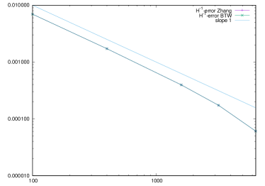
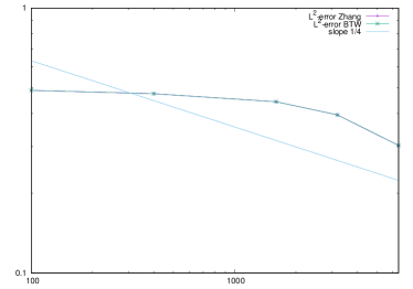
Figure 1: Experimental convergence of the error in the $H^{-1}$ norm for $M=100,400,1600,3200,6400$ at time $T=0.1$ for the Zhang and BTW model with $\sigma=0.03$ (left) and the corresponding error measured in the $L^{2}$ norm (right).

This improved convergence behavior for smaller mesh size can be explained by an interplay of the noise intensity with the dissipative effect of the diffusion: Since the variance of the noise scales with $\frac{1}{h}$, the smaller the mesh size, the larger the fluctuations of the noise. Since the diffusion is active only on supercritical sites ($|X_{h}|>K$) and absent on subcritical sites ($|X_{h}|<K$), the regularizing effect of the diffusion becomes more pronounced when the values of the solutions are driven towards larger values by an exploding variance of the noise.

This intuitive explanation suggests that an increase of the noise intensity $\sigma$ should lead to an improved convergence behavior in the $L^{2}$ norm. This motivates the following simulations: In Figure 2 we display the order of convergence for stronger noise $\sigma=0.17$, the results are again averaged over $100$ realizations of the noise. We observe a linear convergence rate in the $H^{-1}$ norm and a convergence rate of order $1/4$ in the $L^{2}$ norm.

Figure 2: Experimental convergence of the error in the $H^{-1}$ norm for $M=100,400,1600,3200,6400$ at time $T=0.1$ for the Zhang and BTW model with $\sigma=0.17$ (left) and the corresponding error measured in the $L^{2}$ norm (right).

In particular, the convergence of the $L^{2}$ norm improves over the one observed for $\sigma=0.03$, in the sense that the rate of convergence becomes visible also at coarser mesh sizes. This improved behavior is consistent with the above explanation of the improved convergence for smaller mesh sizes.

The numerical solution averaged over $100$ realizations of the noise at the final time $T=0.1$, with $M=100,400,1600,3200,6400,12800$ and $\sigma=0.03$, is displayed in Figure 3. The solutions of the Zhang and BTW models are graphically indistinguishable.

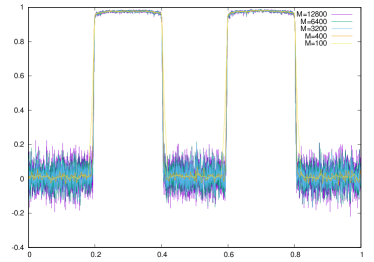
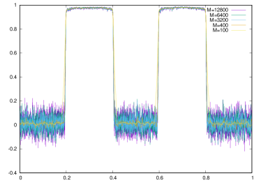
Figure 3: Numerical solution $X_{h}$ of the Zhang model (left) and the BTW model (right) at time $T=0.1$ for $\sigma=0.03$ averaged over $100$ realizations of the noise.

The numerical solutions averaged over $100$ realizations of the noise at the final time $T=0.1$, with $M=100,400,1600,3200,6400,12800$ and the stronger noise $\sigma=0.17$, is displayed in Figure 4. The simulations of the Zhang and BTW models are similar but there are noticeable differences in the regions where $X_{h}\approx K$ due to the different effects of the respective nonlinearities.

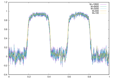
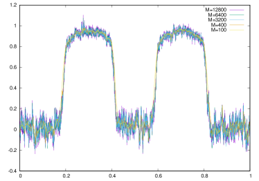
Figure 4: Numerical solution $X_{h}$ of the Zhang model (left) and the BTW model (right) at time $T=0.1$ for $\sigma=0.17$ averaged over $100$ realizations of the noise.

Numerical solutions of the Zhang model for a single realization of the noise for $\sigma=0.03,0.17$ are displayed in Figure 5. Again, we observe the improved ”smoothing” effect for stronger noise intensity $\sigma=0.17$.

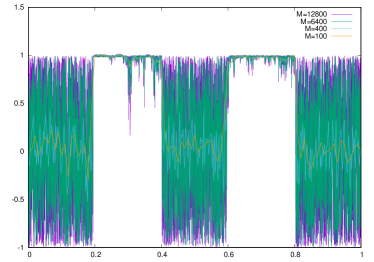
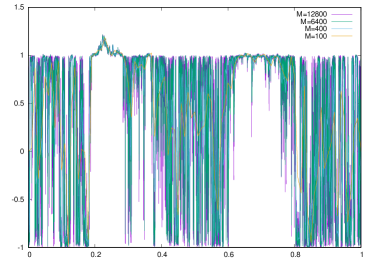
Figure 5: Single realization of the numerical solution $X_{h}$ of the Zhang model for $\sigma=0.03$ (left) and $\sigma=0.17$ (right) at time $T=0.1$ for different mesh size.

4.2 Power law scaling

A fundamental property of the original BTW model is the observation of power law scalings without explicit tuning of parameters to critical values, see [3]. In particular, it is observed that the size/duration of avalanches shows a power law scaling. In this section, we investigate the validity of such power law scalings for the weakly driven BTW/Zhang model (1.5) and their dependency on the grid size.

More precisely, we consider the discrete model (4.1) in spatial dimension $d=2$ and, if not mentioned otherwise, we set $K=10$, $D=0.25$ and $\mu=10^{-4}$, $\sigma=0.01$. The spatial domain is taken to be a unit square, that is covered by a uniform grid $z_{i,j}=(ih,jh)$ with mesh size $h=1/M$. The discrete two-dimensional Laplace operator is defined as

$$\Delta_{h}X(z_{i,j})=\frac{1}{h^{2}}\Big{(}-4X(z_{i,j})+X(z_{i-1,j})+X(z_{i+1,j})+X(z_{i,j-1})+X(z_{i,j+1})\Big{)}.$$

In all simulations below, the initial condition is chosen randomly and subcritical, that is, $\max_{j}|X_{h}^{0}(z_{j})|\leq K$. This is realized by sampling a random initial condition and subsequently simulating only the deterministic dynamics without forcing until a subcritical state is attained. This state is then taken as the initial condition for the subsequent simulations.

The duration and size of avalanches is defined as follows: Starting from a “subcritical” point in time $n_{0}\geq 0$, that is, $n_{0}$ such that all sites are subcritical in the sense that $\max_{j}|X_{h}^{n_{0}}(z_{j})|\leq K$, we say that an avalanche occurs at time point $n_{*}>n_{0}$ if $\max_{j}|X_{h}^{n}(z_{j})|\leq K$ for $n_{0}\leq n<n_{*}$ and $\max_{j}|X_{h}^{n_{*}}(z_{j})|>K$. The duration of this avalanche is then defined as the number of time-steps until the numerical solution reaches a subcritical level again, that is, until $\max_{j}|X^{n^{*}}_{h}(z_{j})|\leq K$ is reached for some $n^{*}>n_{*}$. The avalanche size is defined as $\#\{z_{j}:\ |X_{h}^{n}(z_{j})|>K\ \text{for some}\ n\in[n_{*},n^{*}]\}$.

Note that in dimension $d=2$ the existence and regularity of solutions of the SPDE (4.2), as well as the convergence of the numerical approximation (4.1) are open problems. Nevertheless, the numerical results reported in this section reveal power-law characteristics which appear to be preserved for decreasing mesh size.

Figure 6 displays log-scale plots of avalanche sizes and durations depending on different values of the parameters. We observe that, up to a certain threshold, the values of $\mu$ have a negligible effect on the statistics of the avalanches. Furthermore, we observe that the noise intensity $\sigma$ mainly influences the lower range of the size and duration of the avalanches, i. e. larger noise variance increases the frequency of smaller avalanches.

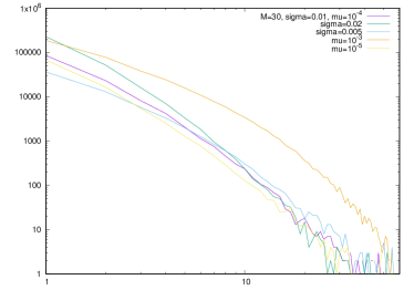
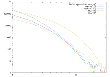
Figure 6: Log-scale plot of the frequency of avalanche sizes (left) and the duration of the avalanches (right).

Next, we examine the dependence of the avalanche statistics on the mesh size. In Figure 7 we display the log-scale plot of the avalanche size and duration for $M=15,30,60$. We observe that the power-law distributions for decreasing mesh size exhibit a similar shape.

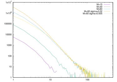
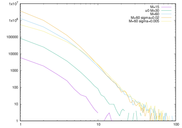
Figure 7: Log-scale plot of the the frequency of avalanche sizes (left) and the duration of the avalanches (right) for $M=15,30,60$.

We compare the scaling for the BTW model and the Zhang model in Figure 8. The scaling appears to be qualitatively similar with the difference that the frequency of smaller avalanches is higher in the BTW model.

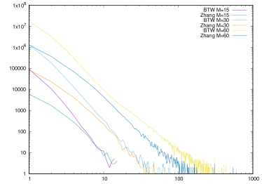
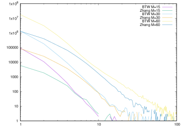
Figure 8: Log-scale plot of the the frequency of avalanche sizes (left) and the duration of the avalanches (right): comparison of BTW and Zhang models for $M=15,30,60$.

4.3 Scaling with totally asymmetric noise

The original BTW model introduced in [3] enforces a strict separation of time scales between the random forcing of the system and its relaxation into subcritical states by diffusion. This is realized by stopping the forcing during an avalanche until a subcritical state is reached. In addition, in [3] the noise is totally asymmetric, in the sense that energy is only added. In contrast, in the discrete model (4.1) both dynamics are active simultaneously, and energy is randomly added or subtracted, with positive average. The relative speed of driving by random forcing and diffusion can be steered by varying their relative intensities $D,\mu,\sigma$.

In this section, we compare the power-law scaling of the discrete model in two spatial dimensions with weakly asymmetric noise (i.e., noise also taking negative values) to the same model with a totally asymmetric noise instead (i.e., noise which only takes positive values). We consider the same parameters as in the previous section except for $\mu=0$, $\sigma=10^{-3}$ and the random variables $(\xi^{n,j}_{h})$ are chosen to have an i.i.d. Bernoulli distribution with values $\{0,1\}$ achieved with equal probability $\frac{1}{2}$.

In view of [3], we compare the avalanche statistics of simulations with strict scale separation to those with simultaneous forcing. In the first regime, the random forcing is switched off during an avalanche until the system reaches a subcritical state, while in the latter regime, the forcing remains active during avalanches.

In Figure 9 we display the the log-scale plots of avalanche sizes and durations. We observe that the avalanche distribution for the model with simultaneous forcing and diffusion and with larger mesh size $M=30$ and $\sigma=10^{-3}$ obeys a power law. For larger intensity of the asymmetric noise $\sigma=4\cdot 10^{-3}$ the power law is no longer preserved and the distribution is biased towards avalanches with larger size and duration. A similar situation occurs in the simulation with smaller mesh size $M=60$, $\sigma=10^{-3}$. In contrast, enforcing the strict scale separation of driving force and diffusion as in [3], the avalanche distribution obeys a power law even in the case $M=60$.

An explanation for these observations is that the effect of “overlapping avalanches” becomes dominant for large noise intensities: In systems near criticality, multiple simultaneous avalanches may occur, which, due to the global character of the avalanche definition, are counted as one large event. As a result, large avalanches would be overrepresented in the simulation. This effect is avoided when the strict separation of forcing and relaxation scale is enforced.

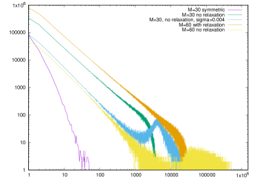
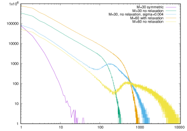
Figure 9: Log-scale plot of the frequency of avalanche sizes (left) and the duration of the avalanches (right) for asymmetric noise.

4.4 Simulations and scaling limits in 2D

In this section we investigate the existence of scaling limits of the discrete dynamics (4.1) in spatial dimension $d=2$, with a focus on the effect of the lower regularity of the limiting space-time white noise compared to one spatial dimension.

The simulation parameters are as follows: $T=0.015625$, $\sigma=1$, $\mu=0$, $D=0.25$, $K=1$, $\tau=h^{2}$, $h=1/128$, the spatial domain is the unit square $(0,1)^{2}$ and the initial condition is taken as $x_{h}^{0}=\frac{1}{2}\mathds{1}_{[0.25,0.75]\times[0.25,0.75]}$.

In Figure 11 we display the expected value of the discrete model (4.1) with Zhang nonlinearity at the final time $T$ averaged over $10^{6}$ realizations and with mesh size $h=1/128$. The analogous expected value of (4.1) with BTW nonlinearity is displayed in Figure 12 (left). For better comparison the color range is restricted to $[0,0.5]$. There are only minor overshoots of these values due to the error of the Monte-Carlo approximation of the expected value in the stochastic case. In Figure 11 (right), for comparison, we display the expected value of (4.1) with $\phi(x)=x$ corresponding to the stochastic heat equation

We observe that the simulation of (4.1) with Zhang nonlinearity is very similar to the expectation of the numerical solution of the stochastic heat equation (i.e., the linear counterpart of (4.1)). In contrast, the simulation of (4.1) with BTW nonlinearity is closer to the initial condition, that is, the effect of the diffusion is weaker in this case.

To offer an explanation of this observation, we note that the computed probability of the solution to be supercritical, i.e., $\frac{\mathbb{E}\left[\#\{z_{i,j}:\,\,|X_{h}^{n}(z_{i,j})|\geq K\}\right]}{\#\{z_{i,j}\}}$ (not counting the grid points at the boundary) is above $0.50$, and the probability increases with smaller mesh size due to the scaling of the noise with $h^{-1}$, see Figure 10 where we display the computed evolution of the probability for the Zhang model. Since in the supercritical “regime”, the effect of the diffusion of the Zhang nonlinearity is identical to that of the stochastic heat equation, this could offer an explanation of the observation above. In contrast, the BTW nonlinearity does not equal that of the heat equation even for supercritical values of the solution. Therefore, one expects that, even for small grid size $h$, the BTW model behaves differently from the stochastic heat equation, which is indeed observed in Figure 12.

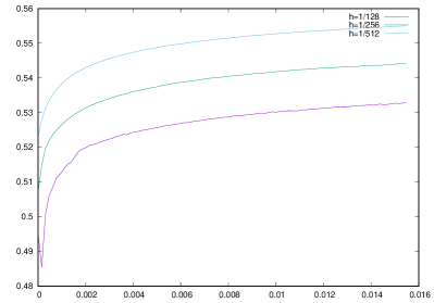
Figure 10: Evolution of $\frac{\mathbb{E}\left[\#\{z_{i,j}:\,\,|X_{h}^{n}(z_{i,j})|\geq K\}\right]}{\#\{z_{i,j}\}}$ for $h=1/128,1/256,1/512$ for the Zhang model.

To illustrate the effect of the fluctuations and the resulting irregularity of the solution we display one realization of the solution of the BTW model at the final time in Figure 12 (right). In contrast to the 1d case (see Figures 3 and 4) the solution oscillates and exceeds the critical value $K$.

We note that in the deterministic case, for the considered parameters, the solutions of the Zhang and BTW model are equal to the initial condition since $\max_{i,j}|X^{0}_{h}(z_{i,j})|\leq\frac{1}{2}<K$.

Repeating the simulations with the initial condition taken to be the (unscaled) indicator function of a square with side $\frac{1}{2}$ placed at the center of the domain yielded analogous results (not displayed).

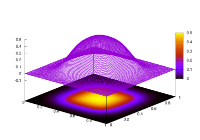
Figure 11: Expected value of the numerical solution computed with the Zhang model (left) and the stochastic heat equation (right) at time $t=T$.

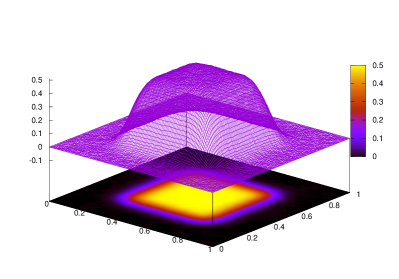
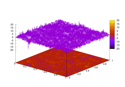
Figure 12: Expected value of the numerical solution computed with the BTW model (left) and one realization of the solution of the BTW model (right) at time $t=T$.

Appendix A Uniqueness of laws of weak solutions

In this section, we prove the following, using the main result from [63].

Theorem A.1.

The processes $(\tilde{X},\tilde{W})$ of every weak solution to (2.2) have the same law with respect to the Borel $\sigma$-algebra of $L^{2}([0,T];L^{2})\times\mathcal{C}([0,T];{H^{-1}})$.

We first give some preparatory results and helpful notions.

Definition A.2.

We define a multivalued operator by its graph $\mathcal{A}_{T}\subset L^{2}([0,T];L^{2})\times L^{2}([0,T];L^{2})$, given by

$$(f,g)\in\mathcal{A}_{T}\quad\text{if and only if}\quad g\in\phi_{2}(f)\ \text{for almost every }(t,x)\in[0,T]\times[0,1].$$ (A.1)

Lemma A.3.

The operator $\mathcal{A}_{T}$ is maximal monotone.

Proof.

By [4, Theorem 2.8], it is enough to show that $\mathcal{A}_{T}$ is the subdifferential of a convex, proper and lower-semicontinuous functional $\varphi:H\to[0,\infty]$ on a real Banach space $H$. To this end, define $\tilde{\psi}:\mathbb{R}\to[0,\infty)$ by

$$\tilde{\psi}(x)=\mathds{1}_{\{\left|x\right|\geq 1\}}(x^{2}-1),$$

which is proper, convex and continuous, and for which we have $\partial\tilde{\psi}=\phi_{2}$. We note that $H:=L^{2}([0,T];L^{2})$ is a Hilbert space. Defining

$$\varphi_{T}:H\to[0,\infty],\quad\varphi_{T}(u)=\int_{0}^{T}\int_{0}^{1}\tilde{\psi}(u(t,x))\mathrm{d}x\mathrm{d}t,$$ (A.2)

we obtain by [18, Theorem 16.50] that $\varphi_{T}$ is convex, proper and lower-semicontinuous and $\mathcal{A}_{T}=\partial\varphi_{T}$, as required. ∎

Lemma A.4.

The graph $\mathcal{A}_{T}$ is a closed subset of $L^{2}([0,T];L^{2})\times L^{2}([0,T];L^{2})$ and thus measurable with respect to the Borel $\sigma$-algebra on $L^{2}([0,T];L^{2})$.

Proof.

The first statement is true for any maximal monotone operator by [4, Proposition 2.1]. The measurability then follows by definition of the Borel $\sigma$-algebra. ∎

We define two kinds of Sobolev spaces that we are going to use.

Definition A.5.

Let $V\subset H\subset V^{\prime}$ a Gelfand triple and $T>0$. We define

$$W^{1,2}([0,T];V^{\prime}) :=\{u\in L^{2}([0,T];V^{\prime}):u^{\prime}\in L^{2}([0,T];V^{\prime})\}$$

$$\text{and}\quad W^{1,2}([0,T];V,H) :=\{u\in L^{2}([0,T],V):u^{\prime}\in L^{2}([0,T];V^{\prime})\},$$

where $u^{\prime}$ is the weak derivative of $u$ as defined e. g. in [59, Definition 2.5.1]. These spaces are Banach spaces with the norms

$$\left\lVert u\right\rVert_{W^{1,2}([0,T];V^{\prime})} =\left(\left\lVert u\right\rVert_{L^{2}([0,T];V^{\prime})}^{2}+\left\lVert u^{\prime}\right\rVert_{L^{2}([0,T];V^{\prime})}^{2}\right)^{\frac{1}{2}}$$

$$\text{and}\quad\left\lVert u\right\rVert_{W^{1,2}([0,T];V,H)} =\left(\left\lVert u\right\rVert_{L^{2}([0,T];V)}^{2}+\left\lVert u^{\prime}\right\rVert_{L^{2}([0,T];V^{\prime})}^{2}\right)^{\frac{1}{2}},$$

respectively. These norms are norm-equivalent to the ones given in [59, Section 2.5.b] and [86, Proposition 23.23], respectively, where also the Banach space property is proved.

We have the following measurability properties.

Lemma A.6.

The subset

$$M_{1}:=\left\{\begin{aligned} &\qquad\qquad\qquad\quad(u,z)\in L^{2}([0,T];L^{2})\times L^{2}([0,T];(L^{2})^{\prime}):\\ &\exists v\in L^{2}([0,T];L^{2})\text{ such that }z=\Delta v\ \mathrm{d}t\text{-almost everywhere and }(u,v)\in\mathcal{A}_{T}\end{aligned}\right\}$$ (A.3)

is Borel-measurable. The map $\partial_{t}:W^{1,2}([0,T];(L^{2})^{\prime})\to L^{2}([0,T];(L^{2})^{\prime})$ is continuous and

$$M_{2}:=(\Pi_{1},\partial_{t}(\Pi_{2}))^{-1}(M_{1})\subseteq L^{2}([0,T];L^{2})\times W^{1,2}([0,T];(L^{2})^{\prime})$$ (A.4)

is Borel-measurable. The set $M_{2}$ is also Borel-measurable as a subset of $L^{2}([0,T];L^{2})\times L^{2}([0,T];(L^{2})^{\prime})$. Finally, let $I_{xw}:L^{2}([0,T];L^{2})\times\mathcal{C}([0,T];{H^{-1}})\hookrightarrow\left(L^{2}([0,T];(L^{2})^{\prime})\right)^{2}$ be the canonical continuous embedding. Then, the subset

$$M_{3}:=\left\{\left(\Pi_{1},\Pi_{1}(I_{xw})-\Pi_{2}(I_{xw})\right)-\mu t\in M_{2}\right\}\subseteq L^{2}([0,T];L^{2})\times\mathcal{C}([0,T];{H^{-1}})$$

is Borel-measurable, where we write $\mu t\in L^{2}([0,T];(L^{2})^{\prime})$ for the canonically embedded $L^{2}([0,T];L^{2})$ function given by

$$(t,x)\mapsto\mu t.$$

Proof.

We notice that $M_{1}$ is the image of the set $\mathcal{A}_{T}$, which is Borel-measurable by Lemma A.4, under the isometry $(\Pi_{1},\Delta\circ\Pi_{2})$, and hence Borel-measurable by the Kuratowski theorem (cf. [73, Theorem 3.9]). The operator $\partial_{t}:W^{1,2}([0,T];(L^{2})^{\prime})\to L^{2}([0,T];(L^{2})^{\prime})$ is linear and bounded by the definition of the Sobolev space. Hence it is continuous, which implies Borel-measurability. Thus, also $(\Pi_{1},\partial_{t})$ is continuous and Borel-measurable, which yields measurability of $M_{2}$ using the measurability of $M_{1}$. The set $M_{2}$, viewed as a subset of $L^{2}([0,T];L^{2})\times L^{2}([0,T];(L^{2})^{\prime})$, is the image of the canonical embedding and thus Borel-measurable by the Kuratowski theorem. The Borel-measurability of $M_{3}$ follows by the continuity of $I_{xw}$. ∎

The previous lemma alludes that (2.3) and (2.4) are actually distributional properties, which motivates the following definition.

Definition A.7.

We call a probability measure $Q$ on the probability space $L^{2}([0,T];L^{2})\times\mathcal{C}([0,T];{H^{-1}})$ endowed with its Borel $\sigma$-algebra a pre-solution to (2.2), if

$$Q(M_{3})=1,$$ (A.5)

where $M_{3}$ is defined as in Lemma A.6.

Lemma A.8.

The joint law of the processes $(X,W)$ of each weak solution to (2.2) in the sense of Definition 2.1 is a pre-solution.

Proof.

Let $\left((\Omega,\mathcal{F},(\mathcal{F}_{t})_{t\in[0,T]},\mathbb{P}),X,W\right)$ be a weak solution to (2.2) and $Y\in L^{2}(\tilde{\Omega}\times[0,T];L^{2})$ the corresponding drift process as in Definition 2.1. Then, [59, Proposition 2.5.9], (2.3) and (2.4) yield

$$\partial_{t}\left(\Pi_{1}(I_{xw}(X,W))-\Pi_{2}(I_{xw}(X,W))-\mu t\right)=\Delta Y\quad\mathbb{P}\text{-almost surely}$$

with $(X,Y)\in\mathcal{A}_{T}$. Hence, using the notation from Lemma A.6, we have

$$\left(X,\partial_{t}(\Pi_{1}(I_{xw}(X,W))-\Pi_{2}(I_{xw}(X,W))-\mu t)\right)\in M_{1}\quad\mathbb{P}\text{-almost surely},$$

which by construction is equivalent to $(X,W)\in M_{3}$ $\mathbb{P}$-almost surely. This finishes the proof. ∎

We cite the concept of pointwise uniqueness from [63, Definition 1.4].

Definition A.9.

Pointwise uniqueness holds for pre-solutions, if and only if for any processes $(X_{1},X_{2},W)$ defined on the same probability space with $\mathcal{L}((X_{1},W))$ and $\mathcal{L}((X_{2},W))$ being pre-solutions, $X_{1}=X_{2}$ almost surely.

Lemma A.10.

Pointwise uniqueness holds for pre-solutions to (2.2).

Proof.

Let $(X^{1},X^{2},W)$ be defined on a probability space $(\Omega,\mathcal{F},\mathbb{P})$, such that $\mathcal{L}((X^{1},W))$ and $\mathcal{L}((X^{2},W))$ are two pre-solutions to (2.2). Let $M_{3}$ be defined as in Lemma A.6, and let

$$\tilde{M}_{3}:=(X^{1},W)^{-1}(M_{3})\cap(X^{2},W)^{-1}(M_{3}),$$

which implies that $\mathbb{P}(\tilde{M}_{3})=1$ by construction. From now on, we conduct all arguments pointwise for $\omega\in\tilde{M}_{3}$. We define $Y^{i}\in L^{2}([0,T];L^{2})$ for $i=1,2$ by

$$Y^{i}=\Delta^{-1}(\partial_{t}(X^{i}-W-\mu t)),$$

which is well-defined due to the construction of $M_{3}$. Moreover, it follows that (2.3) and (2.4) are satisfied for $(X^{i},Y^{i},W)$ for $i=1,2$, which implies

$$X^{1}(t)-X^{2}(t)=\int_{0}^{t}\Delta(Y^{1}(r)-Y^{2}(r))\mathrm{d}r\quad\text{in }L^{2}([0,T];(L^{2})^{\prime}).$$ (A.6)

By [59, Proposition 2.5.9], (A.6) implies that $X^{1}-X^{2}$ is weakly differentiable with $(X^{1}-X^{2})^{\prime}=\Delta(Y^{1}-Y^{2})$. Since $X^{i},Y^{i}\in L^{2}([0,T];L^{2})$ for $i=1,2$ by construction, $X^{1}-X^{2}\in W^{1,2}([0,T];L^{2},{H^{-1}})$. [86, Proposition 23.23] then yields that there exists a continuous ${H^{-1}}$-valued $\mathrm{d}t$-version $Z$ of $X^{1}-X^{2}$, for which we have

$$\left\lVert Z(t)\right\rVert_{H^{-1}}^{2} =\int_{0}^{t}\left\langle\Delta(Y^{1}(r)-Y^{2}(r)),X^{1}(r)-X^{2}(r)\right\rangle_{(L^{2})^{\prime}\times L^{2}}\mathrm{d}r$$

$$=-\int_{0}^{t}\left\langle Y^{1}(r)-Y^{2}(r),X^{1}(r)-X^{2}(r)\right\rangle_{L^{2}}\mathrm{d}r\leq 0,$$

where the last step follows from (2.4). This implies that $Z$ and consequently $X^{1}-X^{2}$ is zero $\mathrm{d}t$-almost everywhere. Since this is true for every $\omega\in\tilde{M}_{3}$, $X^{1}=X^{2}$ $\mathbb{P}$-almost surely, as required. ∎

Corollary A.11.

There exists at most one pre-solution to (2.2).

Proof.

This is part of the statement of [63, Theorem 1.5]. ∎

Proof of Theorem A.1.

The claim is a direct consequence of Lemma A.8 and Corollary A.11. ∎

Appendix B Properties of discrete spaces and prolongations

We state some properties on the discrete spaces used above and their interplay to the corresponding function spaces by via prolongations. For the sake of brevity, we omit details which can be considered classical.

Lemma B.1.

Let $\Delta_{h}\in\mathbb{R}^{(Z-1)\times(Z-1)}$ be defined as in (1.11). Then, $-\Delta_{h}$ is positive definite and

$$\left\lVert-\Delta_{h}\right\rVert\leq\frac{4}{h^{2}}.$$

Proof.

From [64, Equation (2.23)], we obtain that the eigenvalues of $-\Delta_{h}$ are

$$\lambda_{j}=\frac{2}{h^{2}}(1-\cos(j\pi h))\in\left(0,\frac{4}{h^{2}}\right),\quad j=1,\dots,Z-1,$$

which implies that $-\Delta_{h}$ is positive definite. Equation (2.77) in [82] then yields the second claim. ∎

Corollary B.2.

For $u\in\mathbb{R}^{Z-1}$, Lemma B.1 yields

$$\begin{split}\left\lVert\Delta_{h}u\right\rVert_{-1}^{2}&=\left|\left\langle-\Delta_{h}u,u\right\rangle_{0}\right|=h\left|\left\langle-\Delta_{h}u,u\right\rangle\right|\\ &\leq h\left\lVert-\Delta_{h}u\right\rVert\left\lVert u\right\rVert\leq\left\lVert-\Delta_{h}\right\rVert h\left\lVert u\right\rVert^{2}\leq\frac{4}{h^{2}}\left\lVert u\right\rVert_{0}^{2}.\end{split}$$ (B.1)

Lemma B.3.

Let $h>0$ as in Assumption 2.2, and let $I^{\prime}:L^{2}\to{H^{-1}}$ be the canonical embedding. Then, $I^{\prime}\in L_{2}(L^{2},{H^{-1}})$ and

$$\lim_{h\to 0}\mathrm{Tr}(-\Delta_{h}^{-1})=\sum_{k=1}^{\infty}\frac{1}{\pi^{2}k^{2}}=\frac{1}{6}=\left\lVert I^{\prime}\right\rVert_{L_{2}(L^{2},{H^{-1}})}^{2}.$$ (B.2)

Recall the partitions $(K_{i})_{i=0}^{Z}$ and $(J_{i})_{i=0}^{Z-1}$ and the grids $(x_{i})_{i=0}^{Z}$ and $(y_{i})_{i=0}^{Z-1}$ as given in (1.10), and the definition of prolongations of functions on these grids as given in Definition 1.5 and Definition 1.8. Then, the following statements can be verified by direct computations.

Lemma B.4.

Let $u=(u_{i})_{i=1}^{Z-1}\in\mathbb{R}^{Z-1}$ and $v=(v_{i})_{i=0}^{Z-1}\in\mathbb{R}^{Z}$ and recall the convention $u_{0}=u_{Z}=0$. Define the piecewise linear prolongation with zero-Neumann boundary conditions with respect to the grid $(y_{i})_{i=0,\dots,Z-1}$ by

$$I_{h}^{\mathrm{ply}}\,:\mathbb{R}^{Z}\to H^{1},v\mapsto v_{0}\mathds{1}_{K_{0}}+\sum_{i=1}^{Z-1}\left[v_{i-1}+\frac{v_{i}-v_{i-1}}{h}(\cdot-x_{i})\right]\mathds{1}_{K_{i}}+v_{Z-1}\mathds{1}_{K_{Z}}.$$

and the piecewise constant prolongation by $I_{h}^{\mathrm{pcy}}\,:\mathbb{R}^{Z}\to L^{2},v\mapsto\sum_{i=0}^{Z-1}v_{i}\mathds{1}_{J_{i}}$. Then,

$$\left\lVert I_{h}^{\mathrm{ply}}\,v\right\rVert_{L^{2}}\leq\left\lVert I_{h}^{\mathrm{pcy}}\,v\right\rVert_{L^{2}}\leq 3\left\lVert I_{h}^{\mathrm{ply}}\,v\right\rVert_{L^{2}},$$

$$\int_{0}^{1}I_{h}^{\mathrm{ply}}\,v\ \mathrm{d}x=\int_{0}^{1}I_{h}^{\mathrm{pcy}}\,v\ \mathrm{d}x,$$

$$I_{h}^{\mathrm{ply}}\,v-a=I_{h}^{\mathrm{ply}}\,(v-a)\quad\text{and}\quad I_{h}^{\mathrm{pcy}}\,v-a=I_{h}^{\mathrm{pcy}}\,(v-a)\quad\text{for all }a\in\mathbb{R},$$

$$\partial_{x}I_{h}^{\mathrm{pcy}}\,v=\sum_{i=1}^{Z-1}\delta_{x_{i}}(v_{i}-v_{i-1}),$$

$$\partial_{x}\left(I_{h}^{\mathrm{ply}}\,\left(\sum_{j=0}^{i}hu_{j}\right)_{i=0}^{Z-1}\right)=I_{h}^{\mathrm{pcx}}\,u,$$

$$\left\lVert u\right\rVert_{1}=\left\lVert I_{h}^{\mathrm{plx}}\,u\right\rVert_{H^{1}_{0}},$$

$$\left\lVert\partial_{xx}(I_{h}^{\mathrm{plx}}\,u)\right\rVert_{H^{-1}}=\left\lVert\sum_{i=1}^{Z-1}\frac{1}{h}(-u_{i-1}+2u_{i}-u_{i+1})\delta_{x_{i}}\right\rVert_{H^{-1}}.$$

Lemma B.5.

Let $u=(u_{i})_{i=1}^{Z-1}\in\mathbb{R}^{Z-1}$, where $Z$ is defined as in (1.10). Then

$$\left\lVert I_{h}^{\mathrm{pcx}}\,u\right\rVert_{H^{-1}}\leq\left\lVert u\right\rVert_{-1}\leq 3\left\lVert I_{h}^{\mathrm{pcx}}\,u\right\rVert_{H^{-1}}.$$

Proof.

Let $v=(v_{i})_{i=0}^{Z-1}\in\mathbb{R}^{Z}$ be defined by $v_{i}=\sum_{j=0}^{i}hu_{j}$. Then, using the convention $\left(\Delta_{h}^{-1}u\right)_{0}=\left(\Delta_{h}^{-1}u\right)_{Z}=0$ and Lemma B.4, we have

$$\left\lVert I_{h}^{\mathrm{pcx}}\,u\right\rVert_{H^{-1}}=\left\lVert I_{h}^{\mathrm{ply}}\,v-\int_{0}^{1}I_{h}^{\mathrm{ply}}\,v\ \mathrm{d}x\right\rVert_{L^{2}}=\left\lVert I_{h}^{\mathrm{ply}}\,\left(v-\int_{0}^{1}I_{h}^{\mathrm{ply}}\,v\ \mathrm{d}x\right)\right\rVert_{L^{2}}$$

$$\leq\left\lVert I_{h}^{\mathrm{pcy}}\,\left(v-\int_{0}^{1}I_{h}^{\mathrm{pcy}}\,v\ \mathrm{d}x\right)\right\rVert_{L^{2}}=\left\lVert\partial_{x}(I_{h}^{\mathrm{pcy}}\,v)\right\rVert_{H^{-1}}=\left\lVert\sum_{i=1}^{Z-1}\delta_{x_{i}}hu_{i}\right\rVert_{H^{-1}}$$

$$=\left\lVert\sum_{i=1}^{Z-1}\delta_{x_{i}}h(\Delta_{h}\Delta_{h}^{-1}u)_{i}\right\rVert_{H^{-1}}=\left\lVert\sum_{i=1}^{Z-1}\delta_{x_{i}}\frac{1}{h}\left(-\left(\Delta_{h}^{-1}u\right)_{i-1}+2\left(\Delta_{h}^{-1}u\right)_{i}-\left(\Delta_{h}^{-1}u\right)_{i+1}\right)\right\rVert_{H^{-1}}$$

$$=\left\lVert\partial_{xx}(I_{h}^{\mathrm{plx}}\,\Delta_{h}^{-1}u)\right\rVert_{H^{-1}}=\left\lVert I_{h}^{\mathrm{plx}}\,\Delta_{h}^{-1}u\right\rVert_{H^{1}_{0}}=\left\lVert\Delta_{h}^{-1}u\right\rVert_{1}=\left\lVert u\right\rVert_{-1},$$

which yields the first inequality. The same calculation yields the second inequality if we start with $3\left\lVert I_{h}^{\mathrm{pcx}}\,u\right\rVert_{H^{-1}}$ and replace the third step by

$$3\left\lVert I_{h}^{\mathrm{ply}}\,\left(v-\int_{0}^{1}I_{h}^{\mathrm{ply}}\,v\ \mathrm{d}x\right)\right\rVert_{L^{2}}\geq\left\lVert I_{h}^{\mathrm{pcy}}\,\left(v-\int_{0}^{1}I_{h}^{\mathrm{pcy}}\,v\ \mathrm{d}x\right)\right\rVert_{L^{2}}.$$

∎

Proposition B.6.

Let $h>0$ denote a sequence converging to $0$, $u\in L^{2}([0,T];{H^{-1}})$, $\eta\in L^{2}([0,T];L^{2})$, and for all $h$ in this sequence, $t\in[0,T]$, let $u_{h}(t),\eta_{h}(t)\in\mathbb{R}^{Z-1}$ such that ${u_{h}^{\text{pcx}}}\in L^{2}([0,T];{H^{-1}})$ with ${u_{h}^{\text{pcx}}}\rightharpoonup u$ in $L^{2}([0,T];{H^{-1}})$ and ${\eta_{h}^{\text{pcx}}}\in L^{2}([0,T];L^{2})$ with ${\eta_{h}^{\text{pcx}}}\to\eta$ in $L^{2}([0,T];L^{2})$. Then, for $h\to 0$,

$$\int_{0}^{T}\left\langle\eta_{h}(t),u_{h}(t)\right\rangle_{-1}\mathrm{d}t\to\int_{0}^{T}\left\langle\eta(t),u(t)\right\rangle_{H^{-1}}\mathrm{d}t.$$

Proof.

After deriving a Poincaré inequality for the discrete norms, i. e. $\left\lVert v\right\rVert_{0}^{2}\leq C\left\lVert v\right\rVert_{1}^{2}$ for $v\in\mathbb{R}^{Z-1}$, the uniform bound of ${u_{h}^{\text{pcx}}}$ in $L^{2}([0,T];{H^{-1}})$ implies a uniform bound of ${(-\Delta_{h}^{-1}u_{h})^{\text{pcx}}}$ in $L^{2}([0,T];L^{2})$. This allows to extract a weakly converging nonrelabeled subsequence with limit $f\in L^{2}([0,T];L^{2})$. In order to show that $f=-\Delta u$, it is key to realize that

$$\xi(t,x){\left(-\Delta_{h}u_{h}(t)\right)^{\text{pcx}}}(x)=-\xi(t,x)\left(D_{h}^{-}D_{h}^{+}{u_{h}^{\text{pcx}}}(t)\right)(x)\quad\text{for almost all }t\in[0,T],x\in[0,1]$$ (B.3)

for a test function $\xi\in\mathcal{C}_{c}^{\infty}([0,T]\times[0,1])$, where $D_{h}^{\pm}$ are the $h$-difference quotients to the left resp. right. Hence, conducting a discrete integration by parts and considering that $\xi$ has compact support, we compute

$$\begin{split}&\int_{0}^{T}\left\langle u,\xi\right\rangle_{{H^{-1}}\times{H^{1}_{0}}}\mathrm{d}t=\lim_{h\to 0}\int_{0}^{T}\left\langle{\bar{u}_{h}^{\text{pcx}}},\xi\right\rangle_{L^{2}}\mathrm{d}t=\lim_{h\to 0}\int_{0}^{T}\left\langle{\left(\Delta_{h}\Delta_{h}^{-1}u_{h}\right)^{\text{pcx}}},\ \xi\right\rangle_{L^{2}}\mathrm{d}t\\ &=\lim_{h\to 0}\int_{0}^{T}\left\langle-D_{h}^{-}D_{h}^{+}{\left(-\Delta_{h}^{-1}u_{h}\right)^{\text{pcx}}},\ \xi\right\rangle_{L^{2}}\mathrm{d}t\\ &=\lim_{h\to 0}\int_{0}^{T}\left\langle{\left(-\Delta_{h}^{-1}u_{h}\right)^{\text{pcx}}},-D_{h}^{-}D_{h}^{+}\xi\right\rangle_{L^{2}}\mathrm{d}t=\int_{0}^{T}\left\langle f,-\Delta\xi\right\rangle_{L^{2}}\mathrm{d}t,\end{split}$$ (B.4)

using the strong convergence of the second-order difference quotient of $\xi$ to its second derivative. By a density argument, one concludes that $f=-\Delta u$ $\mathrm{d}t$-almost everywhere. The proof can then be finished by computing

$$\int_{0}^{T}\left\langle u_{h},\eta_{h}\right\rangle_{-1}\mathrm{d}t =\int_{0}^{T}\left\langle-\Delta_{h}^{-1}u_{h},\eta_{h}\right\rangle_{0}\mathrm{d}t=\int_{0}^{T}\left\langle{\left(-\Delta_{h}^{-1}u_{h}\right)^{\text{pcx}}},{\eta_{h}^{\text{pcx}}}\right\rangle_{L^{2}}\mathrm{d}t$$

$$\quad\to\int_{0}^{T}\left\langle-\Delta^{-1}u,\eta\right\rangle_{L^{2}}\mathrm{d}t=\int_{0}^{T}\left\langle u,\eta\right\rangle_{H^{-1}}\mathrm{d}t.$$

∎

Lemma B.7.

Recall Definitions 1.5 and 1.6 and let $u\in\mathbb{R}^{Z-1}$. Then there exists a constant $C$ independent of $h$ such that

$$\left\lVert u\right\rVert_{-1}^{2}\leq C\left\lVert u\right\rVert_{0}^{2}.$$

Proof.

Note that since $-\Delta_{h}$ is symmetric and positive definite, one may define its symmetric and positive definite sqare root operator $A_{h}$, which satisfies $A_{h}A_{h}=-\Delta_{h}$, $\left\lVert u\right\rVert_{1}=\left\lVert A_{h}u\right\rVert_{0}$ and $\left\lVert u\right\rVert_{-1}=\left\lVert A_{h}^{-1}u\right\rVert_{0}$. Furthermore, we have a Poincaré inequality for the discrete norms by

$$\left\lVert u_{h}\right\rVert_{0}^{2}=\left\lVert{u_{h}^{\text{pcx}}}\right\rVert_{L^{2}}^{2}\leq C\left\lVert{u_{h}^{\text{plx}}}\right\rVert_{L^{2}}^{2}\leq C\left\lVert\nabla{u_{h}^{\text{plx}}}\right\rVert_{L^{2}}^{2}=C\left\lVert u_{h}\right\rVert_{1}^{2}$$ (B.5)

for $C$ independent of $h$, where the first inequality can be obtained by connecting [41, Propositions 3.1 and 3.2], and the last equality is the sixth statement in Lemma B.4. We then compute

$$\left\lVert u\right\rVert_{-1}^{2}=\left\lVert A_{h}A_{h}^{-1}u\right\rVert_{-1}^{2}=\left\lVert A_{h}^{-1}u\right\rVert_{0}^{2}\leq C\left\lVert u\right\rVert_{0}^{2}.$$

∎

References

- [1] P. Bak. How nature works. Springer New York, 1996.
- [2] P. Bak, C. Tang, and K. Wiesenfeld. Self-organized criticality: An explanation of the 1/f noise. Phys. Rev. Lett., 59:381–384, 1987.
- [3] P. Bak, C. Tang, and K. Wiesenfeld. Self-organized criticality. Phys. Rev. A, 38:364–374, 1988.
- [4] V. Barbu. Nonlinear Differential Equations of Monotone Types in Banach Spaces. Springer New York, 2010.
- [5] V. Barbu. Self-organized criticality and convergence to equilibrium of solutions to nonlinear diffusion equations. Annual Reviews in Control, 34(1):52–61, 2010.
- [6] V. Barbu. Self-organized criticality of cellular automata model; absorbtion in finite-time of supercritical region into the critical one. Mathematical Methods in the Applied Sciences, 36(13):1726–1733, 2013.
- [7] V. Barbu. The steepest descent algorithm in wasserstein metric for the sandpile model of self-organized criticality. SIAM Journal on Control and Optimization, 55(1):413–428, 2017.
- [8] V. Barbu, P. Blanchard, G. Da Prato, and M. Röckner. Self-organized criticality via stochastic partial differential equations. Theta Series in Advanced Mathematics, "Potential Theory and Stochastic Analysis" in Albac. Aurel Cornea Memorial Volume, pages 11–19, 2009.
- [9] V. Barbu, V. I. Bogachev, G. Da Prato, and M. Röckner. Weak solutions to the stochastic porous media equation via Kolmogorov equations: The degenerate case. Journal of Functional Analysis, 237(1):54–75, 2006.
- [10] V. Barbu, G. Da Prato, and M. Röckner. Stochastic porous media equations and self-organized criticality. Communications in Mathematical Physics, 285(3):901–923, Feb 2009.
- [11] V. Barbu, G. Da Prato, and M. Röckner. Stochastic Porous Media Equations. Lecture Notes in Mathematics. Springer International Publishing, 2016.
- [12] V. Barbu, G. Da Prato, and M. Röckner. Existence of strong solutions for stochastic porous media equation under general monotonicity conditions. The Annals of Probability, 37(2):428–452, 2009.
- [13] V. Barbu, G. Da Prato, and M. Röckner. Finite time extinction of solutions to fast diffusion equations driven by linear multiplicative noise. Journal of Mathematical Analysis and Applications, 389(1):147 – 164, 2012.
- [14] V. Barbu and C. Marinelli. Strong solutions for stochastic porous media equations with jumps. Infinite Dimensional Analysis, Quantum Probability and Related Topics, 12(03):413–426, 2009.
- [15] V. Barbu, G. D. Prato, and M. Röckner. Existence and uniqueness of nonnegative solutions to the stochastic porous media equation. Indiana University Mathematics Journal, 57(1):187–211, 2008.
- [16] V. Barbu and M. Röckner. Stochastic porous media equations and self-organized criticality: Convergence to the critical state in all dimensions. Communications in Mathematical Physics, 311(2):539–555, Apr 2012.
- [17] V. Barbu, M. Röckner, and F. Russo. Stochastic porous media equations in . Journal de Mathématiques Pures et Appliquées, 103(4):1024–1052, 2015.
- [18] H. Bauschke and P. Combettes. Convex Analysis and Monotone Operator Theory in Hilbert Spaces. CMS Books in Mathematics. Springer International Publishing, 2017.
- [19] v. Baňas, B. Gess, and C. Vieth. Numerical approximation of singular-degenerate parabolic stochastic pdes, 2022. https://arxiv.org/abs/2012.12150.
- [20] J. Bouchaud, M. Cates, J. R. Prakash, and S. Edwards. A model for the dynamics of sandpile surfaces. Journal De Physique I, 4:1383–1410, 1994.
- [21] D. Breit, E. Feireisl, and M. Hofmanová. Incompressible limit for compressible fluids with stochastic forcing. Arch. Ration. Mech. Anal., 222(2):895–926, 2016.
- [22] P. Bántay and I. M. Jánosi. Self-organization and anomalous diffusion. Physica A, 185:11–18, 1992.
- [23] R. Cafiero, V. Loreto, L. Pietronero, A. Vespignani, and S. Zapperi. Local rigidity and self-organized criticality for avalanches. Europhysics Letters (EPL), 29(2):111–116, jan 1995.
- [24] J. M. Carlson, J. T. Chayes, E. R. Grannan, and G. H. Swindle. Self-organized criticality in sandpiles: nature of the critical phenomenon. Phys. Rev. A (3), 42(4):2467–2470, 1990.
- [25] J. M. Carlson, E. R. Grannan, G. H. Swindle, and J. Tour. Singular diffusion limits of a class of reversible self-organizing particle systems. Ann. Probab., 21(3):1372–1393, 1993.
- [26] P. Clément. An introduction to gradient flows in metric spaces, 2009. http://www.math.leidenuniv.nl/reports/files/2009-09.pdf, 16 April 2021.
- [27] G. Da Prato and M. Röckner. Weak solutions to stochastic porous media equations. Journal of Evolution Equations, 4(2):249–271, May 2004.
- [28] G. Da Prato, M. Röckner, B. L. Rozovskii, and F.-Y. Wang. Strong solutions of stochastic generalized porous media equations: Existence, uniqueness, and ergodicity. Communications in Partial Differential Equations, 31(2):277–291, 2006.
- [29] K. Dareiotis, B. Gess, M. V. Gnann, and G. Grün. Non-negative martingale solutions to the stochastic thin-film equation with nonlinear gradient noise, 2020.
- [30] B. Davis. On the integrability of the martingale square function. Israel J. Math., 8:187–190, 1970.
- [31] F. del Teso. Finite difference method for a fractional porous medium equation. Calcolo, 51(4):615–638, 2014.
- [32] F. del Teso, J. Endal, and E. R. Jakobsen. Robust numerical methods for nonlocal (and local) equations of porous medium type. Part I: Theory. SIAM J. Numer. Anal., 57(5):2266–2299, 2019.
- [33] D. Dhar and R. Ramaswamy. Exactly solved model of self-organized critical phenomena. Phys. Rev. Lett., 63:1659–1662, Oct 1989.
- [34] A. Díaz-Guilera. Noise and dynamics of self-organized critical phenomena. Phys. Rev. A, 45:8551–8558, Jun 1992.
- [35] E. DiBenedetto and D. Hoff. An interface tracking algorithm for the porous medium equation. Trans. Amer. Math. Soc., 284(2):463–500, 1984.
- [36] R. Dickman, M. A. Muñoz, A. Vespignani, and S. Zapperi. Paths to self-organized criticality. Brazilian Journal of Physics, 30:27 – 41, 03 2000.
- [37] R. Dickman, A. Vespignani, and S. Zapperi. Self-organized criticality as an absorbing-state phase transition. Phys. Rev. E, 57:5095–5105, May 1998.
- [38] A. Díaz-Guilera. Dynamic renormalization group approach to self-organized critical phenomena. EPL (Europhysics Letters), 26:177 – 182, 1994.
- [39] J. Elstrodt. Maß- und Integrationstheorie. Springer Berlin Heidelberg, 2004.
- [40] R. V. Erickson. Lipschitz smoothness and convergence with applications to the central limit theorem for summation processes. Ann. Probab., 9(5):831–851, 1981.
- [41] S. Ervedoza and E. Zuazua. Numerical Approximation of Exact Controls for Waves. SpringerBriefs in Mathematics. Springer New York, 2013.
- [42] S. Evje and K. H. Karlsen. Degenerate convection-diffusion equations and implicit monotone difference schemes. In Hyperbolic problems: theory, numerics, applications, Vol. I (Zürich, 1998), volume 129 of Internat. Ser. Numer. Math., pages 285–294. Birkhäuser, Basel, 1999.
- [43] S. Evje and K. H. Karlsen. Monotone difference approximations of BV solutions to degenerate convection-diffusion equations. SIAM J. Numer. Anal., 37(6):1838–1860, 2000.
- [44] H. J. S. Feder and J. Feder. Self-organized criticality in a stick-slip process. Phys. Rev. Lett., 66:2669–2672, May 1991.
- [45] J. Fischer and G. Grün. Existence of positive solutions to stochastic thin-film equations. SIAM J. Math. Anal., 50(1):411–455, 2018.
- [46] F. Flandoli and D. Gatarek. Martingale and stationary solutions for stochastic Navier-Stokes equations. Probab. Theory and Relat. Fields, 102:367–391, 1995.
- [47] I. Fonseca and G. Leoni. Modern Methods in the Calculus of Variations: L^p Spaces. Springer Monographs in Mathematics. Springer New York, 2007.
- [48] V. Frette, K. Christensen, A. Malthe-Sørenssen, J. Feder, T. Jøssang, and P. Meakin. Avalanche dynamics in a pile of rice. Nature, 379:49–52, 1996.
- [49] P. L. Garrido, J. L. Lebowitz, C. Maes, and H. Spohn. Long-range correlations for conservative dynamics. Phys. Rev. A, 42:1954–1968, Aug 1990.
- [50] M. Gerencsér and I. Gyöngy. Finite difference schemes for stochastic partial differential equations in Sobolev spaces. Appl. Math. Optim., 72(1):77–100, 2015.
- [51] B. Gess. Finite time extinction for stochastic sign fast diffusion and self-organized criticality. Communications in Mathematical Physics, 335(1):309–344, Apr 2015.
- [52] B. Gess and M. V. Gnann. The stochastic thin-film equation: existence of nonnegative martingale solutions. arXiv e-prints, page arXiv:1904.08951, Apr. 2019.
- [53] B. Gess and M. Röckner. Singular-degenerate multivalued stochastic fast diffusion equations. SIAM J. Math. Anal., 47:4059 – 4090, 2015.
- [54] H. Grillmeier and G. Grün. Nonnegativity preserving convergent schemes for stochastic porous-medium equations. Math. Comp., 88(317):1021–1059, 2019.
- [55] G. Grinstein, D.-H. Lee, and S. Sachdev. Conservation laws, anisotropy, and “self-organized criticality” in noisy nonequilibrium systems. Phys. Rev. Lett., 64:1927–1930, Apr 1990.
- [56] I. Gyöngy. On stochastic finite difference schemes. Stoch. Partial Differ. Equ. Anal. Comput., 2(4):539–583, 2014.
- [57] S. Hergarten and H. J. Neugebauer. Self-organized criticality in a landslide model. Geophysical Research Letters, 25(6):801–804, 1998.
- [58] T. Hwa and M. Kardar. Dissipative transport in open systems: An investigation of self-organized criticality. Phys. Rev. Lett., 62:1813–1816, Apr 1989.
- [59] T. Hytönen, J. van Neerven, M. Veraar, and L. Weis. Analysis in Banach Spaces : Volume I: Martingales and Littlewood-Paley Theory. Springer International Publishing, 2016.
- [60] A. Jakubowski. The almost sure Skorokhod representation for subsequences in nonmetric spaces. Teor. Veroyatnost. i Primenen., 42(1):209–216, 1997.
- [61] D. Khoshnevisan and Z. Shi. Brownian sheet and capacity. Ann. Probab., 27(3):1135–1159, 1999.
- [62] A. Klenke. Probability Theory: A Comprehensive Course. Universitext. Springer London, 2013.
- [63] T. G. Kurtz. Weak and strong solutions of general stochastic models. Electron. Commun. Probab., 19:no. 58, 16, 2014.
- [64] R. LeVeque. Finite Difference Methods for Ordinary and Partial Differential Equations: Steady-State and Time-Dependent Problems. Other Titles in Applied Mathematics. Society for Industrial and Applied Mathematics, 2007.
- [65] J.-L. Lions and E. Magenes. Non-homogeneous boundary value problems and applications. Vol. I. Springer-Verlag, New York-Heidelberg, 1972. Translated from the French by P. Kenneth, Die Grundlehren der mathematischen Wissenschaften, Band 181.
- [66] W. Liu and M. Stephan. Yosida approximations for multivalued stochastic partial differential equations driven by Lévy noise on a Gelfand triple. J. Math. Anal. Appl., 410(1):158–178, 2014.
- [67] S. S. Manna. Two-state model of self-organized criticality. Journal of Physics A: Mathematical and General, 24(7):L363–L369, apr 1991.
- [68] S. McDonald. Finite difference approximation for linear stochastic partial differential equations with method of lines. Munich Personal RePEc Archive, 2006.
- [69] A. Montakhab and J. M. Carlson. Avalanches, transport, and local equilibrium in self-organized criticality. Phys. Rev. E, 58:5608–5619, Nov 1998.
- [70] M. Neuß. Well-posedness of SVI solutions to singular-degenerate stochastic porous media equations arising in self-organised criticality. Stochastics and Dynamics, 2020.
- [71] Z. Olami, H. J. S. Feder, and K. Christensen. Self-organized criticality in a continuous, nonconservative cellular automaton modeling earthquakes. Phys. Rev. Lett., 68:1244–1247, Feb 1992.
- [72] M. Ondreját, A. Prohl, and N. Walkington. Numerical approximation of nonlinear SPDE’s. Stoch. Partial Differ. Equ. Anal. Comput., 2022. https://doi.org/10.1007/s40072-022-00271-9.
- [73] K. Parthasarathy. Probability Measures on Metric Spaces. Probability and Mathematical Statistics - Academic Press. Academic Press, 1967.
- [74] W. Pegden and C. K. Smart. Convergence of the Abelian sandpile. Duke Math. J., 162(4):627–642, 2013.
- [75] C. J. Pérez, Á. Corral, A. Díaz-Guilera, K. Christensen, and A. Arenas. On Self-Organized Criticality and Synchronization in Lattice Models of Coupled Dynamical Systems. International Journal of Modern Physics B, 10:1111–1151, 1996.
- [76] R. S. Pires, A. A. Moreira, H. A. Carmona, and J. S. Andrade. Singular diffusion in a confined sandpile. EPL (Europhysics Letters), 109(1):14007, jan 2015.
- [77] L. Prigozhin. Sandpiles and river networks: Extended systems with nonlocal interactions. Phys. Rev. E, 49:1161–1167, Feb 1994.
- [78] L. Prigozhin. Variational model of sandpile growth. European J. Appl. Math., 7(3):225–235, 1996.
- [79] C. Prévot and M. Röckner. A Concise Course on Stochastic Partial Differential Equations. Springer Berlin/Heidelberg, 2007.
- [80] J. Ren, M. Röckner, and F.-Y. Wang. Stochastic generalized porous media and fast diffusion equations. Journal of Differential Equations, 238(1):118–152, 2007.
- [81] M. Röckner, F.-Y. Wang, and T. Zhang. Stochastic generalized porous media equations with reflection. Stochastic Processes and their Applications, 123(11):3943–3962, 2013.
- [82] H. Schwarz and N. Köckler. Numerische Mathematik. Vieweg+Teubner Verlag, 2011.
- [83] N. W. Watkins, G. Pruessner, S. C. Chapman, N. B. Crosby, and H. J. Jensen. 25 years of self-organized criticality: Concepts and controversies. Space Science Reviews, 198(1):3–44, Jan 2016.
- [84] J. Webb. An extension of Gronwall’s inequality. http://dspace.nbuv.gov.ua/bitstream/handle/123456789/169293/31-Webb.pdf, 10 March 2021.
- [85] T. Yamada and S. Watanabe. On the uniqueness of solutions of stochastic differential equations. J. Math. Kyoto Univ., 11:155–167, 1971.
- [86] E. Zeidler and L. Boron. Nonlinear Functional Analysis and Its Applications: II/ A: Linear Monotone Operators. Monotone operators / transl. by the author and by Leo F. Boron. Springer New York, 1989.
- [87] Y.-C. Zhang. Scaling theory of self-organized criticality. Phys. Rev. Lett., 63:470–473, Jul 1989.