Derivation of the Onsager Principle from Large Deviation Theory

Abstract

The Onsager linear relations between macroscopic flows and thermodynamics forces are derived from the point of view of large deviation theory. For a given set of macroscopic variables, we consider the short-time evolution of near-equilibrium fluctuations, represented as the limit of finite-size conditional expectations. The resulting asymptotic conditional expectation is taken to represent the typical macrostate of the system and is used in place of the usual time-averaged macrostate of traditional approaches. By expanding in the short-time, near-equilibrium limit and equating the large deviation rate function with the thermodynamic entropy, a linear relation is obtained between the time rate of change of the macrostate and the conjugate initial macrostate. A Green-Kubo formula for the Onsager matrix is derived and shown to be positive semi-definite, while the Onsager reciprocity relations readily follow from time reversal invariance. Although the initial tendency of a macroscopic variable is to evolve towards equilibrium, we find that this evolution need not be monotonic. The example of an ideal Knundsen gas is considered as an illustration.

1 Introduction

Nonequilibrium thermodynamics traditionally studies both the steady-state flow of a system maintained out of equilibrium, e.g., by a temperature gradient, and the detailed approach to equilibrium of transient fluctuations [1, 2, 3]. In this paper we focus on the latter phenomenon, that is, the time evolution of small fluctuations from a certain equilibrium state, defined as the long-time expected or a priori most-likely value of a given set of macroscopic variables. One way of quantifying this transient behavior is through the determination of transport coefficients, which may be used to characterize the rate of approach to equilibrium.

A well-known example of such transport coefficients is provided by the linear theory of Onsager [4, 5] relating macroscopic flows to thermodynamic forces. This relation, known as the Onsager principle, has become a cornerstone of nonequilibrium statistical mechanics and has seen wide application in a diverse range of fields. The purpose of this paper, however, is to establish Onsager’s principle on a rigorous basis and in a fairly general context. In doing so, we hope to understand more clearly its meaning and range of validity.

The key insight to our approach is the introduction of a generalized free energy function which may be used to define the time-dependent macroscopic variables of interest. This approach has been applied successfully to the broader problem of macroscopic determinism in interacting and noninteracting systems [6, 7] and relies chiefly on rigorous results from the mathematical theory of large deviations [6, 8, 9, 10]. Under suitable regularity conditions, one may construct a mapping, $\psi_{t}$, from an initial macrostate $a_{0}$ at time zero to a predicted macrostate $\psi_{t}(a_{0})$ at time $t$. It may be shown that the actual macroscopic observable, $G_{n,t}$, considered as a phase function for a system with finitely-many degrees of freedom, converges in probability to the value $\psi_{t}(a_{0})$ when conditioned on the initial value $a_{0}$.

The approach used here is simply to expand $\psi_{t}(a_{0})$ in a Taylor series about the equilibrium macrostate and initial time. Assuming the function is smooth enough that this may be done, identification of the equilibrium large deviation rate function with the thermodynamic entropy allows us to derive, for short times, the linear Onsager relation between macroscopic flows and thermodynamics forces.

Section 2 begins with a brief overview of the Onsager principle in the context of nonequilibrium thermodynamics and discusses prior work in its statistical formulation and derivation. Section 3 contains the main results of this paper, which is a derivation of the Onsager principle, valid in the short-time, near-equilibrium regime, using techniques from large deviation theory. In Sec. 4 a Green-Kubo formula for the Onsager matrix in terms of the covariance matrix of the macroscopic variables is derived and, in the case of time reversal invariance, shown to be symmetric. The forward Onsager matrix is shown to be positive semidefinite as a consequence of measure preservation, and the positivity of the entropy production rate is discussed in relation to the second law of thermodynamics. We end in Sec. 5 with the example of an ideal gas undergoing specular reflection in a closed box. The Onsager coefficient for the fraction of particles on one side of a uniform partition is computed in terms of the a priori velocity distribution. Using Maxwellian and uniform velocity distributions, respectively, the time-dependent entropy is computed numerically and the results discussed. Concluding remarks may be found in Sec. 6

2 Nonequilibrium Thermodynamics

Before addressing the problem of transport properties, we must first establish a connection between the various mathematical objects we have considered thus far and the more familiar objects of nonequilibrium thermodynamics. The traditional approach takes concepts and relations from equilibrium thermodynamics and assumes a range of validity into the nonequilibrium regime. This extension is largely justified by empirical success, and generally works best when the system is near equilibrium. Far from equilibrium, well-defined dissipative structures may form and evolve in time [11, 12], but such structures are not the object of study here.

Consider a system for which we are interested in the time evolution of one or more macroscopic observables. Let $\alpha(t)$ be the vector-valued observable at time $t$. (Later, we shall identify $\alpha(t)$ with the asymptotically most probable macrostate at time $t$.) At equilibrium the entropy, $S$, is of course a well-defined function of the given macroscopic variables. By replacing the equilibrium macrostates with $\alpha(t)$, we obtain a time-dependent entropy $S(\alpha(t))$. If $S$ and $\alpha$ are differentiable, then from the chain rule we have the well-known formula

$$\dot{S}(\alpha(t))=X(\alpha(t))\,J(t),$$ (1)

where $X=\nabla^{\sf T}S$ is the so-called thermodynamic force and $J=\dot{\alpha}$ is the time rate of change or flow of the observable. (We use $\nabla$ to denote a column vector gradient and $\nabla^{\sf T}$ for a row vector gradient.) In what follows, $J(t)$ will be considered a $d$-dimensional column vector, while $X(\alpha(t))$ is considered a row vector.

With the aforementioned differentiability assumptions, Eq. (1) is nothing more than a definition of $X$ and $J$. In the absence of phase transitions, it is indeed reasonable to suppose $S$ is a differentiable function of the macrostates. The differentiability of $\alpha$, however, is less clear, and this difficulty stems largely from the unclear and imprecise meaning of $\alpha(t)$ itself.

An obvious candidate is for $\alpha(t)$ is the actual, time-varying observable, $G_{n,t}$. In this case, $J(t)$ is the instantaneous time derivative, if it exists, of a particular realization of the corresponding stochastic process. However, such detailed time variation surely cannot be part of a general macroscopic law.

In his 1952 paper, M. Green [13] considered using the ensemble average, $\langle G_{n,t}\rangle_{a_{0}}$, of $G_{n,t}$ conditioned on $G_{n,0}=a_{0}$ as a macroscopic variable, implicitly identifying this with its large-$n$ probabalistic limit. For macroscopic flows, Casimir [14] and, later, Mori [15] suggested that $J(t)$ be defined as the time average rate of change of this ensemble average over a mesoscopic time $\tau$, i.e., one intermediate between the time between collisions and the relaxation time of the system as a whole. More specifically, they proposed that $J(t)$ be defined as

$$J(t)=\frac{\langle G_{n,t+\tau}\rangle_{a_{0}}-\langle G_{n,t}\rangle_{a_{0}}}{\tau},$$ (2)

where $\langle\,\cdot\,\rangle_{a_{0}}$ is an expectation with respect to the initial conditional distribution for which $G_{n,t_{0}}=a_{0}$. The difficulty with such a proposal, however, is that it requires an explicit time scale be incorporated into the basic definition of $J(t)$.

Since what is desired of $J(t)$ is a measure of the typical, macroscopic rate of change of the observables, a reasonable and more elegant proposal is to equate $\alpha(t)$ with $\psi_{t}(a_{0})$, the large-$n$ expected value of the observable. This has the twin virtue of remaining faithful to the actual dynamics, since we assume $G_{n,t}$ converges to $\psi_{t}(a_{0})$ in probability, while remaining insensitive to detailed time variations by taking, in effect, an ensemble average. In addition, this choice is free of the need to specify an ad hoc time scale for $J(t)$. Of course, for $J(t)$ to be well defined we must still have that $\psi_{t}(a_{0})$ is differentiable in $t$, but that is a far more reasonable assumption. (Later we shall see that the one-sided time derivatives at the initial time, $t=0$, will usually not agree, so care must be taken here to distinguish between forward and reverse time derivatives.)

In 1931, Lars Onsager [4, 5] proposed a simple, linear relationship between flows and forces based on a generalization of well-known phenomenological laws such as the thermoelectric effect studied earlier by Thompson. Onsager postulated a relationship of the form

$$J(t)=L\,X(\alpha(t))^{\sf T},$$ (3)

where $L$ is known as the Onsager matrix. Using time reversal invariance (or “microscopic reversibility,” in his terminology), Onsager showed that $L$ is symmetric for observables which are even functions of the momentum, a result known as the Onsager reciprocity relation. The papers by Casimir [14] and Wigner [16] give a detailed discussion of this latter derivation.

Elements of the Onsager matrix may be identified with various transport coefficients associated with the macroscopic variables of interest. These, in turn, may be derived in terms of the correlations between macrostates at different times. The term “Green-Kubo formula” is here refers to any formula giving elements of the Onsager matrix in terms of time-correlations of observables, owing to the early work of Green [17] and Kubo [18] in deriving such relations.

Recently, Oono [19] has reconsidered the Casimir-Mori proposal in the context of large deviation theory to obtain the Onsager relation of Eq. (3). Like Mori, Oono considers a macroscopic time evolution which is coarse-grained in time according to the postulated mesoscopic time scale $\tau$. The approach he takes is to write the macroscopic variable $\alpha(t)$ as a time average over the interval $[t,t+\tau]$ of the observable denoted here by $G_{n,t}$. (The macroscopic flow is defined similarly.) A large deviation principle for the empirical time average (valid for $\tau$ large but $n$ fixed) is then assumed, from which an LDP for the macroscopic flow is obtained via the contraction principle [8]. To get the right initial distribution, Oono appeals to information theory to argue that the most likely macroscopic flow should be in the form a canonical expectation in which, following Mori, the Lagrange multipliers are determined by the given initial flow. (By contrast, this canonical form was derived in [6] using a conditional LDP theorem [6].) The connection to the traditional thermodynamic quantities is then made in the usual way by equating the large deviation rate function with the thermodynamic entropy using the Einstein fluctuation formula. The result which Oono obtains is

$$\begin{split}L&=\int_{0}^{\tau}\langle\dot{G}_{n,s}\dot{G}_{n,0}^{\sf T}\rangle\mathrm{d}s\\ &=\langle[G_{n,\tau}-G_{n,0}]\dot{G}_{n,0}\rangle\xrightarrow{\tau\to\infty}-\langle G_{n,0}\dot{G}_{n,0}^{\sf T}\rangle,\end{split}$$ (4)

assuming $\langle G_{n,0}\rangle=0$ and the correlation $\langle G_{n,\tau}\dot{G}_{n,0}\rangle$ vanishes for $\tau$ large.

Large deviation theory has also been used recently by Bertini et al. [20] to describe macroscopic fluctuations in the density field of a Markovian lattice. In the appropriate scaling limit, fluctuations of the asymptotically most likely density field, analogous to our $\psi_{t}(a_{0})$, are shown to satisfy the Onsager-Machlup principle; i.e., the fluctuations are time symmetric. The present work differs in that we consider a general, deterministic microscopic dynamics rather than an underlying Markovian microstate. Our approach, however, will accomodate a fundamentally stochastic system as well as it will a deterministic one.

Finally, we note that Gallavotti [21] has recently derived the Onsager relations and Green Kubo formula for thermostated systems as a consequence of the fluctuation theorem[22, 23]. Gallavotti’s focus is on small fluctuations from zero forcing in a steady state system whereas ours is on small fluctuations of select observables from equilibrium. Critical to his results is the assumption that the dynamics of the system satisfy the chaotic hypothesis, from which the fluctuation theorem may be inferred. By contrast, the validity of our approach rests solely on the differentiability of the dynamical free energy, as defined in Eq. (5) below.

3 Onsager Linear Relations

In this section, the Onsager linear relations will be derived for the short-time, near-equilibrium regime. For a system with $n$ degrees of freedom, let $X_{n}$ denote the set of microstates along with its associated topology. If, say, $x_{0}$ is the initial microstate of the system at time zero, then the state at time $t$ is denoted by $\Phi_{n,t}(x_{0})$, where $\Phi_{n,t}$ is a Borel measurable transformation on $X_{n}$. For simplicity we shall restrict attention to cases for which the set $\{\Phi_{n,t}\}_{t\in\Rset}$ forms a group, though many results generalize without this assumption. By $G_{n}$ we denote the macroscopic observable of interest, which is assumed to be a Borel measurable function from $X_{n}$ to $\Rset^{d}$. Given an initial microstate $x_{0}$, then, $G_{n}(x_{0})=a_{0}$ is the initial value of all macroscopic variables under consideration. As only $a_{0}$, not $x_{0}$, is given, an a priori probability measure $P_{n}$ over the Borel subsets of $X_{n}$ is assumed to be valid and invariant under $\Phi_{n,t}$. This last point introduces a statistical description of the system.

3.1 Large Deviation Results

The sequence of macroscopic observables $\{G_{n}\}_{n\in\Nset}$ is assumed to scale as $v_{n}$, where $\{v_{n}\}_{n\in\Nset}$ is positive and unbounded. (For example, if $G_{n}$ is a sample mean then $v_{n}=n$.) For $G_{n,t}\equiv G_{n}\circ\Phi_{n,t}$ and $G_{n,0}=G_{n}$, we defined in [6] a quantity $\Psi_{t}$, called the dynamical free energy, where

$$\Psi_{t}(\lambda,\nu)\equiv\lim_{n\to\infty}v_{n}^{-1}\log\langle\mathrm{e}^{v_{n}[\lambda G_{n,0}+\nu G_{n,t}]}\rangle,$$ (5)

Here, the values of $G_{n,0}$ and $G_{n,t}$ are considered to be column vectors while the conjugate macrostates, $\lambda$ and $\nu$ are taken as row vectors; the symbol $\langle\cdot\rangle$ denotes expectation with respect to the a priori measure $P_{n}$.

We suppose that $\Psi_{t}$ is everywhere well defined, finite, and differentiable. (The validity of this assumption depends, of course, on the microscopic dynamics, as given by $\Phi_{n,t}$, the macroscopic observables, $G_{n}$, and the scaling parameter $v_{n}$.) It then follows from the Gärtner-Ellis theorem [8] that the sequence $\{(G_{n,0},G_{n,t})\}_{n\in\Nset}$ satisfies a large deviation principle (LDP) whose rate function is given by the Legendre transform of $\Psi_{t}$.

Using a theorem regarding conditional LDPs [6], it further follows that $G_{n,t}$, when conditioned on a value $a_{0}$ of $G_{n,0}$, converges in probability as $n\rightarrow\infty$ to the value $\nabla_{\nu}\Psi_{t}(\lambda_{0},0)$, where $\lambda_{0}$ satisfies $a_{0}=\nabla_{\lambda}\Psi_{t}(\lambda_{0},0)$ [6]. The macroscopic map, $\psi_{t}$, associating an initial macrostate $a_{0}$ with a final macrostate $\psi_{t}(a_{0})$ may then be defined as

$$\psi_{t}(a_{0})\equiv\nabla_{\nu}\Psi_{t}(\lambda_{0},0)=\lim_{n\rightarrow\infty}\frac{\langle G_{n,t}\,\mathrm{e}^{v_{n}\lambda_{0}G_{n}}\rangle}{\langle\mathrm{e}^{v_{n}\lambda_{0}G_{n}}\rangle}.$$ (6)

where $\lambda_{0}$ is uniquely defined by

$$a_{0}=\nabla\Psi(\lambda_{0})=\lim_{n\rightarrow\infty}\frac{\langle G_{n}\,\mathrm{e}^{v_{n}\lambda_{0}G_{n}}\rangle}{\langle\mathrm{e}^{v_{n}\lambda_{0}G_{n}}\rangle}$$ (7)

and $\Psi(\cdot)\equiv\Psi_{t}(\cdot,0)$ is the equilibrium free energy. We assume the Jacobian of $\nabla\Psi$ is nowhere zero, so the mapping $\lambda_{0}\mapsto a_{0}$ is invertible. Large deviation theory therefore implies that the most likely future macrostate is given by a canonical expectation. Note that for $a_{0}$ equal to the equilibrium value $a_{*}$, where

$$a_{*}\equiv\lim_{n\rightarrow\infty}\langle G_{n}\rangle=\nabla\Psi(0),$$ (8)

the corresponding conjugate macrostate is $\lambda_{0}=0$.

3.2 Linearization

The basic starting assumption is that the macroscopic variable corresponds to the predicted macrostate $\psi_{t}(a_{0})$. Since a one-to-one correspondence between $a_{0}$ and the conjugate macrostate $\lambda_{0}$ holds, this macrostate may alternately be written as a function $\alpha$ of $\lambda_{0}$ and $t$; thus, $\alpha(t,\lambda_{0})\equiv\psi_{t}(a_{0})$. Assuming this function to be analytic, a series expansion is then made about equilibrium ($\lambda_{0}=0$) and the initial time ($t=0$). A linear law is thereby obtained which is valid for short times and near-equilibrium initial conditions. By equating the equilibrium large deviation rate function with the thermodynamic entropy, the flow and force will be identified, thereby establishing the Onsager relation. Throughout the derivation, no ad hoc mesoscopic time is introduced. Finally, a expression for the Onsager coefficients is derived in terms of a correlation matrix, which is identified as a Green-Kubo formula, and the reciprocity relations then follow from time reversal invariance.

Expanding $\alpha(t,\lambda_{0})$ about $(0^{\pm},0)$, where $0^{\pm}$ indicates a right/left-sided time derivative evaluated at zero, we find, to second order,

$$\begin{split}\alpha(t,\lambda_{0})&\approx\left.\alpha\right|_{(0^{\pm},0)}+\left.(t\partial_{t}+\lambda_{0}\nabla)\alpha\right|_{(0^{\pm},0)}+\frac{1}{2}\left.(t\partial_{t}+\lambda_{0}\nabla)^{2}\alpha\right|_{(0^{\pm},0)}\\ &=a_{*}+\left.(\lambda_{0}\nabla)\alpha\right|_{(0^{\pm},0)}+\left.(t\partial_{t}\lambda_{0}\nabla)\alpha\right|_{(0^{\pm},0)}+\frac{1}{2}\left.(\lambda_{0}\nabla)^{2}\alpha\right|_{(0^{\pm},0)}.\end{split}$$ (9)

The second line in the above display results from the fact that $\partial_{t}\alpha(0^{\pm},0)$ and $\partial_{t}^{2}\alpha(0^{\pm},0)$ are both zero, since $\alpha(t,0)=a_{*}$. (Recall that $P_{n}$ is invariant under $\Phi_{n,t}$.) As all terms but the third are independent of $t$ (to second order), the partial time derivative of $\alpha(t,\lambda_{0})$ is

$$\partial_{t}\alpha(t,\lambda_{0})\approx\left.(\lambda_{0}\,\partial_{t}\nabla)\alpha\right|_{(0^{\pm},0)}.$$ (10)

The left-hand side is identified with the thermodynamic flow, $J(t)$. (This follows from the identification of $\alpha(t,\lambda_{0})$ as the macroscopic variable.) To identify $L$ and $X$ on the right hand side, recall that $X=\nabla^{\sf T}S$ by definition. If we postulate that $S=-I$, where $I$ is the equilibrium rate function, i.e., the Legendre transform of $\Psi$, then $a_{0}=\nabla\Psi(\lambda_{0})$ implies that $\lambda_{0}=\nabla^{\sf T}I(a_{0})=-\nabla^{\sf T}S(a_{0})=-X(a_{0})$. Substituting, we find

$$J(t)\approx\left.(-X(a_{0})\,\partial_{t}\nabla)\alpha\right|_{(0^{\pm},0)},$$ (11)

or, in explicit component form,

$$J_{i}(t)\approx\sum_{j}-\left.\frac{\partial^{2}\alpha_{i}}{\partial t\partial\lambda_{j}}\right|_{(0^{\pm},0)}X_{j}(a_{0}).$$ (12)

Evidently, the Onsager matrix is given by

$$L^{(\pm)}=\left.(-\partial_{t}\nabla\alpha^{\sf T})^{\sf T}\right|_{(0^{\pm},0)}.$$ (13)

For a single (i.e., scalar) observable, a positive $\lambda_{0}$ corresponds to an initial macrostate above equilibrium, while a negative $\lambda_{0}$ corresponds to one below equilibrium. Therefore, assuming $L^{(+)}$ is positive, the initial tendency of $\alpha$ is to move towards equilibrium. (For large $n$ this means that the actual observable, $G_{n,t}$, tends towards equilibrium with probability near one.) If $\alpha$ is symmetric in time, due for example to time reversal invariance (see [6]), then the same holds true in the reverse time direction as well.

3.3 Semigroups and Equilibration

The initial tendency towards equilibrium does not necessarily imply a long-time approach to equilibrium unless the family $\{\psi_{t}\}_{t\in\Rset}$ of macroscopic maps forms a semigroup. As an aside, suppose the family of macroscopic maps does in fact form a semigroup, i.e., that $\psi_{t+s}(a_{0})=\psi_{s}(\psi_{t}(a_{0}))$ for $s,t\geq 0$ (or $s,t\leq 0$), and suppose further that $\psi_{t}(a_{0})$ is near the equilibrium value, $a_{*}$. The linear approximation then leads to an exponential time evolution for the macrostate, since

$$\begin{split}\dot{\psi}_{t}(a_{0})&=\lim_{s\to 0}\frac{\psi_{t+s}(a_{0})-\psi_{t}(a_{0})}{s}\\ &=\lim_{s\to 0}\frac{\psi_{s}(\psi_{t}(a_{0}))-\psi_{t}(a_{0})}{s}\approx L\,\nabla S(\psi_{t}(a_{0}))\\ &\approx L\left\{\nabla S(a_{*})+\nabla\nabla^{\sf T}S(a_{*})\,[\psi_{t}(a_{0})-a_{*}]\right\}\\ &=L\,\nabla\nabla^{\sf T}S(a_{*})\,[\psi_{t}(a_{0})-a_{*}]\end{split}$$ (14)

implies

$$\psi_{t}(a_{0})\approx a_{*}+(a_{0}-a_{*})\exp[tL\nabla\nabla^{\sf T}S(a_{*})].$$ (15)

The essence of the time-averaging approach used by Casimir, Mori, Oono, and others is to suppose that there is a mesoscopic time $\tau$ large enough so that $\psi_{t+\tau}(a_{0})\approx\psi_{\tau}(\psi_{t}(a_{0}))$ yet small enough so that $\dot{\psi}_{t}(a_{0})\approx[\psi_{t+\tau}(a_{0})-\psi_{t}(a_{0})]/\tau$. If this can be shown, then the usual exponential macroscopic law, as derived above, follows. The precise conditions for the validity of this approximation will not be pursued here further, however.

4 Green-Kubo Formula

Having obtained an explicit expression for the Onsager matrix in terms of $\alpha$, the dynamical free energy may now be used to derive a Green-Kubo formula, giving $L^{(\pm)}$ in terms of the rate of change of the asymptotic covariance between $G_{n}$ and $G_{n,t}$. We begin by observing that, since $\alpha(t,\lambda)=\nabla_{\nu}\Psi_{t}(\lambda,0)$,

$$\left.(\nabla\alpha^{\sf T})\right|_{(t,0)}=\left.\left[\nabla_{\lambda}\lim_{n\to\infty}\langle G_{n,t}^{\sf T}\rangle_{\lambda}\right]\right|_{\lambda=0},$$

where

$$\langle G_{n,t}\rangle_{\lambda}\equiv\frac{\langle G_{n,t}\,\mathrm{e}^{v_{n}\lambda G_{n}}\rangle}{\langle\mathrm{e}^{v_{n}\lambda G_{n}}\rangle}.$$ (16)

Convexity of the free energy allows us to take the derivative within the limit, so

$$\begin{split}\left.(\nabla\alpha^{\sf T})\right|_{(t,0)}&=\lim_{n\to\infty}v_{n}\!\left.\left[\langle G_{n}G_{n,t}^{\sf T}\rangle_{\lambda}\!\!-\langle G_{n}\rangle_{\lambda}\langle G_{n,t}^{\sf T}\rangle_{\lambda}\right]\right|_{\lambda\!=0}\\ &=\lim_{n\to\infty}v_{n}\left[\langle G_{n}G_{n,t}^{\sf T}\rangle-\langle G_{n}\rangle\langle G_{n,t}^{\sf T}\rangle\right].\end{split}$$

From the above result and Eq. (13), the Green-Kubo relation now follows:

$$L^{(\pm)}=-\left.\frac{\mathrm{d}}{\mathrm{d}t}\lim_{n\to\infty}v_{n}\left[\langle G_{n,t}G_{n}^{\sf T}\rangle-\langle G_{n,t}\rangle\langle G_{n}^{\sf T}\rangle\right]\right|_{t=0^{\pm}}.$$ (17)

This result is equivalent to that of Oono in Eq. (4), assuming $\langle G_{n}\rangle=0$ and $G_{n,t}$ is differentiable almost everywhere. Furthermore, since the a priori measure is invariant, the Onsager matrix may be written in the following, more explicit form.

$$L^{(\pm)}=-\lim_{t\to 0^{\pm}}\lim_{n\to\infty}\frac{v_{n}}{t}\left[\langle G_{n,t}G_{n}^{\sf T}\rangle-\langle G_{n}\rangle\langle G_{n}^{\sf T}\rangle\right].$$ (18)

4.1 Time Reversal Invariance

Using Eq. (17) or (18), the Onsager reciprocal relations can be shown to follow from time reversal invariance and measure preservation. Specifically, if $\Phi_{n,t}$ is time reversal invariant under some map $R_{n}$ and both $P_{n}$ and $G_{n}$ are invariant under $R_{n}$, then $L^{(\pm)}$ is symmetric. To prove this, it suffices to show that $\langle G_{n,t}G_{n}^{\sf T}\rangle=\langle G_{n}G_{n,t}^{\sf T}\rangle$. First note that

$$\begin{split}\langle G_{n,t}G_{n}^{\sf T}\rangle&=\langle(G_{n}\circ R_{n}\circ\Phi_{n,t})\,G_{n}^{\sf T}\rangle\\ &=\langle(G_{n}\circ\Phi_{n,-t}\circ R_{n})(G_{n}^{\sf T}\circ R_{n})\rangle\\ &=\langle G_{n,-t}G_{n}^{\sf T}\rangle.\end{split}$$ (19)

Using this result and the fact that $P_{n}$ is invariant, we find

$$\begin{split}\langle G_{n,-t}G_{n}^{\sf T}\rangle&=\langle(G_{n}\circ\Phi_{n,-t})\,G_{n}^{\sf T}\rangle\\ &=\langle G_{n}\,(G_{n}\circ\Phi_{n,t})^{\sf T}\rangle=\langle G_{n}G_{n,t}^{\sf T}\rangle.\end{split}$$ (20)

Combining the above two equations then gives the desired result that $L^{(\pm)}$ is symmetric. Note that time reversal invariance is not a necessary condition for the reciprocity relations to hold, as shown in [24].

Time reversal invariance, as defined above, is known to imply time symmetry for the predicted macroscopic time evolution; i.e., $\alpha(-t,\cdot)=\alpha(t,\cdot)$. It is therefore not surprising that $L^{(+)}$ and $L^{(-)}$ should reflect that symmetry. Indeed, it is clear that $L^{(-)}=-L^{(+)}$ since

$$\begin{split}L^{(-)}&=-\lim_{t\to 0^{-}}\lim_{n\to\infty}\frac{v_{n}}{t}\left[\langle G_{n,t}G_{n}^{\sf T}\rangle-\langle G_{n}\rangle\langle G_{n}^{\sf T}\rangle\right]\\ &=-\lim_{t\to 0^{+}}\lim_{n\to\infty}\frac{v_{n}}{-t}\left[\langle G_{n,-t}G_{n}^{\sf T}\rangle-\langle G_{n}\rangle\langle G_{n}^{\sf T}\rangle\right]\\ &=\lim_{t\to 0^{+}}\lim_{n\to\infty}\frac{v_{n}}{t}\left[\langle G_{n,t}G_{n}^{\sf T}\rangle-\langle G_{n}\rangle\langle G_{n}^{\sf T}\rangle\right]\\ &=-L^{(+)}.\end{split}$$ (21)

This result may be viewed as a statement of the Onsager-Machlup principle.

4.2 Positive Semidefinite Matrix

The forward Onsager matrix, $L^{(+)}$, may be shown to be positive semidefinite under more general conditions, using only the assumption that the a priori measure is invariant. To see this, observe that for any given row vector $X$

$$XL^{(+)}X^{\sf T}=-\lim_{t\to 0^{\pm}}\lim_{n\to\infty}\frac{v_{n}}{t}\left[\langle XG_{n,t}G_{n}^{\sf T}X^{\sf T}\rangle-\langle XG_{n}\rangle\langle G_{n}^{\sf T}X^{\sf T}\rangle\right].$$ (22)

Note that $XG_{n,t}$ and $G_{n}^{\sf T}X^{\sf T}=(XG_{n})^{\sf T}=XG_{n}$ are both scalar-valued random variables. The Cauchy-Schwarz inequality therefore implies that

$$\begin{split}\langle XG_{n,t}XG_{n}\rangle&\leq\langle(XG_{n,t})^{2}\rangle^{1/2}\langle(XG_{n})^{2}\rangle^{1/2}=\langle(XG_{n})^{2}\rangle,\end{split}$$ (23)

where the final equality is due to the invariance of the a priori measure.

Since $\langle XG_{n,t}G_{n}^{\sf T}X^{\sf T}\rangle=\langle XG_{n,t}XG_{n}\rangle$ and $\langle XG_{n}\rangle\langle G_{n}^{\sf T}X^{\sf T}\rangle=\langle(XG_{n})^{2}\rangle$, we conclude that $XL^{(+)}X^{\sf T}\geq 0$ for any $X$, so $L^{(+)}$ is positive semidefinite.

4.3 Entropy Production Rate

We end this section with a brief discussion of the internal entropy production rate, $\sigma(t,\lambda_{0})\equiv\dot{S}(\alpha(t,\lambda_{0}))$, which is an important measure of irreversibility in nonequilibrium thermodynamics. Its nonnegativity is traditionally derived from an extrapolation of the equilibrium second law to the nonequilibrium regime [3]; here we derive it directly.

From Eqs. (1) and (3), together with Eqs. (11) and (13), the initial entropy production rate is

$$\begin{split}\sigma(0^{\pm},\lambda_{0})&\equiv\lim_{t\rightarrow 0^{\pm}}[S(\alpha(t,\lambda_{0}))-S(\alpha(0,\lambda_{0}))]/t\\ &=X(a_{0})J(0^{\pm})\approx\lambda_{0}L^{(\pm)}\lambda_{0}^{\sf T}.\end{split}$$ (24)

For a system which is time reversal invariant, $L^{(+)}$, is positive semidefinite and $L^{(-)}=-L^{(+)}$ is negative semidefinite, so the nonequilibrium second law follows:

$$\sigma(0^{+},\lambda_{0})\geq 0,\quad\sigma(0^{-},\lambda_{0})\leq 0.$$ (25)

Note that the above inequalities are valid only for early times near equilibrium.

The first inequality, $\sigma(0^{+},\lambda_{0})\geq 0$, tells us that the initial tendency of the system is to evolve to a macrostate of higher entropy. Since $S=-I$, this means that the macrostate initially tends to move closer to the minimum of $I$, i.e., the equilibrium value $a_{*}$. Similarly, the second inequality, $\sigma(0^{-},\lambda_{0})\leq 0$, means that nonequilibrium states tend to arise from states closer to equilibrium in the near past. These interpretations of macroscopic fluctuations are entirely consistent with those of Boltzmann’s $H$-theorem as given long ago by P. and T. Ehrenfest [25], provided $H$ is defined as a function on the phase space rather than as a functional of the probability density.

5 Ideal Gas Example

As an illustration of the above results, we consider the case of an ideal gas in a rigid box with an imaginary partition in the middle. The particles evolve freely and interact only with the walls of the container via specular reflection. Such a system is represented by a Knundsen gas, for which the mean free path is much larger than the linear dimension of the container, so particle collisions may be ignored [26]. The observable is taken to be simply the fraction of particles on one side of the imaginary partition. The a priori spatial distribution of the particles is uniform, whereas that of the velocity is direction independent and given by the symmetric probability density function $\phi_{\sigma}$.

In [7] it was shown that the macroscopic map for this observable is

$$\psi_{t}(a_{0})=a_{0}\sum_{n=-\infty}^{\infty}I_{n}(t)+(1-a_{0})\sum_{n=-\infty}^{\infty}\bar{I}_{n}(t),$$ (26)

where

$$I_{n}(t)\equiv 2\int_{-\infty}^{\infty}\int_{0}^{1/2}\!1_{[0,1/2]}(\xi\!-\!\eta t\!-\!n)\,\phi_{\sigma}(\eta)\,\mathrm{d}\xi\mathrm{d}\eta$$ (27a)

if $$n n$$ is even and, if is odd,

$$I_{n}(t)\equiv 2\int_{-\infty}^{\infty}\int_{0}^{1/2}\!1_{[0,1/2]}(1\!-\!\xi\!+\!\eta t\!+\!n)\,\phi_{\sigma}(\eta)\,\mathrm{d}\xi\mathrm{d}\eta.$$ (27b)

($1_{[0,1/2]}$ is the indicator function on the interval $[0,1/2]$.) For $\bar{I}_{n}(t)$, similar definitions hold with, however, $1_{[0,1/2]}$ replaced by $1_{[1/2,1]}$.

For $t$ positive and small we find that

$$\psi_{t}(a_{0})=a_{0}\left[I_{0}(t)+I_{-1}(t)\right]+(1-a_{0})\left[\bar{I}_{0}(t)+\bar{I}_{-1}(t)\right]+\cdots,$$ (28)

which, since $\lambda_{0}=\log[a_{0}/(1-a_{0})]$, may be written

$$\alpha(t,\lambda_{0})=\frac{\mathrm{e}^{\lambda_{0}}\left[I_{0}(t)+I_{-1}(t)\right]+\left[\bar{I}_{0}(t)+\bar{I}_{-1}(t)\right]}{1+\mathrm{e}^{\lambda_{0}}}+\cdots.$$ (29)

Expanding $\alpha$ about $(0^{\pm},\lambda_{0})$ gives

$$\alpha(t,\lambda_{0})=\frac{\mathrm{e}^{\lambda_{0}}-2(\mathrm{e}^{\lambda_{0}}-1)L\left|t\right|}{1+\mathrm{e}^{\lambda_{0}}}+\cdots,$$ (30)

where

$$L\equiv\int_{0}^{\infty}\eta\,\phi_{\sigma}(\eta)\,\mathrm{d}\eta,$$ (31)

so expanding about $\lambda_{0}=0$ finally gives

$$\alpha(t,\lambda_{0})=\frac{1}{2}+\left(\frac{1}{4}-L\left|t\right|\right)\lambda_{0}+\cdots.$$ (32)

By inspection we identify $L$ with the forward Onsager coefficient $L^{(+)}$. Note that, from its definition, $L$ is strictly positive since $\phi_{\sigma}$ was assumed to be symmetric.

For an a priori Maxwell-Boltzmann velocity distribution,

$$\phi_{\sigma}(\eta)=(2\pi\sigma^{2})^{-1/2}\,\mathrm{e}^{-\eta^{2}/(2\sigma^{2})},$$ (33)

the Onsager coefficient is

$$L=\frac{\sigma}{\sqrt{2\pi}}=\frac{1}{\ell}\sqrt{\frac{kT}{2\pi m}},$$ (34)

where $T$ is the absolute temperature, $m$ is the particle mass, and $\ell$ is the length of the box. The initial entropy production rate is therefore

$$\sigma(0^{\pm},\lambda_{0})=\pm\frac{1}{\ell}\sqrt{\frac{kT}{2\pi m}}\left[\log\left(\frac{a_{0}}{1-a_{0}}\right)\right]^{2}.$$ (35)

Similarly, for an a priori velocity distribution which is uniform over the interval $[-\Delta,\Delta]$, we find $L=\Delta/4$. The equilibrium entropy in both cases is

$$S(a_{0})=-\left[a_{0}\log a_{0}+(1-a_{0})\log(1-a_{0})+\log 2\right],$$

where $a_{0}$ is the initial fraction of particles in the interval $[0,\ell/2]$ (i.e., the left side). Note that this is the entropy derived from the large deviation rate function for this particular observable and is not to be confused with the standard Sackur-Tetrode equation of an ideal gas.

In Fig. 1 are plotted the equilibrium entropy, $S(a_{0})$, and the initial forward entropy production rate, $\sigma(0^{+},\lambda_{0})$. (The latter has been rescaled to remove the incidental factor of $L$.) These graphs correspond to an ideal gas in a rigid box (or cylinder) with an arbitrary symmetric velocity distribution and independent uniform spatial distribution. The symmetry of the graphs is due to the symmetry of the imaginary box partition. The peak at $a_{0}=1/2$ in $S$ corresponds to the most likely a priori configuration. The entropy rate takes its minimum value of zero at this location, indicating that there is no tendency to deviate from an initial equilibrium macrostate. For $a_{0}\neq 1/2$, the entropy production rate is strictly positive, indicating an initial tendency to approach equilibrium. At the extremal points, $a_{0}=0\text{ or }1$, the entropy production rate diverges; however, Eq. (35) is strictly valid only near equilibrium.

Figure 1: Plot of the equilibrium entropy, $S(a_{0})$, (solid curve) and rescaled initial entropy production rate, $\sigma(0^{+},\lambda_{0})/L$, (dashed curve) versus the initial fractional occupation, $a_{0}$, of ideal gas particles occupying one side of a rigid box.

In Fig. 2 we have plotted the dynamic entropy, $S(\alpha(t,\lambda_{0}))$, and entropy production rate, $\sigma(t,\lambda_{0})$, (computed numerically from the former) versus time for an ideal gas with $a_{0}=1$ and an a priori Maxwellian velocity distribution. (The picture is qualitatively the same for other values of $a_{0}$.) The approach to equilibrium is monotonic, as indicated by the fact that $\sigma(t,\lambda_{0})\geq 0$, in accordance with the usual extrapolation of the second law beyond equilibrium.

Figure 2: Plot of the dynamic entropy, $S(\alpha(t,\lambda_{0}))$, (solid curve) and entropy production rate, $\sigma(t,\lambda_{0})$, (dashed curve) versus time for an ideal gas with an a priori Maxwellian velocity distribution of unit variance. The initial macrostate is $a_{0}=1\;(\lambda_{0}=\infty)$.

The following picture, Fig. 3, shows the same quantities but with an a priori velocity distribution which is uniform on the interval $[-1,1]$. After an initial monotonic approach to equilibrium, the system exhibits “anti-thermodynamic” behavior from $t=1$ to about $t=1.4$. For larger values of $t$ the entropy productions rate continues to oscillate about zero, in step with the oscillations of $\alpha(t,\lambda_{0})$ about $1/2$, but converges to zero as $t\to\infty$. The oscillations may be interpreted as an indication of phase mixing, wherein the phase space becomes filibrated due solely to the dispersion of particles traveling at different, yet constant, velocities. An important point is that, despite their anomalous behavior, these graphs are consistent with a positive Onsager coefficient, since the antithermodynamic behavior occurs for $t$ far from zero.

A comparison of Figs. 2 and 3 suggests that a system of nonideal gas particles, e.g. rigid spheres, should give rise to a dynamic entropy which is monotonic beyond an initial equilibration phase in which, in accordance with the Boltzmann equation, the particles should attain an approximately Maxwellian velocity distribution. Given the very short time scale over which this local equilibration is expected to occur, it is not surprising that antithermodynamic behavior such as we have described is not normally observed.

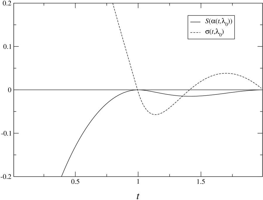
Figure 3: Plot of the dynamic entropy, $S(\alpha(t,\lambda_{0}))$, (solid curve) and entropy production rate, $\sigma(t,\lambda_{0})$, (dashed curve) versus time for an ideal gas with an a priori uniform velocity distribution with support on $[-1,1]$. The initial macrostate is $a_{0}=1\;(\lambda_{0}=\infty)$.

6 Discussion

We have considered the time evolution of a given set of macroscopic variables in a microscopically deterministic, isolated system. At equilibrium, these variables attain their most probable values but over time will exhibit fluctuations away from equilibrium. We have shown that for small fluctuations the most probable evolution of these fluctuations in the near future (and near past) is governed by the Onsager principle, which gives a linear relationship between the flows and thermodynamic forces. The former was interpreted as the time rate of change of the most probable macrostate, while the latter was found to correspond to the Legendre-transform conjugate of the initial, nonequilibrium macrostate. This result was obtained using well-established techniques from large deviation theory and is independent of any ad hoc mesoscopic time scale. An explicit expression for the forward and reverse Onsager matrices in terms of the covariance matrix of the macroscopic variables then followed.

The forward Onsager matrix was found to be positive semidefinite as a consequence of the assumed invariance of the a priori probability measure. The Onsager reciprocity relations were verified in the case of time reversal invarinace and found to imply that the forward and reverse Onsager matrices differ only by a sign. Together, these last two results imply that the second law of thermodynamics, as regards fluctuations, is valid in the aforementioned regime for both the forward and reverse time directions. Thus, given an initial nonequilibrium macrostate, a system’s initial tendency is to approach equilibrium (in the forward time direction) or to have arisen from a state closer to equilibrium (in the reverse time direction). This need not imply long-time approach to equilibrium, however, unless, for example, the macroscopic dynamics form a semigroup. At much later or earlier times, antithermodynamic behavior is also possible, as illustrated by the example considered of an ideal gas with a uniform velocity distribution.

References

- [1] S. Chapman and T. G. Cowling, The Mathematical Theory of Nonuniform Gases, Cambridge University Press, Cambridge, 1939.
- [2] S. R. de Groot, Thermodynamics of Irreversible Processes, North Holland, Amsterdam, 1951.
- [3] S. R. de Groot and P. Mazur, Non-Equilibrium Thermodynamics, North-Holland, Amsterdam, 1962.
- [4] L. Onsager, Phys. Rev. 37 (1931) 405.
- [5] L. Onsager, Phys. Rev. 38 (1931) 2265.
- [6] B. R. La Cour and W. C. Schieve, J. Stat. Phys. 107 (2002) 729.
- [7] B. R. La Cour and W. C. Schieve, J. Stat. Phys. 99 (2000) 1225.
- [8] A. Dembo and O. Zeitouni, Large Deviations Techniques and Applications, Jones and Bartlett, Boston, 1993.
- [9] J. Deuschel and D. W. Stroock, Large Deviations, Academic Press, San Diego, 1989.
- [10] R. S. Ellis, Entropy, Large Deviations, and Statistical Mechanics, Springer-Verlag, New York, 1985.
- [11] I. Prigogine, From Being to Becoming: Time and Complexity in the Physical Sciences, W. H. Freeman, San Francisco, 1980.
- [12] I. Prigogine, Introduction to Thermodynamics of Irreversible Processes, John Wiley, New York, 1967.
- [13] M. S. Green, J. Chem. Phys. 20 (1952) 1281.
- [14] H. B. G. Casimir, Rev. Mod. Phys. 17 (1945) 343.
- [15] H. Mori, Phys. Rev. 112 (1958) 1829.
- [16] E. Wigner, J. Chem. Phys. 22 (1954) 1912.
- [17] M. S. Green, J. Chem. Phys. 20 (1950) 1036.
- [18] R. Kubo, J. Phys. Soc. Japan 12 (1957) 570.
- [19] Y. Oono, Prog. Theor. Phys. 89 (1993) 973.
- [20] L. Bertini et al., J. Stat. Phys. 107 (2002) 645).
- [21] G. Gallavotti, Phys. Rev. Lett. 77 (1996) 4334.
- [22] G. Gallavotti and E. G. D. Cohen, Phys. Rev. Lett. 74 (1995) 2694.
- [23] G. Gallavotti and E. G. D. Cohen, J. Stat. Phys. 80 (1995) 931.
- [24] D. Gabrielli, G. Jona-Lasinio, and C. Landim, Phys. Rev. Lett. 77 (1996) 1202.
- [25] P. Ehrenfest and T. Ehrenfest, The Conceptual Foundations of the Statistical Approach in Mechanics, Cornell University Press, Ithaca, NY, 1959), english translation of the article published by B. G. Teubner (Leipzip, 1912) as No. 6 of Vol. IV 2 II of the Encyklopädie der mathematischen Wissenschaften.
- [26] M. Kogan, Rarefied Gas Dynamics, Plenum, New York, 1969.