Catacondensed Chemical Hexagonal Complexes:
A Natural Generalisation of Benzenoids

Abstract

Catacondensed benzenoids (those benzenoids having no carbon atom belonging to three hexagonal rings) form the simplest class of polycyclic aromatic hydrocarbons (PAH). They have a long history of study and are of wide chemical importance. In this paper, mathematical possibilities for natural extension of the notion of a catacondensed benzenoid are discussed, leading under plausible chemically and physically motivated restrictions to the notion of a catacondensed chemical hexagonal complex (CCHC). A general polygonal complex is a topological structure composed of polygons that are glued together along certain edges. A polygonal complex is flat if none of its edges belong to more than two polygons. A connected flat polygonal complex determines an orientable or nonorientable surface, possibly with boundary. A CCHC is then a connected flat polygonal complex all of whose polygons are hexagons and each of whose vertices belongs to at most two hexagonal faces. We prove that all CCHC are Kekulean and give formulas for counting the perfect matchings in a series of examples based on expansion of cubic graphs in which the edges are replaced by linear polyacenes of equal length. As a preliminary assessment of the likely stability of molecules with CCHC structure, all-electron quantum chemical calculations are applied to molecular structures based on several CCHC, using either linear or kinked unbranched catafused polyacenes as the expansion motif. The systems examined all have closed shells according to Hückel theory and all correspond to minima on the potential surface, thus passing the most basic test for plausibility as a chemical species. Preliminary indications are that relative energies of isomers are affected by the choice of the catafusene motif, with a preference shown for kinked over linear polyacenes, and for attachment by angular connection at the branching hexagons derived from the vertices of the underlying cubic structure. Avoidance of steric crowding of H atoms appears to be a significant factor in these preferences.

Keywords: Benzenoid, polygonal complex, (catacondensed) chemical hexagonal complex, Kekulé structure.

Math. Subj. Class. (2020): 05C92

Dedicated to Milan Randić on the occasion of his 90th birthday.

1 Introduction

The familiar classes of conjugated unsaturated hydrocarbon molecules, such as benzenoids, coronoids, helicenes and more general fusenes, may all be regarded in a mathematical sense as sets of graphs equipped with additional properties. In the simplest case, the hexagonal rings of such molecules may be considered as faces of a map on the plane. In this note we extend this notion by retaining the local properties of benzenoids but relaxing global planarity. Since the first isolation of benzene almost 200 years ago, benzenoids and their derivatives have had a significant, if not always benign, presence in the mainstream of organic chemistry and its applications. Mathematical study of benzenoids also has a long history, with central ideas [17, 1] contributed by pioneering experimental chemists such as Kekulé [44], Fries [33] and Clar [13, 14, 15] feeding into an enormous primary literature codified in influential textbooks [21, 20, 19, 41, 82]. The present paper is dedicated to another major figure, Milan Randić, whose ideas on the use of conjugated circuits [65] for the description of resonance energy have been influencing thinking in this area for nearly half a century [63, 24, 62, 69, 61, 39, 83, 3, 4, 5, 64]. Most recently, his simple but insightful picture of ring-current aromaticity of benzenoids has revived interest in ways of modelling and, especially, of interpreting molecular currents [35, 66, 68, 67, 70, 71, 12, 51, 29, 31, 30].

The simplest structures, with many applications in chemistry, are benzenoids. Graphene may be viewed as an infinite benzenoid. In this paper we are interested only in finite structures. There are several ways to describe a finite benzenoid: boundary-edges codes [38, 8, 22], inner duals [54, 42], flag-graphs [49, 59], or through the coordinates of the hexagons in the infinite hexagonal tesselation of the plane [6]. Benzenoids having no inner vertices (i.e.  no vertices common to three hexagons) are called catacondensed, whilst those having inner vertices are called pericondensed. Among catacondensed benzenoids we distinguish branched and unbranched benzenoids. The simplest unbranched benzenoids are linear benzenoids or linear polyacenes.

If the structures are allowed to spiral we call them helicenes. These are still planar, in the graph theoretical sense, and simply connected but no longer fit onto a hexagonal grid without overlap. The term fusenes covers both benzenoids and helicenes. Note that the boundary does not determine uniquely a general fusene; see for instance work by Brinkmann [9, 10].

Benzenoids with holes (i.e. those that are not simply connected) are coronoids. Again, those that have no internal vertices are catacondensed coronoids (or perhaps more simply, catacoronoids to correspond to catabenzenoids). Benzenoids and coronoids have both been considered as maps on a surface with boundary [49, 59, 7]. Fusenes can be further generalised to allow for structures that are not necessarily simply connected. In the literature, various generalizations to surfaces of higher genus have been made. For instance, torusenes (also called toroidal polyhexes or torenes) have been considered [46, 52, 47]. Since we may tile the Klein bottle by hexagons [23], we may also speak of kleinbottlenes. There is a whole menagerie of proposed finite and infinite theoretical carbon nanostructures, such as Möbiusenes, tubulenes, hexagonal systems, hexagonal animals, toroidal benzenoids, Schwarzites, Haeckelites, etc. [40, 73, 74, 81, 80, 79, 77, 78]. The theory of maps [36, 60] offers a toolbox for a general treatment of these diverse structures.

Note that each map on a surface determines a graph, called the skeleton of the map, that is obtained by discarding the faces of the map and retaining the vertices and edges. Whilst the skeleton is uniquely determined by the map, the converse is not true. A given graph may be a skeleton of several non-isomorphic maps. This fact has long been known to geometers: it was already Johannes Kepler who presented non-convex regular polyhedra [45]. For instance, the great dodecahedron has the same skeleton as the icosahedron. Another example is the skeleton of the tetrahedron, which is the complete graph $K_{4}$. The graph $K_{4}$ is also the skeleton of the hemihexahedron (also called hemicube), a map with three quadrilateral faces in the projective plane [16, 53]. In mathematical chemistry this problem is relevant when counting the number of distinct toroidal polyhexes. One has to choose whether to count graphs or maps. Pisanski and Randić [61] give the example of the cube graph ($Q_{3}$), which has two non-equivalent hexagonal embeddings in the torus; see also Figure 3 below.

In the next section, we present a flexible language for describing benzenoids and their many generalisations.

2 Polygonal complex

2.1 Scheme

Following Ringel [72], one can describe a cellular embedding of a graph in a closed surface by a scheme. Here we generalise Ringel’s approach in two directions. If we do not insist that each symbol appears exactly twice, we may use such schemes to describe the combinatorial structure of more general polygonal complexes in the sense of Schulte et al. [56, 57, 58, 75]. On the other hand, if we allow symbols with a single appearance, we may describe chemical structures, such as benzenoids as graphs embedded in a surface with a boundary.

Assume we are given a finite alphabet $A$. To each symbol $a\in A$ assign two literals $a^{+},a^{-}$. We say that $a^{+}$ is inverse of $a^{-}$ and that $a^{-}$ is inverse of $a^{+}$. Hence, if alphabet $A$ has $n$ symbols, there are $2n$ literals. When there is no ambiguity, we will write $a$ for $a^{+}$. A word over literals denotes an oriented polygon. A sequence of words, also called a scheme, denotes a polygonal complex, i.e. collection of polygons, some glued along their edges. A double appearance of a symbol represents the gluing. If the symbols appear in the same literal, the gluing is parallel; otherwise it is antiparallel. This terminology is used in the description of polyhedral self-assembly in synthetic biology [25, 48]. Usually, we present a scheme in a tabular form, where each row corresponds to a word.

Ringel [72] defines some operations on schemes that induce an equivalence relation such that two equivalent schemes define the same polygonal complex. Two schemes are equivalent if one can be obtained from the other by a sequence of transformations of the following types:

1. Permute the rows of a scheme (since we may always reorder the list of polygons);

2. Make a cyclic permutation of a row (since we may always start following the edges of a polygon from any of its vertices);

3. Replace any symbol by an unused symbol while keeping the exponents (since we may always relabel the edges of the polygonal complex);

4. Pick a symbol and replace each occurrence of a literal by its inverse (since we may always reverse the direction of any edge);

5. Reverse the row and simultaneously replace each literal by its inverse (since we may always reverse the orientation of any polygon).

A scheme may satisfy some additional properties. For example:

1. A scheme is connected if it cannot be divided into two disjoint sub-schemes that have no symbol in common;

2. A scheme is flat if each symbol appears at most twice in the scheme;

3. A scheme is closed if each symbol appears at least twice in the scheme;

4. A scheme is linear if each word that contains exactly two symbols that appear multiple times in the scheme has them in antipodal positions;

5. A scheme is chemical if, whenever $ab$ appears in the scheme such that $a$ and $b$ both have multiple appearance, then there exists a literal $c$ (different from $a$ and $b$) such that $b^{-}c$ (or, alternatively, $c^{-}b$) and $c^{-}a$ (or, alternatively, $a^{-}c$) appear in the same scheme;

6. A scheme is catacondensed if, whenever $ab$ appears in the scheme, then at least one of the symbols $a$ and $b$ appears only once;

7. A scheme is unbranched if every word of the scheme contains at most two symbols that appear more than once in the scheme and if there are two in a given word, they are non-adjacent. A catacondensed scheme is called branched whenever it is not unbranched;

8. A scheme is hexagonal if each word contains six literals;

9. A scheme is oriented if no literal appears in it twice (i.e. no symbol appears twice with the same exponent). It is orientable if it is equivalent to an oriented scheme. A scheme that is not orientable is nonorientable.

Note that (S4) implies (S7) and (S7) implies (S6). Also, every orientable scheme is flat. All properties (S1) – (S8) are preserved under the aforementioned transformations (T1) – (T5) and hence also apply to polygonal complexes. The property (S5) is equivalent to requiring that the skeleton graph is a chemical graph (i.e. has maximum degree less than or equal to $3$). The property ‘oriented’ (S9) is not preserved under (T5), though it is still preserved under (T1) – (T4). However, properties ‘orientable’ and ‘nonorientable’ are preserved under (T1) – (T5). We know that a connected flat scheme represents a compact surface with a boundary. The boundary is determined by symbols that appear only once in the scheme. If a connected flat scheme is also closed then the surface itself is closed, i.e. it has no boundary. With these definitions, a fullerene is a case of a closed chemical complex that is not hexagonal, since it has $12$ pentagonal faces [28].

Example 1.

A typical example of a polygonal complex in the sense of Schulte et al. [56, 57, 58, 75] is a $2$-dimensional skeleton of the tesseract (the $4$-dimensional cube). This skeleton is composed of $16$ vertices, $32$ edges and $24$ quadrilateral faces.

Figure 1: The tesseract showing edge labelling as in the scheme presented in Example 1.

The eight facets of the tesseract (which are all cubes) are discarded. A scheme describing the skeleton is given here (split into two columns for convenience):

$$\begin{matrix}[l]a&f&i^{-}&c^{-}\\ a&e&k^{-}&d^{-}\\ a&g&u^{-}&b^{-}\\ b&v&j^{-}&c^{-}\\ b&w&m^{-}&d^{-}\\ c&h&l^{-}&d^{-}\\ e&n&r&f^{-}\\ e&o&x^{-}&g^{-}\\ f&t&z^{-}&g^{-}\\ h&p&r&i^{-}\\ h&q&4&j^{-}\\ i&t&6^{-}&j^{-}\end{matrix} \begin{matrix}[l]k&n&p^{-}&l^{-}\\ k&o&y^{-}&m^{-}\\ l&q&1^{-}&m^{-}\\ n&s&2^{-}&o^{-}\\ p&s&3^{-}&q^{-}\\ r&t&5^{-}&s^{-}\\ u&x&y^{-}&w^{-}\\ u&z&6^{-}&v^{-}\\ v&4^{-}&1^{-}&w^{-}\\ z&5^{-}&2^{-}&x^{-}\\ 3&5&6^{-}&4^{-}\\ 1&3&2^{-}&y^{-}\end{matrix}$$ (1)

As we can see, each symbol appears three times, because each edge lies on the boundary of three quadrilaterals. Since the scheme is not flat it is nonorientable. Note that the $1$-skeleton, i.e. the skeleton graph of the tesseract, is the $4$-hypercube graph, $Q_{4}$. $\Diamond$

From now on, we will only consider flat polygonal complexes. Originally the term polygonal complex was reserved for flat polygonal complexes. See for instance chapter by Pisanski and Potočnik in [60]. More information about maps can be obtained from [37]. The following example shows how one can distinguish between a tetrahedron and a tetrahedron with one face missing.

Figure 2: Open and closed tetrahedra. The Schlegel diagram with the infinite face BCD included represents the closed tetrahedron. In the open tetrahedron the final triangular face $cfd$ ($BCD$) has been removed.

Example 2.

Consider the scheme:

$$\Theta=\;\begin{matrix}[l]a&b&c\\ a^{-}&f&e\\ b^{-}&e^{-}&f\\ f^{-}&c^{-}&d^{-}\end{matrix}$$ (2)

This represents a tetrahedron. There are six edges and each row corresponds to a triangular face. All symbols in $\Theta$ appear twice, and hence the corresponding surface is closed (has no boundary). The surface in this case is a sphere. By removing a face, for instance the last one, we obtain a connected scheme:

$$\Theta^{\prime}=\;\begin{matrix}[l]a&b&c\\ a^{-}&e&e\\ b^{-}&e^{-}&f\end{matrix}$$ (3)

that represents a tetrahedron with one face missing. The symbols $c,d,f$ each occur only once and the corresponding surface is a disk. $\Diamond$

(a) $\Sigma$

(b) $\Sigma^{\prime}$

(c) $\Sigma^{\prime\prime}$

Figure 3: Three embeddings of the cube graph $Q_{3}$.

Example 3.

Here are three maps that all have the same skeleton, namely the cube graph, $Q_{3}$:

$$\Sigma=\;\begin{matrix}[l]a&b&c&d\\ h^{-}&g^{-}&f^{-}&e^{-}\\ a^{-}&i&e&j^{-}\\ j&f&k^{-}&b^{-}\\ g&l^{-}&c^{-}&k\\ d^{-}&l&h&i^{-}\end{matrix}$$ (4)

$$\Sigma^{\prime}=\;\begin{matrix}a&b&k&f^{-}&e^{-}&i^{-}\\ c&d&i&h^{-}&g^{-}&k^{-}\\ f&g&l^{-}&c^{-}&b^{-}&j\\ h&e&j^{-}&a^{-}&d^{-}&l\end{matrix}$$ (5)

$$\Sigma^{\prime\prime}=\;\begin{matrix}a&b&k&g&h&i^{-}\\ c&d&i&e&f&k^{-}\\ l&g^{-}&f^{-}&j^{-}&a^{-}&d^{-}\\ b&c&l&h&e&j^{-}\end{matrix}$$ (6)

Note that $\Sigma$ describes the usual hexahedron, i.e. the surface of the cube. $\Sigma^{\prime}$ and $\Sigma^{\prime\prime}$ describe two non-equivalent toroidal polyhexes. All three maps share the same underlying skeleton, the cube graph $Q_{3}$. However, the embeddings $\Sigma^{\prime}$ and $\Sigma^{\prime\prime}$ are clearly distinct. $\Sigma^{\prime\prime}$ has the property that each pair of faces intersects in exactly two edges which are antipodal in each face, whereas $\Sigma^{\prime}$ does not. $\Sigma^{\prime\prime}$ is a regular map [16, 53], a generalisation of Platonic polyhedra.

$\Diamond$

The above example raises an interesting question: Which toroidal polyhexes are completely determined by their skeleta?

3 Equilinear catacondensed chemical hexagonal complexes

Catacondensed chemical hexagonal complexes are characterized by the following rules: they are connected (S1), flat (S2), hexagonal (S8) and catacondensed (S6). These rules imply that such a complex is also chemical (S5). We may view such a complex as a collection of branching hexagons that are connected by chains of hexagons. If each hexagonal chain is linear (property (S4) holds for the complex), we say that such a structure is a linear catacondensed chemical hexagonal complex. Moreover, if all linear hexagonal chains are of the same length, i.e. contain the same number of hexagons, these structures are called equilinear. We denote by $l$ the common length of these linear chains.

In the unbranched case (where (S7) holds), for a given $l$, there are only three catacondensed structures: $P_{l},C_{l}$ and $M_{l}$, as illustrated in Figure 4.

Figure 4: Unbranched catacondensed chemical hexagonal complexes: (a) linear polyacene $P_{6}$, (b) untwisted cyclacene $C_{6}$, and (c) Möbius cyclacene $M_{6}$. For the two cyclacene cases, the arrowed left and right edges are to be identified.

In the branched case, there are three types of hexagon: branching (attached to three hexagons, i.e. of type $A_{3}$ in the notation of [41]), connecting (attached to two hexagons, i.e. of type $A_{2}$ or $L_{2}$), and terminal (attached to a single hexagon, i.e. of type $L_{1}$). Such a structure defines a labelled 1-3 map (i.e. vertices are of degrees $1$ and $3$), called the blueprint map. A map is a graph together with a rotation projection [36]. The underlying graph is called the blueprint graph. In the map, each arc is labelled by a pair $(w,\sigma)$, where $w$ is a word over the alphabet $\{L,R,S\}$ and $\sigma\in\{+,-\}$. The reverse of a label $(w,\sigma)$ is the label $(w^{\rho},\sigma)$, where $w^{\rho}$ is the reverse of the word in which symbols $L$ and $R$ are interchanged. Labels are assigned to arcs (half-edges) and two opposite arcs are assigned reverse labels. For instance, reverse of the label $(RLSR,+)$ is the label $(LSRL,+)$. Degree $3$ vertices correspond to branching hexagons, while vertices of degree $1$ correspond to terminal hexagons. The connecting hexagons are implicitly described by the labels; see Figure 5.

Figure 5: Arc labelling in the blueprint map. In the untwisted (a) and the twisted (b) the word $w$ is $RLSR$ taken in the direction from bottom to top or $LSRL$ from top to bottom, whilst $\sigma=+$ and $\sigma=-$, respectively.

In the equilinear case, the description given above can be simplified. Words in labels on arcs comprise only the letter $S$. Therefore each word can be described by giving its length, and then only one integer parameter is needed.

Figure 6 shows rotation projections for all blueprint maps on up to two trivalent vertices. Note that in the case of zero vertices of degree $3$, two cases are anomalous, as they are free loops with no vertices at all.

(a) Zero vertices of degree $3$:

$\mathcal{M}_{1,0}^{0}$           $\mathcal{M}_{2,0}^{0}$           $\mathcal{M}_{2,1}^{0}$

(b) One vertex of degree $3$:

$\mathcal{M}_{1,0}^{1}$           $\mathcal{M}_{2,0}^{1}$           $\mathcal{M}_{2,1}^{1}$

(c) Two vertices of degree $3$, one connecting edge:

$\mathcal{M}_{1,0}^{2}$       $\mathcal{M}_{2,0}^{2}$       $\mathcal{M}_{2,1}^{2}$       $\mathcal{M}_{3,0}^{2}$       $\mathcal{M}_{3,1}^{2}$       $\mathcal{M}_{3,2}^{2}$

(d) Two vertices of degree $3$, two connecting edges:

$\mathcal{M}_{4,0}^{2}$           $\mathcal{M}_{4,1}^{2}$           $\mathcal{M}_{5,0}^{2}$           $\mathcal{M}_{5,1}^{2}$

(e) Two vertices of degree $3$, three connecting edges:

$\mathcal{M}_{6,0}^{2}$           $\mathcal{M}_{6,1}^{2}$           $\mathcal{M}_{7,0}^{2}$           $\mathcal{M}_{7,1}^{2}$

Figure 6: The blueprint maps with $n\leq 2$ trivalent vertices. The symbol on an edge represents a half-twist. In maps $\mathcal{M}_{7,0}^{2}$ and $\mathcal{M}_{7,1}^{2}$ the crossing edges are necessary, because the order of edges around a vertex is significant and cannot be represented in a planar drawing.

4 Kekulé structures in catacondensed coronoid complexes

A natural question to ask is which flat hexagonal complexes admit a Kekulé structure. It is well known that all catacondensed benzenoids are Kekulean [41].

Theorem 1.

Any catacondensed flat hexagonal complex $B$ is Kekulean.

Note that any catacondensed flat hexagonal complex is also a chemical hexagonal complex.

Proof.

The proof is constructive – we construct a perfect matching $\mathcal{M}$. A catacondensed flat hexagonal complex contains only hexagons of type $L_{1}$, $L_{2}$, $A_{2}$ and $A_{3}$ (see [41, p. 21]). In the first step we remove all hexagons of type $A_{3}$ from $B$. Edges labelled $a,b$ and $c$ in Figure 7 will be single bonds (they are not in the matching $\mathcal{M}$). By removing a hexagon of type $A_{3}$ we mean deleting edges $a$, $b$ and $c$.

Figure 7: Types of hexagons in catafused flat hexagonal complex $B$.

In the second step we remove all hexagons of type $A_{2}$ from $B$. Edges labelled $a,b$ and $c$ in Figure 7 will be single bonds, whilst the edge $d$ will be double (we add it to $M$).

Figure 8: The complex $B$ after deletion of hexagons of types $A_{3}$ and $A_{2}$.

What remains is a disjoint union of $k$ linear polyacene chains $P^{i}$ (see Figure 8(a)) which may be of different lengths, $p$ untwisted cyclacenes $C^{i}$ (see Figure 8(a)), $q$ twisted cyclacenes $T^{i}$ (see Figure 8(b)), and $m$ isolated $K_{2}$ fragments:

$$\{P^{1},P^{2},\ldots,P^{k}\}\cup\{C^{1},C^{2},\ldots,C^{p}\}\cup\{M^{1},M^{2},\ldots,M^{q}\}\cup\{K_{2}^{1},K_{2}^{2},\ldots,K_{2}^{r}\}.$$

We add all isolated $K_{2}$ fragments to the perfect matching $\mathcal{M}$. All linear chains and cyclacenes are Kekulean. For each chain we may pick any of $l_{i}+1$ perfect matchings. An untwisted cyclacene has $4$ perfect matchings, and a twisted cyclacene has $2$ perfect matchings, hence $K(B)\geq 4^{p}2^{q}\prod_{i=1}^{k}(l_{i}+1).$ ∎

Figure 9: Basic Rules for perfect matchings of hexagonal complexes derived with linear polyacene strips (illustrated for strips of length $3$). They are: (a) the linear forcing rule; (b) the crossover rule; (c) the pairing rule. Hexagons A and B are derived from cubic vertices. Fixing the illustrated endo bonds of hexagon A (denoted $d$ or $s$ for double or single) either forces (rules (a) and (b)) or rules out ((c)) given pairings of the corresponding endo bonds in hexagon B. The panels show (left) the untwisted chain and (right) the chain with a Möbius half-twist.

This reasoning can be used as the basis of a simple procedure for counting the perfect matchings for a flat hexagonal complex with a given rotation scheme. For the linear polyacene motif, this leads to polynomial functions in $l+1$. The detailed form of these expressions, the powers that appear and the coefficients that multiply them can be rationalised by thinking about a set of forcing rules for replacements of edges of the cubic graph by linear chains of polyacenes. In this case, three rules apply to allowed combinations of pairs of edges in the two branching hexagons (see Figure 9). Rule (a) is the linear forcing rule, by which two double bonds in A force a fixed matching in the chain and two single bonds in B. Rule (b) is the crossover rule, by which a single/double pair in A forces a fixed matching in the chain and a double/single pair in B. Rule (c) is the pairing rule, by which a pair of single bonds in A is compatible with either a pair of single bonds or a pair of double bonds in B. The pair of single bonds in B results from taking any of the $(l+1)$ perfect matchings of the intervening hexagons. The pair of double bonds of B arises from reversal of the linear forcing rule. (A single/double pair in B is ruled out by the crossover rule.)

Note that if we make a complex from a cubic graph with $m$ edges by using a straight chain of length $l$ on every edge, there is a term $(l+1)^{m}$ in the Kekulé count. Kinks in the chains will increase this leading term [2, 27]. E.g. fibonacene chains of length $l$ would lead to a term $(F_{l+2})^{m}$, where $F_{l+2}$ is the $(l+2)$-th Fibonacci number. Fibonacene chains also allow favourable perfect matchings in which there are many hexagonal rings containing three double bonds, thus conforming to classical models of stability based on the ideas of Fries [33] and Clar [15]; see Figure 10.

Figure 10: A fully Fries hexagonal complex, i.e. one in which every hexagonal face includes three matched edges, can be constructed by using either an odd or or an even zig-zag fibonacene to inflate all edges of a cubic graph. Several attachment isomers are possible: for example, a fully Fries attachment isomer could be built using any external double bond in each terminal hexagon.

Some explicit formulas for Kekulé counts of complexes built from cubic graphs and linear polyacenes are:

$\mathcal{T}_{0,0}$ $\mathcal{T}_{0,1}$ $\mathcal{T}_{0,2}$ $\mathcal{T}_{0,3}$

$\mathcal{T}_{1,0}$ $\mathcal{T}_{1,1}$ $\mathcal{T}_{1,2}$ $\mathcal{T}_{1,3}$

$\mathcal{T}_{2,0}$ $\mathcal{T}_{2,1}$ $\mathcal{T}_{2,2}$ $\mathcal{T}_{2,3}$

Figure 11: Maps derived from the embeddings of the graph $K_{4}$, with and without twists. Only $9$ of the $12$ drawings shown here are distinct, as $(\mathcal{T}_{0,3},\mathcal{T}_{2,3})$, $(\mathcal{T}_{1,1},\mathcal{T}_{2,2})$, and $(\mathcal{T}_{1,2},\mathcal{T}_{2,1})$ are isomorphic pairs. Conventions for edges as in Figure 6.

1. For the theta graph for all distinct embeddings and sets of twists:

   $$K(\mathcal{M}_{6,0}^{2};l) ={\left(l+1\right)}^{3}+8$$ (7)

   $$K(\mathcal{M}_{6,1}^{2};l) ={\left(l+1\right)}^{3}+4$$ (8)

   $$K(\mathcal{M}_{7,0}^{2};l) ={\left(l+1\right)}^{3}+3\,(l+1)+2$$ (9)

   $$K(\mathcal{M}_{7,1}^{2};l) ={\left(l+1\right)}^{3}+(l+1)+2$$ (10)

2. For the tetrahedron for all distinct embeddings and sets of twists:

   $$K(\mathcal{T}_{0,0};l) ={\left(l+1\right)}^{6}+4\,{\left(l+1\right)}^{3}+3\,{\left(l+1\right)}^{2}$$ (11)

   $$K(\mathcal{T}_{0,1};l) ={\left(l+1\right)}^{6}+4\,{\left(l+1\right)}^{3}+3\,{\left(l+1\right)}^{2}+2\,(l+1)$$ (12)

   $$K(\mathcal{T}_{0,2};l) ={\left(l+1\right)}^{6}+4\,{\left(l+1\right)}^{3}+2\,{\left(l+1\right)}^{2}+3\,(l+1)$$ (13)

   $$K(\mathcal{T}_{0,3};l)=K(\mathcal{T}_{2,3};l) ={\left(l+1\right)}^{6}+5\,{\left(l+1\right)}^{3}+3\,{\left(l+1\right)}^{2}+6\,(l+1)+2$$ (14)

   $$K(\mathcal{T}_{1,0};l) ={\left(l+1\right)}^{6}+4\,{\left(l+1\right)}^{3}+3\,(l+1)$$ (15)

   $$K(\mathcal{T}_{1,1};l)=K(\mathcal{T}_{2,2};l) ={\left(l+1\right)}^{6}+5\,{\left(l+1\right)}^{3}+{\left(l+1\right)}^{2}+2\,(l+1)+2$$ (16)

   $$K(\mathcal{T}_{1,2};l)=K(\mathcal{T}_{2,1};l) ={\left(l+1\right)}^{6}+4\,{\left(l+1\right)}^{3}+2\,{\left(l+1\right)}^{2}+2\,(l+1)+2$$ (17)

   $$K(\mathcal{T}_{1,3};l) ={\left(l+1\right)}^{6}+4\,{\left(l+1\right)}^{3}+5\,{\left(l+1\right)}^{2}+4\,(l+1)+4$$ (18)

   $$K(\mathcal{T}_{2,0};l) ={\left(l+1\right)}^{6}+4\,{\left(l+1\right)}^{3}+4$$ (19)

3. For the cube in the usual embedding, $\Sigma$ (see Figure 3(a)), on the sphere, with no twist and one twisted edge, and for the untwisted toroidal embeddings, $\Sigma^{\prime}$ and $\Sigma^{\prime\prime}$ (see Figures 3(b) and 3(c)), respectively:

   $$K(\Sigma_{0};l) ={\left(l+1\right)}^{12}+8\,{\left(l+1\right)}^{9}+32\,{\left(l+1\right)}^{6}+64\,{\left(l+1\right)}^{3}+64$$ (20)

   $$K(\Sigma_{1};l) ={\left(l+1\right)}^{12}+8\,{\left(l+1\right)}^{9}+26\,{\left(l+1\right)}^{6}+40\,{\left(l+1\right)}^{3}+32$$ (21)

   $$K(\Sigma^{\prime}_{0};l) ={\left(l+1\right)}^{12}+8\,{\left(l+1\right)}^{9}+2\,{\left(l+1\right)}^{8}+24\,{\left(l+1\right)}^{6}+8\,{\left(l+1\right)}^{5}$$ (22)

   $$\quad{}+17\,{\left(l+1\right)}^{4}+32\,{\left(l+1\right)}^{3}+8\,{\left(l+1\right)}^{2}+16$$

   $$K(\Sigma^{\prime\prime}_{0};l) ={\left(l+1\right)}^{12}+8\,{\left(l+1\right)}^{9}+6\,{\left(l+1\right)}^{8}+16\,{\left(l+1\right)}^{6}+24\,{\left(l+1\right)}^{5}$$ (23)

   $$\quad{}+9\,{\left(l+1\right)}^{4}+16\,{\left(l+1\right)}^{3}+24\,{\left(l+1\right)}^{2}+16$$

4. For the dodecahedron on the sphere, with no twist and one twisted edge, respectively:

   $$K(\mathcal{D}_{0};l) ={\left(l+1\right)}^{30}+20\,{\left(l+1\right)}^{27}+160\,{\left(l+1\right)}^{24}+660\,{\left(l+1\right)}^{21}+36\,{\left(l+1\right)}^{20}$$ (24)

   $$\quad{}+1510\,{\left(l+1\right)}^{18}+360\,{\left(l+1\right)}^{17}+1972\,{\left(l+1\right)}^{15}+1260\,{\left(l+1\right)}^{14}$$

   $$\quad{}+120\,{\left(l+1\right)}^{13}+1560\,{\left(l+1\right)}^{12}+1800\,{\left(l+1\right)}^{11}+636\,{\left(l+1\right)}^{10}$$

   $$\quad{}+660\,{\left(l+1\right)}^{9}+1020\,{\left(l+1\right)}^{8}+600\,{\left(l+1\right)}^{7}+125\,{\left(l+1\right)}^{6}$$

   $$K(\mathcal{D}_{1};l) ={\left(l+1\right)}^{30}+20\,{\left(l+1\right)}^{27}+160\,{\left(l+1\right)}^{24}+2\,{\left(l+1\right)}^{23}+2\,{\left(l+1\right)}^{22}$$ (25)

   $$\quad{}+660\,{\left(l+1\right)}^{21}+52\,{\left(l+1\right)}^{20}+24\,{\left(l+1\right)}^{19}+1512\,{\left(l+1\right)}^{18}$$

   $$\quad{}+394\,{\left(l+1\right)}^{17}+124\,{\left(l+1\right)}^{16}+1984\,{\left(l+1\right)}^{15}+1250\,{\left(l+1\right)}^{14}$$

   $$\quad{}+428\,{\left(l+1\right)}^{13}+1608\,{\left(l+1\right)}^{12}+1738\,{\left(l+1\right)}^{11}+936\,{\left(l+1\right)}^{10}$$

   $$\quad{}+848\,{\left(l+1\right)}^{9}+984\,{\left(l+1\right)}^{8}+708\,{\left(l+1\right)}^{7}+285\,{\left(l+1\right)}^{6}+50\,{\left(l+1\right)}^{5}$$

   We note in passing that the corresponding formula for the untwisted embedding of the Petersen graph in the projective plane, which is admittedly of less chemical interest, is

   $$K(\text{Petersen};l)={\left(l+1\right)}^{15}+10\,{\left(l+1\right)}^{12}+30\,{\left(l+1\right)}^{9}+55\,{\left(l+1\right)}^{6}+55\,{\left(l+1\right)}^{3}$$ (26)

5. For the $k$-prism $\mathcal{R}^{k}$:

   For $k$ odd, the prism with linear polyacene motifs, embedded on the sphere without a twist has

   $$K(\mathcal{R}^{k}_{0};l)=((l+1)^{3}+2)^{k}-2^{k}$$ (27)

   and for $k$ even it has

   $$K(\mathcal{R}^{k}_{0};l)=[((l+1)^{3}+2)^{k/2}+2^{k/2}]^{2}$$ (28)

We note that as the rules (a) to (c) apply without change to the limiting case of $l=0$ hexagons in the linear polyene chain, the formulas for the untwisted chains apply to the leapfrog [26] of an embedded cubic graph and hence give the Kekulé count of the leapfrog by summation of coefficients of all powers of $(l+1)$. For example, the formula for the untwisted dodecahedron $\mathcal{D}_{0}$ gives the number of Kekulé structures of the icosahedral C₆₀ fullerene as $K(\mathcal{D}_{0};0)=12500$. Simple results are also found for the numbers of perfect matchings of leapfrog prisms, namely $3^{k}-2^{k}$ and $(3^{k/2}+2^{k/2})^{2}$. The prism itself has Kekulé count given by sequence A068397 [55], i.e. $K$ for the $k$-prism is $F(k+1)+F(k-1)+(-1)^{k}+1$.

5 Structural calculations

This section connects the foregoing mathematical development with possible realisations of new unsturated hydrocarbon frameworks. Graph theoretical considerations based on Kekulé counts, HOMO-LUMO gap and $\pi$ energy can be valuable indicators of stability of a $\pi$ system. In particular, it is useful to know if a $\pi$ system is predicted to have a closed shell (in which all electrons are paired) and to characterise such shells in terms of whether this electron configuration is properly closed (having all bonding orbitals occupied and all antibonding orbitals empty). HOMO-LUMO maps [32, 43] can give a useful picture of trends in frontier-orbital energies and shell types for families of molecules. However, for a more reliable estimate of the prospects for overall stability of an unsaturated hydrocarbon C_xH_y it is necessary to take into account the full range of steric and electronic effects arising from both $\sigma$ and $\pi$ electronic subsystems. This section reports a selection of preliminary all-electron structural calculations using standard quantum chemical methods for various examples of chemical hexagonal complexes. They serve to show that this generalisation of benzenoids is chemically as well as mathematically plausible, and give clues to some of the factors that can influence absolute and relative stabilities. The systems chosen for study are linear polyacene expansions of the three cubic Platonic polyhedra, and a wider choice of isomeric expansions of the simplest cubic graph, the theta graph (see Figure 12). All these structures correspond to the standard embedding on the sphere; twisted systems and alternative embeddings were left for future investigations.

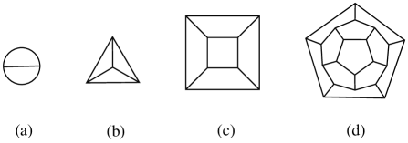
Figure 12: Cubic graphs used as the basis for flat hexagonal complexes: (a) the theta graph, (b) the tetrahedron, (c) the cube, (d) the dodecahedron. In cases (b) to (d), each edge is decorated with an anthracene chain; for case (a) see Figures 13, 14 and 15.

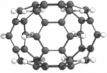
(a)

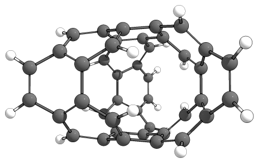
(b)

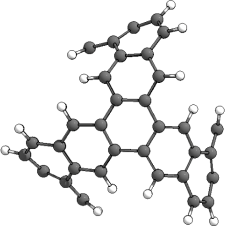
(c)

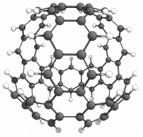
(d)

Figure 16: Ball-and-stick representations of some optimised molecular structures based on hexagonal complexes. (a) Isomer of C₄₂H₁₈ based on the anthracene expansion of the theta graph shown in Figure 13(a); (b) Isomer of C₄₂H₁₈ based on the phenanthrene expansion Pb of the theta graph (see Figure 14(b); (c) Top view of C₆₆H₃₀ isomer based on the fibonacene expansion of the theta graph shown in Figure 15(b); (d) View down the two-fold axis of a hexagonal complex, C₈₄H₃₆, based on the anthracene expansion of the tetrahedron.

In each case, the structure was optimised at the DFT level using the B3LYP functional and, in all but one, the 6-31G* basis for C and 6-31G for H. (In the case of the dodecahedral complex, C₄₂₀H₁₈₀, the basis was reduced to 6-31G for all atoms, on grounds of computational cost.) Candidate minima were checked in most cases in the usual way, by diagonalization of the Hessian. (For the largest cases, of the expanded cube and dodecahedron, stability of the candidate minimum structure was checked by relaxation of several nearby unsymmetrically perturbed structures.) Calculations were carried out with the QChem and Gaussian 16 packages [76, 34]. Energies and lowest harmonic frequencies are reported in Tables 1 and 2, together with geometric parameters and three graph invariants (Kekulé count, Hückel binding energy per carbon atom, and Hückel HOMO-LUMO gap). Snapshots of some optimised structures are shown in Figure 16.

Base graph	$l$	Formula	$K$	$(E_{\pi}/n)\beta$	$\Delta_{HL}\beta$	$E$/eV	$\tilde{\nu}/\text{cm}^{-1}$
Theta graph	$3$	C42H18	72	$1.439933$	$0.54778$	$-43836.415$	$76$
	$4$	C54H24	133	$1.431856$	$0.39425$	$-56381.449$	$52$
	$5$	C66H30	224	$1.426646$	$0.29932$	$-68925.208$	$34$
Tetrahedron	$3$	C84H36	4356	$1.439017$	$0.56885$	$-175391.522$	$39$
Cube	$3$	C168H72	19009600	$1.443904$	$0.54778$	$-175390.812$	—
Dodecahedron	$3$	C420H180	1561300213688815616	$1.439049$	$0.55627$	$-438398.859$	—

Table 1: Hexagonal chemical complexes based on inflation of cubic graphs with linear polyacene chains along edges. All isomers are based on linear annelation to alternate edges of the branching hexagons corresponding to vertices of the cubic graph. $l$ is the length of the chain motif, $K$ is the number of Kekulé structures, $(E_{\pi}/n)$ is the Hückel $\pi$ energy per carbon centre, in units of the $\beta$ resonance parameter, $\Delta_{HL}$ is the Hückel HOMO-LUMO gap, in the same units, $E$ is the total all-electron energy in eV (see text for the level of theory), and $\tilde{\nu}$ is the wavenumber in units of cm^-1 of the vibrational mode of lowest energy.

Formula	Isomer	$K$	$(E_{\pi}/n)\beta$	$\Delta_{HL}\beta$	$E$/eV	$\Delta E$/eV	$\tilde{\nu}/\text{cm}^{-1}$
C42H18	Aa	72	$1.439933$	$0.54778$	$-43836.415$	1.789	$76$
	Ab	108	$1.445495$	$0.81078$	$-43837.062$	1.142	$117$
	Ac	144	$1.450217$	$0.85153$	$-43836.830$	1.373	$70$
	Ad	144	$1.450269$	$0.85153$	$-43836.782$	1.422	$118$
	Pa	208	$1.455866$	$1.09287$	$-43834.363$	3.840	$74$
	Pb	160	$1.450380$	$1.09287$	$-43838.204$	0.000	$117$
	Pc	208	$1.456138$	$1.09287$	$-43836.842$	1.362	$124$
	Pd	176	$1.452603$	$1.09287$	$-43836.495$	1.708	$102$
	Pe	208	$1.455940$	$1.09287$	$-43835.822$	2.382	$136$
	Pf	176	$1.452827$	$1.03801$	$-43837.000$	1.204	$102$
C66H30	Fa	224	$1.426646$	$0.29932$	$-68925.208$	2.610	$34$
	Fb	1088	$1.436307$	$0.75569$	$-68927.219$	0.599	$52$
	Fc	2500	$1.444639$	$0.91215$	$-68927.818$	0.000	$50$

Table 2: Attachment isomers of hexagonal chemical complexes based on inflation of the theta graph with catafusenes composed of $3$ and $5$ hexagons (for formulas C₄₂H₁₈ and C₆₆H₃₀, respectively). The isomers are depicted in Figures 14 and 15. $K$ is the number of Kekulé structures, $(E_{\pi}/n)$ is the Hückel $\pi$ energy per carbon centre, in units of the $\beta$ resonance parameter, $\Delta_{HL}$ is the Hückel HOMO-LUMO gap, in the same units, $E$ is the total all-electron energy in eV (see text for the level of theory), and $\tilde{\nu}$ is the wavenumber in units of cm^-1 of the vibrational mode of lowest energy.

Structures based on the theta graph (Figure 12(a)) with all edges inflated to linear polyacene chains of $l$ hexagons were optimised successively for chains of length $l=3,4,5$. These correspond to molecular formulas C₄₂H₁₈, C₅₄H₂₄, and C₆₆H₃₀, respectively. All were found to occupy minima on the potential energy surface within the model chemistry. The optimised structures are barrels, with CC bond lengths in the expected range for polycyclic aromatic systems in this model chemistry,

Figure 13: A ‘polymer’ molecular notation for (a) anthracene and (b) phenanthrene expansions of the theta graph into flat hexagonal complexes of formula C₄₂H₁₈. Each monomer is to be repeated twice more to give a cyclic molecular structure with three-fold symmetry, topped and tailed by a hexagonal ring. Only graph vertices corresponding to carbon atoms are shown: vertices of degree two each carry a single H atom, and the graph is filled out with an appropriate Kekulé system of double bonds. The illustrated isomers are those denoted Aa and Pf, respectively, in the notation of Figure 14.

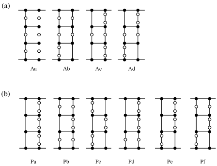
Figure 14: Schematic notation for attachment isomers of three-hexagon catafusene expansions of the theta graph. Each vertical block represents a possible strip in a three-fold symmetric isomer based on either anthracene (A) or phenanthrene (P). Notation: a black circle denotes a C centre that has three C neighbours; a white circle denotes a C centre that has two C neighbours and one H neighbour. For simplicity, the catafusene strip is shown as vertical; in the molecule the strip must bend in order to keep parallel the median planes of the hexagons centred on the C₃ axis of the hexagonal complex. Double bonds can be added, for example in any way consistent with internal Kekulé structures of the parent catafusene.

and low-frequency vibrational modes consistent with the flexibility expected of their open cage structures. Attempts to optimise the putative molecule with $l=2$, C₃₀H₁₂, failed to yield converged structures that corresponded to the initial molecular graph. The equivalent inflations using $l=3$ with the three cubic polyhedra (Figure 12) were also used to generate optimised molecular structures with formulas C₈₄H₃₆, C₁₆₈H₇₂, and C₄₂₀H₁₈₀, respectively (see Table 1 and Figure 12).

Figure 15: Two isomers of hexagonal complexes based on decoration of the theta graph with five-hexagon catafusenes. The diagrams represent three-fold symmetric decorations of the graph with (a) a singly kinked polyacene chain (Fb), and (b) a zig-zag fibonacene chain (Fc). Double bonds can be filled in ad lib to correspond with internal perfect matchings of the respective catafusenes. Both isomers share molecular formula C₆₆H₃₀ with the straight-chain isomer (Fa).

Whilst these results are already encouraging, it is not to be expected that the use of the mathematically simple linear polyacene fragments to inflate graph edges will automatically lead to the isomer of the hexagonal complex that has the highest chemical stability. There are at least two variations to the construction recipe that might be expected on electronic and/or steric grounds to improve stability. The more obvious of these is that for $l\geq 3$ we have choice for the isomer of the catafused benzenoid to be used in the inflation procedure. Considered as isolated molecules, bent catafusenes are typically more stable than their linear counterparts. Figure 13 illustrates this degree of freedom for the $l=3$ expansions of the theta graph, where phenanthrene offers a plausible alternative to anthracene. However, even once we fix on a given catafusene as our favoured structural motif, there are still different possibilities for its mode of annelation to the branch-point hexagons (of type $A_{3}$) that represent the vertices of the original cubic graph. We can, for example, construct ‘attachment isomers’ by choosing any contiguous pair $-$CH$-$CH$-$ on the catafusene perimeter as the site of the shared connection with the branch-point hexagonal ring. Figure 14 illustrates the variety of possible attachment isomers for the case of three-hexagon chains, with the added constraint of threefold rotational symmetry around the branching hexagons.

Optimisation shows that both variations on the basic recipe for construction are significant (see Table 2). Compared to direct linear annelation, the linear anthracene fragment gives a more stable isomer when attached to the branching hexagons in non-linear fashion (Ab). However, a further improvement in total energy comes from switching to the phenanthrene motif in the construction of the complex, again with a significant energetic preference for one particular attachment mode (Pb).

Preference for a phenanthrene over an anthracene motif is consistent with the relative stabilities of the isomeric C₁₄H₆ compounds [50]. Higher stability of the bent polyacene system is attributed in part to $\pi$ resonance effects, although these are hard to quantify uniquely [11, 18], and are offset by steric effects, such as H-H repulsion in the bay region. The computed relative energy of $1.142$ eV ($\sim 110$ kJ mol^-1) of isomers Ab and Pb, each containing three copies of the respective motifs, is compatible with the differential stability estimated from the difference of $23$ kJ mol^-1 in the standard formation enthalpies of the pure compounds [50], but points to a significant role for relief of steric crowding in the more open structure of the phenanthrene hexagonal complex Pb (see Figure 14 (b)). In support of this hypothesis of a major role for steric effects, we note that the indicators of pure $\pi$ electronic stability do not show any clear correlation with the computed relative energies of attachment isomers (Table 2, Aa-Ad, Pa-Pf). For example, whilst it is true that the isomer Pb, which has the lowest all-electron energy, has a higher Kekulé count, larger $\pi$ energy per electron and bigger HOMO-LUMO gap than its nearest competitor, Ab, it does not stand out on any of qualitative measures from the mass of the phenanthrenoid and anthracenoid isomers. Again, Pb has a large but not maximum Fries number. An overall trend to lower $\pi$ energy per electron and smaller HOMO-LUMO gap, countered by a rapidly increasing Kekulé count, is evident for CHCCs with longer linear polyacene motifs, and frequency calculations suggest increasing flexibility in larger cages with longer catafusene motifs.

These considerations may also be promising for the prospects of larger hexagonal complexes based on cubic polyhedra, where the face sizes are typically larger, and there should be more room for avoidance of steric clashes. With larger faces and longer chains, the complexes with twisted Möbius catafusenes along polyhedral edges may also become less sterically disfavoured. There are clearly many possibilities to be explored. Although by no means complete, this short survey has shown that at least some generalised hexagonal complexes survive the initial test of chemical plausibility in that they occupy minima on the potential surface. Synthetic accessibility is of course another matter.

References

- [1] J. W. Armit and R. Robinson, CCXI.—Polynuclear heterocyclic aromatic types. Part II. Some anhydronium bases, J. Chem. Soc. Trans. 127 (1925), 1604–1618, doi:10.1039/ct9252701604.
- [2] A. T. Balaban, Chemical graphs. L. Symmetry and enumeration of fibonacenes (unbranched catacondensed benzenoids isoarithmic with helicenes and zigzag catafusenes), MATCH Commun. Math. Comput. Chem. 24 (1989), 29–38.
- [3] A. T. Balaban and M. Randić, Partitioning of -electrons in rings of polycyclic conjugated hydrocarbons. VI. Comparison with other methods for estimating the local aromaticity of rings in polycyclic benzenoids, J. Math. Chem. 37 (2005), 443–453, doi:10.1007/s10910-004-1114-z.
- [4] A. T. Balaban and M. Randić, Perfect matchings in polyhexes, or recent graph-theoretical contributions to benzenoids, J. Univers. Comput. Sci. 13 (2007), 1514–1539, doi:10.3217/jucs-013-11-1514.
- [5] A. T. Balaban, M. Randić and D. Vukičević, Partition of -electrons between faces of polyhedral carbon aggregates, J. Math. Chem. 43 (2008), 773–779, doi:10.1007/s10910-007-9230-1.
- [6] N. Bašić, Infinite benzenoids, Art Discrete Appl. Math. 2 (2019), #1.09, doi:10.26493/2590-9770.1228.eb5.
- [7] N. Bašić, P. W. Fowler and T. Pisanski, Coronoids, patches and generalised altans, J. Math. Chem. 54 (2016), 977–1009, doi:10.1007/s10910-016-0599-6.
- [8] N. Bašić, P. W. Fowler and T. Pisanski, Stratified enumeration of convex benzenoids, MATCH Commun. Math. Comput. Chem. 80 (2018), 153–172.
- [9] G. Brinkmann, G. Caporossi and P. Hansen, A constructive enumeration of fusenes and benzenoids, J. Algorithms 45 (2002), 155–166, doi:10.1016/s0196-6774(02)00215-8.
- [10] G. Brinkmann, C. Grothaus and I. Gutman, Fusenes and benzenoids with perfect matchings, J. Math. Chem. 42 (2007), 909–924, doi:10.1007/s10910-006-9148-z.
- [11] A. Ciesielski, T. M. Krygowski and M. K. Cyrański, Why are the kinked polyacenes more stable than the straight ones? A topological study and introduction of a new topological index of aromaticity, J. Chem. Inf. Model. 48 (2008), 1358–1366, doi:10.1021/ci800061q.
- [12] A. Ciesielski, T. M. Krygowski, M. K. Cyrański, M. A. Dobrowolski and J.-I. Aihara, Graph-topological approach to magnetic properties of benzenoid hydrocarbons, Phys. Chem. Chem. Phys. 11 (2009), 11447–11455, doi:10.1039/b913895a.
- [13] E. Clar, Polycyclic Hydrocarbons, Volume 1, Springer-Verlag, Berlin, 1st edition, 1964, doi:10.1007/978-3-662-01665-7.
- [14] E. Clar, Polycyclic Hydrocarbons, Volume 2, Springer-Verlag, Berlin, 1st edition, 1964, doi:10.1007/978-3-662-01668-8.
- [15] E. Clar, The Aromatic Sextet, Wiley, London & New York, 1972.
- [16] H. S. M. Coxeter, Regular Polytopes, Dover Publications, New York, 3rd edition, 1973.
- [17] E. C. Crocker, Application of the octet theory to single-ring aromatic compounds, J. Am. Chem. Soc. 44 (1922), 1618–1630, doi:10.1021/ja01429a002.
- [18] M. K. Cyrański, Energetic aspects of cyclic pi-electron delocalization: Evaluation of the methods of estimating aromatic stabilization energies, Chem. Rev. 105 (2005), 3773–3811, doi:10.1021/cr0300845.
- [19] S. J. Cyvin, J. Brunvoll, R. S. Chen, B. N. Cyvin and F. J. Zhang, Theory of Coronoid Hydrocarbons II, volume 62 of Lecture Notes in Chemistry, Springer-Verlag, Heidelberg, 1994, doi:10.1007/978-3-642-50157-9.
- [20] S. J. Cyvin, J. Brunvoll and B. N. Cyvin, Theory of Coronoid Hydrocarbons, volume 54 of Lecture Notes in Chemistry, Springer-Verlag, Heidelberg, 1991, doi:10.1007/978-3-642-51110-3.
- [21] S. J. Cyvin and I. Gutman, Kekulé Structures in Benzenoid Hydrocarbons, volume 46 of Lecture Notes in Chemistry, Springer, Heidelberg, 1988, doi:10.1007/978-3-662-00892-8.
- [22] M. Deza, P. W. Fowler and V. Grishukhin, Allowed boundary sequences for fused polycyclic patches, and related problems, J. Chem. Inf. Comput. Sci. 41 (2001), 300–308, doi:10.1021/ci000060o.
- [23] M. Deza, P. W. Fowler, A. Rassat and K. M. Rogers, Fullerenes as tilings of surfaces, J. Chem. Inf. Comput. Sci. 40 (2000), 550–558, doi:10.1021/ci990066h.
- [24] S. El-Basil and M. Randić, On global and local properties of Clar pi-electron sextets, J. Math. Chem. 1 (1987), 281–307, doi:10.1007/bf01179795.
- [25] G. Fijavž, T. Pisanski and J. Rus, Strong traces model of self-assembly polypeptide structures, MATCH Commun. Math. Comput. Chem. 71 (2014), 199–212.
- [26] P. Fowler and T. Pisanski, Leapfrog transformations and polyhedra of Clar type, J. Chem. Soc. Faraday Trans. 90 (1994), 2865–2871, doi:10.1039/ft9949002865.
- [27] P. W. Fowler, S. Cotton, D. Jenkinson, W. Myrvold and W. H. Bird, Equiaromatic benzenoids: Arbitrarily large sets of isomers with equal ring currents, Chem. Phys. Lett. 597 (2014), 30–35, doi:10.1016/j.cplett.2014.02.021.
- [28] P. W. Fowler and D. E. Manolopoulos, An Atlas of Fullerenes, Dover Publications, New York, 2007.
- [29] P. W. Fowler and W. Myrvold, The “anthracene problem”: Closed-form conjugated-circuit models of ring currents in linear polyacenes, J. Phys. Chem. A 115 (2011), 13191–13200, doi:10.1021/jp206548t.
- [30] P. W. Fowler, W. Myrvold, C. Gibson, J. Clarke and W. H. Bird, Ring-current maps for benzenoids: Comparisons, contradictions, and a versatile combinatorial model, J. Phys. Chem. A 124 (2020), 4517–4533, doi:10.1021/acs.jpca.0c02748.
- [31] P. W. Fowler, W. Myrvold, D. Jenkinson and W. H. Bird, Perimeter ring currents in benzenoids from Pauling bond orders, Phys. Chem. Chem. Phys. 18 (2016), 11756–11764, doi:10.1039/c5cp07000g.
- [32] P. W. Fowler and T. Pisanski, HOMO-LUMO maps for chemical graphs, MATCH Commun. Math. Comput. Chem. 64 (2010), 373–390.
- [33] K. Fries, Über bicyclische Verbindungen und ihren Vergleich mit dem Naphtalin. III. Mitteilung, Justus Liebigs Ann. Chem. 454 (1927), 121–324, doi:10.1002/jlac.19274540108.
- [34] M. J. Frisch, G. W. Trucks, H. B. Schlegel, G. E. Scuseria, M. A. Robb, J. R. Cheeseman, G. Scalmani et al., Gaussian 16 Revision A.03, 2016, gaussian Inc. Wallingford CT.
- [35] J. A. N. F. Gomes and R. B. Mallion, A quasi-topological method for the calculation of relative ‘ring-current’ intensities in polycyclic, conjugated hydrocarbons, Rev. Port. Quím. 21 (1979), 82–89.
- [36] J. L. Gross and T. W. Tucker, Topological Graph Theory, Wiley-Interscience Series in Discrete Mathematics and Optimization, John Wiley & Sons, New York, 1987.
- [37] J. L. Gross and J. Yellen (eds.), Handbook of Graph Theory, Discrete Mathematics and its Applications (Boca Raton), CRC Press, Boca Raton, FL, 2004.
- [38] X. Guo, P. Hansen and M. Zheng, Boundary uniqueness of fusenes, Disc. Appl. Math. 118 (2002), 209–222, doi:10.1016/s0166-218x(01)00180-9.
- [39] X. Guo and M. Randić, Recursive formulae for enumeration of LM-conjugated circuits in structurally related benzenoid hydrocarbons, J. Math. Chem. 30 (2001), 325–342, doi:10.1023/a:1015179828636.
- [40] I. Gutman, Covering hexagonal systems with hexagons, in: D. Cvetković, I. Gutman, T. Pisanski and R. Tošić (eds.), Proceedings of the Fourth Yugoslav Seminar on Graph Theory, Institute of Mathematics, University of Novi Sad, Novi Sad, 1983 pp. 151–160.
- [41] I. Gutman and S. J. Cyvin, Introduction to the Theory of Benzenoid Hydrocarbons, Springer-Verlag, Heidelberg, 1989, doi:10.1007/978-3-642-87143-6.
- [42] I. Gutman, R. B. Mallion and J. W. Essam, Counting the spanning-trees of a labeled molecular-graph, Mol. Phys. 50 (1983), 859–877, doi:10.1080/00268978300102731.
- [43] G. Jaklič, P. W. Fowler and T. Pisanski, HL-index of a graph, Ars Math. Contemp. 5 (2012), 99–105, doi:10.26493/1855-3974.180.65e.
- [44] A. Kekulé, Sur la constitution des substances aromatiques, Bull. Soc. Chim. Paris 3 (1865), 98–110.
- [45] J. Kepler, The Harmony of the World, volume 209 of Memoirs of the American Philosophical Society, American Philosophical Society, Philadelphia, PA, 1997, translated from the Latin and with an introduction and notes by E. J. Aiton, A. M. Duncan and J. V. Field.
- [46] E. C. Kirby, R. B. Mallion and P. Pollak, Toroidal polyhexes, J. Chem. Soc. Faraday Trans. 89 (1993), 1945–1953, doi:10.1039/ft9938901945.
- [47] E. C. Kirby and T. Pisanski, Even tori can be odd, MATCH Commun. Math. Comput. Chem. 57 (2007), 411–433.
- [48] V. Kočar, J. S. Schreck, S. Čeru, H. Gradišar, N. Bašić, T. Pisanski, J. P. K. Doye and R. Jerala, Design principles for rapid folding of knotted DNA nanostructures, Nat. Commun. 7 (2016), 10803, doi:10.1038/ncomms10803.
- [49] J. Kovič, T. Pisanski, A. T. Balaban and P. W. Fowler, On symmetries of benzenoid systems, MATCH Commun. Math. Comput. Chem. 72 (2014), 3–26.
- [50] S. A. Kudchadker, A. P. Kudchadker and B. J. Zwolinski, Chemical thermodynamic properties of anthracene and phenanthrene, J. Chem. Thermodyn. 11 (1979), 1051–1059, doi:10.1016/0021-9614(79)90135-6.
- [51] M. Mandado, Determination of London susceptibilities and ring current intensities using conjugated circuits, J. Chem. Theory Comput. 5 (2009), 2694–2701, doi:10.1021/ct9002866.
- [52] D. Marušič and T. Pisanski, Symmetries of hexagonal molecular graphs on the torus, Croat. Chem. Acta 73 (2000), 969–981.
- [53] P. McMullen and E. Schulte, Abstract Regular Polytopes, volume 92 of Encyclopedia of Mathematics and its Applications, Cambridge University Press, Cambridge, 2002, doi:10.1017/cbo9780511546686.
- [54] S. Nikolić, N. Trinajstić, J. V. Knop, W. R. Müller and K. Szymanski, On the concept of the weighted spanning tree of dualist, J. Math. Chem. 4 (1990), 357–375, doi:10.1007/bf01170019.
- [55] OEIS Foundation Inc., Sequence A068397 in The On-Line Encyclopedia of Integer Sequences, published electronically at https://oeis.org/A068397.
- [56] D. Pellicer and E. Schulte, Regular polygonal complexes in space, I, Trans. Amer. Math. Soc. 362 (2010), 6679–6714, doi:10.1090/s0002-9947-2010-05128-1.
- [57] D. Pellicer and E. Schulte, Regular polygonal complexes in space, II, Trans. Amer. Math. Soc. 365 (2013), 2031–2061, doi:10.1090/s0002-9947-2012-05684-4.
- [58] D. Pellicer and E. Schulte, Polygonal complexes and graphs for crystallographic groups, in: R. Connelly, A. Ivić Weiss and W. Whiteley (eds.), Rigidity and Symmetry, Springer, New York, volume 70 of Fields Institute Communications, pp. 325–344, 2014, doi:10.1007/978-1-4939-0781-6_16.
- [59] T. Pisanski and A. T. Balaban, Flag graphs and their applications in mathematical chemistry for benzenoids, J. Math. Chem. 50 (2012), 893–903, doi:10.1007/s10910-011-9932-2.
- [60] T. Pisanski and P. Potočnik, Graphs on surfaces, in: J. L. Gross and J. Yellen (eds.), Handbook of Graph Theory, CRC Press, Boca Raton, FL, Discrete Mathematics and its Applications (Boca Raton), pp. 730–744, 2004.
- [61] T. Pisanski and M. Randić, Bridges between geometry and graph theory, in: C. A. Gorini (ed.), Geometry at Work, Mathematical Association of America, Washington, DC, volume 53 of MAA Notes, pp. 174–194, 2000.
- [62] M. Randić, On enumeration of complete matchings in hexagonal lattices, in: Y. Alavi, G. Chartrand, O. R. Oellermann and A. J. Schwenk (eds.), Graph Theory, Combinatorics, and Applications, Vol. 2, Wiley, New York, A Wiley-Interscience Publication, 1991 pp. 1001–1008, proceedings of the Sixth Quadrennial International Conference on the Theory and Applications of Graphs held at Western Michigan University, Kalamazoo, Michigan, May 30 – June 3, 1988.
- [63] M. Randić, S. Nikolić and N. Trinajstić, The conjugated circuits model: on the selection of the parameters for computing the resonance energies, in: R. B. King and D. H. Rouvray (eds.), Graph Theory and Topology in Chemistry, Elsevier, Amsterdam, volume 51 of Studies in Physical and Theoretical Chemistry, 1987 pp. 429–447, papers from the International Conference held at the University of Georgia, Athens, Georgia, March 16 – 20, 1987.
- [64] M. Randić, M. Novič and D. Plavšić, -electron currents in fixed -sextet aromatic benzenoids, J. Math. Chem. 50 (2012), 2755–2774, doi:10.1007/s10910-012-0062-2.
- [65] M. Randić, Conjugated circuits and resonance energies of benzenoid hydrocarbons, Chem. Phys. Lett. 38 (1976), 68–70, doi:10.1016/0009-2614(76)80257-6.
- [66] M. Randić, Graph theoretical approach to -electron currents in polycyclic conjugated hydrocarbons, Chem. Phys. Lett. 500 (2010), 123–127, doi:10.1016/j.cplett.2010.09.064.
- [67] M. Randić, M. Novič, M. Vračko, D. Vukičević and D. Plavšić, -electron currents in polycyclic conjugated hydrocarbons: Coronene and its isomers having five and seven member rings, Int. J. Quantum Chem. 112 (2012), 972–985, doi:10.1002/qua.23081.
- [68] M. Randić, D. Plavšić and D. Vukičević, -Electron currents in fully aromatic benzenoids, J. Indian Chem. Soc. 88 (2011), 13–23.
- [69] M. Randić and N. Trinajstić, In search for graph invariants of chemical interest, J. Mol. Struct. 300 (1993), 551–571, doi:10.1016/0022-2860(93)87047-d.
- [70] M. Randić, D. Vukičević, A. T. Balaban, M. Vračko and D. Plavšić, Conjugated circuits currents in hexabenzocoronene and its derivatives formed by joining proximal carbons, J. Comput. Chem. 33 (2012), 1111–1122, doi:10.1002/jcc.22941.
- [71] M. Randić, D. Vukičević, M. Novič and D. Plavšić, -Electron currents in larger fully aromatic benzenoids, Int. J. Quantum Chem. 112 (2012), 2456–2462, doi:10.1002/qua.23266.
- [72] G. Ringel, Map Color Theorem, volume 209 of Die Grundlehren der mathematischen Wissenschaften, Springer-Verlag, New York-Heidelberg, 1974.
- [73] H. Sachs, Perfect matchings in hexagonal systems, Combinatorica 4 (1984), 89–99, doi:10.1007/bf02579161.
- [74] H. Sachs, P. Hansen and M. Zheng, Kekulé count in tubular hydrocarbons, MATCH Commun. Math. Comput. Chem. 33 (1996), 169–241.
- [75] E. Schulte and A. Ivić Weiss, Skeletal geometric complexes and their symmetries, Math. Intelligencer 39 (2017), 5–16, doi:10.1007/s00283-016-9685-7.
- [76] Y. Shao, Z. Gan, E. Epifanovsky, A. T. B. Gilbert, M. Wormit, J. Kussmann et al., Advances in molecular quantum chemistry contained in the Q-Chem 4 program package, Mol. Phys. 113 (2015), 184–215, doi:10.1080/00268976.2014.952696.
- [77] H. Terrones and A. L. Mackay, Triply periodic minimal surfaces decorated with curved graphite, Chem. Phys. Lett. 207 (1993), 45–50, doi:10.1016/0009-2614(93)85009-d.
- [78] H. Terrones, M. Terrones, E. Hernández, N. Grobert, J.-C. Charlier and P. M. Ajayan, New metallic allotropes of planar and tubular carbon, Phys. Rev. Lett. 84 (2000), 1716–1719, doi:10.1103/physrevlett.84.1716.
- [79] N. Tratnik, The Graovac-Pisanski index of zig-zag tubulenes and the generalized cut method, J. Math. Chem. 55 (2017), 1622–1637, doi:10.1007/s10910-017-0749-5.
- [80] N. Tratnik and P. Žigert Pleteršek, Connected components of resonance graphs of carbon nanotubes, MATCH Commun. Math. Comput. Chem. 74 (2015), 187–200.
- [81] N. Tratnik and P. Žigert Pleteršek, Some properties of carbon nanotubes and their resonance graphs, MATCH Commun. Math. Comput. Chem. 74 (2015), 175–186.
- [82] N. Trinajstić, Chemical Graph Theory, CRC Press, Boca Raton, 2nd edition, 1992.
- [83] D. Vukičević, M. Randić and A. T. Balaban, Partitioning of -electrons in rings of polycyclic conjugated hydrocarbons. IV. Benzenoids with more than one geometric Kekulé structure corresponding to the same algebraic Kekulé structure, J. Math. Chem. 36 (2004), 271–279, doi:10.1023/b:jomc.0000044224.17436.8a.