Contrasting social and non-social sources of predictability in human mobility

S1 Data

S1.1 Dataset collection

• BrightKite is a LBSN service provider that allowed registered users to connect with their existing social ties and also meet new people based on the places that they go. Once a user "checked in" at a place, they could post notes and photos to a location and other users could comment on those posts. The social relationship network was collected using their public API. Dataset link: https://snap.stanford.edu/data/loc-Brightkite.html

• Gowalla This is a LBSN website where users share their locations by checking-in. In early versions of the service, users would occasionally receive a virtual "Item" as a bonus upon checking in, and these items could be swapped or dropped at other spots. Users became "Founders" of a spot by dropping an item there. This incentivises users to create new check-ins, not necessarily to check-in consistently at frequently visited locations. The social relationship network is undirected and was collected using their public API. Dataset link: https://snap.stanford.edu/data/loc-gowalla.html

• Weeplaces - This is collected from Weeplaces and integrated with the APIs of other LBSN services, e.g., Facebook Places, Foursquare, and Gowalla. Users can login Weeplaces using their LBSN accounts and connect with their social ties in the same LBSN who have also used this application. Weeplaces visualizes your check-ins on a map. Unlike Gowalla, there is no direct incentive in Weeplaces to alter one’s visitation habits or check-ins, so there should be a more accurate representation of a regular person’s mobility patterns. Dataset link: https://www.yongliu.org/datasets/

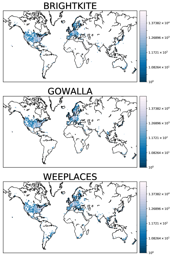
Figure S1: Check-in Maps of Gowalla, BrightKite, and Weeplaces. The colorbar signifies the number of check-ins within a 50km radius, and shows highest coverage in North America and Western Europe

S1.2 Mobility Statistics

The number of unique visited locations, the distribution of jump lengths and the radii of gyration are shown in Figure S2. The latter two quantities are qualitatively identical among the three datasets and consistent with other sources. The distribution of jump lengths resembles a power law distribution, and the tail of the distribution of the radius of gyration closely represents a truncated power law. The distributions of the number of distinct locations illuminate characteristic differences between the datasets. Users of Gowalla are more likely to to visit many locations, while users of BrightKite check-in at very few distinct locations.

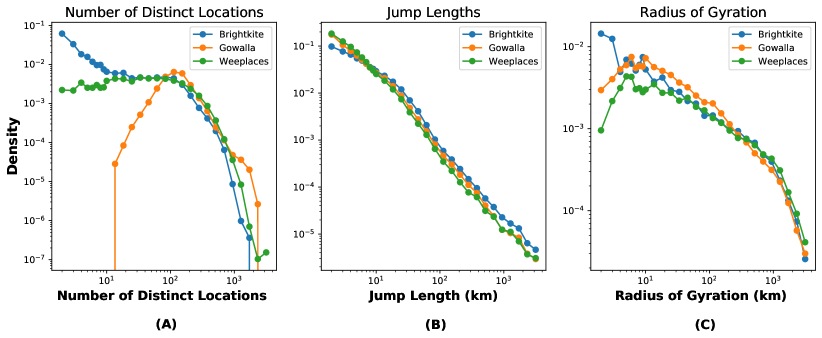
Figure S2: Statistical distributions of selected mobility quantities (A) Distribution of total distinct locations visited by all users in each dataset. (B) Distribution of Jump Lengths of all check-ins of users in the datasets (C) Histogram of Radii of Gyration for all users in the datasets

S1.3 Pre-processing

S1.3.1 Entropy estimator convergence

Because our data is finite and fairly sparse, we need to understand how well the entropy estimators saturate and set thresholds for our data for robustness. We establish a threshold for number of check-ins per user that will yield enough data to analyze the per-user entropy. We heuristically set a threshold of 150 check-ins, plot the entropy rate with respect to a percentage of the ego’s trajectory, and find that the data roughly stabilizes within 50% of the ego’s trajectory.

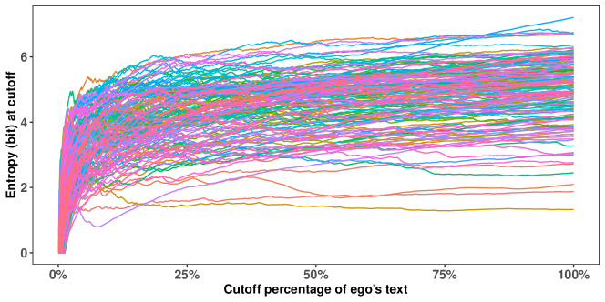
Figure S3: Entropy rate as a function of a percentage of the ego’s trajectory.

S1.3.2 Cross-entropy estimator convergence

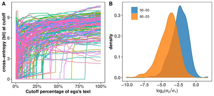
Figure S4: Convergence of Cross Entropy Estimator curve. Shown are the cross entropies of the rank-1 alters for a subset of users (for ease of visualization). (A), The cross entropy of rank-1 alters as a function of a cutoff percentage of the ego’s trajectory (B), The log ratio of the standard deviations of the end and beginning partitions show much lower variability in the latter end of the trajectory, signifying a leveling-off of the cross entropy estimator.

There are some pairs whose cross-entropy varies dramatically over the final portion of the data (Figure S4A). To examine this we plot the cross entropy of rank-1 alters with respect to a cutoff% of their ego’s trajectory. First, we find many alters have check-ins after the last check-in of the ego, leading to a trailing sequence of check-ins that would over-inflate the entropy and do not contribute to the information contained in the ego. Therefore we establish a cutoff of $N_{previous}=150$, meaning there must be at least 150 alter-check-ins before the last check-in of the ego.

We also see from (Figure S4A) that the distribution of check-ins among alters is varied, in that some alters do not have many check-ins at the beginning of the ego’s trajectory, but they satisfy the $N_{previous}>=150$ threshold. To examine the saturation of the entropy and cross-entropy estimators, we partition the data into two portions and compare the variances of the entropy values of the two portions. We use a 50-50 split and an 80-20 split to show how well the cross entropy saturates in the final part of the data compared to the previous. The 80-20 split was chosen based on the 150 check-in minimum, so the final 20% of the data would have at least 30 check-ins for which one could reasonably calculate a variance. The two partitions show that as the number of check-ins increase, the variance in the latter portion relative to the earlier portion is much smaller, indicating that alters with high variability are few as seen in the rapid fall-off in the tail of the distribution. After pre-processing, the summary statistics are shown in LABEL:tab:dataset.

Table S1: The summary of three pre-processed datasets.

Dataset	Total Check-ins	Users	Distinct Placeid
Weeplace	7,049,037	11,533	924,666
BrightKite	3,513,895	6,132	510,308
Gowalla	3,466,392	9,937	850,094

S2 Ego-alter network construction

In each of the LBSNs we use, there exist both a location check-in network and a social network, so we can use the social network to compare against a proxy network. With the check-in network, we can form an artificial social network by assigning connections to users that check in at the same place at the same time. We took a colocation as two users checking in at the same place-id within an hour starting on the hour, eg. 8:00 - 9:00 (The choice of the 1-HR bin for colocation was examined and the details can be found in Section S2.5). We assume that users that co-locate more often contain more predictive information about each other’s whereabouts, so we rank users’ social relationship based on the number of times they co-locate, both in the social relationship and colocation network. Because two people that co-locate are not necessarily social ties, we use the term "ego" to describe users who’s mobility data we are trying to predict by the location history of their "alters" (non-social colocators and social ties).

S2.1 Quality control of colocators

Unlike social relationship, colocation is a theoretical and artificial relationship between two individuals. We find that a user among all datasets reasonably have more colocators than social ties. There are many colocators who are strangers to the user because the two happen to check-in at the same time by accident, eg. a colocator with a single colocation with a user. If user $A$ and $B$ only have one colocation, they are probably strangers to each other and just happen to appear in one place at the same time period by chance. Thus, there is no doubt that $A$ (or $B$) can hardly provide any useful information for $B$ (or $A$) when looking at their previous trajectories. Therefore, we made further quality control by discarding the colocator with only one colocation.

For all users in the datasets, their remaining colocators make up the qualified network and these colocators are called qualified colocators. All colocators used in this paper are qualified colocators, unless indicated otherwise.

S2.2 Contribution control of colocators and social ties

We can use a random algorithm as null model to compare to the information contained in a user’s trajectory. The probability of correct prediction in null model is $1/N_{ego}$ where $N_{ego}$ is the number of unique locations of ego’s historical trajectory. Any useful algorithms have to perform better than a random algorithm and these algorithms should have no fewer than $\log_{2}(N_{ego})$ bits information from the view of information theory. As a consequence, we took further contribution control of both colocators and social ties according to LZ cross-entropy. For any ego, we classified all alters (colocators and social ties) as two groups: "useful" if the ego-alter pair’s LZ cross-entropy is less than $\log_{2}(N_{ego})$, and "useless" otherwise. Additional colocators were found whose sequences had no previous matches to their ego’s sequence at any point in the ego’s trajectory ($w_{b}=0$ in LABEL:eq:CCE). We therefore consider all pairs where the alter’s trajectory contained no previous matches as "useless". After these considerations were made, we considered only the useful alters and discarded the rest.

S2.3 Statistics of constructed network

Table S2: The summary of three filtered datasets. The number of egos who have at least ten alters in both non-social colocation (quality control and contribution control apply) and social (contribution control applies) network. The common networks include the common egos with their respective top ten alters in each network.

Dataset	Non-social colocation network		Social network		Common-Ego networks
	ego	ego-alter pair	ego	ego-alter pair	ego	ego-alter pair
BrightKite	122	2,684	187	4,460	33	330
Gowalla	192	9,332	349	7,681	97	970
Weeplaces	665	21,741	401	8,042	199	1,990

S2.4 Choice of the number of top alters

We would like to choose the highest quality subset of alters among our data. Because we choose colocation as a proxy for social ties, we examine the usefulness of alters based on the number of colocations. We place an additional sub-ranking criteria where alters with the same number of colocations are ranked in increasing order of number of check-ins of the alter. We assume that alters with higher ratios of colocations to number of checkins will provide more information than those with lower ratios. After keeping all useful alters, we look at the average number of colocations per rank of the datasets (Figure S5). All three datasets show that beyond roughly 10 alters, the number of colocations saturates at fewer than around 5 meetups, making the potential influence due to colocation insignificant. Therefore, in our analysis we focused on the contribution from the top ten alters. Cross Entropy distributions of rank-5 (middle) and rank-10 (low) were plotted for both networks for all datasets, and on average the entropies increased with lower rank (Figure S6).

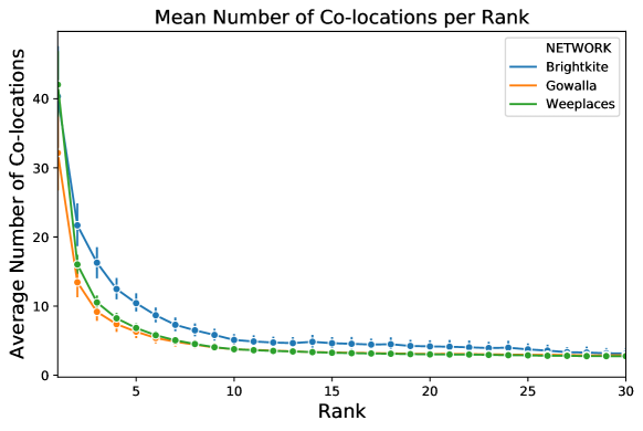
Figure S5: Average number of colocations per rank for all datasets

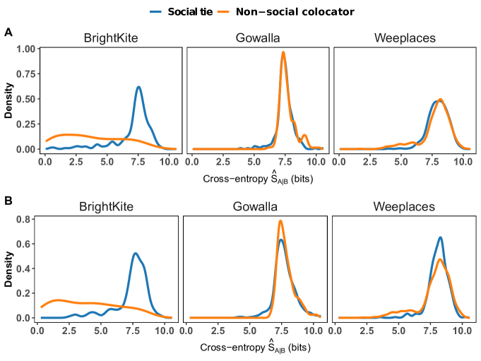
Figure S6: Information contained in alters. (A) Cross-entropy of ego with their rank-5 social tie and rank-5 non-social colocator. (B) Cross-entropy of ego with their rank-10 social tie and rank-10 non-social colocator.

S2.5 Robustness of temporal windows in colocation network construction

The colocation network construction relies on a specified time-resolution, so different time-resolutions would capture different colocators for each ego. To test the robustness of the 1-hour colocation time frame, we compared a 1-hour clock-bin network (colocation on a given day within the interval ($T$:00:00,$T$:59:59), $T\in(0,1,2...,23)$) to a 1-hour sliding-window network (colocation within $\pm 30$ minutes of a check-in of the ego). We consider the 199 egos with at least ten alters in Weeplaces dataset. From Figure S7 we see that within error bars, the colocation networks of different-sized clock bins have statistically similar trends in cumulative cross-predictability. The cumulative predictabilities of ego with increasing number of qualified colocators based on different temporal windows are statistically similar.

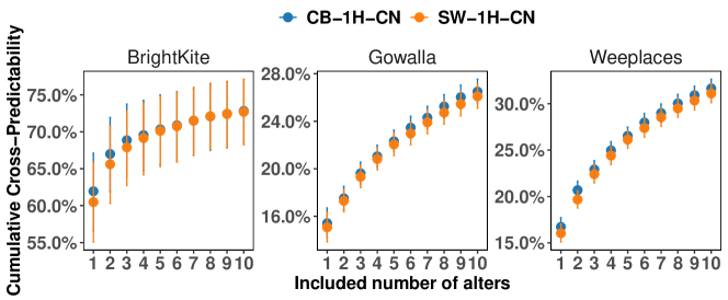
Figure S7: The comparison between choice of 1-hour clock-bin and sliding window in BrightKite, Gowalla, and Weeplaces. Error bars denote $\pm 95\%$ CI.

S3 Information contained in alters

S3.1 Analysis for Brightkite and Gowalla

Figure S8 and Figure S9 show the information-theoretic analysis of Brightkite and Gowalla respectively

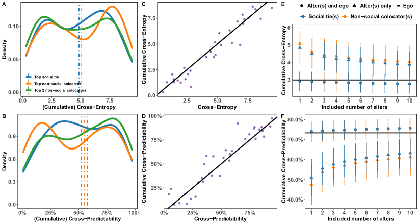
Figure S8: The cross-entropy and predictability provided by social ties and non-social colocators in BrightKite. A Distributions of $\hat{S}_{A|B}$ for the rank-1 social tie (median 4.84 bits), non-social colocator (median 5.03 bits), and $\hat{S}_{A|\mathcal{B}}$ for the top-2 non-social colocators (median 4.90 bits) in B The corresponding $\Pi_{A|B}$ for the social (median 51.94%), and non-social colocators (median 54.84%), and $\Pi_{A|\mathcal{B}}$ for the top-2 non-social colocators (median 57.86%). C $\hat{S}_{A|B}$ encoded in the top-social tie as a function of $\hat{S}_{A|\mathcal{B}}$ for the top-3 non-social colocators. Each point corresponds to a single ego and the solid line denotes $y=x$. D As in panel C but with predictability instead of cross-entropy. E, F $\hat{S}_{A|\mathcal{B}}$ and $\Pi_{A|\mathcal{B}}$ after accumulating the top-ten social alters and non-social colocators. Horizontal lines denote the average entropy ($2.98$ bits) of egos and their self-predictability ($73.33$%). Error bars denote $95\%$ CI.

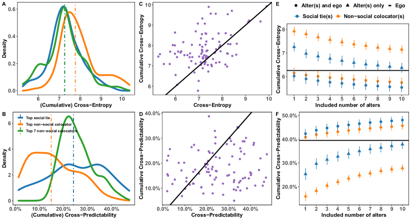
Figure S9: The cross-entropy and predictability provided by social ties and non-social colocators in Gowalla. A Distributions of $\hat{S}_{A|B}$ for the rank-1 social tie (median 7.27 bits), non-social colocator (median 7.77 bits), and $\hat{S}_{A|\mathcal{B}}$ for the top-7 non-social colocators (median 7.26 bits) in B The corresponding $\Pi_{A|B}$ for the social (median 24.14%), and non-social colocators (median 14.92%), and $\Pi_{A|\mathcal{B}}$ for the top-7 non-social colocators (median 24.14%). C $\hat{S}_{A|B}$ encoded in the top-social tie as a function of $\hat{S}_{A|\mathcal{B}}$ for the top-3 non-social colocators. Each point corresponds to a single ego and the solid line denotes $y=x$. D As in panel C but with predictability instead of cross-entropy. E, F $\hat{S}_{A|\mathcal{B}}$ and $\Pi_{A|\mathcal{B}}$ after accumulating the top-ten social alters and non-social colocators. Horizontal lines denote the average entropy ($6.26$ bits) of egos and their self-predictability ($39.49$%). Error bars denote $95\%$ CI.

Figure S10: Homophily in predictability. Scatterplot comparing the predictabilities of egos to their rank-1 alters. All egos are those who have at least both 10 social ties and 10 non-social colocators. The black solid lines in each subplot are $y=x$.

S4 Extrapolating Cross-Predictability

We’ve chosen the top 10 alters in determining the cumulative mobility information flow between the alters’ respective egos. We extrapolate these results by fitting a saturating function to our data, to determine the potential information flow in the limit of infinite alters (or more realistically around 150 alters, the maximum number of social ties a given person can reasonably have). The saturating function used is

$$\Pi(i)=\Pi_{\infty}+\frac{\beta_{0}}{\beta_{1}+i}$$ (S1)

where $i$ is the number of top $i$ included alters. A $\chi^{2}$ minimization of the means and their errors using the BFGS algorithm was used to determine the most likely parameters. A $95\%$ confidence interval of the parameters was determined using a t-test with $10$ alters $-3$ parameters $=7$ degrees of freedom. Results can be found in LABEL:tab:CLN_SRN_CCP_Fits.

Table S3: Parameters for saturating function of the cumulative cross predictability $\Pi(i)$

Dataset &	Brightkite		Gowalla		Weeplaces
Network	Social	Non-Social colocation	Social	Non-social colocation	Social	Non-social colocation
$\Pi_{\infty}$	0.6699 $\pm$ .003313	0.6329 $\pm$ .00504	.4319 $\pm$ 0.005082	.3897 $\pm$ .003186	0.4431 $\pm$ .001039	0.3979 $\pm$ 0.003427
$\beta_{0}$	-0.4629 $\pm$ .03817	-0.2980 $\pm$ .0445	-.7427 $\pm$ .07489	-1.881 $\pm$ .0747	-0.7792 $\pm$ 0.01240	-1.616 $\pm$ .0662
$\beta_{1}$	1.937 $\pm$ .2011	.9096 $\pm$ .25089	3.224 $\pm$ .3323	7.135 $\pm$ .2237	2.083 $\pm$ 0.04045	5.307 $\pm$ .1865

S5 Spatial correlation analysis

We plot the correlation between the cumulative cross-predictability and the CODLR in both types of networks as one progressively adds alters from rank-1 to rank -10 in Figure S11 and Figure S12 for the Weeplaces dataset (571 common egos). While including a single alter yields a Pearson correlation coefficient $R=0.13$ in colocation network and $R=0.27$ in social network, the correlation increases as one progressively adds more alters saturating at $R=0.67$ and $R=0.66$ in colocation network and social network,respectively. We can also the same trend in both BrightKite (See Figure S13 and Figure S14, 122 common egos)and Gowalla ((See Figure S15 and Figure S16), 186 common egos) datasts.

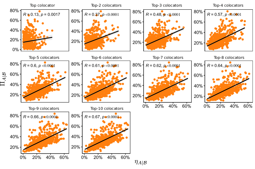
Figure S11: CODLR vs cumulative cross-predictability for non-social ties in Weeplaces. $R$ is Pearson’s correlation coefficient and $p$ is p-value. The solid black lines are linear regression lines.

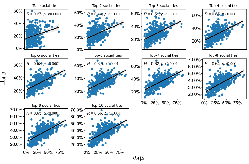
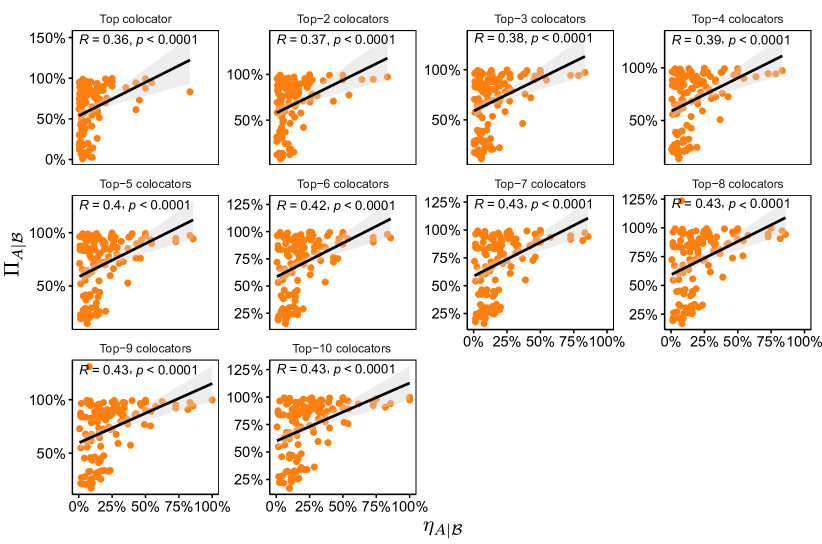
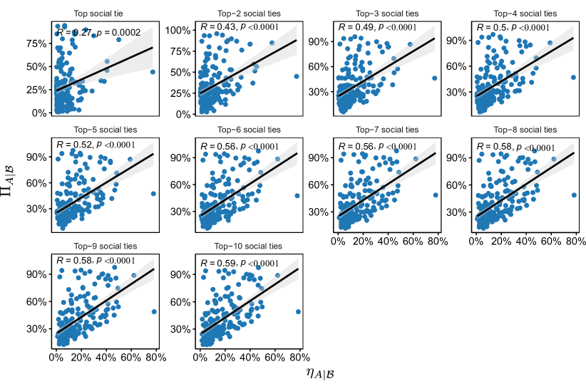
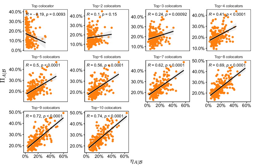
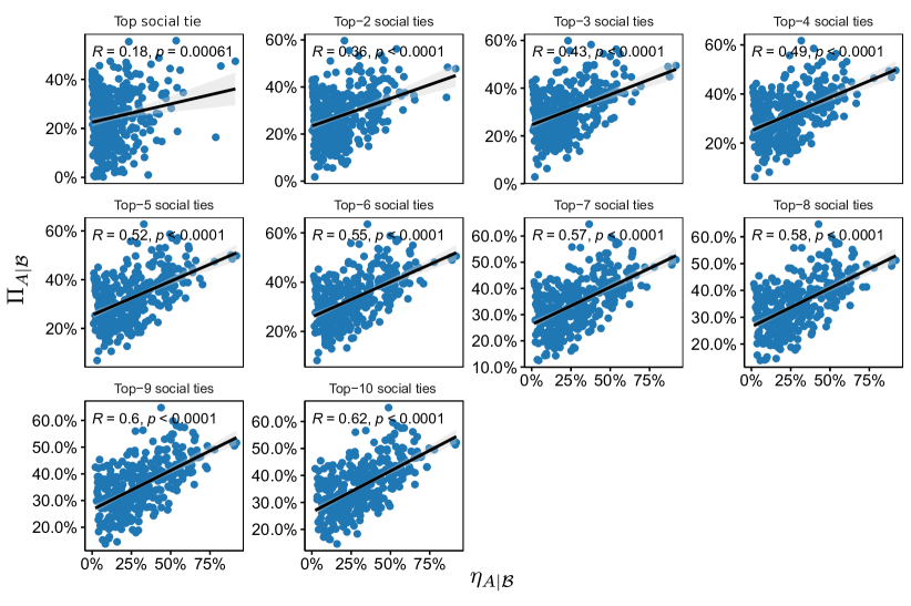
Figure S12: CODLR vs cumulative cross-predictability for social ties in Weeplaces. $R$ is Pearson’s correlation coefficient and $p$ is p-value. The solid black lines are linear regression lines.

Figure S13: CODLR vs cumulative cross-predictability for non-social ties in BrightKite. $R$ is Pearson’s correlation coefficient and $p$ is p-value. The solid black lines are linear regression lines.

Figure S14: CODLR vs cumulative cross-predictability for social ties in BrightKite. $R$ is Pearson’s correlation coefficient and $p$ is p-value. The solid black lines are linear regression lines.

Figure S15: CODLR vs cumulative cross-predictability for non-social ties in Gowalla. $R$ is Pearson’s correlation coefficient and $p$ is p-value. The solid black lines are linear regression lines.

Figure S16: CODLR vs cumulative cross-predictability for social ties in Gowalla. $R$ is Pearson’s correlation coefficient and $p$ is p-value. The solid black lines are linear regression lines.

S6 Time lag effect

To check the similarity in pair-wise connections of the different temporal-lag networks, we compute and Jaccard similarity defined for any two sets $A,B$ as $J(A,B)=\frac{|A\cap B|}{|A\cup B|},$ where $|\cdot|$ is the number of elements in the set. All ego-alter pairs in each type of network are considered the sets $A$ and $B$. The results for selected temporal-lag networks are presented in Figure S17. The $T$Hr-lag networks correspond to sliding windows where an ego check-in at time $t$ colocates with an alter on the interval $(t-T,t-(T-.5))\bigcup((t+(T-.5),t+T)$. This means a $.5$Hr-lag network corresponds to a 1Hr sliding window colocation network with no temporal lag. The ego-alter pairs of all temporal-lag networks are generally different but provide similar trends in cross predictability and in cumulative overlapped distinct locations.

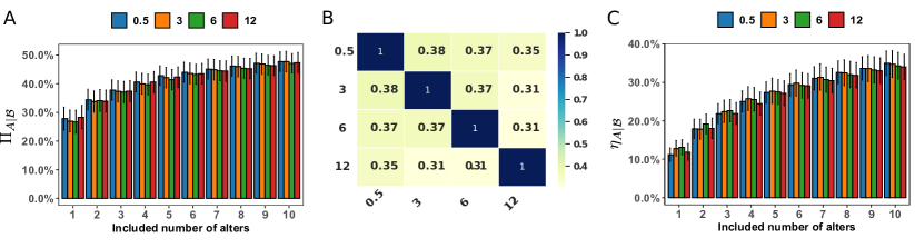
Figure S17: The comparison among the non-social co-located alters within 0.5H, 3H, 6H, 12H one hour sliding windows in Weeplaces dataset. A, (Cumulative) cross-predictability $\Pi_{A|\mathcal{B}}$ VS different included number of alters. B, Global Jaccard Similarity between the the non-social co-located alters within 0.5H, 3H, 6H, 12H one hour sliding windows. C, (Cumulative) overlapped distinct location ratio $\eta_{A|\mathcal{B}}$ VS different included number of alters. Error bars denote mean $\pm 95\%$ CI.