Performance Portable Back-projection Algorithms on CPUs: Agnostic Data Locality and Vectorization Optimizations

Abstract.

Computed Tomography (CT) is a key 3D imaging technology that fundamentally relies on the compute-intense back-projection operation to generate 3D volumes. GPUs are typically used for back-projection in production CT devices. However, with the rise of power-constrained micro-CT devices, and also the emergence of CPUs comparable in performance to GPUs, back-projection for CPUs could become favorable. Unlike GPUs, extracting parallelism for back-projection algorithms on CPUs is complex given that parallelism and locality are not explicitly defined and controlled by the programmer, as is the case when using CUDA for instance. We propose a collection of novel back-projection algorithms that reduce the arithmetic computation, robustly enable vectorization, enforce a regular memory access pattern, and maximize the data locality. We also implement the novel algorithms as efficient back-projection kernels that are performance portable over a wide range of CPUs. Performance evaluation using a variety of CPUs from different vendors and generations demonstrates that our back-projection implementation achieves on average $5.2\times$ speedup over the multi-threaded implementation of the most widely used, and optimized, open library. With a state-of-the-art CPU, we reach performance that rivals top-performing GPUs.

1. Introduction

Computed Tomography (CT) is a key 3D imaging technology used in several fields such as medical analysis, scientific inspection, and non-intrusive testing. Back-projection is a fundamental kernel in most of the image reconstruction algorithms such as FDK (Feldkamp et al., 1984) and iterative reconstruction algorithms (Geyer et al., 2015; Biguri et al., 2016, 2020) that employ the algorithms of forward-projection and back-projection, e.g. MLEM (Shepp and Vardi, 1982; Hudson and Larkin, 1994), EM (Green, 1990), ART (Scarfe and Farman, 2008), and SART (Andersen and Kak, 1984). As a consequence, the back-projection kernel is effectively empowering 100,000s of production CT devices worldwide (Matsumoto et al., 2015). Due to its high computational cost ($\mathcal{O}(N^{4})$ (Scherl et al., 2012; Lu et al., 2016)), back-projection is often the compute bottleneck for reconstructing 3D images. That is specially the case in iterative reconstruction algorithms at which back-projection is called repeatedly (Willemink and Noël, 2019). To meet the critical demands for rapid image reconstruction, in the past decades, a plethora of accelerators were employed to improve the computational performance of back-projection such as linear accelerators (Swindell et al., 1983), ASICs (Wu, 1991), DSPs (Liang et al., 2010), FPGAs (Coric et al., 2002; Xue et al., 2006; Kasik et al., 2012), and distributed systems (Yang et al., 2006; Chen et al., 2019; Wang et al., 2017; Palenstijn et al., 2016; Hidayetoğlu et al., 2020; Gao et al., 2019). Custom processors have been adopted by production CT devices in the earlier generations of CT devices. However, over the last decade, GPUs have increasingly become the main processor used for image reconstruction, due to their programmability and competitive performance (Díez et al., 2007; Cabral et al., 1994; Mueller et al., 2007; Xu and Mueller, 2005; Eklund et al., 2013; Sabne et al., 2017; Rezvani et al., 2007; Zhao et al., 2009; Zinsser and Keck, 2013; Palenstijn et al., 2016; Biguri et al., 2020).

We argue that there are strong reasons for optimizing back-projection kernels for CPUs, despite GPUs being the de facto processor for back-projection over the last decade. First, there is a noticeable trend of portable and lightweight micro-CT devices (Swain and Xue, 2009; Clark and Badea, 2014; Award, 2020; Ying et al., 2017). This further makes CT vendors more sensitive to the cost, power, and space requirements that come along with discrete accelerators. For instance, a state-of-art lineup of industrial micro-CT devices (listed in (Nikon, 2020)) reports power consumption ranging between 225W to 450W. However, low-end GPUs would consume up to 30% of that power budget, and high-end GPUs (i.e. Nvidia’s P100 (Nvidia, 2016) and V100 (Nvidia, 2017)) would consume almost 100% of the power budget of a micro-CT device (Nvidia, 2017). Second, high-performance CPUs with high bandwidth memory can compete with GPUs in raw performance and performance to power. For example, Fujitsu’s A64FX ARM processor (Yoshida, 2018) is equipped with HMB2 memory (Jun et al., 2017) and SVE (Scalable Vector Extension) (Stephens et al., 2017), which pushes the performance to be comparable to the top of line GPUs in a variety of workloads (Sato et al., 2020). Third, integrating accelerators into CT systems increases the system complexity and leads to considerable costs, i.e., hardware and software development. The use of performant CPUs would be preferable since they are a basic component in most CT devices. To conclude, it is crucial to revisit back-projection for CPU, in light of those developments.

We propose novel optimizations at the algorithm-level, and not at the target CPU hardware level. We argue that those carefully designed and novel optimizations at the algorithm level are key to performance portability on a variety of CPUs, having different characteristics. This is in contrast to previous work on CPU back-projection that engineers target-specific optimizations to a single dedicated CPU target (Treibig et al., 2013; Hofmann et al., 2014; Wang et al., 2016a; Karrenberg and Hack, 2012; Lee et al., 2013). It is important to note that, in the context of performance portability, CPUs have much more divergence in characteristics to optimize for, in comparison with GPUs. For instance, the vector width changes from generation to generation (for even the same vendor), while in Nvidia GPUs, the unit of execution (CUDA warp (CUDA, 2020)) maintained the same size in all generations.

We briefly list here the algorithm-level optimizations for back-projection we propose for CPUs. First, effective data locality and regular memory access patterns are critical to improving the efficiency of back-projection kernels. To improve the data locality (Stallings, 2003), we introduce a generic scheme to reschedule the loop ordering, employ data blocking, and change the data layout rearrangement. This is in contrast to other non-portable methods that rely on the gather load intrinsic to deal with the irregular memory access (Treibig et al., 2013). Second, assuring that the SIMD vector units of the CPUs are fully utilized is crucial for performance. Designing back-projection algorithms that are fully vectorizable by compilers, yet being performance portable across CPUs from different vendors is necessary, yet challenging. To assure a loop could vectorize automatically, it is necessary to simplify the iteration space and data accesses such that it can be auto-vectorized by the compiler. We hence gear our optimization techniques to enable the compiler to consistently vectorize the back-projection kernel, regardless of the vector width. Third, back-projection requires high computational resources. It is crucial to improve its performance at the algorithmic level by reducing the arithmetic computation and memory access to the least possible. To that end, we propose a novel double-buffer sub-line algorithm for efficient interpolation at the sub-pixel precision. We also reduce the number of arithmetic operations, by exploiting geometric symmetry, while maintaining contiguous memory access. In addition, we block the sub-line interpolation, to improve the locality without any impediment to the compiler’s capability of automated vectorization.

The contributions in this paper are:

• We propose a collection of novel algorithm-level optimizations for back-projection on CPUs. Our optimizations reduce the computational cost of the projection operations, improve data locality, and consistently enable auto-vectorization.

• We provide a performance portable implementation: a single OpenCL source for all CPUs supporting OpenCL and a single OpenMP source for CPUs that do not support OpenCL (without any trace of processor-specific intrinsics or optimizations).

• We demonstrate that our kernels achieve on average $5.2\times$ speedup over the most widely used and optimized multi-threaded library, on a variety of CPUs from different vendors and generations. Also, we achieve better performance on the Fujitsu A64FX than commonly used open-source CUDA implementation of back-projection on Nvidia V100 Volta GPU (when accounting for unavoidable data movement overhead between host and device).

The rest of this paper is organized as follows: In Section 2, we introduce the background. Section 3 illustrates the proposed algorithms. Section 4 shows the evaluated result. In Section 5, we elaborate on the related work. Finally, Section 6 concludes.

2. Background

In this section, we introduce the details of image reconstruction using the back-projection algorithm and describe the basics of OpenCL for multicore CPUs.

2.1. CT Image reconstruction

This section illustrates the 3D image reconstruction algorithm for Cone-Beam Computed Tomography (CBCT) as presented by Feldkamp et al. (Feldkamp et al., 1984), including the CBCT geometry and back-projection algorithm.

2.1.1. Geometry of CT system

Figure 1 shows the triangular geometry of CBCT system (Scarfe and Farman, 2008). The X-ray source is some form of a microfocus X-ray tube. The Flat Panel Detector (FPD) is a digital radiography imaging sensor, similar to that of digital photography. The distances of the source to the rotation axis (the Z-axis) and FPD are d and D, respectively. The width and height dimensions of the FPD, in the unit of pixel, are nw and nh, respectively. Note that the V-axis of FPD is parallel to Z-axis. The sizes of 3D volume data in a unit of voxel are nx, ny, and nz. The default data layout of volume data is row-major order. As a typical pinhole model (Hartley and Zisserman, 2003), all geometric information can be presented as a matrix of size 3$\times$4 (called projection matrix), which is used for back-projection computation, e.g. projecting a voxel to the plane of FPD as mat in Listing 1. For simplification, we ignore the computation of obtaining the projection matrix via the geometry information. The detailed formulation is available at (Wiesent et al., 2000). Computing the projection, i.e., mapping a 3D point (i, j, k) to the plane of FPD (the UV plane) is shown in Listing 1 (lines 7$\sim$11).

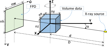
Figure 1. The triangular geometry of a CT system.

Listing 1: Pseudocode of the multi-threaded back-projection implementation adopted by RTK and RabbitCT. The np is the number of projections. The sizes of the 2D projections, 3D volume data, and projection matrices are nh$\times$nw, nz$\times$nx$\times$ny, and 3$\times$4, respectively.

⬇

1void BackProjection(float img[np][nh][nw], float mat[np][3][4], float volume[nz][ny][nx])

2{

3 for (int s = 0; s < np; s++){

4 parallel_for (int k = 0; k < nz; k++){

5 for (int j = 0; j < ny; j++){

6 for (int i = 0; i < nx; i++){

7 float vec[4] = {i,j,k,1.f};//coordinate

8 float z = dot4(mat[s][2], vec); //dot

9 float f = 1.f/z;

10 float x = dot4(mat[s][0], vec)*f; //dot

11 float y = dot4(mat[s][1], vec)*f; //dot

12 float val = Bilinear_Interpolate(img[s], x, y);

13 float w = f*f; //compute weight

14 volume[k][j][i] += val*w;//update

15 } } } } // s, k, j, i

16}

Listing 2: The Bilinear_Interpolate is a bilinear interpolation function. The dot4 is an inner product function and the mix is a built-in common function (e.g. in OpenCL) that returns a linear blend of two variables, where Type can be scalar or vector data types.

⬇

1float Bilinear_Interpolate(float img[nh][nw], float x, float y){

2 int nx = (int)x; //convert to integer

3 int ny = (int)y; //convert to integer

4 //horizontal interpolation using mix

5 float s0 = mix(img[ny ][nx], img[ny ][nx+1], x-nx);

6 float s1 = mix(img[ny+1][nx], img[ny+1][nx+1], x-nx);

7 //vertical interpolation using mix

8 return mix(s0, s1, y-ny);

9}

10float dot4(float v0[4], float v1[4]){//inner product

11 return v0[0]*v1[0]+v0[1]*v1[1]+v0[2]*v1[2]+v0[3];

12}

13Type mix(Type x, Type y, Type a){//linear interpolation

14 return x*((Type)1.f-a) + y*a;

15}

2.1.2. Back-projection

The computational complexity of back-projection is $\mathcal{O}(N^{4})$ (Scherl et al., 2012; Lu et al., 2016). Listing 1 shows the pseudocode of the reference multi-threaded back-projection algorithm as implemented in the widely used RTK library. Note that the pseudocode also matches the multi-threaded implementation of the other most widely used library, RabbitCT (Rohkohl et al., 2009). A parallel loop (line 4) is where the work is divided among the threads to take advantage of the multi-cores of the processor. The inputs to the back projection kernel are: the 2D filtered projections img, the 3D output volume of the filtering computation volume, and the dimensions expressed as (np, nh, nw). Throughout this paper, np refers to the total number of projections, and nb refers to the number of projections in a single batch. More specifically, the projections are equally split into disjoint subsets of projections, where each subset includes a number of projections nb that is used to update the volume data as a batch.

The projection matrix mat is used to project the voxel to the FPD plane. The projected coordinate is written as x and y in lines 10 and 11. The value of z (line 8) is used to derive the projection coordinate, as well as a weighting factor to update the volume data in lines 13$\sim$14. The dot4 operator (line 10), is a customized operator for the inner product as in Listing 2 that is called three times in the most inner loop. As listing 2 shows, a bilinear interpolation function, namely Bilinear_Interpolate, is used to fetch the intensity value of the 2D projections.

2.2. Parallel Computation by OpenCL

OpenCL provides a portable way to take advantage of the SIMD-accelerated processors with a programming approach of single instruction multiple threads. The OpenCL kernels can be compiled dynamically at runtime for the target architecture. OpenCL abstracts an open standard platform for parallel programming and provides a uniform programming interface that is often used to write portable and efficient code for a variety of processors, e.g. CPUs, GPUs, and FPGAs. As an open standard defined by Khronos Group (Wikipedia, 2020a), OpenCL uses a host/device programming model. Programming by OpenCL involves writing host code, often in C/C++, that runs on the host, and a kernel code developed in C, that runs on the device or accelerator. The host codes are often compiled by a general C/C++ compiler (e.g. gcc/g++), and the kernel codes are built at runtime by a target-specific compiler. The computing unit in OpenCL is a work-item. A work-group is a collection of work-items abstracted as a multi-dimensional descriptor named NDRange. Note that the work-items within the same work-group can exchange data using the local memory.

2.3. Terminology

We define the image reconstruction problem and performance metrics in this section. The image reconstruction problem is defined as $nw{\times}nh{\times}np{\Rightarrow}nx{\times}ny{\times}nz$ , where $nw{\times}nh$ and $np$ are the size and number of input projections, respectively. The size of the output volume is defined as $nx{\times}ny{\times}nz$. The performance metric we use is calculated as ${\bf{nx*ny*nz*np*t^{-1}*10^{-9}}}$, where t denotes the run-time in a unit of second. The performance unit of the kernel commonly used in image reconstruction algorithms is GUPS, which stands for Giga Updates per Second.

3. Proposed Back-projection Algorithms

In this section, we discuss a variety of algorithms for back-projection that employ different optimization schemes corresponding to different CPU features, without loss of generality with regard to CPU vendor and generation. The optimization schemes do not interfere with each other and could be combined. We improve the data locality and memory access pattern by transposing projections and volume data. To fully utilize the multi-cores and vector units, we also take advantage of both OpenMP and OpenCL to speed up the back-projection computation. Auto-vectorization can be performed at compile time when using either OpenMP or OpenCL. Without explicit vector instructions, and by carefully writing the code, the OpenCL compiler (OpenCL, 2020) can automatically vectorize instructions by packing multiple work-items together and running them in a SIMD fashion. To improve the data locality and reduce the arithmetic computation, we use a novel sub-line algorithm to cache the interpolated data at sub-pixel precision. More specifically, we improve the data locality of the bilinear interpolation while enabling auto-vectorization.

3.1. Algorithmic Optimizations

This section describes the algorithmic changes we introduce to improve the memory access pattern, reduce arithmetic computation, and expose data-parallel operations. These optimizations apply to both single-core and multicore. Those optimizations at the algorithmic level are key to performance portability.

As shown in Listing 1, the back-projection is driven by voxels, which are updated by their mapped pixels at projections. The values of voxels are independently updated, i.e. an embarrassingly parallel point-wise operation. Hence, the algorithmic optimizations introduced should, in theory, scale with the capacity of computing resources, i.e. number of cores. The following section elaborates on the algorithmic optimizations.

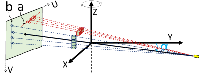
Figure 2. The motivation for transposing projections and volume data. The red and blue voxels are parallel to the X-axis and Z-axis, such that their projection points on the UV plane are lines $\bar{a}$ and $\bar{b}$, respectively. The slope of line $\bar{a}$ changes according to the rotation angle $\alpha$. The line $\bar{b}$ is invariably vertical (namely parallel to both V-axis and Z-axis).

Input : img[nb][nw][nh], mat[nb][3][4], volume[nx][ny][nz], vecIJ $\triangleright$ the pairs of i and j are stored in vecIJ

Output  : volume[nx][ny][nz]

1

2#pragma omp parallel for $\triangleright$ launch multiple threads

3foreach {i, j} $\in$ vecIJ do

4      

5      vec $\leftarrow$ {i, j, 0, 1.f} $\triangleright$ k is independent of X

6      for $s=0$ to $nb-1$ do

7             F[s]$\leftarrow$1.f/dot4(mat[s][2], vec) $\triangleright$ an array of f

8            W[s]$\leftarrow$F[s]*F[s] $\triangleright$ an array of w

9            X[s]$\leftarrow$dot4(mat[s][0], vec)*F[s] $\triangleright$ an array of x

10      

11      for $s=0$ to $nb-1$ do

12             nx$\leftarrow$(int)X[s] $\triangleright$ type convension

13            #pragma omp simd

14            for m=0 to nh-1 do

15                  

16                  sMem[s][m]$\leftarrow$mix(img[s][nh][m], img[s][nh+1][m], X[s]-nX) $\triangleright$ see Figure 3

17            

18      

19      for $k=0$ to $\frac{nz}{2}-1$ do

20            

21            sum$\leftarrow$0 $\triangleright$ register for partial results

22            _sum$\leftarrow$0 $\triangleright$ register for partial results

23            vec[2]$\leftarrow$k; $\triangleright$ update index k

24            #pragma omp simd

25            for $s=0$ to $nb-1$ do

26                   pMem$\leftarrow$sMem[s]

27                  y$\leftarrow$dot4(mat[s][1], vec)*F[s] $\triangleright$ projection comp.

28                  ny$\leftarrow$((int)y $\triangleright$ type conversion

29                  sum$\mathrel{+}=$mix(pMem[ny], pMem[ny+1], y-ny)*W[s]

30                  y$\leftarrow$nh - 1 - y $\triangleright$ geometry symmetry

31                  ny$\leftarrow$(int)y $\triangleright$ type conversion

32                  _sum $\mathrel{+}=$ mix(pMem[ny], pMem[ny+1], y-ny)*W[s]

33            

34            volume[i][j][k] $\mathrel{+}=$ sum $\triangleright$ update volume data

35            volume[i][j][nz-1-k] $\mathrel{+}=$ _sum $\triangleright$ update volume data

36      

Algorithm 1 Proposed back-projection. nb is the batch number. The transposed projection and volume data are presented as img and volume, respectively.

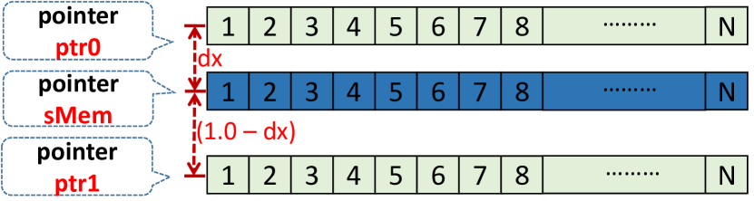
(a) ptr0 and ptr1 are pointers to two neighbouring vertical rows. sMem is a small-sized memory buffer for caching the sub-line values, where 0$\leq$dx$<1$.

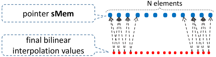
(b) The bilinear interpolation in the horizontal direction. Each output value rely on two neighboring values at the sub-line buffer.

Figure 3. Novel interpolation scheme using sub-line blending. (a) and (b) show vertical and horizontal interpolations.

(a) Vectorize sub-line alg. by C (OpenMP).

(b) Vectorize sub-line alg. by OpenCL.

Figure 4. Implementations of proposed bilinear interpolation scheme. mix is a linear interpolation function in Listing 2.

3.1.1. Towards a Regular Memory Access Pattern

As Listing 1 shows, each voxel is updated by the intensity of projections, according to the projected position at sub-pixel precision using the bilinear interpolation scheme in Listing 2. Figure 2 can be used to visualize the mechanism of bilinear interpolation and also illustrates the optimization of back-projection by transposing the projection and volume data. As shown in the figure, the memory access for the bilinear interpolation along the line $\bar{a}$ is irregular (sloped access to a 2D mesh). Furthermore, the slope of line $\bar{a}$ changes with the rotation angle of $\alpha$. However, the projections of blue voxels (parallel to Z-axis) are in a line $\bar{b}$, which is invariably parallel to V-axis and Z-axis. Therefore, the memory access along line $\bar{b}$ would be regular and unit-strided, if we transpose the projections.

The proposed Algorithm 1 shows the optimization using transposed projections and volume data. More specifically, we optimize the data access pattern by transposing the two-dimensional projections img (input argument). Note that the transposing operation requires marginal time in comparison to the back-projection and can be performed immediately after the pre-processing filtering step, and before the back-projection starts. We also reorganize the loop that iterates the voxels along the Z-axis in the original volume to get unit-strided access over the transposed volume data as the input argument volume shows. More importantly, this transposition operation builds a foundation for further optimizations such as exploiting symmetry and improving the bilinear interpolation scheme to be vectorizable.

3.1.2. Reducing Arithmetic Computation

We reduce the volume of the arithmetic computation by: a) capitalizing on the loop reordering introduced with transposition by moving the loop invariant compute portions outside the inner loop (i.e. hoisting), and b) exploiting geometric symmetry. The data reuse is shown in lines 4$\sim$7 of Algorithm 1. The intermediate variables (namely F, W, and X) are only computed once and their results are shared by the inner loops for further computations, e.g. projection operation, weighting projection intensity, and updating the volume data. Note that the variables F, W, and X contain a small set of values of f, w, and x, respectively (as shown in Listing 1). In this optimization, we exploit the geometric characteristics of back-projection where the values of z and x are constant values when i, j, and the projection matrix (with projection angle $\theta$) are fixed values. That is since the value of z is equal to $d-xcos{\theta}-ycin{\theta}$ (as introduced in (Kak and Slaney, 1988; Lu et al., 2016)), where x and y are coordinates of voxels that correspond to the indexes of i and j. The values of x are also independent of i and j. That is since the projections of voxels are parallel to the V-axis (or Z-axis in Figure 1) at the FPD plane, as introduced in Section 2.1.1.

We also reduce the arithmetic computation by exploiting the geometric symmetry proposed by Zhao et al. (Zhao et al., 2009). As Figure 1 shows, for two voxels that are symmetric to the XY plane, their projections at FPD (namely UV plane) are symmetric to the horizontal centerline of FPD. As line 13 of Algorithm 1 shows, we exploit this symmetry by only performing half of the projection computations for y; the symmetric positions of y can be derived using a single instruction rather than using complex dot and multiply operations.

More specifically, the original number of dot operations is $3*np*nx*ny*nz$, the optimized number of operations is reduced to $np*nx*ny*(1+nz/2)$. Hence, the ratio of reduced computations for dot operations may be written as $({5-2/nz})/{6}{\approx}{5}/{6}$ since $nz\gg 2$ in real-world applications.

Listing 3: A performance-portable OpenCL kernel for back-projection implementing our optimization techniques, e.g. transposing projection and volume data, reordering loops, reusing variables after hoisting, and exploiting geometric symmetry. Constant memory is used to store the projection matrix (see mat), global memory for the projections (see img) and volume data (see volume), where ROWS$\equiv$3, imgDim=(np, nw, nh), volDim=(nx, ny, nz), LM_SIZE=imgDim.x=nh.

⬇

1__kernel void bp_optimized( __constant float4* mat, __global float* img,

2 int3 imgDim, __global float* volume, int3 volDim, __global int2* vecIJ)

3{

4 int k = get_global_id(0); //global index x

5 __local int2 ij; //share index i and j

6 __local float F[nb], X[nb], W[nb], sMem[LM_SIZE];//local mem

7 if (k == 0) ij = vecIJ[get_global_id(1)]; //i and j $\leftarrow$ global index y

8 barrier(CLK_LOCAL_MEM_FENCE); //barrier for local memory

9

10 float4 ijkw = (float4)(ij.x, ij.y, k, 1.f); //vector (i,j,k)

11 if (k < nb) {

12 float z = 1.f / dot((mat + ROWS * k)[2], ijkw);//compute z

13 X[k] = dot((mat + ROWS * k)[0], ijkw)*z; //compute x

14 F[k] = z; //cache z

15 W[k] = z * z; //compute weight

16 }

17 barrier(CLK_LOCAL_MEM_FENCE); //barrier for local memory

18

19 float2 sum = (float2)(0.f, 0.f);

20 for (int s = 0; s < nb; s++, img += imgDim.x∗imgDim.y;, mat += ROWS){

21 int nx = convert_int(X[s]);

22 float dx = X[s] - convert_float(nx);

23 __global float* ptr0 = img + nx * imgDim.x; //see Fig. 3a

24 __global float* ptr1 = ptr0 + imgDim.x; //see Fig. 3a

25 for (int m = k; m < LM_SIZE; m += get_local_size(0))

26 sMem[m] = mix(ptr0[m], ptr1[m], dx); //see Fig. 4

27 barrier(CLK_LOCAL_MEM_FENCE); //barrier for local memory

28

29 float y = dot(mat[1], ijkw)*F[s];

30 float _y = width - 1 - y; //y and _y are symmetric at the vertical line of FPD

31 int2 ny = convert_int2((float2)(y, _y));//float $\rightarrow$ int

32 float2 dy = (float2)(y, _y) - convert_float2(ny);

33 //linear interpolation and update sum as in Fig. 3b

34 sum += mix((float2)(sMem[ny.x], sMem[ny.y]), (float2)(sMem[ny.x+1], sMem[ny.y+1]), dy)*W[s];

35 barrier(CLK_LOCAL_MEM_FENCE); //barrier for local memory

36 }

37 int offset = ij.y*volDim.z*volDim.x + ij.x * volDim.z;

38 volume[offset + k] += sum.x; //update volume

39 volume[offset + volDim.z - 1 - k] += _sum.y; //update volume

40}

3.1.3. Improving locality & Reducing Memory Accesses

We present the details of reducing memory accesses for improving back-projection performance in this section. As discussed by Treibig et al. (Treibig et al., 2013) and Hofmann et al. (Hofmann et al., 2014), back-projection is a bandwidth-limited algorithm and the performance bottleneck is the voxel updates (see line $14$ of Listing 1). In addition to the coalesced access to the memory of volume data proposed by Treibig et al. (Treibig et al., 2013), we improve the algorithm by further reducing the memory accesses to volume data. In the following paragraphs we elaborate.

First, existing multi-threaded implementations (shown in Listing 1) do not split the projections into subsets. This is since the interpolation schemes used in those implementations would reduce the locality if accessing multiple images in the same batch. Contrarily, using batches of images to update the volume is preferable since that would reduce the writes to memory. To use batched projections, one would require a new interpolation scheme to address this issue (more on that in Section 3.1.5).

Second, we reduce memory access to the volume data by using registers to accumulate the partial results (as shown in Algorithm 1). In line 14$\sim$27, we use two registers to accumulate the partial results of voxels for multiple projections in batched processing, then update the volume data by the values accumulated in the registers. Since the cost of accessing registers is negligible with regard to memory access, this batched processing for projections and accumulation of partial results can significantly reduce the number of memory accesses. The original number of elements accessed for the volume data is $4*np*nx*ny*nz$, while after the optimization the number of elements accessed drops to $4*np*nx*ny*nz/nb$. Therefore, in comparison to the baseline implementation, the ratio of memory accesses to the volume data becomes $1/nb$. With a larger value of nb, we can move the bandwidth bottleneck of the memory access from volume data to projections. More specifically, the performance of the proposed algorithm may be bounded by the memory accesses to the projections for the bilinear interpolations. In Section 4, we demonstrate the performance gain of this optimization.

Finally, we also propose a novel bilinear interpolation with vectorization. This optimization can also reduce the memory accesses to some extent as will be discussed in later sections.

3.1.4. Vectorizating Operations

In this section, we present the details of how to enable full utilization of the vector units in the projection operation and interpolation computation in back-projection. Regarding the projection computation (e.g. the computation of x, y, and z in Listing 1), each inner product is performed on two vectors of size $1\times 4$ at single precision. This inner product operation can be perfectly performed by the vector unit, e.g. the built-in function dot is employed for this computation in our OpenCL-based implementation (as will be elaborated later). Note that we benefit from the well-aligned projection matrix of size 3$\times$4 in back-projection algorithms. This is in contrast to other back-projection algorithms, such as in (Lu et al., 2016), at which the projection computation is not vectorizable due to the irregular memory access and compute pattern.

Since we use transposed projections and volume data, the linear interpolation operation can perform the memory accesses in a regular pattern and its computation can also be well vectorized with wide SIMD registers. In Algorithm 1, we can use vector registers for the accumulation of the variables sum and _sum.

In addition, the computation of the second linear interpolation, as in Figure 3b, can be vectorized. More specifically, the memory accesses to update the volume data (lines 26 and 27 in Algorithm 1) can be performed in a vectorized fashion. This vectorized operation can improve the effective memory bandwidth for back-projection, especially in CPUs with High Bandwidth Memory (HBM), e.g. Fujitsu A64FX processor.

3.1.5. A Novel Bilinear Interpolation Scheme

This section discusses our scheme for bilinear interpolation. In linear interpolation, we calculate the target element as a weighted sum from two contributors. In this paper, we use the OpenCL built-in, vectorizable, mix linear blending function (Munshi, 2009). Bilinear interpolation performs a two-dimensional interpolation on a rectilinear grid and thus, it estimates an output element with four known contributors. The conventional back-projection algorithm can not perform the compute pattern in a regular access pattern: bilinear interpolation must be processed on a per-point basis since the data points of the projections are distributed on a sloped line. We capitalize on the transposition of the projections and volume to introduce a bilinear interpolation scheme that blends two lines of pixels in the vertical direction, followed by interpolating in the horizontal direction, where both have a regular access pattern and could be vectorized.

We elaborate on the effect of the proposed scheme on the vectorization of operations: both memory accesses and arithmetic computations. In Figure 3a, the variables ptr0 and ptr1 represent the addresses of two neighboring lines in a transposed projection. We load the data from the memory in a coalesced pattern and thus, the wide SIMD intrinsic can be employed as in the code example in Figure 4b. Figure 4a shows an alternative vectorized OpenMP implementation. It is important to note the regular access pattern for the memory access and arithmetic computations, i.e. loading data from the memory of ptr0/ptr1, storing the result to the memory of sMem, and the linear interpolation operations by the mix function. More specifically, we benefit from this scheme as follows: first, we linearly blend two lines of projections (as ptr0 and ptr1 in Figure 3) into a line of data where all elements in these two lines are only accessed once in a regular pattern. Second, either of the linear interpolations in the horizontal or vertical direction could be easily parallelized. Third, the second linear interpolation can be performed via cache-optimized access of the intermediate memory buffer between the vertical and horizontal steps (sMem in line 12 in Algorithm 1) with better locality and fewer linear interpolation operations.

Table 1. Evaluation environment.

CPU Name	Intel Xeon	Intel Xeon	Intel Xeon	Intel Core	AMD	ThunderX2 (ARM)	Fujitsu (ARM)
	E5-2630 v4	E5-2650 v3	Gold 6140	i7-9700K	EPYC-7452	CN9975	A64FX
Cores	10	10	18	8	32	28	48
Threads/core	2	2	1	1	1	4	1
Frequency	2.2GHz	2.3GHz	2.3GHz	3.6GHz	2.35GHz	1.8GHz	2.2GHz
Sockets	2	2	2	1	2	2	1
GFLOPS (SP)	704	736	2,649	461	2,406	806	6,800
Max bandwidth	137GB/s	137GB/s	250GB/s	42GB/s	205GB/s	159GB/s	1024GB/s
L1d/L1i cache	32K/32K	32K/32K	32K/32K	32K/32K	32K/32K	32K/32K	3M/3M
L2/L3 cache	256K/25M	256K/25M	1M/25M	256K/12M	512K/16M	256K/32M	32M/—
TDP	85W	105W	140W	95W	155W	150W	$\sim$160W

3.2. OpenCL-optimized Back-projection

This section discusses how to take advantage of OpenCL features to implement a performance-portable collection of back-projection kernels based on the optimization techniques we introduced in previous sections.

3.2.1. OpenCL kernel implementation

In Listing 3, we present a performance-portable OpenCL implementation of the back-projection kernel that includes all the discussed optimization techniques in Algorithm 1).

We elaborate on optimizations techniques Listing 3 as follows: (I) we use constant memory (Gaster et al., 2012) to cache the projection matrix mat. The size of each projection matrix is as small as 48B (sizeof(float)*4*3) (II) we pre-pack the indices of $i$ and $j$ in volume data to an array (argument vecIJ to bp_optimized kernel). Each work-group processes all voxels in a single vertical line and thus the indices of i and j can be shared by all work-items in a work-group. We use local memory to share the indices as the variable ij shows. (III) We use local memory to cache the read-only shared data F, X, and W (line 6). Note that the batch number (namely nb) ranges between 1$\sim$32 in our implementations. Hence, the required size of local memory is $sizeof(float)*B*3$, which is within the capacity of local memory. All of these values are only computed once as in lines 11$\sim$16 and reused by all work-items in a work-group. Finally, a barrier is required, line 17, to synchronize all work-items in a work-group. (IV) Using the proposed bilinear scheme (as in Section 3.1.5), we perform the linear interpolation via fast local memory (lines 23$\sim$26). More importantly, we can vectorize the computation as Figure 4 shows. (V) By using the pixel values in local memory (namely sMem), the second linear interpolation can be performed as shown in Figure 3b (line 34). (VI) This kernel also exploits the geometric symmetry to reduce the computation by reusing values computed at the symmetric point, i.e. the value is computed once to be used by the point and its symmetric point (shown as the variables y and _y). We use two-dimensional NDRange to launch this kernel, the local and global parameters may be written as (nz/2, 1) and (nz/2, sizeIJ), respectively. Note that sizeIJ is the number of elements in the array vecIJ. We emphasize the intrinsic that requires the id of work-items in bold font, e.g. get_global_id, get_local_size …, etc. Several built-in functions are used in our implementation such as dot, mix, and convert_T. For more explanations on these built-in functions, the reader can refer to literature as in (Munshi et al., 2011).

Algorithm 2 Prefetching by dual local memory buffers.

Input : $\dots\dots$ $\triangleright$ the input argument are same to Listing 3

1

Output  : volume $\triangleright$ the output volume

2

3__local sMem[2][LM_SIZE] $\triangleright$ declear dual scratchpad memories

4$\text{sMem[0]}\leftarrow img[0]$ $\triangleright$ prefetching by sub-line alg. as in line 26

5$sum\leftarrow 0$ $\triangleright$ declear registers for accumulation

6for $i=0$ to $nb-1$ do

7       if $i+1<B$ then

8             $\text{sMem[(i+1)\%2]}\leftarrow img[i+1]$ $\triangleright$ prefetching without barrier

9       $\text{sum}\leftarrow sMem[i\%2]$ $\triangleright$ accumulate result via subline

10      barrier(CLK_LOCAL_MEM_FENCE) $\triangleright$ barrier work-items

$\text{volume}\leftarrow sum$ $\triangleright$ update volume by batched processing

3.2.2. Prefetching

The use of OpenCL allows us to take advantage of the double buffers technique to overlap the loading operation and computation. As shown in Algorithm 2, we declare dual local memory buffers, which are emphasized in gray color. Hence, we can perform the load operation (line 6) and computation (line 8) using different buffers. However, the allocated memory is doubled, and thus, the available size of processing projections will be limited by the capacity of local memory.

4. Evaluation

In this section, we introduce the evaluation environment, report the results of our experiments, and discuss the advantages and limitations of the proposed algorithms.

4.1. Experiments Setup

Table 1 shows the CPUs we use to evaluate our implementation. We use the same OpenCL implementation on all CPUs, without any customization or optimization to specific targets. For CPUs for which we did not have access to vendor support of OpenCL, we use the same OpenMP implementation, namely the ARM and AMD processors in Table 1.

For the CPUs that use OpenMP library, we employ GCC 9.1.0 (with OpenMP 4.5) for compiling all kernel versions, and ”-O3 -fopenmp -lpthread -std=c++11 -march=native -ftree-vectorize -ftree-slp-vectorize” compilation options. For A64FX processor we use Fujitsu’s compiler FCC 4.0.0 with the compiler options ”-Kopenmp -Kfast -Ksimd=auto -Kassume=memory_bandwidth -O3 -Nlibomp”. On the CPUs that use OpenCL, i.e. Intel CPUs, we use OpenCL SDK-2019.5.345 and runtime 18.1.0 for developing and running OpenCL kernels. All OpenCL kernels are compiled with the compiler options ”-cl-mad-enable -cl-fast-relaxed-math”. Nvidia Tesla P100/V100 GPUs and CUDA 10.0 SDK (CUDA, 2020) are also used for performance comparison.

In Table 2, we list a collection of back-projection kernels that apply the optimizations we proposed in Section 3. We take advantage of both OpenMP and OpenCL to optimize back-projection. The kernel variants of the employed optimization techniques are named ”Transpose”, ”Share”, $\dots$, and ”Prefetching” and they correspond to the optimization techniques discussed in Section 3.1. A collective combination of all optimization techniques (namely symmetry_pf_cl in Table 2) can be found in both Algorithm 1 and Listing 3 for the OpenCL version.

Table 2. Back-projection kernel names and optimizations.

API	Name	Transpose	Share	Symmetry	Subline	LocalMem	Prefetching
	transpose_mp	$\checkmark$
OpenMP	share_mp	$\checkmark$	$\checkmark$
	symmetry_mp	$\checkmark$	$\checkmark$	$\checkmark$
	subline_mp	$\checkmark$	$\checkmark$	$\checkmark$	$\checkmark$
	transpose_cl	$\checkmark$
	share_cl	$\checkmark$	$\checkmark$
	share_lm_cl	$\checkmark$	$\checkmark$			$\checkmark$
OpenCL	symmetry_cl	$\checkmark$	$\checkmark$	$\checkmark$
	symmetry_lm_cl	$\checkmark$	$\checkmark$	$\checkmark$		$\checkmark$
	symmetry_pf_cl	$\checkmark$	$\checkmark$	$\checkmark$		$\checkmark$	$\checkmark$

Table 3. Evaluated image reconstruction problem sizes.

label	Problem	label	Problem
P1	$256^{2}\times 512\Rightarrow 256^{3}$	P7	$1024^{2}\times 512\Rightarrow 256^{3}$
P2	$256^{2}\times 512\Rightarrow 512^{3}$	P8	$1024^{2}\times 512\Rightarrow 512^{3}$
P3	$256^{2}\times 512\Rightarrow 1024^{3}$	P9	$1024^{2}\times 512\Rightarrow 1024^{3}$
P4	$512^{2}\times 512\Rightarrow 256^{3}$
P5	$512^{2}\times 512\Rightarrow 512^{3}$	P10	$1024^{2}\times 512\Rightarrow 1300^{3}$
P6	$512^{2}\times 512\Rightarrow 1024^{3}$		($1300^{3}$ volume is $\sim$8.2GB)

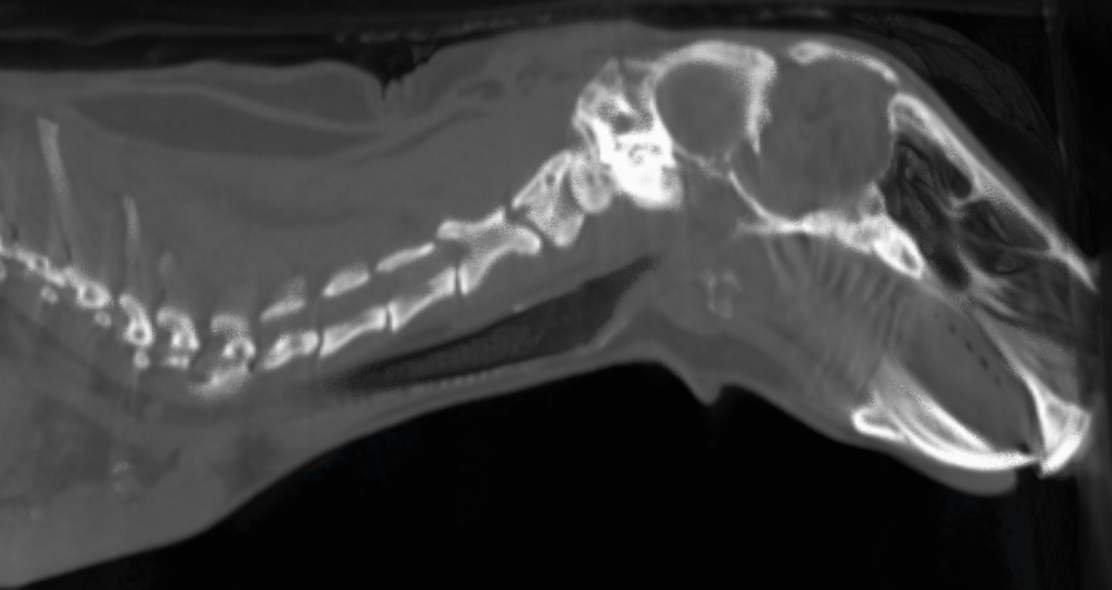
Figure 5. Using our algorithm to reconstruct the volume of the RabbitCT dataset (Rohkohl et al., 2009) ($512\times 512\times 512\Rightarrow 512^{3}$). Rendered by ImageJ 3D Viewer (Rasband et al., 1997).

All evaluations are conducted at single precision. In Table 3, we list the image reconstruction problem sizes, which are labeled as P1, P2,$\dots$, P10. The sizes of the experimental projections include $256^{2}$, $512^{2}$, and $1024^{2}$; the number of projections is fixed as 512; the output problems include $256^{3}$, $512^{3}$, $1024^{3}$, and $1300^{3}$. It is noteworthy that the required memory capacity to store a volume of size $1300^{3}$ is $\sim$8.2 GB.

4.2. Image Reconstruction Results

In Figure 5, we show an example of the generated volume data by our algorithms. The projections are from a real-world CT scanner described in the RabbitCT dataset (Rohkohl et al., 2009). Since the arithmetic computation is independent of the content of projections and volume data, we also use the volume data of RabbitCT to generate a variety of projections as described in Table 3 by a forward-projection tool in the RTK. To verify the output, we compare the reconstructed volume data with the results by RTK library, the Root Mean Square Error (Wikipedia, 2020b) threshold is less than 10e-5. Additionally, we employ the ImageJ (Rasband et al., 1997) (an image processing tool) to render each generated volume data and manually inspect them.

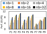
(a) Dual E-2630 CPUs.

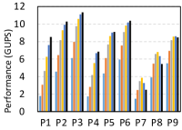
(b) Dual E-2650 CPUs.

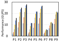
(c) Dual Gold 6140 CPUs.

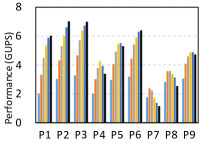
(d) A single i7-9700K CPU.

Figure 6. Performance of top performing kernel (symmetry_pf_cl) with different batch numbers (nb).

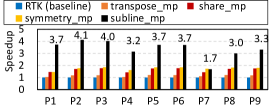
(a) Dual E-2630 CPUs.

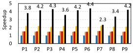
(b) Dual Gold-6140 CPUs.

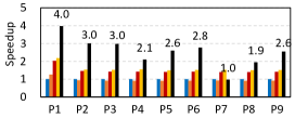
(c) A single i7-9700K CPU.

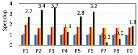
(d) Dual Epyc-7452 CPUs.

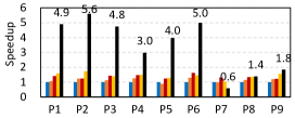
(e) Dual ARM-CN9975 CPUs.

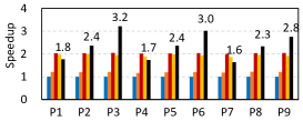
(f) A single A64FX CPU.

Figure 7. Speed up for OpenMP implementation for different levels of optimizations.

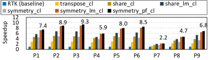
(a) Dual E-2630 CPUs.

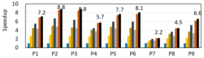
(b) Dual E-2650 CPUs.

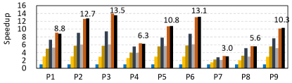
(c) Dual Gold 6140 CPUs.

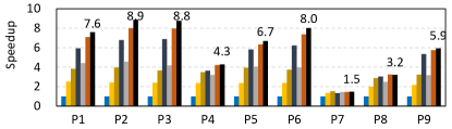
(d) A single i7-9700K CPU.

Figure 8. Speed up for OpenCL implementation (Intel CPUs) at different levels of optimizations.

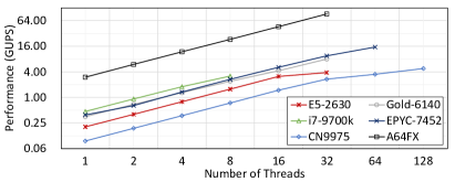
Figure 9. Scaling of the proposed back-projection with the number of threads for problem P5 ($512\times 512\times 512\Rightarrow 512^{3}$).

4.3. Impact of Reducing Memory Accesses

This section discusses the performance impact of reducing memory accesses by batched processing. There are four kernels that reduce the memory accesses, namely subline_mp, share_lm_cl, symmetry_lm_cl, and symmetry_pf_cl (the top performing kernel that includes all optimizations). In Figure 6, we show the performance of symmetry_pf_cl with different configurations values for the batch numbers going: $1,2,4,\dots,32$. The total number of memory accesses to projections (in float32 words) is $N_{memProj}{\approx}4*nx*ny*nz*np$ (four accesses per voxel update by bilinear interpolation). The total number of memory accesses to the volume data is $N_{memVol}=nx*ny*nz*np/{nb}$, as explained in Section 3.1.3. Therefore, the total number of memory accesses are

$$\begin{split}N_{mem}=N_{memProj}+N_{memVol}\approx(4+\frac{1}{nb})*np*nx*ny*nz\end{split}$$

For a given image reconstruction problem, the variables np, nx, ny, and nz are fixed. Consequently, the performance is inversely proportional to $N_{mem}$. When observing the performance in Figure 6, the performance behavior demonstrates this inverse proportional relation to equation $N_{mem}$.

In addition, we observe a performance gain when using a larger batch number for most of the image reconstruction cases. Since the performance of back-projection is bounded by the memory bandwidth, the proposed algorithm benefits from the reduced memory access when batching the projections. To simplify the parameters configuration, in the following experiments we report results for a fixed batch number of 32.

4.4. Performance & Scalability on CPUs

This section reports the performance and scalability of the proposed algorithms. Figure 7 and Figure 8 show the performance of several back-projection kernels on different CPUs and image reconstruction problems as listed in Table 3. The levels of optimization of all evaluated kernels can be found in Table 2. We show speedup over the baseline, which is the multi-threaded and widely used back-projection implementation in the RTK library. The OpenMP-optimized subline_mp and OpenCL-based symmetry_pf_cl achieve the highest performance in most of the cases, due to the collective use of optimizing techniques. The speedup of subline_mp ranges from 0.3 to 5.6 and symmetry_pf_cl ranges from 1.5 to 13.1. Upon investigation, it became clear that this performance differential between OpenMP and OpenCL is due to the higher quality of vectorized code by the OpenCL compiler. Taking the subline kernel as illustrated in Section 3.1.4 for instance, the assembly snippet can be found in Listing 4. The quality of those vectorized codes (AVX2) is competitive to the hand-optimized ones that we tested. To sum up, the portable performance improvement of the proposed algorithms is due to better vectorization, improved data locality, and reduced memory traffic.

Figure 9 shows the scalability of the proposed back-projection algorithm (subline_mp) on several CPUs (listed in Table 1). The number of threads is configured as the power of two and ranges between 1 to 128. The performance on most CPUs scales linearly to the number of cores up to some point where we observe saturation of the memory bus.

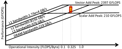
Figure 10. Roofline analysis of symmetry_pf_cl, provided by Intel advisor profiler (Marques et al., 2017; Profilers & Analyzers, 2020) on dual Gold-6140 CPUs. The problem size P1, P2, $\dots$, P9 are shown as yellow dots.

Listing 4: Assembly snippet from symmetry_pf_cl OpenCL kernel with AVX2 vectorization.

⬇

10x177801a62b4 movsxd rdx, edx

20x177801a62b7 vmovups ymm10, ymmword ptr [r8+rdx*4]

30x177801a62bd vmovups ymm11, ymmword ptr [r14+rdx*4]

40x177801a62c3 vsubps ymm11, ymm11, ymm10

50x177801a62c8 vfmadd213ps ymm11, ymm1, ymm10

60x177801a62cd mov rsi, rax

70x177801a62d0 shl rsi, 0xc

80x177801a62d4 add rsi, r11

4.5. Discussion

We show the speedup of several kernels in both Figure 7 and Figure 8 by comparing it with the baseline kernel. We observe the following: (I) OpenCL-based kernels outperform the OpenMP-based kernels due to the difference in the quality of the vectorized codes. The highest speed up among OpenMP-optimized kernels is almost $5.6\times$, in comparison to $13.5\times$ for OpenCL-optimized kernels. (II) Prefetching is effective in improving the performance in several kernels: symmetry_pf_cl (kernel using prefetching) performs better than symmetry_cl (kernel not using prefetching) across different CPUs and image reconstruction problem sizes. The performance gain is noticeable specially in Gold-6140 CPU, likely due to that CPU’s large L2/L3 cache (as listed in Table 1). (III) The bilinear interpolation scheme (in Section 3.1.5) is very effective in improving the performance of back-projection kernels. It is clear that both share_lm_cl and symmetry_lm_cl (kernels using the subline bilinear scheme) perform better than share_cl and symmetry_cl (kernels not using the subline bilinear scheme), respectively. (IV) The optimization techniques such as shared reuse of hoisted variables and exploiting geometry symmetry (illustrated in Section 3.1) contribute to improving the performance of back-projection kernels. The kernels share_cl, share_lm_cl, and symmetry_cl outperform the kernel transposal_cl that only transposes the projection and volume. (V) As shown in Figure 10, we display the Roofline model for the kernel of the top-performing kernel symmetry_pf_cl on dual Gold-6140 CPUs. The optimizations we introduce push the effective achievable bandwidth to be between the bandwidths of L3 and L2 caches.

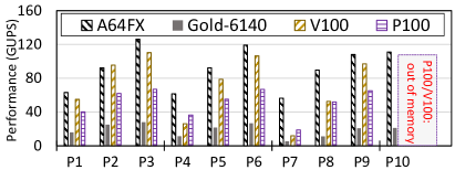
Figure 11. Performance comparison with GPUs at single-precision (end-to-end image reconstruction). Problem P10 can not be solved on P100/V100 GPUs since it exceeds the capacity of device memory. For GPUs, we use the CUDA implementation in the RTK library.

4.5.1. Comparison with GPUs

We demonstrate the competitive performance of our back-projection implementation on the A64FX ARM CPU by comparing it to the high-end Nvidia P100 (Nvidia, 2016) and V100 (Nvidia, 2017) GPUs (see Figure 11). The RTK library implementation for GPUs is used for our comparison. RTK is one of the most widely used open-source library implementations on GPUs, to the author’s knowledge. Our comparison includes the overhead of moving the projections from host memory to device memory and excludes moving the volume back to the CPU. Note that production-level GPU implementations of back-projection (including RTK) do not overlap the computation with moving the projections to the device. That is primarily because overlapping schemes would require complex alterations in the image reconstruction algorithm in addition to being ineffective when scaling the size of projections (i.e. the algorithm cannot function on partial projections).

To conduct a fair comparison, we perform all computations in single precision (without using mixed precision on GPUs or CPUs). Using the A64FX CPU, we can achieve better performance than Tesla P100/V100 GPUs on a wide range of image reconstruction problems. For fairness, we compare our work to RTK’s CUDA implementation since RTK is one of the most used open libraries in both research and industry, though RTK’s performance can be further optimized using the algorithms in (Lu et al., 2016). Note that the implementation in (Lu et al., 2016) is not publicly available. The RTK implementation uses a double buffer method to store volume data (read data from a volume buffer and write the updated value to another buffer). Hence, the maximum capacity of the generated volume must be less than 8 GB. That is because the device memory is limited to 16 GB in P100/V100 GPUs, and a fraction of the device memory is also required to store the projections. It is important to mention that the A64FX can solve the bigger problems such as P10 ($1024^{2}\times 512\Rightarrow 1300^{3}$) in Figure 11, however, the P100/V100 GPUs are restricted by their memory capacities.

To sum up, with the A64FX CPU we reach performance that rivals the top-performing GPUs when accounting for the unavoidable data movement overhead.

5. Related work

Tomographic image reconstruction has been heavily researched in the past years. Target-specific hardware is often adopted to speed up the computation of back-projection. Swindell et al. (Swindell et al., 1983) proposed a linear accelerator to optimize the back-projection for the first generation CT devices three decades ago. Wu et al. (Wu, 1991) used Application-Specific Integrated Circuits (ASIC) to speed up the back-projection algorithm. The authors in (Coric et al., 2002; Xue et al., 2006; Subramanian, 2009; Henry and Chen, 2012) also employed an FPGA to tune the computation of the FDK algorithm. Several authors also use high-level synthesis methods (Coric et al., 2002; Xue et al., 2006; Subramanian, 2009; Henry and Chen, 2012), e.g. OpenCL, to generate the fast back-projection kernels on FPGAs rather than using HDL language. Treibig et al. (Treibig et al., 2013) employed the SIMD instruction set extensions (coded in assembly) to speed up the back-projection computation and achieved outstanding performance on CPUs, e.g. using four Xeon E7-4870 CPU to generate a volume of size $1024^{3}$ and achieve the performance of $12$ GUPS. Notably, such performance is less than a quarter of the peak performance on Intel CPUs. Furthermore, Treibig et al. took advantage of the gather load intrinsic to alleviate the pressure of memory traffic on accessing projections (e.g. access along line $\bar{a}$ in Figure 2). However, the performance of the optimized kernel was still bounded by the memory accesses to update the volume data. Unlike their method, we can fully vectorize the back-projection and reduce the memory access for projection and volume data. In (Hofmann et al., 2014), Johannes et al. optimized the RabbitCT benchmark on the Intel Xeon Phi accelerator. Using a fixed-point DSP (Digital Signal Processor) platform, Liang et al. presented an optimized implementation of FDK and achieved state-of-art balance in cost and power consumption (Liang et al., 2010). On several hardware accelerator platforms such as CPUs, GPGPUs, and Intel Xeon Phi, Serrano et al. (Serrano et al., 2014) proposed a parallelized FDK implementation.

Xiao et al. (Wang et al., 2016b) proposed a super-voxel technique to improve the data locality of the MBIR algorithm. However, super-voxels were restricted for parallel-beam based CT. Mert et al. (Hidayetoğlu et al., 2020) optimized an iterative image reconstruction algorithm and achieved petaflops performance on Summit supercomputer for parallel-beam CT systems, yet their solution is difficult to be applied to the current generation of CT devices (namely Cone-beam CT). In this work, we target Cone-beam datasets ($7^{t}h$ generation CT) for which voxel-based back-projection is required. Lu et al. (Lu et al., 2016) proposed a highly optimized back-projection algorithm for out-of-core computations. Their implementation is more specific for CUDA, e.g. using texture memory. Furthermore, the projection computation in our algorithms is fully different from their approach, e.g. we use the 3$\times$4 projection matrix shown in Listing 1.

RTK library (the baseline of this work) is a widely used library for image reconstruction and provides implementations of back-projection kernels for both CPU and GPU architectures. Due to the complexity of overlapping schemes in back-projection, the unavoidable overhead of data movement between host and device may degrade the performance. Furthermore, the GPU memory is limited and thus, volume decomposition techniques are required to go out-of-core (Lu et al., 2016; Biguri et al., 2020).

6. Conclusion

We revisit the role of CPUs in image reconstruction, motivated by the considerations of cost, power, and space requirements. To use CPUs for compute-intensive medical image processing applications, this paper proposes performance portable back-projection algorithms and demonstrates the performance/scaling on a wide range of multicore processors. Our implementations benefit from the agnostic vectorization, improved memory access pattern, and reduced arithmetic computations. We also propose a bilinear interpolation algorithm to cache the sub-line values of projections for reducing the memory access and the arithmetic computations. Our results show that the proposed back-projection can achieve, on average, 5.2$\times$ speedup over the multi-threaded implementation of the most widely used library, on a wide variety of CPUs. We demonstrate the capability of using an ARM CPU (A64FX) to outperform high-end GPUs in the domain of CT, which is traditionally driven by GPUs.

References

- (1)
- Andersen and Kak (1984) Anders H Andersen and Avinash C Kak. 1984. Simultaneous algebraic reconstruction technique (SART): a superior implementation of the ART algorithm. Ultrasonic imaging 6, 1 (1984), 81–94.
- Award (2020) Good Design Award. 2020. Compact CT (computed tomography) device. https://www.g-mark.org/award/describe/45487?locale=en. [Online; accessed 20-Jan-2021].
- Biguri et al. (2016) Ander Biguri, Manjit Dosanjh, Steven Hancock, and Manuchehr Soleimani. 2016. TIGRE: a MATLAB-GPU toolbox for CBCT image reconstruction. Biomedical Physics & Engineering Express 2, 5 (sep 2016), 055010. https://doi.org/10.1088/2057-1976/2/5/055010
- Biguri et al. (2020) Ander Biguri, Reuben Lindroos, Robert Bryll, Hossein Towsyfyan, Hans Deyhle, Ibrahim El khalil Harrane, Richard Boardman, Mark Mavrogordato, Manjit Dosanjh, Steven Hancock, and Thomas Blumensath. 2020. Arbitrarily large tomography with iterative algorithms on multiple GPUs using the TIGRE toolbox. J. Parallel and Distrib. Comput. 146 (2020), 52 – 63. https://doi.org/10.1016/j.jpdc.2020.07.004
- Cabral et al. (1994) Brian Cabral, Nancy Cam, and Jim Foran. 1994. Accelerated volume rendering and tomographic reconstruction using texture mapping hardware. In Proceedings of the 1994 symposium on Volume visualization. 91–98.
- Chen et al. (2019) Peng Chen, Mohamed Wahib, Shinichiro Takizawa, Ryousei Takano, and Satoshi Matsuoka. 2019. iFDK: A Scalable Framework for Instant High-Resolution Image Reconstruction. In Proceedings of the International Conference for High Performance Computing, Networking, Storage and Analysis (SC ’19). Association for Computing Machinery, New York, NY, USA, Article 84, 24 pages. https://doi.org/10.1145/3295500.3356163
- Clark and Badea (2014) DP Clark and CT Badea. 2014. Micro-CT of rodents: state-of-the-art and future perspectives. Physica medica 30, 6 (2014), 619–634.
- Coric et al. (2002) Srdjan Coric, Miriam Leeser, Eric Miller, and Marc Trepanier. 2002. Parallel-beam backprojection: an FPGA implementation optimized for medical imaging. In Proceedings of the 2002 ACM/SIGDA tenth international symposium on Field-programmable gate arrays. ACM, 217–226.
- CUDA (2020) NVIDIA CUDA. 2020. CUDA Toolkit Documentation. NVIDIA Developer Zone. http://docs.nvidia.com/cuda/index.html (2020).
- Díez et al. (2007) Daniel Castaño Díez, Hannes Mueller, and Achilleas S Frangakis. 2007. Implementation and performance evaluation of reconstruction algorithms on graphics processors. Journal of Structural Biology 157, 1 (2007), 288–295.
- Eklund et al. (2013) Anders Eklund, Paul Dufort, Daniel Forsberg, and Stephen M. LaConte. 2013. Medical image processing on the GPU – Past, present and future. Medical Image Analysis 17, 8 (2013), 1073 – 1094. https://doi.org/10.1016/j.media.2013.05.008
- Feldkamp et al. (1984) LA Feldkamp, LC Davis, and JW Kress. 1984. Practical cone-beam algorithm. JOSA A 1, 6 (1984), 612–619.
- Gao et al. (2019) Yushan Gao, Ander Biguri, and Thomas Blumensath. 2019. Block stochastic gradient descent for large-scale tomographic reconstruction in a parallel network. CoRR abs/1903.11874 (2019). arXiv:1903.11874 http://arxiv.org/abs/1903.11874
- Gaster et al. (2012) Benedict Gaster, Lee Howes, David R Kaeli, Perhaad Mistry, and Dana Schaa. 2012. Heterogeneous computing with openCL: revised openCL 1. Newnes.
- Geyer et al. (2015) Lucas L Geyer, U Joseph Schoepf, Felix G Meinel, John W Nance Jr, Gorka Bastarrika, Jonathon A Leipsic, Narinder S Paul, Marco Rengo, Andrea Laghi, and Carlo N De Cecco. 2015. State of the art: iterative CT reconstruction techniques. Radiology 276, 2 (2015), 339–357.
- Green (1990) Peter J Green. 1990. Bayesian reconstructions from emission tomography data using a modified EM algorithm. IEEE transactions on medical imaging 9, 1 (1990), 84–93.
- Hartley and Zisserman (2003) Richard Hartley and Andrew Zisserman. 2003. Multiple view geometry in computer vision. Cambridge university press.
- Henry and Chen (2012) I Henry and Ming Chen. 2012. An FPGA Architecture for Real-Time 3-D Tomographic Reconstruction. Ph.D. Dissertation. University of California, Los Angeles.
- Hidayetoğlu et al. (2020) Mert Hidayetoğlu, Tekin Bicer, Simon Garcia de Gonzalo, Bin Ren, Vincent De Andrade, Doga Gursoy, Raj Kettimuthu, Ian T. Foster, and Wen-mei W. Hwu. 2020. Petascale XCT: 3D Image Reconstruction with Hierarchical Communications on Multi-GPU Nodes. In Proceedings of the International Conference for High Performance Computing, Networking, Storage and Analysis (SC ’20). IEEE Press, Article 37, 13 pages.
- Hofmann et al. (2014) Johannes Hofmann, Jan Treibig, Georg Hager, and Gerhard Wellein. 2014. Performance engineering for a medical imaging application on the Intel Xeon Phi accelerator. In ARCS 2014; 2014 Workshop Proceedings on Architecture of Computing Systems. VDE, 1–8.
- Hudson and Larkin (1994) H Malcolm Hudson and Richard S Larkin. 1994. Accelerated image reconstruction using ordered subsets of projection data. IEEE transactions on medical imaging 13, 4 (1994), 601–609.
- Jun et al. (2017) Hongshin Jun, Jinhee Cho, Kangseol Lee, Ho-Young Son, Kwiwook Kim, Hanho Jin, and Keith Kim. 2017. Hbm (high bandwidth memory) dram technology and architecture. In 2017 IEEE International Memory Workshop (IMW). IEEE, 1–4.
- Kak and Slaney (1988) Avinash C.. Kak and Malcolm Slaney. 1988. Principles of computerized tomographic imaging. IEEE press New York.
- Karrenberg and Hack (2012) Ralf Karrenberg and Sebastian Hack. 2012. Improving performance of OpenCL on CPUs. In International Conference on Compiler Construction. Springer, 1–20.
- Kasik et al. (2012) Vladimir Kasik, Martin Cerny, Marek Penhaker, Václav Snášel, Vilem Novak, and Radka Pustkova. 2012. Advanced CT and MR image processing with FPGA. In International Conference on Intelligent Data Engineering and Automated Learning. Springer, 787–793.
- Lee et al. (2013) Joo Hwan Lee, Kaushik Patel, Nimit Nigania, Hyojong Kim, and Hyesoon Kim. 2013. OpenCL performance evaluation on modern multi core CPUs. In 2013 IEEE International Symposium on Parallel & Distributed Processing, Workshops and Phd Forum. IEEE, 1177–1185.
- Liang et al. (2010) Wenxuan Liang, Hui Zhang, and Guangshu Hu. 2010. Optimized implementation of the FDK algorithm on one digital signal processor. Tsinghua Science and Technology 15, 1 (2010), 108–113.
- Lu et al. (2016) Yuechao Lu, Fumihiko Ino, and Kenichi Hagihara. 2016. Cache-aware GPU optimization for out-of-core cone beam CT reconstruction of high-resolution volumes. IEICE TRANSACTIONS on Information and Systems 99, 12 (2016), 3060–3071.
- Marques et al. (2017) Diogo Marques, Helder Duarte, Aleksandar Ilic, Leonel Sousa, Roman Belenov, Philippe Thierry, and Zakhar A Matveev. 2017. Performance analysis with cache-aware roofline model in intel advisor. In 2017 International Conference on High Performance Computing & Simulation (HPCS). IEEE, 898–907.
- Matsumoto et al. (2015) Masatoshi Matsumoto, Soichi Koike, Saori Kashima, and Kazuo Awai. 2015. Geographic Distribution of CT, MRI and PET Devices in Japan: A Longitudinal Analysis Based on National Census Data. PLOS ONE 10, 5 (05 2015), 1–12. https://doi.org/10.1371/journal.pone.0126036
- Mueller et al. (2007) Klaus Mueller, F Xu, and N Neophytou. 2007. Why do GPUs work so well for acceleration of CT? SPIE Electronic Imaging07 (2007). http://cvc.cs.stonybrook.edu/Publications/2007/MXN07a
- Munshi (2009) Aaftab Munshi. 2009. The opencl specification. In Hot Chips 21 Symposium (HCS), 2009 IEEE. IEEE, 1–314.
- Munshi et al. (2011) Aaftab Munshi, Benedict Gaster, Timothy G Mattson, and Dan Ginsburg. 2011. OpenCL programming guide. Pearson Education.
- Nikon (2020) Nikon. 2020. Computed Tomography Products. https://www.nikonmetrology.com/en-gb/products/x-ray-and-ct-inspection/computed-tomography.
- Nvidia (2016) Nvidia. 2016. NVIDIA Tesla P100. GP100 Pascal Whitepaper. https://images.nvidia.com/content/pdf/tesla/whitepaper/pascal-architecture-whitepaper.pdf (2016).
- Nvidia (2017) Nvidia. 2017. NVIDIA TESLA V100 GPU ARCHITECTURE. Technical whitepaper. https://images.nvidia.com/content/technologies/volta/pdf/tesla-volta-v100-datasheet-letter-fnl-web.pdf (2017).
- OpenCL (2020) Intel OpenCL. 2020. Intel SDK For OpenCL Applications. https://software.intel.com/content/www/us/en/develop/tools/opencl-sdk.html [Online; accessed 20-Jan-2021].
- Palenstijn et al. (2016) Willem Jan Palenstijn, Jeroen Bédorf, Jan Sijbers, and K Joost Batenburg. 2016. A distributed ASTRA toolbox. Advanced structural and chemical imaging 2, 1 (2016), 1–13.
- Profilers & Analyzers (2020) Intel Profilers & Analyzers. 2020. Intel Advisor. https://software.intel.com/content/www/us/en/develop/tools/advisor.html [Online; accessed 20-Jan-2021].
- Rasband et al. (1997) Wayne S Rasband et al. 1997. ImageJ. http://www.worldlibrary.in/articles/eng/ImageJ. [Online; accessed 20-Jan-2021].
- Rezvani et al. (2007) N Rezvani, D Aruliah, K Jackson, D Moseley, and J Siewerdsen. 2007. SU-FF-I-16: OSCaR: An open-source cone-beam CT reconstruction tool for imaging research. Medical Physics 34, 6Part2 (2007), 2341–2341.
- Rohkohl et al. (2009) Christopher Rohkohl, Benjamin Keck, HG Hofmann, and Joachim Hornegger. 2009. RabbitCT—an open platform for benchmarking 3D cone-beam reconstruction algorithms. Medical Physics 36, 9Part1 (2009), 3940–3944.
- Sabne et al. (2017) Amit Sabne, Xiao Wang, Sherman J Kisner, Charles A Bouman, Anand Raghunathan, and Samuel P Midkiff. 2017. Model-based iterative CT image reconstruction on GPUs. ACM SIGPLAN Notices 52, 8 (2017), 207–220.
- Sato et al. (2020) Mitsuhisa Sato, Yutaka Ishikawa, Hirofumi Tomita, Yuetsu Kodama, Tetsuya Odajima, Miwako Tsuji, Hisashi Yashiro, Masaki Aoki, Naoyuki Shida, Ikuo Miyoshi, Kouichi Hirai, Atsushi Furuya, Akira Asato, Kuniki Morita, and Toshiyuki Shimizu. 2020. Co-Design for A64FX Manycore Processor and ”Fugaku”. In Proceedings of the International Conference for High Performance Computing, Networking, Storage and Analysis (SC ’20). IEEE Press, Article 47, 15 pages.
- Scarfe and Farman (2008) William C Scarfe and Allan G Farman. 2008. What is cone-beam CT and how does it work? Dental Clinics of North America 52, 4 (2008), 707–730.
- Scherl et al. (2012) Holger Scherl, Markus Kowarschik, Hannes G Hofmann, Benjamin Keck, and Joachim Hornegger. 2012. Evaluation of state-of-the-art hardware architectures for fast cone-beam CT reconstruction. Parallel computing 38, 3 (2012), 111–124.
- Serrano et al. (2014) Estefania Serrano, Guzman Bermejo, Javier Garcia Blas, and Jesus Carretero. 2014. High-performance X-ray tomography reconstruction algorithm based on heterogeneous accelerated computing systems. In Cluster Computing (CLUSTER), 2014 IEEE International Conference on. IEEE, 331–338.
- Shepp and Vardi (1982) Lawrence A Shepp and Yehuda Vardi. 1982. Maximum likelihood reconstruction for emission tomography. IEEE transactions on medical imaging 1, 2 (1982), 113–122.
- Stallings (2003) William Stallings. 2003. Computer organization and architecture: designing for performance. Pearson Education India.
- Stephens et al. (2017) Nigel Stephens, Stuart Biles, Matthias Boettcher, Jacob Eapen, Mbou Eyole, Giacomo Gabrielli, Matt Horsnell, Grigorios Magklis, Alejandro Martinez, Nathanael Premillieu, et al. 2017. The ARM scalable vector extension. IEEE Micro 37, 2 (2017), 26–39.
- Subramanian (2009) Nikhil Subramanian. 2009. A C-to-FPGA solution for accelerating tomographic reconstruction. Ph.D. Dissertation. University of Washington.
- Swain and Xue (2009) Michael V Swain and Jing Xue. 2009. State of the art of Micro-CT applications in dental research. International journal of oral science 1, 4 (2009), 177–188.
- Swindell et al. (1983) William Swindell, Robert G Simpson, James R Oleson, Ching-Tai Chen, and Elmer A Grubbs. 1983. Computed tomography with a linear accelerator with radiotherapy applications. Medical Physics 10, 4 (1983), 416–420.
- Treibig et al. (2013) Jan Treibig, Georg Hager, Hannes G Hofmann, Joachim Hornegger, and Gerhard Wellein. 2013. Pushing the limits for medical image reconstruction on recent standard multicore processors. The International Journal of High Performance Computing Applications 27, 2 (2013), 162–177.
- Wang et al. (2016a) Xiao Wang, Amit Sabne, Sherman J. Kisner, Anand Raghunathan, Charles A. Bouman, and Samuel P. Midkiff. 2016a. High Performance Model-Based Image Reconstruction. 21st ACM SIGPLAN Symposium on Principles and Practice of Parallel Programming (PPoPP’16) (2016), 2:1–2:12. https://github.com/HPImaging/sv-mbirct
- Wang et al. (2016b) Xiao Wang, Amit Sabne, Sherman J. Kisner, Anand Raghunathan, Charles A. Bouman, and Samuel P. Midkiff. 2016b. High Performance Model-Based Image Reconstruction. 21st ACM SIGPLAN Symposium on Principles and Practice of Parallel Programming (PPoPP’16) (2016), 2:1–2:12. https://github.com/HPImaging/sv-mbirct
- Wang et al. (2017) Xiao Wang, Amit Sabne, Putt Sakdhnagool, Sherman J Kisner, Charles A Bouman, and Samuel P Midkiff. 2017. Massively parallel 3D image reconstruction. In Proceedings of the International Conference for High Performance Computing, Networking, Storage and Analysis. 1–12.
- Wiesent et al. (2000) Karl Wiesent, Karl Barth, Nassir Navab, Peter Durlak, Thomas Brunner, Oliver Schuetz, and Wolfgang Seissler. 2000. Enhanced 3-D-reconstruction algorithm for C-arm systems suitable for interventional procedures. IEEE transactions on medical imaging 19, 5 (2000), 391–403.
- Wikipedia (2020a) Wikipedia. 2020a. Khronos Group — Wikipedia, The Free Encyclopedia. http://en.wikipedia.org/w/index.php?title=Khronos%20Group&oldid=952509717. [Online; accessed 20-Jan-2021].
- Wikipedia (2020b) Wikipedia. 2020b. Root-mean-square deviation — Wikipedia, The Free Encyclopedia. http://en.wikipedia.org/w/index.php?title=Root-mean-square%20deviation&oldid=941256353. [Online; accessed 20-Jan-2021].
- Willemink and Noël (2019) Martin J Willemink and Peter B Noël. 2019. The evolution of image reconstruction for CT—from filtered back projection to artificial intelligence. European radiology 29, 5 (2019), 2185–2195.
- Wu (1991) Michael A Wu. 1991. ASIC applications in computed tomography systems. In ASIC Conference and Exhibit, 1991. Proceedings., Fourth Annual IEEE International. IEEE, P1–3.
- Xu and Mueller (2005) Fang Xu and Klaus Mueller. 2005. Accelerating popular tomographic reconstruction algorithms on commodity PC graphics hardware. IEEE Transactions on nuclear science 52, 3 (2005), 654–663.
- Xue et al. (2006) Xinwei Xue, Arvi Cheryauka, and David Tubbs. 2006. Acceleration of fluoro-CT reconstruction for a mobile C-Arm on GPU and FPGA hardware: a simulation study. In Medical Imaging 2006: Physics of Medical Imaging, Vol. 6142. International Society for Optics and Photonics, 61424L.
- Yang et al. (2006) Jiansheng Yang, Xiaohu Guo, Qiang Kong, Tie Zhou, and Ming Jiang. 2006. Parallel implementation of Katsevich’s FBP algorithm. International journal of biomedical imaging 2006 (2006).
- Ying et al. (2017) Xiaoyou Ying, Norman J Barlow, and Maureen H Feuston. 2017. Micro–Computed Tomography and Volumetric Imaging in Developmental Toxicology. In Reproductive and Developmental Toxicology. Elsevier, 1183–1205.
- Yoshida (2018) Toshio Yoshida. 2018. Fujitsu high performance CPU for the Post-K Computer. In Hot Chips, Vol. 30.
- Zhao et al. (2009) Xing Zhao, Jing-jing Hu, and Peng Zhang. 2009. GPU-based 3D cone-beam CT image reconstruction for large data volume. Journal of Biomedical Imaging 2009 (2009), 8.
- Zinsser and Keck (2013) Timo Zinsser and Benjamin Keck. 2013. Systematic performance optimization of cone-beam back-projection on the Kepler architecture. Proceedings of the 12th Fully Three-Dimensional Image Reconstruction in Radiology and Nuclear Medicine (2013), 225–228.