Quasinormal Modes of Black Holes with Non-Linear-Electrodynamic sources in Rastall Gravity

Abstract

One of the notable modifications of General Relativity (GR) is the Rastall gravity. We have studied the quasinormal modes of black holes in Rastall gravity in presence of non-linear electrodynamic sources. Here the impacts of cosmological field, dust field, phantom field, quintessence field and radiation field on the quasinormal modes in presence of electrodynamic sources have been investigated. Apart from this, we have also checked the dependency of quasinormal modes with the Rastall parameter $\lambda$, black hole structural constant $N_{s}$ and charge of the black hole $Q$. The study shows that the quasinormal modes corresponding to the black hole with non-linear electrodynamic sources show significant deviations from a general charged black hole in Rastall gravity under certain conditions. Further, the behaviour of black holes and hence the quasinormal modes depend on the type of surrounding field considered.

I Introduction

The existence of black holes and Gravitational Waves (GWs) are two most significant predictions of General Relativity (GR). The binary black hole systems predicted by the ground based Laser Interferometer Gravitational Wave Observatory (LIGO), and Variability of Solar Irradiance and Gravity Oscillations (Virgo) detector systems stand as a valid evidence for the viability of GR. The direct detection of GWs by LIGO and Virgo provided us a new way to test different theories of gravity including GR. GR had already passed experimental tests in the weak field regimes and moderately relativistic regimes such as in the solar system tests will2014 and in binary pulsars hulse1975 ; damour1992 . The recent detections of GWs by the LIGO and Virgo have also established the viability of GR in the highly relativistic strong gravity regime connected to binary black holes. Nonetheless GR has two main issues or drawbacks. Firstly, in the high energy regime the theory is not re-normalizable stelle and secondly, in the infrared regime the theory deviates largely from the experimental observations, especially the observations of accelerated expansion and hidden matter content of the universe are outside of the predictions of GR Riess1998 ; Perlmutter1999 ; Bahcall1999 . Due to these issues, extensions of GR known as Modified Theories of Gravity (MTGs) are introduced. Basically, the extensions of GR are of two types, in one type the spacetime geometry is modified and in the other type, the modifications are done in the matter-energy sector. The simplest extension of GR in the matter-sector is the $\Lambda$CDM model, but with it one has to bear with the problems of dark matter and dark energy together with the fine tuning issue Bull . Some other extensions of GR are - $f(R)$ gravity, Rastall gravity, $f(R,T)$ gravity etc. In different MTGs the properties of GWs may change. For example, in f(R) gravity metric formalism the polarization modes of GWs increase to three, where the first two are GR modes or tensor plus and cross modes, and the third is scalar polarization mode which is a mixture of massless breathing mode and massive longitudinal mode Liang_2017 ; gogoi1 ; gogoi2 . The tensor plus and cross modes are transverse, traceless and massless in nature. They propagate with the speed of light through the spacetime. The massless breathing mode is transverse but not traceless. These new properties of GWs in different MTGs have increased the need to study the properties of black holes and compact stars in the regime of MTGs. It is because the black holes, although which are considered as the cleanest objects in the universe, and the neutron stars are the potential candidates for the generation of GWs. Realizing this necessity, a significant amount of studies have already been pursued to understand their behaviours and properties in MTGs.

Apart from the f(R) gravity, another widely studied extension of GR is the Rastall gravity Rastall72 . This MTG was originally introduced by P. Rastall in 1972, but it did not get sufficient attention at that time. In the last few years, Rastall gravity has drawn the attention of so many researchers due to some of its unique behaviours including the violation of normal conservation law in presence of non-vanishing background curvature Saleem2021 ; Bronnikov2021 ; Ghosh2021 ; Sakti2021 ; Maurya2020 ; Visser ; Darabi ; Moraes ; Shabani ; Rawaf01 ; Rawaf02 ; Fabris ; Rahman ; Rahman2 ; Moradpour . In Rastall gravity, the original conservation law is modified by making the covariant divergence of stress-energy tensor proportional to the covariant divergence of the Ricci curvature scalar. However, it is to be noticed that the usual conservation law can be easily recovered by setting the background curvature zero. In other words, the Rastall gravity is equivalent to GR in absence of any matter source. Thus at a sufficient distance away from the actual source of GWs, we get only two tensor polarization modes of GWs in Rastall gravity. However, it is seen that in a recent study it was claimed that Rastall gravity is equivalent to GR Visser . But it can be clearly seen from the field equations of Rastall gravity that this theory is different from GR in many aspects Darabi . The field equations, as mentioned in Ref. Visser , can be rearranged to give a GR like form by defining an effective energy momentum tensor say $T^{eff}_{\mu\nu}$ as a sum of the actual energy momentum tensor and the rest curvature dependent part (curvature fluid energy momentum tensor). But this is true for other metric theories also. For example, one can consider $f(R)$ gravity in which it is very easy to express the field equations in GR like form with the help of an effective energy momentum tensor say $T^{eff}_{\mu\nu}$ Darabi . But this does not make $f(R)$ gravity equivalent to GR. These points are discussed in Ref. Darabi in details. Thus for any matter source, the field equations of Rastall gravity are always different from the field equations in GR. Apart from these, Lagrangian formulation for Rastall gravity has been introduced recently Moraes ; Shabani , which shows that Rastall gravity can be treated as a special case of $f(R,T)$ gravity as well as $f(R,\mathcal{L}_{m})$. In recent times the Rastall gravity gains significant importance due to some good behaviours of it. Rastall gravity may provide an alternative description for the matter dominated era with respect to the GR Rawaf01 . The theory also seems to be in significantly good agreement with observational data on the age of the Universe and on the Hubble parameter Rawaf02 . Another positive side of Rastall gravity is that the theory does not suffer from the entropy and age problems of standard cosmology Fabris . The theory is also consistent with the gravitational lensing phenomena Rahman ; Rahman2 . Apart from these, traversable asymptotically flat wormholes are also studied in Rastall gravity and it is seen that feasible traversable wormhole solutions are possible for Rastall gravity Moradpour . Moreover, the study of a theory that deviates from GR only in presence of matter or any exotic fields can have several merits. Since the normal conservation law is measured in the flat space only Rastall72 , that leaves a possibility of violation of the conservation law in curved spacetime. This feature easily allows the Rastall gravity to pass solar system tests. As the theory tends to GR in the weak field regime, experimental results that support GR in this regime will also support Rastall gravity. Another important feature of the theory is that the field equations being directly obtained by modifying the normal conservation law, they do not depend on the metric or palatini formalism unlike $f(R)$ gravity.

In this work, we shall study the scalar quasinormal modes for black holes in Rastall gravity. The quasinormal modes are some complex numbers related to the emission of GWs from compact and massive perturbed objects in the universe Kokkotas . The real part of the quasinormal modes is related to the emission frequency, while the imaginary part is connected to its damping. The idea of quasinormal modes was initially put forwarded by Vishveshwara in 1970 Vishveshwara . It was later confirmed by Press Press . He found that an arbitrary initial perturbation decays as a pure frequency mode. After around 5 years of Vishveshwara’s idea, Chandrasekhar and Detweiler calculated the quasinormal eigenfrequencies Chandrasekhar . The GWs or the related quasinormal modes provide a strong possibility to test GR and other extended theories of gravity Berti2015 ; Dreyer2004 .

The study of black holes and neutron stars in Rastall gravity is not very old. In 2015, Oliveira et al., studied the neutron stars in Rastall gravity Oliveira . In 2017, Heydarzade et al., studied the black hole solutions in Rastall gravity Heydarzade . In the same year, another work by Heydarzade and Darabi appears in which they have studied different black hole solutions surrounded by perfect fluid in Rastall gravity Heydarzade2 . The quasinormal modes for the black holes in GR regime surrounded by quintessence field have received significant interests and the modes were explicitely studied in Chen ; Zhang ; Zhang2 ; Ma ; Zhang3 . In another work, the quasinormal modes for higher dimensional black holes surrounded by quintessence field in Rastall gravity were studied Graca . In this work they have shown the shifts in the quasinormal modes in Rastall gravity from GR. Jun Liang studied the quasinormal modes of black holes surrounded by quintessence field in Rastall gravity Liang . In his study, he investigated the variation of quasinormal modes with respect to the Rastall parameter in details and found that when $\kappa\lambda<0$ the gravitational field, electromagnetic field and massless scalar field damp more rapidly. In this case, the real frequencies of quasinormal modes were larger in comparison to GR. On the other hand, for $\kappa\lambda>0$, he noticed that the gravitational field, electromagnetic field and massless scalar field damp more slowly and real frequencies of oscillations are comparatively smaller. From this study it was also clear that the variation patterns of the real and imaginary frequencies of quasinormal modes with respect to $\kappa\lambda$ are similar for different values of $l$ and $n$. However, in this study only fixed type of the surrounding field and structural parameter $N_{s}$ were considered for the charge neutral black holes. Some other studies in this direction are Xu ; Lin ; Hu . Another study was made on the regular black holes, where non-linear electrodynamic sources were used Balart . However, this work was done in the GR regime.

In this work, we introduce the non-linear electrodynamic sources in the Rastall gravity black holes for five different surrounding fields. This work will shed some light on the possibility of formation of regular black holes with non-linear electrodynamic source in Rastall gravity for different surrounding fields. Apart from this, it will also focus on the dependency of real and imaginary quasinormal frequencies with charge of the black hole $Q$, the Rastall parameter $\lambda$ as well as the structural parameter $N_{s}$. The work is organized as follows. In the next section II, we have included a very short review on the field equations of Rastall gravity. The surrounded black hole solutions are obtained in section III. Here we have focused on a special type of static black hole having non-linear electrodynamic sources and we show that depending the surrounding field, it may give rise to regular black hole solutions. We have obtained the quasinormal modes of black holes in section IV. In this section, we have tried to show the dependency of the quasinormal modes on the surrounding fields of the black holes. We have studied five different possible surrounding fields and calculated the quasinormal modes of the black holes. Finally, we have summarized our results and findings in section V. Throughout the paper, we have used the geometric unit system $(G=c=1)$.

II A short review of Rastall Gravity

In this interesting modification of GR, the covariant conservation condition $\nabla_{\nu}T^{\mu\nu}=0$ was changed to a more generalized version as Rastall72

$$\nabla_{\nu}T^{\mu\nu}=a^{\mu}.$$ (1)

To make the theory consistent with GR, one must have the right hand side of the above equation equal to zero when the scalar curvature or the background curvature vanishes. Thus as a convenient option, we can set the four vector $a^{\mu}$ as

$$a^{\mu}=\lambda\nabla^{\mu}R,$$ (2)

here $\lambda$ is a free parameter known as Rastall’s parameter. From Eq.s (1) and (2), we can have the Rastall field equation as

$$R_{\mu\nu}-\frac{1}{2}\left(\,1-2\kappa\lambda\,\right)g_{\mu\nu}R=\kappa T_{\mu\nu}\ .$$ (3)

The trace of the above equation gives,

$$R=\frac{\kappa}{\left(4\,\kappa\,\lambda-1\right)}\,T\ ,\quad\kappa\lambda\neq\frac{1}{4}.$$ (4)

From Eq.s (3) and (4), it is clear that GR is easily recovered when $\lambda\rightarrow 0$. Moreover, the theory deviates from GR only in the non-zero curvature regime, i.e. when $T$ is non-zero. As soon as we move away from any matter source, the Rastall gravity tends to GR. But since, the Rastall gravity provides significant deviations from GR in high curvature regime, we can expect prominent changes or deviations of the theory near massive objects like black holes and neutron stars. Rastall gravity was recently constrained by using the rotation curves of 16 LSB spiral galaxies. The lowest value of $\kappa\lambda$ was found to be $0.048$ for galaxy F579-v1 and the maximum value of $\kappa\lambda$ was found to be $0.15$ for galaxy F583-1. In general, the value of $\kappa\lambda$ was found to be around $0.1$ Tang .

III Surrounded Black hole Solutions in Rastall Gravity

In order to get the surrounded black hole solutions we consider first a spherically symmetric general spacetime metric in Schwarzschild coordinate as given by

$$ds^{2}=-f(r)dt^{2}+\dfrac{dr^{2}}{f(r)}+r^{2}d\Omega^{2},$$ (5)

where $f(r)$ is the metric function which depends on the radial coordinate $r$ and $d\Omega^{2}=d\theta^{2}+\sin^{2}\theta d\phi^{2}$. Now defining the Rastall tensor from the field Eq. (3) as $\Theta_{\mu\nu}=G_{\mu\nu}+\kappa\lambda g_{\mu\nu}R$, we can obtain the following non-vanishing components of the field equation:

$${\Theta^{0}}_{0}={G^{0}}_{0}+\kappa\lambda R=-\frac{1}{f(r)}G_{00}+\kappa\lambda R=\frac{1}{r^{2}}\big{[}rf^{\prime}(r)+f(r)-1\big{]}+\kappa\lambda R,$$

$${\Theta^{1}}_{1}={G^{1}}_{1}+\kappa\lambda R=f(r)G_{11}+\kappa\lambda R=\frac{1}{r^{2}}\big{[}rf^{\prime}(r)+f(r)-1\big{]}+\kappa\lambda R,$$

$${\Theta^{2}}_{2}={G^{2}}_{2}+\kappa\lambda R=\frac{1}{r^{2}}G_{22}+\kappa\lambda R=\frac{1}{r^{2}}\big{[}rf^{\prime}(r)+\frac{1}{2}r^{2}f^{\prime\prime}(r)\big{]}+\kappa\lambda R,$$

$${\Theta^{3}}_{3}={G^{3}}_{3}+\kappa\lambda R=\frac{1}{r^{2}\sin^{2}\theta}G_{33}+\kappa\lambda R=\frac{1}{r^{2}}\big{[}rf^{\prime}(r)+\frac{1}{2}r^{2}f^{\prime\prime}(r)\big{]}+\kappa\lambda R,$$ (6)

where the Ricci scalar reads as

$$R=-\frac{1}{{r}^{2}}\big{[}{r}^{2}f^{\prime\prime}(r)+4rf^{\prime}(r)+2\,f(r)-2\big{]}.$$ (7)

Here the prime denotes the derivative with respect to the radial coordinate $r$. It is seen that the mixed Rastall tensor components ${\Theta^{0}}_{0}={\Theta^{1}}_{1}$ and ${\Theta^{2}}_{2}={\Theta^{3}}_{3}$. This is the consequence of the spherical symmetric nature of the metric (5) in the mixed tensor form. In this work, we would like to consider a general total energy momentum tensor $T^{\mu}_{\nu}$ defined by

$${{T}^{\mu}}_{\nu}={E^{\mu}}_{\nu}+{\mathcal{T}^{\mu}}_{\nu},$$ (8)

where ${E^{\mu}}_{\nu}$ is the trace-free Maxwell tensor which is expressed by

$$E_{\mu\nu}={\frac{2}{\kappa}}\left(F_{\mu\alpha}{F_{\nu}}^{\alpha}-\frac{1}{4}g_{\mu\nu}F^{\alpha\beta}F_{\alpha\beta}\right),$$ (9)

and $F_{\mu\nu}$, the antisymmetric Faraday tensor that satisfies the following conditions:

$${F^{\mu\nu}}_{;\mu}=0,$$

$$\partial_{[\sigma}F_{\mu\nu]}=0.$$ (10)

These equations in presence of the spherical symmetry give,

$$F^{01}=\frac{Q}{r^{2}},$$ (11)

where the parameter $Q$ plays the role of electrostatic charge in the theory. Hence, the Maxwell tensor can be expressed as

$${E^{\mu}}_{\nu}={\frac{Q^{2}}{\kappa r^{4}}}~{}\begin{pmatrix}-1&0&0&0\\ 0&-1&0&0\\ 0&0&1&0\\ 0&0&0&1\\ \end{pmatrix}.$$ (12)

The other term ${\mathcal{T}^{\mu}}_{\nu}$ in Eq. (8) describes the energy momentum tensor of the surrounding field expressed as Kiselev

$${\mathcal{T}^{0}}_{0}=-\rho_{s}(r),$$

$${\mathcal{T}^{i}}_{j}=-\rho_{s}(r)\alpha\left[-(1+3\beta)\frac{r_{i}r^{j}}{r_{n}r^{n}}+\beta{\delta^{i}}_{j}\right].$$ (13)

Here the parameters $\alpha$ and $\beta$ are related to the internal structure of the black hole surrounding field. $\rho_{s}(r)$ is the energy density of the field. The barotropic equations of state for the surrounding field are,

$$p_{s}=\omega_{s}\rho_{s},~{}~{}~{}\omega_{s}=\frac{1}{3}\alpha,$$ (14)

where $p_{s}$ and $\omega_{s}$ are the pressure and equation of state parameter, respectively. In this study, we shall use five different surrounding fields corresponding to five different values of the equation of state parameter $\omega_{s}$. For $\omega_{s}=-\dfrac{4}{3}$, the surrounding field is the phantom field. With increase in the value of $\omega_{s}$ towards $\omega_{s}=-1$, the surrounding field is the cosmological constant field. Around $\omega_{s}=-\dfrac{2}{3}$, the surrounding field is quintessence type and when $\omega_{s}=0$, we get the dust field. Finally for the radiation field we have $\omega_{s}=\dfrac{1}{3}$. Now following Ref. Kiselev , the free parameter $\beta$ can be given as

$$\beta=-\frac{1+3\omega_{s}}{6\omega_{s}}.$$ (15)

Consequently, the non-vanishing components of the ${\mathcal{T}^{\mu}}_{\nu}$ tensor are,

$${\mathcal{T}^{0}}_{0}={\mathcal{T}^{1}}_{1}=-\rho_{s},$$

$${\mathcal{T}^{2}}_{2}={\mathcal{T}^{3}}_{3}=\frac{1}{2}(1+3\omega_{s})\rho_{s}.$$ (16)

Thus the ${\Theta^{0}}_{0}={T^{0}}_{0}$ and ${\Theta^{1}}_{1}={T^{1}}_{1}$ components of Rastall field equations give,

$$\frac{1}{r^{2}}\big{(}rf^{\prime}+f-1\big{)}-\frac{\kappa\lambda}{{r}^{2}}\big{(}{r}^{2}f^{\prime\prime}+4rf^{\prime}+2\,f-2\big{)}=-\kappa\rho_{s}-\frac{Q^{2}}{r^{4}},$$ (17)

and ${\Theta^{2}}_{2}={T^{2}}_{2}$ and ${\Theta^{3}}_{3}={T^{3}}_{3}$ components can be read as

$$\frac{1}{r^{2}}\big{(}rf^{\prime}+\frac{1}{2}r^{2}f^{\prime\prime}\big{)}-\frac{\kappa\lambda}{{r}^{2}}\big{(}{r}^{2}f^{\prime\prime}+4rf^{\prime}+2\,f-2\big{)}=\frac{1}{2}(1+3\omega_{s})\kappa\rho_{s}+\frac{Q^{2}}{r^{4}}.$$ (18)

Solving Eq.s (17) and (18), we get the general solution for the metric function,

$$f(r)=1-\frac{2M}{r}+\frac{Q^{2}}{r^{2}}+\frac{N_{s}}{r^{\frac{1+3\omega_{s}-6\kappa\lambda(1+\omega_{s})}{1-3\kappa\lambda(1+\omega_{s})}}},$$ (19)

and the energy density,

$$\rho_{s}(r)=-\frac{3\mathcal{W}_{s}N_{s}}{\kappa r^{\frac{3(1+\omega_{s})-12\kappa\lambda(1+\omega_{s})}{1-3\kappa\lambda(1+\omega_{s})}}},$$ (20)

where the integration constants $M$ and $N_{s}$ represent the black hole mass and the structural nature of the black hole surrounding field, respectively. The other term $\mathcal{W}_{s}$ is given by

$${\mathcal{W}_{s}=-\frac{\left(1-4\kappa\lambda\right)\left[\kappa\lambda\left(1+\omega_{s}\right)-\omega_{s}\right]}{\left[1-3\kappa\lambda(1+\omega_{s})\right]^{2}},}$$ (21)

which is a geometric constant. This geometric constant depends on the Rastall parameter $\lambda$ and on the black hole surrounding field. The geometric constant $\mathcal{W}_{s}$ is basically related to the energy density distribution of a surrounding field depending on the value of the $\lambda$. In the GR limit it is equal to the equation of state parameter $\omega_{s}$ of the concerned field. But it deviates from the $\omega_{s}$ of a field for any allowed nonzero value of $\lambda$, which is the implication of the change of geometry of that field. It also defines the feasible range of the structural parameter $N_{s}$ with the help of the weak energy condition. The weak energy condition gives,

$$\mathcal{W}_{s}N_{s}\leq 0.$$ (22)

Thus the choice of $N_{s}$ also depends on the Rastall parameter $\lambda$ and the nature of the surrounding field. The weak energy condition for this case is derived from Eq. (20) imposing the condition $\rho_{s}(r)\geq 0$. Eq. (22) restricts the structural parameter for a physical $\rho_{s}(r)$. However, a detail study of this condition and other implications from it might give more insights to the properties of black holes and we leave it as a future scope of the study.

Now for the function $f(r)$ given in Eq. (19), the metric (5) takes the form:

$$ds^{2}=-\left(1-\frac{2M}{r}+\frac{Q^{2}}{r^{2}}+\frac{N_{s}}{r^{\frac{1+3\omega_{s}-6\kappa\lambda(1+\omega_{s})}{1-3\kappa\lambda(1+\omega_{s})}}}\right)dt^{2}+\frac{dr^{2}}{1-\frac{2M}{r}+\frac{Q^{2}}{r^{2}}+\frac{N_{s}}{r^{\frac{1+3\omega_{s}-6\kappa\lambda(1+\omega_{s})}{1-3\kappa\lambda(1+\omega_{s})}}}}+r^{2}d\Omega^{2}.$$ (23)

The Ricci scalar for the above metric is given by

$$R=\frac{3N_{s}(3\omega_{s}-1)\left[\kappa\lambda(\omega_{s}+1)-\omega_{s}\right]r^{-\frac{3(\omega_{s}+1)(4\kappa\lambda-1)}{3\kappa\lambda(\omega_{s}+1)-1}}}{\left[1-3\kappa\lambda(\omega_{s}+1)\right]^{2}},$$ (24)

the Ricci squared is given by

$$R_{\mu\nu}R^{\mu\nu} =\frac{9N_{s}^{2}\left[\omega_{s}-\kappa\lambda(\omega_{s}+1)\right]^{2}\left[9\left(8\kappa^{2}\lambda^{2}(\omega_{s}+1)^{2}-4\kappa\lambda(\omega_{s}+1)^{2}+\omega_{s}^{2}\right)+6\omega_{s}+5\right]r^{-\frac{6(\omega_{s}+1)(4\kappa\lambda-1)}{3\kappa\lambda(\omega_{s}+1)-1}}}{2\left[1-3\kappa\lambda(\omega_{s}+1)\right]^{4}}$$

$$+\frac{18N_{s}Q^{2}(\omega_{s}+1)(4\kappa\lambda-1)\left[\kappa\lambda(\omega_{s}+1)-\omega_{s}\right]r^{\frac{-24\kappa\lambda(\omega_{s}+1)+3\omega_{s}+7}{3\kappa\lambda(\omega_{s}+1)-1}}}{\left[1-3\kappa\lambda(\omega_{s}+1)\right]^{2}}+\frac{4Q^{4}}{r^{8}},$$ (25)

and the Kretschmann scalar is

$$R_{\alpha\beta\mu\nu}R^{\alpha\beta\mu\nu} =\frac{4\left(-2Mr+N_{s}r^{\frac{3\omega_{s}-1}{3\kappa\lambda(\omega_{s}+1)-1}}+Q^{2}\right)^{2}}{r^{8}}$$

$$+\left[-\frac{4M}{r^{3}}+\frac{N_{s}\big{(}6\kappa\lambda(\omega_{s}+1)-3\omega_{s}-1\big{)}\big{(}9\kappa\lambda(\omega_{s}+1)-3\omega_{s}-2\big{)}r^{-\frac{3(\omega_{s}+1)(4\kappa\lambda-1)}{3\kappa\lambda(\omega_{s}+1)-1}}}{\big{(}1-3\kappa\lambda(\omega_{s}+1)\big{)}^{2}}+\frac{6Q^{2}}{r^{4}}\right]^{2}$$

$$+\frac{4\left[\frac{2M}{r^{2}}+N_{s}\left(\frac{3\omega_{s}-1}{3\kappa\lambda(\omega_{s}+1)-1}-2\right)r^{\frac{3\omega_{s}-1}{3\kappa\lambda(\omega_{s}+1)-1}-3}-\frac{2Q^{2}}{r^{3}}\right]^{2}}{r^{2}}.$$ (26)

From the expressions (24), (III) and (III), it is seen that the black formed by this metric is singular for any value of the structural constant and the Rastall parameter. The Kretschmann scalar as well as the Ricci squared is a function of the electrodynamic source, while the Ricci scalar is independent of the electrodynamic source. In the limit of $\lambda\rightarrow 0$ in the metric (23), one can recover the Reissner-Nordström black hole surrounded by a field in GR Kiselev as

$$ds^{2}=-\left(1-\frac{2M}{r}+\frac{Q^{2}}{r^{2}}+\frac{N_{s}}{r^{3\omega_{s}+1}}\right)dt^{2}+\frac{dr^{2}}{1-\frac{2M}{r}+\frac{Q^{2}}{r^{2}}+\frac{N_{s}}{{r}^{3\omega_{s}+1}}}+r^{2}d\Omega^{2}.$$ (27)

Again a regular black hole can be formed from the above ansatz by introducing a distribution function Balart . Hence, we modify the metric (23) by introducing a non-linear charge distribution function of the type,

$$\sigma(r)=\exp\left(-\dfrac{Q^{2}}{2Mr}\right)$$ (28)

to form a black hole metric in the following way:

$$ds^{2}=-\left(1-\frac{2m(r)}{r}+\frac{N_{s}}{r^{\frac{1+3\omega_{s}-6\kappa\lambda(1+\omega_{s})}{1-3\kappa\lambda(1+\omega_{s})}}}\right)dt^{2}+\frac{dr^{2}}{1-\frac{2m(r)}{r}+\frac{N_{s}}{r^{\frac{1+3\omega_{s}-6\kappa\lambda(1+\omega_{s})}{1-3\kappa\lambda(1+\omega_{s})}}}}+r^{2}d\Omega^{2},$$ (29)

where

$$m(r)=\dfrac{\sigma(r)}{\sigma_{\infty}}M.$$

Note that the distribution function $\sigma(r)>0$ and $\sigma^{\prime}(r)>0$ for $r\geq 0$. Moreover, $\sigma(r)/r\rightarrow 0$ as $r\rightarrow 0$. $\sigma_{\infty}$ is a normalisation constant and is equal to $\sigma(r)$ at $r\rightarrow\infty$. The metric (29) represents a black hole with non-linear charge distribution in Rastall gravity. Here the equation of state parameter $\omega_{s}$ defines the nature of the surrounding field as mentioned earlier. This metric is obtained directly by modifying the metric (23), which is for the linear charge distribution in Rastall gravity. To obtain metric (29), we have replaced the term $-\dfrac{2M}{r}+\dfrac{Q^{2}}{r^{2}}$ in the metric (23) by the term $m(r)=\dfrac{\sigma(r)}{\sigma_{\infty}}M$ as mentioned above, where $\sigma(r)$ is defined by Eq. (28). Later we shall show that this metric can be a solution of the field equations in Rastall gravity and we shall obtain an analogous expression to Eq. (11), which satisfies the non-linear charge distribution function. The metric (29) basically represents a black hole with an exponential non-linear charge distribution function in Rastall gravity. One can see that introduction of such a mass and charge coupled non-linear distribution function removes the singularity issues arising from the mass term and charge term in metric (23). Thus, if the term containing the structural parameter $N_{s}$ does not create a singularity issue, we can have a regular black hole from the metric (29). We shall show in the next section that a wise choice of the surrounding field may give a regular charged black hole with this metric. The metric (29) asymptotically approaches the metric (23) in Rastall gravity and (27) in GR limit. We have already mentioned that the equation of state parameter $\omega_{s}=-\dfrac{2}{3}$ implies a quintessence field. Now, using this value of $\omega_{s}$ in the metrics (23) and (29) with linear charge distribution and non-linear charge distribution respectively, we can obtain the respective black hole metrics surrounded by the quintessence field. We have plotted these metric functions for linear charge distribution and non-linear charge distribution for the quintessence field in Fig. 1 for different values of $Q$ and $N_{s}$. For the plots with different $Q$ values, we have used the fixed viable value of $N_{s}=0.001$ and for the plots with different $N_{s}$ values, fixed value of $Q=0.7$ has been used. It is seen that for the metric (23), the charge $Q\leq 0.7$ results two horizons of the black hole and the increasing charge reduces the horizons to one near $Q=0.8$. Beyond this the black hole has no horizons. Similarly, for the metric (29), at $Q\leq 0.90$ the black hole has two horizons and increasing $Q$ to $0.97$ reduces the number of horizons to one, and beyond this the black hole has no horizons. In asymptotic regions, for small charges, the black holes have two horizons in general. It is also seen that the black hole defined by the metric (23) has single horizon for the $N_{s}$ around $0.535$. For $N_{s}>0.535$, the black hole has no horizons and for $N_{s}<0.535$, the black hole has two horizons. Similar results are observed for the black hole with non-linear electrodynamic source in Rastall gravity. In this case, $N_{s}$ around $3.850$ results a single horizon. For any $N_{s}$ values greater than this, the black hole has no horizons and for $N_{s}$ values less than this, one can have two horizons for the black hole. From the pattern of the metric functions for both cases, it is distinct that the dependency of the metric functions on $N_{s}$ is different from that of $Q$. For small values of $r$, the metric function shows no significant deviation for different structural constant $N_{s}$, however, for large values of $r$, for different $N_{s}$ the metric function behaves differently. The slope of $f(r)$ at large $r$ is smaller for small values of the structural parameter or constant $N_{s}$. Thus, in both cases of metrics, the charge and the structural parameter play a very important role for the nature of black holes. We’ll see the impact of charges on the quasinormal modes of black holes in the next sections in details. Another observation from Fig. 1 is that the minimum value of the function $f(r)$ changes with the charge of the black hole and the structural parameter. To see these variations explicitly, we have plotted the minimum$(f(r))$, i.e. $f(r)_{min}$ with respect to the charge $Q$ and structural parameter $N_{s}$ in Fig. 2. In both cases, we see that the magnitude of $f(r)_{min}$ is more for the metric (29). $f(r)_{min}$ shows non-linear variation with the charge $Q$ and for the smaller values of charge $Q$ this variation is more significant. The variation tends to cease when the charge $Q$ approaches $1$. On the other hand, $f(r)_{min}$ shows linear variation with $N_{s}$ for both the metrics (23) and (29). But due to the presence of the distribution function (28) in the metric (29), the value of $df(r)_{min}/dN_{s}$ for the metric (29) is smaller than that for the metric (23). We have obtained all these results corresponding to a viable set of common parameters $\lambda=0.01$, $\kappa=1$ and $M=0.8$.

     

     

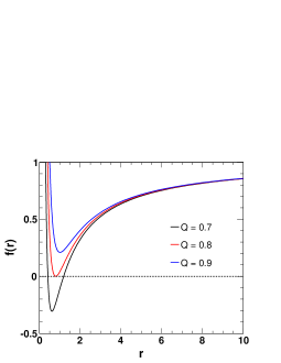
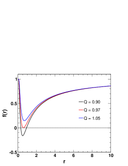
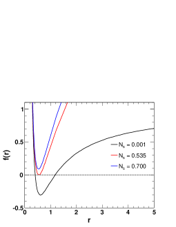
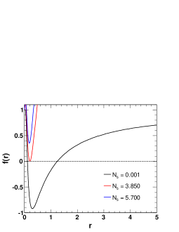
Figure 1: Variation of the metric function for the black holes defined by the metric (23) (on left) and metric (29) (on right) surrounded by quintessence field with a viable set of common parameters $\lambda=0.01$, $\kappa=1$ and $M=0.8$. The top panel is for different values of $Q$ with $N_{s}=0.001$ and the bottom panel is for different values of $N_{s}$ with $Q=0.7$.

     

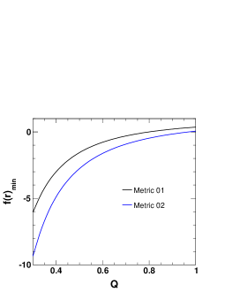
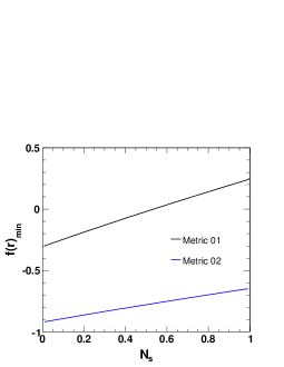
Figure 2: Variation of the minimum value of the metric function with respect to $Q$ and $N_{s}$ for the black holes surrounded by quintessence field with $\lambda=0.01$, $\kappa=1$ and $M=0.8$. Here the Metric 01 is defined by Eq. (23) and the Metric 02 is defined by Eq. (29). The left plot is for $N_{s}=0.001$ and the right plot is for $Q=0.7$.

For a black hole solution having mass function given by (28), it is possible to get the electric field from the field Eq. (3), if we define the energy momentum tensor $T_{\mu\nu}$ as

$$T_{\mu\nu}=L(F)g_{\mu\nu}-L_{F}F_{\mu\lambda}F^{\lambda}_{\nu}+{\mathcal{T}^{\mu}}_{\nu},$$ (30)

where $L(F)$ is an arbitrary function of $F=\dfrac{1}{4}F^{\mu\nu}F_{\mu\nu}$ (an Lorentz invariant) and $L_{F}=\dfrac{dL}{dF}$. Restricting the electric field by considering $F_{\mu\nu}=E(r)(\delta^{0}_{\mu}\delta^{1}_{\nu}-\delta^{1}_{\mu}\delta^{0}_{\nu})$, we can express the components of the field equation as

$${\Theta^{0}}_{0}={G^{0}}_{0}+\kappa\lambda R=\frac{1}{r^{2}}\big{[}f^{\prime}(r)r+f(r)-1\big{]}+\kappa\lambda R=\kappa\big{[}L(F)+E^{2}L_{F}-\rho(r)\big{]},$$ (31)

$${\Theta^{1}}_{1}={G^{1}}_{1}+\kappa\lambda R=\frac{1}{r^{2}}\big{[}f^{\prime}(r)r+f(r)-1\big{]}+\kappa\lambda R=\kappa\big{[}L(F)+E^{2}L_{F}-\rho(r)\big{]},$$

$${\Theta^{2}}_{2}={G^{2}}_{2}+\kappa\lambda R=\frac{1}{r^{2}}\big{[}rf^{\prime}(r)+\frac{1}{2}r^{2}f^{\prime\prime}(r)\big{]}+\kappa\lambda R=\kappa\big{[}L(F)+\dfrac{1}{2}\rho(r)(3\omega_{s}+1)\big{]},$$

$${\Theta^{3}}_{3}={G^{3}}_{3}+\kappa\lambda R=\frac{1}{r^{2}}\big{[}rf^{\prime}(r)+\frac{1}{2}r^{2}f^{\prime\prime}(r)\big{]}+\kappa\lambda R=\kappa\big{[}L(F)+\dfrac{1}{2}\rho(r)(3\omega_{s}+1)\big{]}.$$

The above mentioned restriction on the electric field confirms that the electric field is spherically symmetric, i.e. electric field does not depend on the $\theta$ and $\phi$ coordinates. This will be shown explicitly in the following part. One can also see that the restriction respects the asymmetric behaviour of $F_{\mu\nu}$. Further, the electromagnetic field equation $\nabla_{\mu}(F^{\mu\nu}L_{F})=0$ gives,

$$E(r)L_{F}=-\dfrac{Q}{4\pi r^{2}}.$$ (32)

Using the above result in Eq.s (31) and using the expression (20) we obtain,

$$E(r)=\frac{\pi Qe^{-\frac{Q^{2}}{2Mr}}\left(8Mr-Q^{2}\right)}{\kappa Mr^{3}}.$$ (33)

It is seen that the electric field is regular everywhere and asymptotically it results,

$$E(r)\approx\dfrac{Q}{r^{2}}.$$ (34)

This agrees with the result (11). We have calculated the Ricci scalar for the ansatz (29) as given by

$$R=\frac{Q^{4}e^{-\frac{Q^{2}}{2Mr}}}{2Mr^{5}}+\frac{3N_{s}(3\omega_{s}-1)\left[\kappa\lambda(\omega_{s}+1)-\omega_{s}\right]r^{-\frac{3(\omega_{s}+1)(4\kappa\lambda-1)}{3\kappa\lambda(\omega_{s}+1)-1}}}{\left[1-3\kappa\lambda(\omega_{s}+1)\right]^{2}},$$ (35)

the Ricci squared is

$$R_{\mu\nu}R^{\mu\nu}=\frac{e^{-\frac{Q^{2}}{Mr}}\left[4AMQ^{4}r^{2}+B+16M^{2}N_{s}\left(P^{2}-P-2\right)Q^{2}r^{P+4}e^{\frac{Q^{2}}{2Mr}}-8MQ^{6}r+Q^{8}\right]}{8M^{2}r^{10}},$$ (36)

where $A=8M-N_{s}P(P+1)r^{P+1}e^{\frac{Q^{2}}{2Mr}}$, $B=4M^{2}N_{s}^{2}(P+1)^{2}\left(P^{2}+4\right)r^{2P+6}e^{\frac{Q^{2}}{Mr}}$ and $P=\frac{3\omega_{s}-1}{3\kappa\lambda(\omega_{s}+1)-1}-2,$ and finally the Kretschmann scalar is found to be,

$$R_{\alpha\beta\mu\nu}R^{\alpha\beta\mu\nu} =$$ (37)

$$\left[\frac{N_{s}\big{(}6\kappa\lambda(\omega_{s}+1)-3\omega_{s}-1\big{)}\big{(}9\kappa\lambda(\omega_{s}+1)-3\omega_{s}-2\big{)}r^{-\frac{3(\omega_{s}+1)(4\kappa\lambda-1)}{3\kappa\lambda(\omega_{s}+1)-1}}}{\left[1-3\kappa\lambda(\omega_{s}+1)\right]^{2}}\right.$$

$$\left.-\frac{e^{-\frac{Q^{2}}{2Mr}}\left(8M^{2}r^{2}-8MQ^{2}r+Q^{4}\right)}{2Mr^{5}}\right]^{2}+\frac{4\left[N_{s}r^{\frac{3\omega_{s}-1}{3\kappa\lambda(\omega_{s}+1)-1}-2}-\frac{2Me^{-\frac{Q^{2}}{2Mr}}}{r}\right]^{2}}{r^{4}}$$

$$+\frac{4\left[\frac{e^{-\frac{Q^{2}}{2Mr}}\left(2Mr-Q^{2}\right)}{r^{3}}+\frac{N_{s}\big{(}-6\kappa\lambda(\omega_{s}+1)+3\omega_{s}+1\big{)}r^{\frac{-9\kappa\lambda(\omega_{s}+1)+3\omega_{s}+2}{3\kappa\lambda(\omega_{s}+1)-1}}}{3\kappa\lambda(\omega_{s}+1)-1}\right]^{2}}{r^{2}}.$$ (38)

From the expressions (35), (36) and (37) it is seen that for some selected values of $\omega_{s}$, $\lambda$ and $N_{s}$ it is possible to get a regular black hole from the metric (29). Thus we have obtained regular black hole solutions with non-linear electrodynamic sources in Rastall gravity. In the next part of the work, we’ll see the situations explicitly in which we can obtain regular black hole solutions for the ansatz and how the quasinormal modes of the corresponding black holes change.

IV Quasinormal Modes of Black holes in Rastall Gravity

In this section, we would like to study the quasinormal modes of two types black holes viz., one defined by the metric (23) and the other, a black hole with non-linear electrodynamic sources, defined by another metric (29). Here we consider 5 types of surrounding fields viz., dust field, radiation field, quintessence field, cosmological field and phantom field, and calculate the quasinormal modes for each case. At first, we perturb the black hole with some probe minimally coupled to a scalar field the having the equation of motion,

$$\dfrac{1}{\sqrt{-g}}\partial_{\alpha}(\sqrt{-g}g^{\alpha\beta}\partial_{\beta})\Phi^{m}_{l}=\mu^{2}\Phi^{m}_{l},$$ (39)

here $\mu^{2}$ is the mass square of the scalar field. It is possible and convenient to express the scalar field $\Phi$ in the form of spherical waves as

$$\Phi^{m}_{l}(t,r,\theta,\phi)=e^{-i\omega t}\dfrac{\psi(r)}{r}Y^{m}_{l}(\theta,\phi),$$ (40)

where $\psi(r)$ is the radial part, $Y^{m}_{l}(\theta,\phi)$ is the well known spherical harmonics and $\omega$ is the frequency of oscillations of time part of the wave. This $\omega$ will correspond to the quasinormal mode frequencies of black hole solutions as will be clear from the below. Using Eq. (40), we can transform Eq. (39) into a Schrödinger like equation, given by

$$\dfrac{d^{2}\psi}{dx^{2}}+\left[\omega^{2}-V_{l}(x)\right]\psi=0,$$ (41)

where $x$ is defined as

$$x=\int\dfrac{dr}{f(r)},$$ (42)

which is known as tortoise coordinate. In Eq. (41), the effective potential is

$$V_{l}(r)=f(r)\left\{\dfrac{f^{\prime}(r)}{r}+\dfrac{l(l+1)}{r^{2}}+\mu^{2}\right\}.$$ (43)

In this study, we’ll be interested in the massless scalar field only. Thus throughout this whole study, we’ll set $\mu=0$. For physical consistency, appropriate boundary conditions should be applied to Eq. (41) both at the horizon of the black hole and infinity. For asymptotically flat spacetimes, the quasinormal conditions are Ferrari ; Vishveshwara ,

$$\psi(x)\rightarrow\begin{cases}Ae^{+i\omega x}\;\;\;\text{if}\;\;x\rightarrow-\infty\\ Be^{-i\omega x}\;\;\;\text{if}\;\;x\rightarrow+\infty\end{cases},$$ (44)

where $A$ and $B$ are constants. The purely ingoing wave physically expresses that nothing can escape from the horizon of the black hole. On the other hand, the purely outgoing wave expresses that no radiation comes from the infinity. These two expressions precisely give the quasinormal requirement or condition which ensures the existence of infinite set of discrete complex numbers, known as quasinormal modes. For a normal Schwarzschild black hole, omitting electric charge, the quasinormal modes basically depend on the mass M only. This is in accordance with the no hair theorem Carter1971 ; Israel1967 and it is a significant outcome of GR. This theorem simply states that the black holes are simple objects and a few observable properties, such as mass, electric charge and angular momentum can completely describe them. In other words, the quasinormal modes of a charge-less black hole in GR can be simply characterized by mass $M$ and overtone $l$ of the black hole Bustillo ; Gurlebeck . But for the black holes defined by the metric (23) and (29), it is seen that, apart from mass $M$, the parameters $N_{s}$, $Q$ and $\lambda$ affect the quasinormal modes significantly. In this work we have used 5th order and 6th order WKB approximation Kono2003 to estimate the quasinormal frequencies.

The potential defined in Eq. (43) behaves differently for different surrounding fields of the black hole. To visualize this we have plotted the potential for different surrounding fields in Fig. 3 for both the black holes in Rastall gravity (defined by metrics (23) and (29)). It is seen that for the $r<2$ region, the behaviours of both the black holes are similar. The potential increases significantly with decrease in the value of $\omega_{s}$. For the phantom field the potential is having maximum value. For the quintessence field with $\omega_{s}=-2/3$, the potential decreases further and finally for the radiation field, the potential is having minimum values.

The variation of the potential with $l$ is shown in Fig.s 4 and 5 for phantom field and quintessence field respectively for the black hole with non-linear electrodynamic source in Rastall gravity. The Fig. 4 shows that with higher values of the structural constant $N_{s}$ in phantom field, the potential increases further after crossing the first bump (see the left plot). This anomalous behaviour can be diminished by decreasing the structural constant to a comparatively smaller value as shown in the right plot of this figure. Since all other fields behave similar to the quintessence field as clear from the Fig. 3, so the behaviour of the potential with $l$ would be similar to Fig. 5 for all other fields as in the case of the quintessence field.

To see the impacts of charge $Q$ and the structural parameter $N_{s}$ over the potential, we have further plotted the potential $V_{l}$ versus $r$ for different values of $Q$ and $N_{s}$ (see Fig. 6) for the quintessence field. The potential increases for increase in the values of $Q$ and $N_{s}$ and these results are in agreement with Fig. 2. These behaviours of $V_{l}$ will be similar for all other fields excluding the phantom field. However, for very small values of $N_{s}$ the phantom field potential will behave in a similar fashion.

     

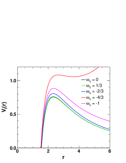
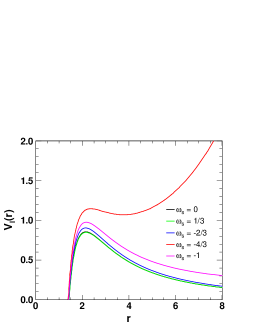
Figure 3: Behaviour of the potential $V_{l}(r)$ w. r. t. $r$ for black holes defined by the metric (23) (left plot) and metric (29) (right plot) with $l=3$, $Q=0.5$, $\lambda=0.01$, $\kappa=1$, $N_{s}=0.01$ and $M=0.8$ for different surrounding fields.

     

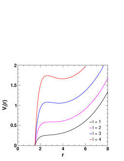
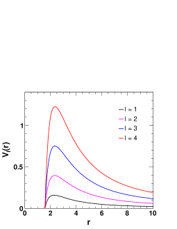
Figure 4: Variation of the potential $V_{l}(r)$ w. r. t. $r$ for black holes defined by the metric (29) surrounded by phantom field with $Q=0.2$, $\lambda=0.01$, $\kappa=1$, $M=0.8$ and $N_{s}=0.01$ (left plot) and $N_{s}=0.0001$ (right plot).

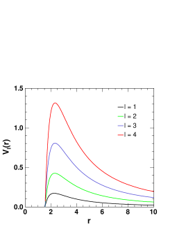
Figure 5: Variation of the potential $V_{l}(r)$ w. r. t. $r$ for black holes defined by the metric (29) surrounded by quintessence field with $Q=0.2$, $\lambda=0.01$, $\kappa=1$, $M=0.8$ and $N_{S}=0.01$.

     

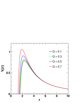
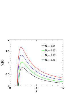
Figure 6: Behaviour of the potential $V_{l}(r)$ w. r. t. $r$ for black holes defined by the metric (29) surrounded by quintessence field with $l=3$, $\lambda=0.01$, $\kappa=1$ and $M=0.8$. For the plot on left $N_{s}=0.01$ and for the plot on right $Q=0.1$.

To see the dependency of the quasinormal modes on the surrounding fields, we have studied the corresponding black holes explicitly as follows.

IV.1 Surrounded by cosmological constant field

For the cosmological constant field, $\omega_{s}=-1$, the metrics (23) and (27) take the same form, which is

$$ds^{2}=-\left(1-\frac{2M}{r}+\frac{Q^{2}}{r^{2}}+r^{2}N_{s}\right)dt^{2}+\frac{dr^{2}}{1-\frac{2M}{r}+\frac{Q^{2}}{r^{2}}+r^{2}N_{s}}+r^{2}d\Omega^{2}.$$ (45)

This is identical to the metric obtained by Kiselev in GR Kiselev . It implies that the black hole metric behaves identically in both Rastall gravity and GR in cosmological constant background. Hence there will be no changes in the quasinormal modes in this case in comparison to the case in GR. Similarly, for this field the metric (29) with non-linear electrodynamic sources takes the following form,

$$ds^{2}=-\left(1-\frac{2m(r)}{r}+r^{2}N_{s}\right)dt^{2}+\frac{dr^{2}}{1-\frac{2m(r)}{r}+r^{2}N_{s}}+r^{2}d\Omega^{2},$$ (46)

For this metric, the Ricci scalar given in Eq. (35) takes the form,

$$R=\frac{Q^{4}e^{-\frac{Q^{2}}{2Mr}}}{2Mr^{5}}-12N_{s},$$ (47)

which is regular everywhere. Similarly, the Ricci squared and Kretschmann scalar are also regular everywhere. Thus the metric (46) represents a regular black hole with non-linear electrodynamic source. In Table 1, we have listed a few quasinormal mode frequencies for some selected parameters. To have an idea of the error associated with the calculations, we have calculated the deviations of 6th order WKB approximation from 5th order WKB approximation for all the cases. This deviation term is denoted by $|\omega_{5}-\omega_{6}|$, where $\omega_{5}$ represents quasinormal modes obtained by using the 5th order WKB approximation and $\omega_{6}$ represents quasinormal modes calculated by using the 6th order WKB approximation method. We have also calculated a quantity defined by Konoplya2019 ,

$$\vartriangle_{k}=|\dfrac{\omega_{k+1}-\omega_{k-1}}{2}|,$$

where $k$ denotes the order of WKB approximation. This quantity gives a good measurement of the error order Konoplya2019 . In this study, we have used this expression to calculate the error $\vartriangle_{5}$ associated with the 5th order WKB approximation. It is seen from the table that the quasinormal mode frequencies depend on the metric as well as on the multipole number $l$. This observation is applicable to quasinormal frequencies for all the cases calculated in this work. Here, in case of 6th order WKB approximation, the real frequencies given by the metric (46) are slightly higher than that given by the metric (45) for $l<3$. But for the $l=3$ the situation is appeared in the reverse way. In case of the 5th order WKB approximation, the real frequencies given by the metric (46) are slightly lower than that given by the metric (45) for all cases. The anomaly in the real frequencies in case of the 6th order WKB approximation can be explained in the following way. One can see the Table 1, where we have calculated the corresponding deviations and errors associated with the calculation. It is clear from the table that the errors and deviations associated with $l=1$ and $l=2$ are comparatively high and in the case of $l=3$, they are lowest. Hence, the reverse pattern of real quasinormal frequencies calculated by the 6th order WKB approximation can be an implication of the errors. If it is true, then the real frequencies given by the metric (46) should be, in general, lower than that given by the metric (45). To understand the behaviour of variation of quasinormal modes with respect to the parameters $Q$ and $N_{s}$, we have plotted both the real and imaginary parts of frequencies $\omega_{R}$ and $\omega_{I}$ respectively with respect to these two parameters in Fig.s 7 and 8. The variation of quasinormal modes with respect to $N_{s}$ is almost similar for both the metrics defined by (23) and (29) for small values of charge $Q$. However, in case of the variation with respect to charge $Q$ of the black holes, we notice significant variations of quasinormal modes for larger values of $Q$. It is seen that the magnitudes of both real and imaginary quasinormal modes are smaller for the regular black hole with non-linear charge distribution. This confirms the conclusion made on the results obtained in Table 1 i.e., the real quasinormal modes of the non-linearly charged black hole are expected to be lower. The asymptotic behaviours are identical and it is due to the choice of the distribution function as mentioned earlier.

     

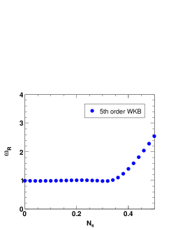
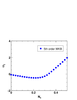
Figure 7: Fundamental quasinormal mode frequencies in terms of $N_{s}$ for the black holes defined by the metric (46) surrounded by cosmological constant field with $l=4$, $Q=0.2$ and $M=1$ obtained by using the 5th order WKB approximation method.

     

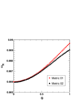
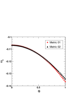
Figure 8: Fundamental quasinormal mode frequencies in terms of $Q$ for the black holes defined by the metric (45) (Metric 01) and (46) (Metric 02) surrounded by cosmological constant field with $l=4$, $N_{s}=0.01$ and $M=1$ obtained by using 5th order WKB approximation method.

	Metric (45)	Metric (46)
$l=1$ (6th order WKB)	$0.336678-0.10427i$	$0.338903-0.10357i$
$l=1$ (5th order WKB)	$0.339734-0.103332i$	$0.339723-0.10332i$
$|\omega_{5}-\omega_{6}|$	$0.00319671$	$0.000857263$
$\vartriangle_{5}$	$0.00178137$	$0.000904052$
$l=2$ (6th order WKB)	$0.553448-0.106688i$	$0.553569-0.106663i$
$l=2$ (5th order WKB)	$0.55353-0.106672i$	$0.553519-0.106673i$
$|\omega_{5}-\omega_{6}|$	$0.0000835464$	$0.0000509902$
$\vartriangle_{5}$	$0.0000425029$	$0.0000269258$
$l=3$ (6th order WKB)	$0.769435-0.107499i$	$0.76936-0.107509i$
$l=3$ (5th order WKB)	$0.769444-0.107498i$	$0.76943-0.107499i$
$|\omega_{5}-\omega_{6}|$	$9.05539\times 10^{-6}$	$0.0000707107$
$\vartriangle_{5}$	$5.31507\times 10^{-6}$	$0.000035203$

Table 1: Quasinormal modes of black holes for $n=0$, $M=1$, $\omega_{s}=-1$ (cosmological constant field), $N_{s}=0.01$ and $Q=0.2$.

In this case, the geometric parameter defined in Eq. (21) takes the following form Heydarzade2 ,

$$\mathcal{W}_{s}=-(1-4\kappa\lambda).$$ (48)

Hence, the weak energy condition (22) demands $N_{s}>0$ for $0\leq\kappa\lambda<\dfrac{1}{4}$ and $N_{s}<0$ for $\kappa\lambda>\dfrac{1}{4}$.

It is important to mention that both the black holes are independent of the Rastall parameter $\lambda$ and hence there will be no changes in the quasinormal modes for different values of this parameter.

IV.2 Surrounded by dust field

For the dust field, $\omega_{s}=0$ Kiselev ; Vikman and hence the metric (23) becomes,

$$ds^{2}=-\left(1-\frac{2M}{r}+\frac{Q^{2}}{r^{2}}+\frac{N_{s}}{r^{\frac{1-6\kappa\lambda}{1-3\kappa\lambda}}}\right)dt^{2}+\frac{dr^{2}}{1-\frac{2M}{r}+\frac{Q^{2}}{r^{2}}+\frac{N_{s}}{r^{\frac{1-6\kappa\lambda}{1-3\kappa\lambda}}}}+r^{2}d\Omega^{2}.$$ (49)

This metric has a different form in comparison to the similar case in GR Kiselev ; Heydarzade . Thus we expect variation in the quasinormal modes for this solution. Similarly for the metric (29), we have for dust field,

$$ds^{2}=-\left(1-\frac{m(r)}{r}+\frac{N_{s}}{r^{\frac{1-6\kappa\lambda}{1-3\kappa\lambda}}}\right)dt^{2}+\frac{dr^{2}}{1-\frac{2m(r)}{r}+\frac{N_{s}}{r^{\frac{1-6\kappa\lambda}{1-3\kappa\lambda}}}}+r^{2}d\Omega^{2}.$$ (50)

For the limit $\lambda\rightarrow 0$, the above metric can result black hole solutions similar to those found in Kiselev with a mass distribution function similar to Balart . One can easily recover the black hole solutions found in Balart in the limit $N_{s}\rightarrow 0$. Another interesting point mentioned for the metric (49) in Heydarzade2 is that, in the limit $\lambda\rightarrow 0$, the structural constant behaves more like a contribution to the mass of the black hole, where the modified mass term can be given as $(M-N_{s})$. Similarly, in this limit, the other black hole with non-linear electrodynamic source will also have a modified mass distribution function given by $(m(r)-N_{s})$. In this case, the black hole will be a regular black hole for any value of the parameter $N_{s}$. Thus it is seen that the structural parameter or constant $N_{s}$ can mimic the behaviour of mass of the black hole in the limit $\lambda\rightarrow 0$.

Here, the geometric parameter $\mathcal{W}_{s}$ is (Eq. (21))

$$\mathcal{W}_{s}=-\frac{\kappa\lambda\left(1-4\kappa\lambda\right)}{(1-3\kappa\lambda)^{2}}.$$ (51)

The weak energy condition for this type of black holes (for both) are given by, $0\leq\kappa\lambda<\frac{1}{4}$ demands $N_{s}>0$, and $\kappa\lambda<0~{}\cup~{}\kappa\lambda>\frac{1}{4}$, demands $N_{s}<0$ for the structural constant Heydarzade2 .

The quasinormal modes for both cases are shown in Table 2. The metrics (49) and (50) give the different values of quasinormal modes in comparison to the case of GR. Further, a similar observation can be made here in relation to $l$ as in the case of the cosmological constant field. The deviations of quasinormal modes obtained by using the 5th order and 6th order WKB approximations i.e., $|\omega_{5}-\omega_{6}|$ and error term associated with the 5th order WKB approximation $\vartriangle_{5}$ show that the errors are higher for smaller values of $l$ and for $l=3$, the errors are lowest. Hence, the quasinormal modes with higher $l$ value, more precisely higher $(l-n)$ values can have less errors in WKB approximation. Due to this reason, in the graphical analysis part, we have used $l=4$ and $n=0$. Again, the deviations of quasinormal modes obtained by using the 6th order WKB approximation of non-linearly charged black hole in Rastall gravity from the Reissner-Nordström black hole $\triangle_{NL-GR}$ are higher than that corresponding to linearly charged black hole in Rastall gravity from the Reissner-Nordström black hole $\triangle_{L-GR}$. However, in the case of 5th order WKB approximation both $\triangle_{NL-GR}$ and $\triangle_{L-GR}$ are of similar order. From the following part, it can be seen that with higher charge $(Q)$ values, these deviations may increase.

	Metric (49)	Metric (27)	Metric (50)	$\triangle_{NL-GR}$	$\triangle_{L-GR}$
$l=1$ (6th order WKB)	$0.296996-0.0983033i$	$0.296422-0.098453i$	$0.30379-0.0960863i$	$2.47764\%$	$0.189919\%$
$l=1$ (5th order WKB)	$0.296621-0.0984277i$	$0.296569-0.0984042i$	$0.296608-0.0984128i$	$0.0127811\%$	$0.0182622\%$
$|\omega_{5}-\omega_{6}|$	$0.000395095$	$0.000154888$	$0.00754942$
$\vartriangle_{5}$	$0.000259325$	$0.000185536$	$0.00377913$
$l=2$ (6th order WKB)	$0.489542-0.0974789i$	$0.48941-0.0974632i$	$0.494892-0.0964322i$	$1.11781\%$	$0.0266383\%$
$l=2$ (5th order WKB)	$0.48951-0.0974851i$	$0.489425-0.0974603i$	$0.4895-0.0974943i$	$0.0165012\%$	$0.0177431\%$
$|\omega_{5}-\omega_{6}|$	$0.0000325951$	$0.0000152778$	$0.00549561$
$\vartriangle_{5}$	$0.0000286051$	$0.000024683$	$0.00274767$
$l=3$ (6th order WKB)	$0.683541-0.0972213i$	$0.68341-0.0971983i$	$0.682585-0.0973599i$	$0.121787\%$	$0.0192679\%$
$l=3$ (5th order WKB)	$0.683532-0.0972226i$	$0.683413-0.0971979i$	$0.683516-0.0972274i$	$0.0155212\%$	$0.0176066\%$
$|\omega_{5}-\omega_{6}|$	$9.0934\times 10^{-6}$	$3.02655\times 10^{-6}$	$0.000940381$
$\vartriangle_{5}$	$7.43303\times 10^{-6}$	$5.87133\times 10^{-6}$	$0.000470279$

Table 2: Quasinormal modes of black holes for $n=0$, $M=1$, $\omega=0$ (dust field), $\kappa\lambda=0.01$, $N_{s}=0.01$ and $Q=0.2$.

To see the variations of quasinormal mode frequencies with respect to the structural constant $N_{s}$ we have plotted the quasinormal frequencies versus $N_{s}$ in Fig. 9, where the frequencies are calculated by using the 5th order WKB approximation method. Since the asymptotic behaviour of both the black holes are identical for smaller charges, we have shown the variations for the second black hole with non-linear electrodynamic source only. From Fig. 9 it is clear that the real quasinormal frequencies slightly increase for smaller region of $N_{s}$ (upto near $N_{s}=0.2$) giving rise to a small bump and beyond $N_{s}=0.5$ the frequencies decrease sharply. However, in case of the imaginary quasinormal frequencies, no such bump is observed and the frequencies fall off linearly with increasing values of $N_{s}$. It is important to mention that the magnitude of imaginary frequencies increase more rapidly in comparison to the real frequencies. To be precise, an increase in the parameter $N_{s}$ introduces more variations in the imaginary quasinormal frequencies.

Similar to the previous case, here also the quasinormal modes are dependent on the electrodynamic source of the black hole. The dependency of the frequencies on the charge $Q$ can be seen in Fig. 10. The variations are quite similar to that of the previous case.

     

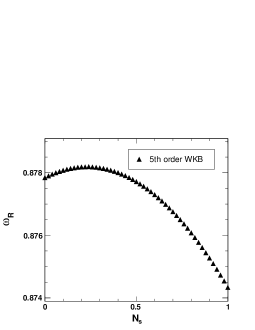
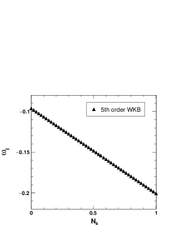
Figure 9: Fundamental quasinormal mode frequencies w. r. t. $N_{s}$ for the black holes defined by metric (50) surrounded by dust field with $l=4$, $\lambda=0.01$, $\kappa=1$, $Q=0.2$ and $M=1$ obtained by using the 5th order WKB approximation method.

     

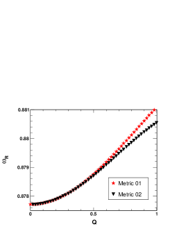
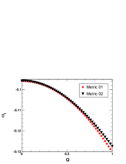
Figure 10: Fundamental quasinormal mode frequencies w. r. t. $Q$ for the black holes defined by metric (49) (Metric 01) and (50) (Metric 02) surrounded by dust field with $l=4$, $\lambda=0.01$, $\kappa=1$, $N_{s}=0.01$ and $M=1$ obtained by using the 5th order WKB approximation method.

     

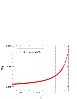
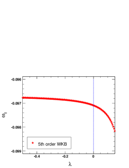
Figure 11: Fundamental quasinormal mode frequencies w. r. t. the Rastall parameter $\lambda$ for the black holes defined by the metric (50) surrounded by dust field with $l=4$, $Q=0.2$, $\kappa=1$, $N_{s}=0.01$ and $M=1$ obtained by using the 5th order WKB approximation method. The blue line shows the GR limit.

We have checked the dependency of quasinormal mode frequencies with respect to the Rastall parameter $\lambda$, which is shown in Fig. 11. It seen that the real quasinormal mode frequencies increase gradually with the increasing value of $\lambda$ upto the GR limit and after crossing this limit the frequencies increase rapidly with the increasing positive value of $\lambda$. On the other hand the magnitude of imaginary quasinormal mode frequencies increase with $\lambda$ following a similar pattern of the real frequencies before and after the GR limit of $\lambda$.

IV.3 Surrounded by phantom field

In case of phantom field $\omega_{s}=-\dfrac{4}{3}$ Vikman . Thus for this case the metric (23) becomes,

$$ds^{2}=-\left(1-\frac{2M}{r}+\frac{Q^{2}}{r^{2}}+\frac{N_{s}}{r^{\frac{-3+2\kappa\lambda}{1+\kappa\lambda}}}\right)dt^{2}+\frac{dr^{2}}{1-\frac{2M}{r}+\frac{Q^{2}}{r^{2}}+\frac{N_{s}}{r^{\frac{-3+2\kappa\lambda}{1+\kappa\lambda}}}}+r^{2}d\Omega^{2}.$$ (52)

Similarly metric (29) becomes,

$$ds^{2}=-\left(1-\frac{2m(r)}{r}+\frac{N_{s}}{r^{\frac{-3+2\kappa\lambda}{1+\kappa\lambda}}}\right)dt^{2}+\frac{dr^{2}}{1-\frac{2m(r)}{r}+\frac{N_{s}}{r^{\frac{-3+2\kappa\lambda}{1+\kappa\lambda}}}}+r^{2}d\Omega^{2}.$$ (53)

These solutions are different from the Kiselev black hole Kiselev . Here the Rastall parameter, charge and the structural constant play significant role in the variations of quasinormal frequencies. To see these variations, we have plotted Fig.s 12, 13 and 14. In Fig. 12 we see that an increase in the value of $N_{s}$ increases the real quasinormal frequencies. However, in case of the imaginary quasinormal frequencies, with increase in $N_{s}$, frequencies decrease more rapidly. Here $N_{s}$ acts as an damping factor increasing the damping rate. In this figure we have used the black hole defined by the metric (53). Again, for small values of charges, the quasinormal frequencies of black hole defined by the metric (52) coincides with that of the other black hole with non-linear electrodynamic sources (see Fig. 13). We found that the black hole with non-linear electrodynamic source i.e. the black hole defined by the metric (53), can result a regular or non-singular black hole if $\kappa\lambda<4$. The quasinormal frequencies of the black holes do not show any significant variation with respect to parameter $\lambda$. However, the frequencies show a discontinuous behaviour for a region with the value of $\lambda\leq-\,0.3$ (see Fig. 14). This is due to the fact that the phantom field potential becomes non feasible for the black hole solution for such values of $\lambda$. In this both cases, the geometric parameter $\mathcal{W}_{s}$ from Eq. (21) is obtained as

$$\mathcal{W}_{s}=-\dfrac{1}{3}\dfrac{(1-4\kappa\lambda)(4-\kappa\lambda)}{(1+\kappa\lambda)^{2}}.$$ (54)

From this expression, weak energy condition can be obtained. The weak energy condition allows $N_{s}>0$ for $0\leq\kappa\lambda<\frac{1}{4}~{}\cup~{}\kappa\lambda>4$ and $N_{s}<0$ for $\frac{1}{4}<\kappa\lambda<4$. The quasinormal modes for these black holes for $l=1$ to $3$ are shown in Table 3. In this case the metric (53) gives the smaller values of quasinormal modes than that given by the metric (52) for all three values of $l$ and all these frequencies are different in comparison to the case of GR. $|\omega_{5}-\omega_{6}|$ and $\vartriangle_{5}$ also show a similar pattern as in the previous cases. For the non-linearly charged black hole in Rastall gravity, both these terms give higher values. This is due to the non-linear charge distribution function as mentioned earlier. The deviation terms $\triangle_{NL-GR}$ and $\triangle_{L-GR}$ have equivalent order for $l=3$ in the case of both 5th order and 6th order WKB approximations. But, it is seen that for $l=1$ and $2$, in the case of 6th order WKB approximation, $\triangle_{NL-GR}$ is much higher than $\triangle_{L-GR}$. It can be due to the error associated with the approximation, because for the non-linear black hole with $l=1$ and $2$, both $|\omega_{5}-\omega_{6}|$ and $\vartriangle_{5}$ have higher values which can impact the results significantly.

	Metric (52)	Metric (27)	Metric (53)	$\triangle_{NL-GR}$	$\triangle_{L-GR}$
$l=1$ (6th order WKB)	$0.296112-0.0978824i$	$0.296164-0.0978612i$	$0.289416-0.10012i$	$2.28141\%$	$0.0180036\%$
$l=1$ (5th order WKB)	$0.296264-0.0978322i$	$0.296318-0.0978103i$	$0.296249-0.0978105i$	$0.0221124\%$	$0.0186743\%$
$|\omega_{5}-\omega_{6}|$	$0.000160075$	$0.000162194$	$0.00721274$
$\vartriangle_{5}$	$0.00018417$	$0.000183679$	$0.00361083$
$l=2$ (6th order WKB)	$0.488881-0.0970006i$	$0.488984-0.0969835i$	$0.487678-0.097239i$	$0.266948\%$	$0.0209444\%$
$l=2$ (5th order WKB)	$0.488896-0.0969976i$	$0.488999-0.0969805i$	$0.488884-0.0969991i$	$0.0233679\%$	$0.0209438\%$
$|\omega_{5}-\omega_{6}|$	$0.0000152971$	$0.0000152971$	$0.00122963$
$\vartriangle_{5}$	$0.0000245341$	$0.0000244845$	$0.000615288$
$l=3$ (6th order WKB)	$0.682603-0.0967835i$	$0.682748-0.0967698i$	$0.682546-0.0967902i$	$0.0294425\%$	$0.0211212\%$
$l=3$ (5th order WKB)	$0.682606-0.0967831i$	$0.682751-0.0967695i$	$0.68259-0.0967839i$	$0.0234409\%$	$0.0211197\%$
$|\omega_{5}-\omega_{6}|$	$3.02655\times 10^{-6}$	$3.01496\times 10^{-6}$	$0.0000444487$
$\vartriangle_{5}$	$5.82151\times 10^{-6}$	$5.82151\times 10^{-6}$	$0.0000230827$

Table 3: Quasinormal modes of black holes for $n=0$, $M=1$, $\omega=-\dfrac{4}{3}$ (phantom field), $\kappa\lambda=0.01$, $N_{s}=0.0001$ and $Q=0.2$.

     

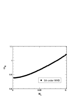
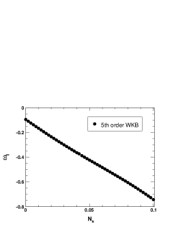
Figure 12: Behaviour of fundamental quasinormal mode frequencies w. r. t. $N_{s}$ for the black holes defined by the metric (53) surrounded by the phantom field with $l=4$, $\lambda=0.01$, $\kappa=1$, $Q=0.2$ and $M=1$ obtained using the 5th order WKB approximation method.

     

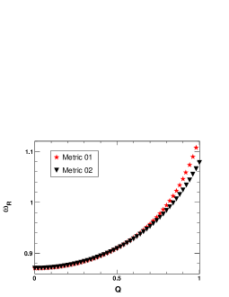
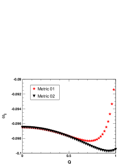
Figure 13: Behaviour of fundamental quasinormal mode frequencies w. r. t. $Q$ for the black holes defined by the metric (52) (Metric 01) and (53) (Metric 02) surrounded by phantom field with $l=4$, $\lambda=0.01$, $\kappa=1$, $N_{s}=0.0001$ and $M=1$ obtained by using the 5th order WKB approximation method.

     

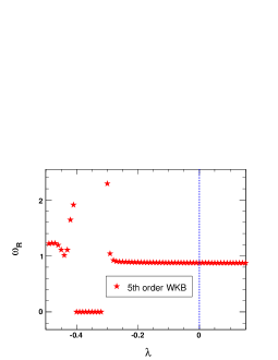
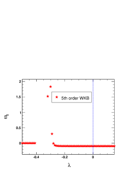
Figure 14: Behaviour of fundamental quasinormal mode frequencies w. r. t. the Rastall parameter $\lambda$ for the black holes defined by the metric (53) surrounded by the phantom field with $l=4$, $Q=0.2$, $\kappa=1$, $N_{s}=0.0001$ and $M=1$ obtained by using the 5th order WKB approximation method. The blue line shows GR limit.

IV.4 Surrounded by quintessence field

Using $\omega_{s}=-\dfrac{2}{3}$ for the quintessence field Kiselev , the metric (23) for this surrounding field can be written as

$$ds^{2}=-\left(1-\frac{2M}{r}+\frac{Q^{2}}{r^{2}}+\frac{N_{s}}{r^{\frac{-1-2\kappa\lambda}{1-\kappa\lambda}}}\right)dt^{2}+\frac{dr^{2}}{1-\frac{2M}{r}+\frac{Q^{2}}{r^{2}}+\frac{N_{s}}{r^{\frac{-1-2\kappa\lambda}{1-\kappa\lambda}}}}+r^{2}d\Omega^{2}.$$ (55)

Similarly, for this field the metric (29) becomes,

$$ds^{2}=-\left(1-\frac{2m(r)}{r}+\frac{N_{s}}{r^{\frac{-1-2\kappa\lambda}{1-\kappa\lambda}}}\right)dt^{2}+\frac{dr^{2}}{1-\frac{2m(r)}{r}+\frac{N_{s}}{r^{\frac{-1-2\kappa\lambda}{1-\kappa\lambda}}}}+r^{2}d\Omega^{2}.$$ (56)

The geometric parameter in these both cases takes the form,

$$\mathcal{W}_{s}=-\frac{\left(1-4\kappa\lambda\right)(2+\kappa\lambda)}{3(1-\kappa\lambda)^{2}}.$$ (57)

Using this parameter we can see that the black holes can respect the weak energy condition for $N_{s}>0$ with $0\leq\kappa\lambda<\frac{1}{4}$ and $N_{s}<0$ with $\kappa\lambda>\frac{1}{4}$ Heydarzade2 .

Here also both the black holes differ from Kiselev type black holes Kiselev ; Heydarzade2 . The second black hole with non-linear electrodynamic sources can result a regular or non-singular black hole if $\kappa\lambda<-2$. The variations of quasinormal modes with respect to charge for both the black holes are shown in Fig. 15. For the real quasinormal frequencies, with increase in charge $Q$, the frequencies increase non-linearly. However, similar to the other cases, the black hole with non-linear electrodynamic source or the regular black hole shows comparatively slower variation with respect to the singular black hole. In case of the imaginary quasinormal frequencies, there is a small dip in the variation pattern and near $1$ the frequencies increase again. In this region also the regular black hole has smaller quasinormal frequencies. These behaviours are very similar to the case of phantom field.

The behaviour of the quasinormal modes with the structural parameter $N_{s}$ for the regular black hole is shown in the Fig. 16. In both the cases increase in the parameter $N_{s}$ increases the damping rate. The increase in the magnitude of imaginary frequencies show that, with increase in $N_{s}$, the typical damping time decreases. The decrease in the frequencies are linear for both cases.

The Rastall parameter $\lambda$ introduces a significant signature on the quasinormal modes of the regular black hole (see Fig. 17). In case of the real quasinormal frequencies, an increase in $\lambda$ increases the frequencies non-linearly. Similarly, in case of the imaginary frequencies, the magnitude of the frequencies increase non-linearly but the variation is slower in comparison to the real frequencies. In both the plots, the blue line corresponds to the GR limit. The observational constraints on the Rastall parameter from Tang shows that in Rastall gravity, the magnitude of quasinormal modes will increase in comparison to GR. Quasinormal modes for $l=1$ to $3$ are shown in Table 4. For all three $l$ the quasinormal modes given by singular black hole are found to be larger than that for the case of GR. The deviations $|\omega_{5}-\omega_{6}|$ and error term $\vartriangle_{5}$ are comparatively smaller for the linearly charged black hole in Rastall gravity and GR. However, for the non-linearly charged black hole in Rastall gravity, they are higher as expected. It is due to the non-linear charge distribution function present in the non-linearly charged black hole. In general, the deviation of quasinormal modes of non-linearly charged black hole from the Reissner-Nordström black hole i.e., $\triangle_{NL-GR}$ is higher than that of linearly charged black hole in Rastall gravity from the Reissner-Nordström black hole $(\triangle_{L-GR})$. It is again due to the effect of the non-linear charge distribution function. The Fig. 15 suggests that $\triangle_{NL-GR}$ increases with increase in the value of charge $Q$ of the non-linearly charged black hole.

	Metric (55)	Metric (27)	Metric (56)	$\triangle_{NL-GR}$	$\triangle_{L-GR}$
$l=1$ (6th order WKB)	$0.295123-0.0979993i$	$0.295069-0.0980137i$	$0.274429-0.105352i$	$7.04541\%$	$0.0179746\%$
$l=1$ (5th order WKB)	$0.295221-0.0979667i$	$0.295216-0.097965i$	$0.295204-0.0979378i$	$0.00955789\%$	$0.00169785\%$
$|\omega_{5}-\omega_{6}|$	$0.00010328$	$0.000154857$	$0.0220584$
$\vartriangle_{5}$	$0.000175935$	$0.00018489$	$0.0110335$
$l=2$ (6th order WKB)	$0.487181-0.097029i$	$0.487159-0.0970304i$	$0.485045-0.0974635i$	$0.434425\%$	$0.00443794\%$
$l=2$ (5th order WKB)	$0.487181-0.0970289i$	$0.487173-0.0970274i$	$0.487171-0.097038i$	$0.00217156\%$	$0.00163856\%$
$|\omega_{5}-\omega_{6}|$	$1.0\times 10^{-7}$	$0.0000143178$	$0.00216816$
$\vartriangle_{5}$	$0.000023387$	$0.0000245775$	$0.00108475$
$l=3$ (6th order WKB)	$0.680272-0.0967685i$	$0.680259-0.0967672i$	$0.680935-0.0966769i$	$0.0992574\%$	$0.00190143\%$
$l=3$ (5th order WKB)	$0.680272-0.0967685i$	$0.680261-0.0967668i$	$0.680257-0.0967733i$	$0.00111077\%$	$0.00161992\%$
$|\omega_{5}-\omega_{6}|$	$0.$	$2.03961\times 10^{-6}$	$0.000684819$
$\vartriangle_{5}$	$5.73781\times 10^{-6}$	$5.82151\times 10^{-6}$	$0.000342457$

Table 4: Quasinormal modes of black holes for $n=0$, $M=1$, $\omega=-\dfrac{2}{3}$ (quintessence field), $\kappa\lambda=0.01$, $N_{s}=0.0001$ and $Q=0.2$.

     

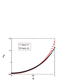
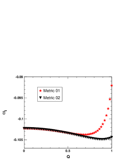
Figure 15: Fundamental quasinormal mode frequencies w. r. t. $Q$ for the black holes defined by the metric (55) (Metric 01) and (56) (Metric 02) surrounded by the quintessence field with $l=4$, $\lambda=0.01$, $\kappa=1$, $N_{s}=0.01$ and $M=1$ obtained by using the 5th order WKB approximation method.

     

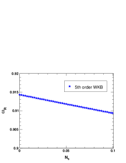
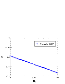
Figure 16: Fundamental quasinormal mode frequencies w. r. t. $N_{s}$ for the black holes defined by the metric (56) surrounded by the quintessence field with $l=4$, $\lambda=0.01$, $\kappa=1$, $Q=0.2$ and $M=1$ obtained by using the 5th order WKB approximation method.

     

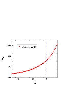
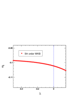
Figure 17: Fundamental quasinormal mode frequencies w. r. t. $\lambda$ for the black holes defined by the metric (56) surrounded by the quintessence field with $l=4$, $Q=0.2$, $\kappa=1$, $N_{s}=0.01$ and $M=1$ obtained by using the 5th order WKB approximation method. The blue line shows GR limit.

     

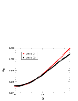
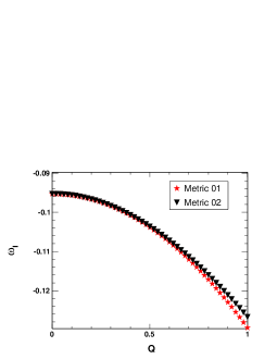
Figure 18: Fundamental quasinormal mode frequencies w. r. t. $Q$ for the black holes defined by the metric (58) (Metric 01) and (59) (Metric 02) surrounded by the radiation field with $l=4$, $N_{s}=0.01$ and $M=1$ obtained by using 5th order WKB approximation method.

     

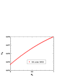
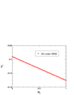
Figure 19: Fundamental quasinormal mode frequencies w. r. t. $N_{s}$ for the black holes defined by the metric (59) surrounded by the radiation field with $l=4$, $Q=0.2$ and $M=1$ obtained by using the 5th order WKB approximation method.

     

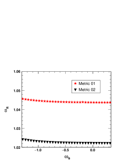
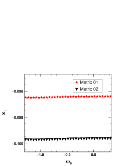
Figure 20: Variation of fundamental quasinormal mode frequencies w. r. t. $\omega_{s}$ for the black holes defined by the metric (23) (Metric 01) and (29) (Metric 02) with $l=4$, $\lambda=0.01$, $Q=0.9$, $\kappa=1$, $N_{s}=0.0001$ and $M=1$ obtained by using the 5th order WKB approximation method.

IV.5 Surrounded by radiation field

We can use the relativistic matter state parameter $\omega_{s}=\dfrac{1}{3}$ in order to denote any electrically charged black hole surrounded by static spherically symmetric electric field Kiselev . Hence, for the radiation field the metric (23) becomes,

$$ds^{2}=-\left(1-\frac{2M}{r}+\frac{Q^{2}}{r^{2}}+\frac{N_{s}}{r^{2}}\right)dt^{2}+\frac{dr^{2}}{1-\frac{2M}{r}+\frac{Q^{2}}{r^{2}}+\frac{N_{s}}{r^{2}}}+r^{2}d\Omega^{2}.$$ (58)

This metric is same as the metric in the GR limit for this field (see the metric (27)). That is the radiation field surrounded singular black holes are same for GR and Rastall gravity. For the radiation field the Metric (29) becomes,

$$ds^{2}=-\left(1-\frac{2m(r)}{r}+\frac{N_{s}}{r^{2}}\right)dt^{2}+\frac{dr^{2}}{1-\frac{2m(r)}{r}+\frac{N_{s}}{r^{2}}}+r^{2}d\Omega^{2}.$$ (59)

From the above metric it is clear that the black hole with non-linear electrodynamic source can not result a regular black hole unless the structural parameter $N_{s}=0$. In other words, with non-vanishing structural parameter both the metrics results singular black holes. The geometric parameter for both the black holes is

$$\mathcal{W}_{s}=\frac{1}{3}.$$ (60)

Thus to respect the weak energy condition, one needs $N_{s}\leq 0$. The metric (58) clearly shows that the charge $Q$ and the parameter $N_{s}$ terms can be combined to have $\frac{Q^{2}+N_{s}}{r^{2}}$ i.e., $N_{s}$ contributes to the square of charge in the metric in the case of the radiation field. This implies that for the radiation field, $N_{s}$ can behave as the square of some arbitrary charge. But $N_{s}<0$ predicts an imaginary charge behaviour and that may not be a physical situation to consider. However, in Fig.s 18, 19 and 20, we have considered positive $N_{s}$ values to compare the results with the previous cases although such values of $N_{s}$ do not respect the weak energy condition. We suggest that the case $N_{s}=0$ will be the most feasible case for a physically acceptable black hole as it is the only value that has no issues with the weak energy condition and imaginary charge problem.

In this surrounding field case, the black hole solutions are independent of the Rastall parameter $\lambda$ i.e., the black holes represented by the metrics in the radiation field are in fact the GR black holes. The variations of quasinormal modes with respect to charge $Q$ and the structural parameter $N_{s}$ are shown in Fig. 18 and 19 respectively. The variations of the frequencies with respect to the charge $Q$ is almost similar to the previous cases. However, in case of the imaginary frequencies, the bump is not present near $Q=1$. The magnitude of quasinormal frequencies increase with increase in the value of $N_{s}$. The quasinormal modes for $l=1$ to $3$ are shown in Table 5. Here the quasinormal modes calculated using 6th order WKB approximation show the similarpattern as that in case of cosmological constant field.

	Metric (58)	Metric (59)
$l=1$ (6th order WKB)	$0.294925-0.0979592i$	$0.320666-0.0901262i$
$l=1$ (5th order WKB)	$0.295071-0.0979107i$	$0.295074-0.0979431i$
$|\omega_{5}-\omega_{6}|$	$0.000153845$	$0.0267592$
$\vartriangle_{5}$	$0.000184587$	$0.0133854$
$l=2$ (6th order WKB)	$0.486938-0.0969744i$	$0.491358-0.0960924i$
$l=2$ (5th order WKB)	$0.486953-0.0969714i$	$0.486939-0.0969644i$
$|\omega_{5}-\omega_{6}|$	$0.0000152971$	$0.00450421$
$\vartriangle_{5}$	$0.0000245277$	$0.00225202$
$l=3$(6th order WKB)	$0.679958-0.0967107i$	$0.679922-0.0967148i$
$l=3$ (5th order WKB)	$0.67996-0.0967104i$	$0.679944-0.0967117i$
$|\omega_{5}-\omega_{6}|$	$2.02237\times 10^{-6}$	$0.0000222173$
$\vartriangle_{5}$	$5.82151\times 10^{-6}$	$0.0000126752$

Table 5: Quasinormal modes of black holes for $n=0$, $M=1$, $\omega=\dfrac{1}{3}$ (radiation field), $N_{s}=0.0001$ and $Q=0.2$.

In the previous parts, the Tables 1, 2, 3, 4 and 5 show the quasinormal modes for $l=1,2$ and $3$ obtained by using both 5th order and 6th order WKB approximation method with errors. We observe some anomalies and reverse patterns in some tables corresponding to different surrounding fields. Moreover, from the variations of quasinormal modes w.r.t. charge $Q$, one can easily see that for the higher multipole $(l=4)$ values and towards higher values of charge $Q$, the non-linearly charged black hole always has smaller real frequencies. However, this pattern is also slightly affected by the surrounding field. But the reverse pattern observed in some cases can be due to the error in WKB approximation method. It is because the WKB approximation does not allow to calculate quasinormal modes corresponding to $n\geq l$ with the satisfactory accuracy Konoplya2019 and again for smaller $l$ values the error of the approximation method is likely to be high. Consequently, in all the cases, it is observed that the errors and deviations corresponding to $l=1$ and $2$ are higher than $l=3$. Moreover, higher orders of WKB approximations may not always result in less error Konoplya2019 . This can be a reason for higher fluctuations or anomalous patterns of quasinormal modes calculated using 6th order WKB approximation. Apart from these, in general, the deviations and errors are higher for the non-linear black hole. This can be due to the non-linear charge distribution function. Thus, as mentioned earlier, these reverse patterns for smaller $l$ values in some tables corresponding to different surrounding fields are most likely due to the errors associated with the approximation method.

Another observation obtained from all the cases is that the imaginary part of the quasinormal modes are more affected by the parameter $N_{s}$. From Eq. (20) along with the condition (22), one can see that the increase in the parameter $N_{s}$ increases the energy density and it eventually increases the damping. As a reason of which we can see a direct dependence of the imaginary quasinormal modes with the structural parameter $N_{s}$. However, for the nature of a field both $\rho_{s}(r)$ and $f(r)$ get affected and the quasinormal modes also vary accordingly.

Finally, to have a comparative picture, we have studied the variation of the quasinormal frequencies for the linearly charged black hole and the black hole with non-linear electrodynamic source in Rastall gravity with respect to the surrounding field in Fig. 20. The magnitude of both the frequencies decrease slowly with increase in the value of $\omega_{s}$ from phantom field to radiation field. Thus increasing the value of $\omega_{s}$ introduces a damping effect on the quasinormal frequencies. The effect of damping is small for the phantom field and maximum for the radiation field.

We have also considered the constrained values of the Rastall parameter $\lambda$ from Ref. Tang and calculated the fundamental quasinormal frequencies for $l=2$ for the black holes defined by the metrics (23) (charged black holes in Rastall gravity surrounded by a field), (27) (Reissner-Nordström black hole) and (29) (black hole in Rastall gravity surrounded by a field with non-linear electrodynamic sources) in Table 6. This table will help to check the viability of Rastall gravity from the future observational data of quasinormal modes of black holes. In this context it needs to mention that in the Ref. Tang , from the constraining of the Rastall parameter, authors found that Rastall gravity is equivalent to GR. In contrast, we would like to point out that the quasinormal modes of black holes for the same set of constraint values of the Rastall parameter are different from the quasinormal modes in GR. This is clear from the fact that different $\kappa\lambda$ constraint values give different quasinormal modes as seen from Table 6. It implies that Rastall gravity, as mentioned earlier, is not completely equivalent to GR although some results may show similar behaviour.

V Conclusion

At weak field regime, Rastall gravity is identical to GR. Hence, it shares the same numbers of polarization modes of GWs with that of GR. But in the strong field regime, the theory deviates significantly from the GR. We have obtained charged black hole solutions surrounded by different fields in Rastall gravity. To obtain a regular black hole solution, we have further modified the metric by introducing a non-linear distribution function. However, we have seen that, for non-zero structural parameter $N_{s}$, the solutions can give regular black holes only for some selected surrounding fields. Although, the quasinormal modes of black hole with non-linear electrodynamic source mimic with that from the other one in terms of linear charge distribution in asymptotic regime, we have seen a significant difference between these two black holes for the large values of charge $Q$. Such a deviation can be clearly observed in Fig. 20 where $Q=0.9$ is used. In all five cases of the surrounding fields, the real quasinormal frequencies increase with respect to charge of the black hole. However, for the black hole with non-linear charge distribution, the real quasinormal frequencies increase slowly. This work has shown that regular black holes can be obtained by introducing a non-linear electrodynamic source in the black hole metric of Rastall gravity for some selected surrounding fields with non-zero structural parameter $N_{s}$.

We have also shown the dependency of the quasinormal modes with respect to the Rastall parameter $\lambda$. Since, Rastall gravity shows deviation from GR only in presence of matter or non-zero curvature, a choice of surrounding field can be expected to have significant influences over the black hole metric in this theory. For cosmological constant field $(\omega_{s}=-1)$ and radiation field $(\omega_{s}=1/3)$, the black hole metrics are independent of the Rastall parameter. Thus, the quasinormal modes for the black holes surrounded by these fields are independent of the Rastall parameter. The prime changes in the quasinormal modes are reflected by the structural parameter $N_{s}$ and the charge $Q$ of the black holes only. For the other three fields, the quasinormal modes depend highly on the Rastall parameter. However, the choice of field imposes changes differently in the quasinormal modes as seen from this study. It is seen that for dust field and quintessence field, the magnitudes of real and imaginary quasinormal modes increase with increase in the Rastall parameter and the variation in the quasinormal modes is more in the case of dust field than that of quintessence and phantom fields.

Finally, in this work we have mainly considered two types of charged black holes in Rastall gravity defined by (23) and (29). Similar studies are done for uncharged black holes in Rastall gravity in Ref.s Graca ; Liang . In another similar work the authors considered a black hole in Rastall gravity surrounded by a cloud of strings Cai . In this study, they observed decrease of the quasinormal frequency with increase in the Rastall parameter. But in our case, the results are distinctly opposite for dust field and quintessence field. Scalar quasinormal modes of non-linear charged black holes in Rastall gravity are studied recently in Hu , in which they have showed a similar variation of quasinormal modes with respect to charge. However, in our work, we have considered a non-linear distribution function to modify the metric of a charged black hole surrounded by different fields in Rastall gravity. The quasinormal modes of such a black hole in Rastall gravity have not been studied till now to the best of our knowledge. So we think that this study will contribute towards our knowledge and understanding of black holes in Rastall gravity. Apart from this, the present study may contribute to the ongoing studies in the GW astronomy. After detection of the GW events, the possibility of detection of quasinormal modes has increased. In the GW events, the ringdown phase has a very weak signal-to-noise ratio which makes it difficult to extract significant results from it. In a recent study, a method has been introduced to detect the weak quasinormal modes from such GW events once design sensitivity of ground based detectors is achieved Costa ; Martynov . In another study, it is shown that second generation GWs detectors such as Advanced LIGO (aLIGO) Aasi , Advanced Virgo (AdV) Acernese and KAGRA Aso can play a very promising role in the detection of quasinormal modes Nakamura . In the near future, with sufficient experimental results on quasinormal modes, such studies will help to check the viability of Rastall gravity and to discover more about the black hole spacetime. This work can be further extended by generalizing the Rastall gravity with the various aspects of spacetime geometry. For example, the modified covariant conservation condition $\nabla_{\nu}T^{\mu\nu}=\lambda\nabla^{\mu}R$ can be further extended by modifying the geometry part. This modification can be of two types: one in which usual conservation of the energy-momentum tensor can be recovered at weak field limit and the other in which conservation of the energy-momentum tensor violates in both the strong and weak field limits. It will be interesting to see the impacts of such modifications on the quasinormal modes of black holes.

Galaxy	$\kappa\lambda$	$\chi^{2}/dof$	Non-linearly charged Rastall black hole	Reissner-Nordström black hole	Linearly charged Rastall black hole
(1)	(2)	(3)	(4)	(5)	(6)
F563-1	0.054	0.879	0.491994 - i0.096021  0.487031 - i0.096999	0.483776 - i0.096784   0.483753 - i0.096789	0.487037 - i0.096998   0.487042 - i0.096996
F568-3	0.154	0.866	0.483888 - i0.097674   0.487135 - i0.097023	0.483822 - i0.096821  0.483858 - i0.096814	0.487132 - i0.097025   0.487147 - i0.097022
F583-1	0.15	0.836	0.486820 - i0.097075  0.487127 - i0.097014	0.483838 - i0.096815   0.483851 - i0.096812	0.487151 - i0.097018   0.487139 - i0.097020
F571-8	0.143	0.882	0.487064 - i0.097024   0.487115 - i0.097014	0.483822 - i0.096813   0.483839 - i0.096810	0.487084 - i0.097026   0.487127 - i0.097017
F579-v1	0.048	0.13	0.489137 - i0.096563   0.487024 - i0.096982	0.483737 - i0.096790   0.483750 - i0.096788	0.486974 - i0.097009   0.487039 - i0.096996
F583-4	0.141	0.211	0.484901 - i0.097459   0.487113 - i0.097016	0.483837 - i0.096808  0.483836 - i0.096809	0.487063 - i0.097029   0.487124 - i0.097017
F730-v1	0.095	0.53	0.489195 - i0.096583   0.487059 - i0.097007	0.483788 - i0.096795   0.483782 - i0.096796	0.487035 - i0.097010   0.487070 - i0.097003
U5750	0.146	0.82	0.484517 - i0.097542   0.487121 - i0.097021	0.483836 - i0.096813   0.483844 - i0.096811	0.487144 - i0.097016   0.487132 - i0.097018
U11454	0.118	0.826	0.486740 - i0.097090  0.487084 - i0.097021	0.483776 - i0.096807   0.483805 - i0.096802	0.487074 - i0.097013   0.487093 - i0.097009
U11616	0.122	0.808	0.487093 - i0.097002   0.487085 - i0.097003	0.483810 - i0.096803  0.483809 - i0.096803	0.487044 - i0.097021   0.487098 - i0.097011
U11648	0.132	0.356	0.490119 - i0.096418  0.487100 - i0.097015	0.483798 - i0.096811  0.483822 - i0.096806	0.487086 - i0.097019   0.487111 - i0.097014
U11819	0.147	0.958	0.488775 - i0.096693   0.487123 - i0.097021	0.483852 - i0.096810   0.483846 - i0.096811	0.487111 - i0.097024   0.487134 - i0.097019
ESO0140040	0.083	0.757	0.489062 - i0.096604  0.487049 - i0.097003	0.483741 - i0.096800   0.483772 - i0.096793	0.487108 - i0.096992   0.487061 - i0.097002
ESO2060140	0.1	0.812	0.488801 - i0.096670   0.487065 - i0.097015	0.483772 - i0.096800   0.483786 - i0.096797	0.487016 - i0.097017   0.487075 - i0.097005
ESO3020120	0.135	0.397	0.484058 - i0.097626   0.487104 - i0.097016	0.483833 - i0.096806   0.483827 - i0.096807	0.487093 - i0.097019   0.487115 - i0.097015
ESO4250180	0.121	1.675	0.487036 - i0.097013   0.487084 - i0.097003	0.483772 - i0.096810   0.483808 - i0.096802	0.487136 - i0.097002   0.487097 - i0.097010

Table 6: Quasinormal modes of black holes for the fundamental quadrupolar mode $(n=0,l=2)$ with $N_{s}=0.0001$ and $Q=0.2$ with the Rastall parameter $\lambda$ obtained from best fitting results from the rotation curves of 16 LSB spiral galaxies Tang . Column (1), (2) and (3) are the name of galaxy, the fitting values of Rastall parameter $\kappa\lambda$ and the $\chi^{2}$ values, respectively. These values are taken from Tang and are calculated by using $\omega=-1/3$ i.e. for perfect fluid dark matter (PFDM) or quintessence matter. Column (4) shows the quasinormal modes for the black hole in Rastall gravity with non-linear electrodynamic source (Eq. 29), column (5) shows the quasinormal modes for Reissner-Nordström black hole (Eq. 27) and column (6) shows the quasinormal modes for charged singular black hole in Rastall gravity (Eq. 23). In columns (4), (5) and (6) values of first subcolumn are calculated using the 6th order WKB approximation method and second subcolumn are calculated using the 5th order WKB approximation method

References

- (1) C. M. Will, The Confrontation between General Relativity and Experiment, Living Rev. Relativ. 17, 4 (2014) [arXiv:gr-qc/0510072].
- (2) R. A. Hulse and J. H. Taylor, Discovery of a Pulsar in a Binary System, The Astrophysical Journal Letters 195, L51 (1975).
- (3) T. Damour and J. H. Taylor, Strong-Field Tests of Relativistic Gravity and Binary Pulsars, Phys. Rev. D 45, 1840 (1992).
- (4) K. S. Stelle, Renormalization of Higher-Derivative Quantum Gravity, Phys. Rev. D 16, 953 (1977).
- (5) A. G. Riess et al., Observational Evidence from Supernovae for an Accelerating Universe and a Cosmological Constant, The Astronomical Journal 116, 1009 (1998).
- (6) S. Perlmutter et al., Measurements of and from 42 High-Redshift Supernovae, ApJ 517, 565 (1999).
- (7) N. A. Bahcall, The Cosmic Triangle: Revealing the State of the Universe, Science 284, 1481 (1999).
- (8) P. Bull et al., Beyond CDM: Problems, Solutions, and the Road Ahead, Physics of the Dark Universe 12, 56 (2016).
- (9) D. Liang, Y. Gong, S. Hou and Y. Liu, Polarizations of Gravitational Waves in Gravity, Phys. Rev. D 95, 104034 (2017) [arXiv:1701.05998].
- (10) D. J. Gogoi and U. D. Goswami, A New f(R) Gravity Model and Properties of Gravitational Waves in It, Eur. Phys. J. C 80, 1101 (2020) [arXiv:2006.04011].
- (11) D. J. Gogoi and U. D. Goswami, Gravitational Waves in Gravity Power Law Model, Indian J. Phys. (2021) [arXiv:1901.11277].
- (12) P. Rastall, Generalization of the Einstein Theory, Phys. Rev. D 6, 3357 (1972).
- (13) R. Saleem and Shahnila, Cosmological Evolution via Interacting/Non-Interacting Holographic Dark Energy Model for Curved FLRW Space–Time in Rastall Gravity, Physics of the Dark Universe 32, 100808 (2021).
- (14) K. A. Bronnikov, V. A. G. Barcellos, L. P. de Carvalho, and J. C. Fabris, The Simplest Wormhole in Rastall and K-Essence Theories, Eur. Phys. J. C 81, 395 (2021).
- (15) S. Ghosh, S. Dey, A. Das, A. Chanda, and B. C. Paul, Study of Gravastars in Rastall Gravity, J. Cosmol. Astropart. Phys. 07, 004 (2021).
- (16) M. F. A. R. Sakti and F. P. Zen, CFT Duals on Rotating Charged Black Holes Surrounded by Quintessence, Physics of the Dark Universe 31, 100778 (2021).
- (17) S. K. Maurya and F. Tello-Ortiz, Decoupling Gravitational Sources by MGD Approach in Rastall Gravity, Physics of the Dark Universe 29, 100577 (2020).
- (18) M. Visser, Rastall Gravity Is Equivalent to Einstein Gravity, Physics Letters B 782, 83 (2018) [arXiv:1711.11500].
- (19) F. Darabi, H. Moradpour, I. Licata, Y. Heydarzade, and C. Corda, Einstein and Rastall Theories of Gravitation in Comparison, Eur. Phys. J. C 78, 25 (2018).
- (20) W. A. G. De Moraes and A. F. Santos, Lagrangian Formalism for Rastall Theory of Gravity and Gödel-Type Universe, Gen. Relativ. Gravit. 51, 167 (2019).
- (21) H. Shabani and A. Hadi Ziaie, A Connection between Rastall-Type and f(R, T) Gravities, EPL 129, 20004 (2020).
- (22) A. S. Al-Rawaf and M. O. Taha, Cosmology of General Relativity without Energy-Momentum Conservation, Gen. Relat. Gravit. 28, 935 (1996).
- (23) A. S. Al-Rawaf and M. O. Taha, A Resolution of the Cosmological Age Puzzle, Physics Letters B 366, 69 (1996).
- (24) J. C. Fabris, R. Kerner, and J. Tossa, Perturbative analysis of generalized Einstein theories, Int. J. Mod. Phys. D 09, 111 (2000).
- (25) A.-M. M. Abdel-Rahman and M. H. A. Hashim, Gravitational Lensing in A Model With Non-Interacting Matter and Vacuum Energies, Astrophys. Space Sci. 298, 519 (2005).
- (26) A.-M. M. Abdel-Rahman, Gravitational Lensing Effects in a Modified General Relativity Model, Astrophys. Space Sci. 278, 385 (2001).
- (27) H. Moradpour, N. Sadeghnezhad, and S. H. Hendi, Traversable Asymptotically Flat Wormholes in Rastall Gravity, Can. J. Phys. 95, 1257 (2017).
- (28) K. D. Kokkotas and B. G. Schmidt, Quasi-Normal Modes of Stars and Black Holes, Living Rev. Relativ. 2, 2 (1999).
- (29) C. V. Vishveshwara, Stability of the Schwarzschild Metric, Phys. Rev. D 1, 2870 (1970).
- (30) W. H. Press, Long Wave Trains of Gravitational Waves from a Vibrating Black Hole, ApJ 170, L105 (1971).
- (31) S. Chandrasekhar and S. Detweiler, The Quasi-Normal Modes of the Schwarzschild Black Hole, Proc. R. Soc. Lond. A 344, 441 (1975).
- (32) E. Berti et al.,Testing General Relativity with Present and Future Astrophysical Observations, Class. Quantum Grav. 32, 243001 (2015).
- (33) O. Dreyer et al., Black-Hole Spectroscopy: Testing General Relativity through Gravitational-Wave Observations, Class. Quantum Grav. 21, 787 (2004).
- (34) A. M. Oliveira, H. E. S. Velten, J. C. Fabris and L. Casarini, Neutron Stars in Rastall Gravity, Phys. Rev. D 92, 044020 (2015) [arXiv:1506.00567].
- (35) Y. Heydarzade, H. Moradpour, and F. Darabi, Black Hole Solutions in Rastall Theory, Can. J. Phys. 95, 1253 (2017) [arXiv:1610.03881].
- (36) Y. Heydarzade and F. Darabi, Black Hole Solutions Surrounded by Perfect Fluid in Rastall Theory, Physics Letters B 771, 365 (2017) [arXiv:1702.07766].
- (37) S. Chen, J. Jing, Quasinormal modes of a black hole surrounded by quintessence Class. Quantum Gravity 22, 4651 (2005) [arXiv:gr-qc/0511085].
- (38) Y. Zhang, Y.X. Gui, Quasinormal modes of gravitational perturbation around a Schwarzschild black hole surrounded by quintessence, Class. Quantum Gravity 23, 6141 (2006) [arXiv:gr-qc/0612009].
- (39) Y. Zhang, Y.X. Gui, F. Li, Quasinormal modes of a Schwarzschild black hole surrounded by free static spherically symmetric quintessence: electromagnetic perturbations, Gen. Relativ. Gravit. 39, 1003 (2007) [arXiv:gr-qc/0612010].
- (40) C. Ma, Y. Gui, W. Wang, F. Wang, Massive scalar field quasinormal modes of a Schwarzschild black hole surrounded by quintessence, Cent. Eur. J. Phys. 6, 194 (2008) [arXiv:gr-qc/0611146].
- (41) Y. Zhang, Y.X. Gui, F. Yu, Dirac quasinormal modes of a Schwarzschild black hole surrounded by free static spherically symmetric quintessence, Chin. Phys. Lett. 26, 030401 (2009) [arXiv:0710.5064].
- (42) J. P. M. Graça and I. P. Lobo, Scalar QNMs for Higher Dimensional Black Holes Surrounded by Quintessence in Rastall Gravity, Eur. Phys. J. C 78, 101 (2018) [arXiv:1711.08714].
- (43) J. Liang, Quasinormal Modes of the Schwarzschild Black Hole Surrounded by the Quintessence Field in Rastall Gravity, Commun. Theor. Phys. 70, 695 (2018).
- (44) Y. Hu, C.-Y. Shao, Y.-J. Tan, C.-G. Shao, K. Lin, and W.-L. Qian, Scalar Quasinormal Modes of Nonlinear Charged Black Holes in Rastall Gravity, EPL 128, 50006 (2020).
- (45) Z. Xu, X. Hou, X. Gong, and J. Wang, Kerr–Newman-AdS Black Hole Surrounded by Perfect Fluid Matter in Rastall Gravity, Eur. Phys. J. C 78, 513 (2018).
- (46) K. Lin and W.-L. Qian, Neutral Regular Black Hole Solution in Generalized Rastall Gravity, Chinese Phys. C 43, 083106 (2019) [arXiv:1812.10100].
- (47) L. Balart and E. C. Vagenas, Regular Black Holes with a Nonlinear Electrodynamics Source, Phys. Rev. D 90, 124045 (2014) [arXiv:1408.0306].
- (48) M. Tang, Z. Xu, and J. Wang, Observational Constraints on Rastall Gravity from Rotation Curves of Low Surface Brightness Galaxies, Chinese Phys. C 44, 085104 (2020) [arXiv:1903.01034].
- (49) V. V. Kiselev, Quintessence and Black Holes, Class. Quantum. Grav 20, 1187 (2003) [arXiv:gr-qc/0210040].
- (50) V. Ferrari and L. Gualtieri, Quasi-Normal Modes and Gravitational Wave Astronomy, Gen. Relativ. Gravit. 40, 945 (2008) [arXiv:0709.0657].
- (51) B. Carter, Axisymmetric Black Hole Has Only Two Degrees of Freedom, Phys. Rev. Lett. 26, 331 (1971).
- (52) W. Israel, Event Horizons in Static Vacuum Space-Times, Phys. Rev. 164, 1776 (1967).
- (53) N. Gürlebeck, No-Hair Theorem for Black Holes in Astrophysical Environments, Phys. Rev. Lett. 114, 151102 (2015).
- (54) J. C. Bustillo, P. D. Lasky, and E. Thrane, Black-Hole Spectroscopy, the No-Hair Theorem, and GW150914: Kerr versus Occam, Phys. Rev. D 103, 024041 (2021).
- (55) R. A. Konoplya, Quasinormal Behavior of the D -Dimensional Schwarzschild Black Hole and the Higher Order WKB Approach, Phys. Rev. D 68, 024018 (2003).
- (56) R. A. Konoplya, A. Zhidenko, and A. F. Zinhailo, Higher Order WKB Formula for Quasinormal Modes and Grey-Body Factors: Recipes for Quick and Accurate Calculations, Class. Quantum Grav. 36, 155002 (2019).
- (57) A. Vikman, Can Dark Energy Evolve to the Phantom?, Phys. Rev. D 71, 023515 (2005).
- (58) X.-C. Cai and Y.-G. Miao, Quasinormal Modes and Spectroscopy of a Schwarzschild Black Hole Surrounded by a Cloud of Strings in Rastall Gravity, Phys. Rev. D 101, 104023 (2020) [arXiv:1911.09832].
- (59) C. F. Da Silva Costa, S. Tiwari, S. Klimenko, and F. Salemi, Detection of (2,2) Quasinormal Mode from a Population of Black Holes with a Constructive Summation Method, Phys. Rev. D 98, 024052 (2018).
- (60) D. V. Martynov et al., Sensitivity of the Advanced LIGO Detectors at the Begining of Gravitational Wave Astronomy, Phys. Rev. D 93, 112004 (2016).
- (61) J. Aasi et al. (LIGO Scientific Collaboration), Advanced LIGO, Class. Quant. Grav. 32, 074001 (2015).
- (62) F. Acernese et al. (VIRGO Collaboration), Advanced Virgo: A second-generation interferometric gravitational wave detector, Class. Quant. Grav. 32, 024001 (2015).
- (63) Y. Aso, Y. Michimura, K. Somiya, M. Ando, O. Miyakawa, T. Sekiguchi, D. Tatsumi, and H. Yamamoto (KAGRA Collaboration), Interferometer design of the KAGRA gravitational wave detector, Phys. Rev. D 88, 043007 (2013).
- (64) T. Nakamura, H. Nakano, and T. Tanaka, Detecting Quasinormal Modes of Binary Black Hole Mergers with Second-Generation Gravitational-Wave Detectors, Phys. Rev. D 93, 044048 (2016).