Quantum Algorithms for Prediction Based on Ridge Regression

Abstract

We propose a quantum algorithm based on ridge regression model, which get the optimal fitting parameters $\vec{w}$ and a regularization hyperparameter $\alpha$ by analysing the training dataset. The algorithm consists of two subalgorithms. One is generating predictive value for a new input, the way is to apply the phase estimation algorithm to the initial state $\left|{X}\right\rangle$ and apply the controlled rotation to the eigenvalue register. The other is finding an optimal regularization hyperparameter $\alpha$, the way is to apply the phase estimation algorithm to the initial state $\left|{\vec{y}}\right\rangle$ and apply the controlled rotation to the eigenvalue register. The second subalgorithm can compute the whole training dataset in parallel that improve the efficiency. Compared with the classical ridge regression algorithm, our algorithm overcome multicollinearity and overfitting. Moreover, it have exponentially faster. What’s more, our algorithm can deal with the non-sparse matrices in comparison to some existing quantum algorithms and have slightly speedup than the existing quantum counterpart. At present, the quantum algorithm has a wide range of application and the proposed algorithm can be used as a subroutine of other quantum algorithms.

1 Introduction

With the amount of stored data globally increasing by about 20$\%$ every year[1], the pressure to find efficient approaches to machine learning is also growing[2]. At present, there are some interesting ideas that some researcherss exploit the potential of quantum computing to optimize algorithms of classical computing. In the past few decades, physicists have demonstrated the astonishing capacity of quantum system to process huge datasets[3]. Compared with the physical realization of traditional computer based on “0” and “1”, quantum computer can take advantage of the superposition of quantum states to realizes the goal of acceleration. However, the laws of quantum mechanics also limit our access to information stored in quantum systems[4,5], thus, it is a great challenge to find a better quantum algorithm over classical algorithm. Even so, there are a number of well-known improved quantum algorithms have been put forward. For example, Shor demonstrated that quantum algorithm of finding the prime factors of integer and so-called ‘discrete logarithm’ problem that could solved exponentially faster than any known classical algorithm in 1994[6]. Compared with the classical algorithms, the existing quantum algorithms have amazing speedup so that some researchers are considering whether these quantum algorithms can be applied to the filed of machine learning to solve the problems of low efficiency caused by the classical computers process big data.

As of now, a series of quantum algorithms about Linear Regression (LR) have been put forward. For example, Wiebe et al.[7] first provided a quantum linear regression algorithm that can efficiently solve data fitting over an exponentially large dataset by building upon an algorithm for solving systems of linear equations efficiently in 2012[8], but design matrice of their algorithm must be sparse. Hence, in 2016, Schuld et al.[9] came up with a quantum linear regression algorithm that can efficiently process the low-rank non-sparse design matrices. Although many such articles have been proposed, majority of these quantum linear regression algorithms are based on Ordinary Linear Regression (OLR) rather than Ridge Regression (RR). However, there are two intractable problems about multicollinearity and overfitting about LR. Thus, in 2017, Liu and Zhang[10] proposed an efficient quantum algorithm that can solve and combat questions about multicollinearity and overfitting. Nonetheless, Liu and Zhang don’t determine a good $\alpha$ for RR. So later, Yu et al.[11] presented an improved quantum ridge regression algorithm that proposed the parallel Hamiltonian simulation to obtain the optimal fitting parameters $\vec{w}$ and quantum K-fold cross validation to obtain an appropriate $\alpha$.

On the basis of previous papers, we further exploit how to extent RR algorithm can be faster by quantum computing than classical computing. Therefore, we design a more comprehensive quantum algorithm for RR. Inspired by quantum OLR of Schuld, we want to introduce a regularization hyperparameter $\alpha$ to the paper through analyzing data suffering from multicollinearity and overfitting. It is shown that our algorithm exponentially faster than classical counterpart when matrix is low-rank, but slightly worse on the error. To a certain extent, our algorithm have improved the existing quantum ridge regression algorithms[10, 11]. For example, we have a samll improvement compared with Yu’s algorithm, the dependence on conditional number $\kappa$ is slightly better.

The rest of this paper is organized as follows. In Section2, we review RR in terms of basic ideas and classical algorithmic procedures. In Section3, we present two important subalgorithms and their time complexity. In Section4, we analysis time complexity of two subalgorithm and whole algorithm. Conclusion is given in the Section5.

2 Preliminaries

In a simple linear regression model, a training set with M data points $\left({\vec{x}_{i},y_{i}}\right)_{i=1}^{M}$ is given. Here $\overrightarrow{{x_{i}}}={\left({{x_{i1}},{x_{i2}},\ldots,{x_{iN}}}\right)^{T}}\in{R^{N}}$ is a vector of N independent input variables, ${y_{i}}\in R$ is the scalar dependent output variables and target vector $\vec{y}={\left({{y_{1}},{y_{2}},\ldots,{y_{M}}}\right)^{T}}\in R^{M}$. The goal of LR algorithm is to obtain a vector of fitting parameters $\vec{w}$ from the training set, then utilize $\vec{w}$ to predict the result for a new input $\vec{x}^{\prime}$. Thus, we need to make the predictive values $f\left({{{\vec{x}}_{i}}}\right)$ as close as possible to real values ${y_{i}}$. Where $f\left({{{\vec{x}}_{i}}}\right)={\vec{x}_{i}}^{T}\vec{w}{\rm,}$.

A direct way to obtain optimal fitting parameters $\vec{w}$ is utilizing least squares method of minimizing the objective function

$$\mathop{\min}\limits_{w}{\left\|{X\vec{w}-\vec{y}}\right\|^{2}.}$$ (1)

where $X=\left({\vec{x}_{1},\vec{x}_{2},...,\vec{x}_{M}}\right)^{T}\in R^{M\times N}$. Thus, we can obtain fitting parameters $\vec{w}$, that is

$$\vec{w}={\left({X^{\dagger}X}\right)^{-1}}{X^{\dagger}}\vec{y},$$ (2)

Here, $X^{\dagger}$ is Hermitian conjugate or adjoint of the matrix X. The above regression is named as OLR.

However, in Ref.[12], Hoerl and Kennard pointed that OLR can encounter multicollinearity of independent variables of data points or overfitting from Eq. (1), so it is often far from satisfaction. To overcome the two problems, they put forward a new regression model – RR model, in which second normal form (2nd NF) of $\vec{w}$ is introduced. Thus, the objective function is changed to

$$\;\mathop{\min}\limits_{w}{\left\|{X\vec{w}-\vec{y}}\right\|^{2}}+\alpha{\left\|{\vec{w}}\right\|^{2}}.$$ (3)

Through simple calculation, the optimal fitting parameters $\vec{w}$ of the RR algorithm is

$$\vec{w}=\left({X^{\dagger}X+\alpha I}\right)^{-1}X^{\dagger}\vec{y},$$ (4)

Obviously, OLR is a particular case of RR that $\alpha=0$. For any matrix X, we take advantage of the singular value decomposition[13] to write $X=U\Sigma{V^{\dagger}}$. Here $\Sigma$ is a diagonal matrix containing the real singular values ${\lambda_{1}},{\lambda_{2}},\dots,{\lambda_{R}}>0$. Without loss of generality, we assume $\lambda_{r}\in\left[{\frac{1}{\kappa},1}\right]$ ($\kappa$ is the conditional number of matrix X), and the rth orthogonal column of ${U}\in{R^{M\times R}}\;({V}\;\in{R^{R\times N}})$ is left (right) eigenvector $\vec{u}_{r}\left(\vec{v}_{r}\right)$ corresponding to the singular value $\lambda_{r}$. Because the singular value decomposition can always be applied for any matrices, we let ${Z}\buildrel\Delta\over{=}\left({{X}^{\dagger}{X}+\alpha{I}}\right)^{-1}{X}^{\dagger}$, which can be represented as ${Z}={V}\Lambda{U}^{\dagger}$ by the singular value decomposition, where $\Lambda$ is a diagonal matrix containing the singular values ${\sigma_{1}}=\frac{{{\lambda_{1}}}}{{\lambda_{1}^{2}+\alpha}},{\sigma_{2}}=\frac{{{\lambda_{2}}}}{{\lambda_{2}^{2}+\alpha}},\dots,{\sigma_{R}}=\frac{{{\lambda_{R}}}}{{\lambda_{R}^{2}+\alpha}}$.

The following is the using of this mathematical background, X and Z have alternative expression formula $X=\sum\limits_{r}{\lambda_{r}}\vec{u}_{r}\vec{v}_{r}^{T}$ and $Z=\sum\limits_{r}{\sigma_{r}}\vec{v}_{r}\vec{u}_{r}^{T}$. So Eq. (4) can express as $\vec{w}=\sum\limits_{r=1}^{R}{\sigma_{r}\vec{v}_{r}\vec{u}_{r}^{T}\vec{y}}$. According to $f\left({\vec{x}_{i}}\right)=\vec{x}_{i}\vec{w}$, the corresponding output $y^{\prime}$ can be gained as follows for a new input $\vec{x}^{\prime}$,

$$y^{\prime}=\sum\nolimits_{r=1}^{R}{\sigma_{r}\vec{x}^{\prime}}\vec{v}_{r}\vec{u}_{r}^{T}\vec{y}.$$ (5)

The desired output is a single scalar value, but we need to get a vector for whole training set in algorithm 2. Thus, Eq. (5) must be performed many times. If so, the efficiency of algorithm is low in classical algorithm. Therefore, this work describe a quantum algorithm that can efficiently reproduce the whole result of a training dataset through parallelism of quantum computing.

3 Quantum algorithms for ridge regression

In this section, we design a quantum algorithm for RR. It contains two parts: a quantum algorithm for generating predictive value $y^{\prime}$ about a new input $\vec{x}^{\prime}$ and a quantum algorithm for finding an optimal regularization hyperparameter $\alpha$.

3.1 Algorithm 1: generating predictive values

3.1.1 The specific steps of algorithm 1

Given a training set of M data points $\left({\vec{x}_{i},y_{i}}\right)_{i=1}^{M}$, then we present a quantum algorithm to generate predictive values $y^{\prime}$ for a new input $\vec{x}^{\prime}$ that approximates to the real value $y$ within error $\varepsilon$. The algorithm 1 proceeds as following steps and the schematic is given in Fig. 1.

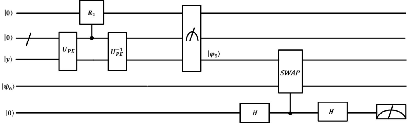
Figure 1: The whole quantum circuit for algorithm 1. Here the $U_{PE}$ and $U_{PE}^{-1}$ denote the phase estimation, the inverse phase estimation of the Step (2) and Step (3) respectively. The $R_{1}$ is controlled rotation of Step (3). SWAP is the original swap operation of Step (5).

Step (1) Preparing quantum state of $\vec{y}$, $\vec{x}^{\prime}$ and X respectively. The specific expressions are

$$\left|\vec{y}\right\rangle_{1}=\sum\limits_{i=0}^{M-1}{y_{i}\left|i\right\rangle_{1}}.$$ (6)

$$\left|\vec{x}^{\prime}\right\rangle_{2}=\sum\limits_{\gamma=0}^{N-1}{{x^{\prime}}_{\gamma}\left|\gamma\right\rangle_{2}},$$ (7)

$$\left|{X}\right\rangle_{34}=\sum\nolimits_{m=0}^{M-1}{\sum\nolimits_{n=0}^{N-1}{x_{mn}\left|m\right\rangle_{3}\left|n\right\rangle_{4}}},$$ (8)

According to reference[14], the procedure of preparing quantum state $\left|\vec{y}\right\rangle_{1}$ is as follows. Supposed, there is an oracle $O_{\vec{y}}$ that can access the elements of $\vec{y}$ in time $O(\log_{2}{\rm{M}})$ from quantum random access memory (QRAM) and acts as

$$O_{{y}}:\left|i\right\rangle_{1}\left|0\right\rangle_{a2}\to\left|i\right\rangle_{1}\left|{y_{i}}\right\rangle_{a2}.$$ (9)

Secondly, giving initial state $\left|0\right\rangle_{1}\left|0\right\rangle_{a2}$ and performing the quantum Fourier transform on $\left|0\right\rangle_{1}$, which gets $\sum\limits_{i=0}^{M-1}{\frac{{\left|i\right\rangle_{1}}}{{\sqrt{M}}}}$. The quantum Fourier transform on an orthonormal basis $\left|0\right\rangle,...,\left|{N-1}\right\rangle$ is defined to be a linear operator with the following action on the basis states,

$$\left|j\right\rangle\to\frac{1}{{\sqrt{N}}}\sum\limits_{k=0}^{N-1}{{e^{{{2\pi ijk}\mathord{\left/{\vphantom{{2\pi ijk}N}}\right.\kern-1.2pt}N}}}\left|k\right\rangle}.$$ (10)

Then, the oracle is applied to $\sum\limits_{i=0}^{M-1}{\frac{{\left|i\right\rangle_{1}\left|0\right\rangle_{a2}}}{{\sqrt{M}}}}$, which come into being $\sum\limits_{i=0}^{M-1}{\frac{{\left|i\right\rangle_{1}\left|{y_{i}}\right\rangle_{a2}}}{{\sqrt{M}}}}$. Thirdly, appending a qubit $\left|0\right\rangle_{a3}$ and performing controlled rotation for $\left|{y_{i}}\right\rangle_{a2}$ to generate the state

$$\sum\limits_{i=0}^{M-1}{\frac{{\left|i\right\rangle_{1}\left|{y_{i}}\right\rangle_{a2}}}{{\sqrt{M}}}}\left({\sqrt{1-\left({\frac{{y_{i}}}{{\left\|{\vec{y}}\right\|_{\max}}}}\right)^{2}}\left|0\right\rangle_{a3}+\frac{{y_{i}}}{{\left\|{\vec{y}}\right\|_{\max}}}\left|1\right\rangle_{a3}}\right).$$ (11)

In the next moment, uncomputing the oracle and generating the state

$$\sum\limits_{i=0}^{M-1}{\frac{{\left|i\right\rangle_{1}\left|0\right\rangle_{a2}}}{{\sqrt{M}}}\left({\sqrt{1-{{\left({\frac{{{y_{i}}}}{{\left\|{\vec{y}}\right\|}}}\right)}^{2}}}\left|0\right\rangle_{a3}+\frac{{{y_{i}}}}{{\left\|{\vec{y}}\right\|}}\left|1\right\rangle_{a3}}\right)}.$$ (12)

Finally, measuring the last register a3 in the basis $\left\{{\left|0\right\rangle,\left|1\right\rangle}\right\}$, which has probability $P_{y}=\frac{{\sum\limits_{i=0}^{M-1}{y_{i}^{2}}}}{{M\left\|{\vec{y}}\right\|_{\max}^{2}}}$. Generally, we assume that $\vec{y}$ is balanced ($\vec{x}^{\prime}$ and X is also same), so $P_{y}=\Omega\left(1\right)$. This implies that we need $O\left(1\right)$ measurements to obtain $\sum\limits_{i=0}^{M-1}{\frac{{y_{i}\left|i\right\rangle_{1}}}{{\sqrt{M}\left\|\vec{y}\right\|_{\max}}}}$. That is, we have a large probability to get the desired result. Moreover, the total time for generating the the results is $O(\log_{2}{\rm{M}})$. Thus, we can easily construct the quantum state $\left|\vec{y}\right\rangle_{1}$

$$\left|\vec{y}\right\rangle_{1}=\sum\limits_{i=0}^{M-1}{y_{i}\left|i\right\rangle_{1}}.$$ (13)

The same method is used to get the other two quantum states respectively.

$$\left|\vec{x}^{\prime}\right\rangle_{2}=\sum\limits_{\gamma=0}^{N-1}{{x^{\prime}}_{\gamma}\left|\gamma\right\rangle_{2}},$$ (14)

$$\left|{X}\right\rangle_{34}=\sum\nolimits_{m=0}^{M-1}{\sum\nolimits_{n=0}^{N-1}{x_{mn}\left|m\right\rangle_{3}\left|n\right\rangle_{4}}},$$ (15)

where $\sum\limits_{i}{{{\left|{{y_{i}}}\right|}^{2}}}=\sum\limits_{\gamma}{\left|{{x^{\prime}}_{\gamma}}\right|}^{2}=\sum\limits_{m,n}{{{\left|{{x_{mn}}}\right|}^{2}}}=1$. Then using the Gram-Schmidt decomposition[15], $\left|{X}\right\rangle_{34}$ can be re-expressed as

$$\left|{X}\right\rangle_{34}{\rm{=}}\sum\limits_{r=1}^{R}{\lambda_{r}}\left|{\vec{u}_{r}}\right\rangle_{3}\left|{\vec{v}_{r}}\right\rangle_{4}.$$ (16)

Here $\left|{{\vec{u}_{r}}}\right\rangle_{3}$ and $\left|{{\vec{v}_{r}}}\right\rangle_{4}$ are quantum states representing the orthogonal sets of left and right eigenvectors of $X$ respectively.

Step (2) In order to convert Eq. (16) to “quantum representation” of result (5), that is to say, quantum form of $y^{\prime}=\sum\nolimits_{r=1}^{R}{\sigma_{r}\vec{x}^{\prime}}\vec{v}_{r}\vec{u}_{r}^{T}\vec{y}$. We are first to extract the singular value $\lambda_{r}^{2}$ of $\emph{X}{\emph{X}^{\dagger}}$. Since X is generally not Hermitian, we extent it to a Hermitian matrix $\emph{X}{\emph{X}^{\dagger}}$. Then, we need to calculate the reduced density operator for the register $\left|{\vec{u}_{r}}\right\rangle_{3}$ of $\left|{X}\right\rangle_{34}$. So in that case, we can get a mixed state $\rho_{{X}{X}^{\dagger}}$.

$$\rho_{{X}{{X}^{\dagger}}}=tr_{4}\left\{{\left|{X}\right\rangle\left\langle{X}\right|}\right\}=\sum\nolimits_{r=1}^{R}{\lambda_{r}^{2}\left|{\vec{u}_{r}}\right\rangle}\left\langle{\vec{u}_{r}}\right|,$$ (17)

where $tr_{4}$ is known as the partical trace over the register $\left|{\vec{v}_{r}}\right\rangle_{4}$. Here, we take the trick of reference[16] to apply $e^{-i\rho_{{X}{{X}^{\dagger}}}q\Delta t}$ to $\left|{X}\right\rangle_{34}$ resulting in

$$\left|\varphi\right\rangle_{1}=\sum\nolimits_{q=1}^{Q}{\left|{q\Delta t}\right\rangle}\left\langle{q\Delta t}\right|e^{-i\rho_{{X}{{X}^{\dagger}}}q\Delta t}\left|{X}\right\rangle\left\langle{X}\right|e^{i\rho_{{X}{{X}^{\dagger}}}q\Delta t},$$ (18)

for some large Q. Then, by performing the quantum phase estimation algorithm on $\left|{X}\right\rangle_{34}$, we can get

$$\left|{\varphi_{2}}\right\rangle_{345}=\sum\nolimits_{r=1}^{R}{\lambda_{r}}\left|{\vec{u}_{r}}\right\rangle_{3}\left|{\vec{v}_{r}}\right\rangle_{4}\left|{\lambda_{r}^{2}}\right\rangle_{5}.$$ (19)

The phase estimation is performed in two stages. First, we run the quantum circuit shown in Fig. 2. The circuit begins by applying the quantum Fourier transform to the first register $\left|0\right\rangle$, followed by application of controlled unitary operation on the second register $\left|{X}\right\rangle_{34}$ that unitary operator is $e^{-i\rho_{{X}{{X}^{\dagger}}}t}$.

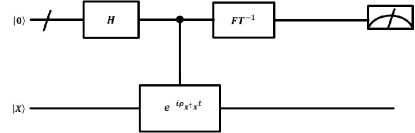
Figure 2: Schematic of the overall phase estimation procedure. The top multiple qubits are the first register(the ’/’ usually denote a bundle of wires), and the bottom qubits are second register. The $FT^{-1}$ refers to the quantum Fourier transformation.

Step (3) Adding an ancilla qubit $\left|0\right\rangle_{6}$, then rotating it from $\left|0\right\rangle_{6}$ to $\sqrt{1-\left({\frac{{C_{1}}}{{\lambda_{r}^{2}+\alpha}}}\right)^{2}}\left|0\right\rangle_{6}+\frac{{C_{1}}}{{\lambda_{r}^{2}+\alpha}}\left|1\right\rangle_{6}$ conditioned by $\left|{\lambda_{r}^{2}}\right\rangle_{5}$. In this way, we can obtain

$$\begin{split}\left|{\varphi_{3}}\right\rangle_{3456}=&\sum\nolimits_{r=1}^{R}{\lambda_{r}}\left|{\vec{u}_{r}}\right\rangle_{3}\left|{\vec{v}_{r}}\right\rangle_{4}\left|{\lambda_{r}^{2}}\right\rangle_{5}\\ &\left({\sqrt{1-\left({\frac{{C_{1}}}{{\lambda_{r}^{2}+\alpha}}}\right)^{2}}\left|0\right\rangle_{6}+\frac{{C_{1}}}{{\lambda_{r}^{2}+\alpha}}\left|1\right\rangle_{6}}\right),\end{split}$$ (20)

where the constant ${C_{1}}$ is chosen to be $O\left({\max\left({\frac{{\lambda_{r}}}{{\lambda_{r}^{2}+\alpha}}}\right)}\right)^{-1}$ that makes $\frac{{C_{1}}}{{\lambda_{r}^{2}+\alpha}}$ as close to 1 as possible while less than 1. The $\alpha$ satisfying $\left[{\Theta\left({\frac{1}{{\kappa^{2}}}}\right),\Theta\left(1\right)}\right]$ (it’s explained later). Then, after performing quantum inverse phase estimation algorithm and discarding the third register $\left|{\lambda_{r}^{2}}\right\rangle_{3}$, the remainder particles are in the state

$$\begin{split}\left|{\varphi_{4}}\right\rangle_{346}=&\sum\nolimits_{r=1}^{R}{\lambda_{r}}\left|{\vec{u}_{r}}\right\rangle_{3}\left|{\vec{v}_{r}}\right\rangle_{4}\\ &\left({\sqrt{1-\left({\frac{{C_{1}}}{{\lambda_{r}^{2}+\alpha}}}\right)^{2}}\left|0\right\rangle_{6}+\frac{{C_{1}}}{{\lambda_{r}^{2}+\alpha}}\left|1\right\rangle_{6}}\right).\end{split}$$ (21)

Step (4) A projection measurement is performed on the ancilla qubit in the basis $\left\{{\left|0\right\rangle,\left|1\right\rangle}\right\}$. Then the probability of obtaining measurement outcome ${\left|1\right\rangle_{6}}$ is $p\left(1\right)=\sum\limits_{r=1}^{R}{\lambda_{r}^{2}\frac{{{C_{1}}^{2}}}{{{{\left({\lambda_{r}^{2}+\alpha}\right)}^{2}}}}}$, from $\frac{{C_{1}}}{{\lambda_{r}^{2}+\alpha}}=\Omega\left({\frac{1}{\kappa}}\right)$, we can derive $p\left(1\right)=O\left({\frac{1}{{{k^{4}}}}}\right)$. After the measurement, the remainder system is in the state

$$\left|{\varphi_{5}}\right\rangle_{34}=\frac{{\sum\limits_{r=1}^{R}{{\lambda_{r}}}\left|{{\vec{u}_{r}}}\right\rangle_{3}\left|{{\vec{v}_{r}}}\right\rangle_{4}\frac{{{C_{1}}}}{{\lambda_{r}^{2}+\alpha}}}}{{\sqrt{p\left(1\right)}}}.$$ (22)

Step (5) The aim of the last step is to obtain the desired result. According to the $\left|{\varphi_{5}}\right\rangle_{34}$, $\left|{{\vec{y}}}\right\rangle_{1}$ and $\left|{\vec{x}^{\prime}}\right\rangle_{2}$, we can get predictive output ${y^{\prime}}$ by the following procedures. First, we need to express the desired result in quantum states in order to make the calculation clearer

$$y^{\prime}=\sum\limits_{r=1}^{R}{\sigma_{r}\left\langle{{\vec{u}_{r}}}\mathrel{\left|{\vphantom{{u_{r}}y}}\right.\kern-1.2pt}\vec{y}\right\rangle\left\langle{{\vec{v}_{r}}}\mathrel{\left|{\vphantom{{\vec{v}_{r}}{\vec{x}^{\prime}}}}\right.\kern-1.2pt}{{\vec{x}^{\prime}}}\right\rangle}.$$ (23)

Secondly, observing state (23) and defining $\left|{\varphi}\right\rangle_{12}=\left|\vec{y}\right\rangle_{1}\left|{\vec{x}^{\prime}}\right\rangle_{2}$ according to Eq. (6) and Eq. (7). The result of performing inner product on $\left|{\varphi_{5}}\right\rangle_{34}$ and $\left|{\varphi_{6}}\right\rangle_{12}$ is in direct proportion to our desired outcome by a Swap Test[17, 18], which is performing Hadamard transform on ancilla qubit ${\left|0\right\rangle_{0}}$, then executing swap operation on $\left|{\varphi_{5}}\right\rangle_{34}$ and $\left|{\varphi_{6}}\right\rangle_{12}$ when the ancilla qubit is ${\left|1\right\rangle}$, followed by measurement on the ancilla qubit in the basis $\left\{{\left|0\right\rangle,\left|1\right\rangle}\right\}$. But the direct operation will result in the probability of success is $\frac{1}{2}+\frac{1}{2}\left|{\left\langle{{\varphi_{5}}}\mathrel{\left|{\vphantom{{\varphi_{5}}{\varphi_{6}}}}\right.\kern-1.2pt}{{\varphi_{6}}}\right\rangle}\right|^{2}$, it is easy to see that the sign of ${\left\langle{{\varphi_{5}}}\mathrel{\left|{\vphantom{{\varphi_{5}}{\varphi_{6}}}}\right.\kern-1.2pt}{{\varphi_{6}}}\right\rangle}$ is ambiguous. Therefore, there is a more deliberate way can avoid the terrible situation: Conditionally preparing these two states to make them entangle with ancilla qubit[19], that is $\frac{{\left|0\right\rangle_{0}\left|{\varphi_{5}}\right\rangle_{34}+\left|1\right\rangle_{0}\left|{\varphi_{6}}\right\rangle_{12}}}{{\sqrt{2}}}$ and then performing the Swap Test on the ancilla qubit with $\frac{{\left|0\right\rangle-\left|1\right\rangle}}{{\sqrt{2}}}$. The probability of success is $Pr=\frac{1}{4}+\frac{1}{4}\left\langle{{\varphi_{5}}}\mathrel{\left|{\vphantom{{\varphi_{5}}{\varphi_{6}}}}\right.\kern-1.2pt}{{\varphi_{6}}}\right\rangle$ that can lead to reveal sign. The circuit of changed Swap Test is given in Fig. 3. In practice, a good RR model make predictive value as close as possible real value ${y_{i}}$, thus the sum of inner product always positive in this case.

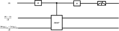
Figure 3: The quantum circuit for the changed Swap Test. The H is Hadamard operation and SWAP is swap operation.

3.2 Algorithm 2: finding an optimal $\alpha$

3.2.1 The specific steps of algorithm 2

According to reference[11,18], we know that a good $\alpha$ can make RR model achieve the best (or approximately best) predictive performance. So, it is of great significance to choose a good $\alpha$.

For RR model, the reference[11] proposed that too large $\alpha$ will make the optimal fitting parameters $\vec{w}$ approach zero which leads to deviate real value and too small $\alpha$ will make the RR reduced to the OLR. Thus, we choose $\alpha$ satisfying $\left[{\Theta\left({\frac{1}{{\kappa^{2}}}}\right),\Theta\left(1\right)}\right]$ based on range of the singular value $\lambda_{r}$. That is to say, ${\alpha_{j}}={\alpha_{min}}+\frac{{\left({j-1}\right)\left({{\alpha_{max}}-{\alpha_{min}}}\right)}}{{L-1}}$ for $j=1,\dots,L$. The common way to get an appropriate $\alpha$ is to choose the best one out of a number of candidates $\alpha^{\prime}$ . The goal of the following steps is to find an appropriate $\alpha$ that give rise to a RR model can well constructed.

For every given input $\vec{x}_{i}$, we will get a predictive value ${y_{i}}^{\prime}$. However, there exist the squared residual sum between predictive values and real values. The predictive values are related to $\alpha$, so we hope that we can find an optimal $\alpha$ to obtain minimum of the squared residual sum. In the algorithm 1, our algorithm only can obtain an output value every time. So, the efficiency is low if we want to input whole training dataset X. Therefore, we propose another subalgorithm that can calculate training dataset X in parallel.

Here, we write ${X}$ in the reduced singular value decomposition form and combine it with Eq. (5), then, we can get a set of column vectors corresponds to M outputs. Where the desired quantum state form $\vec{y}^{\prime}$ is

$$\left|{\vec{x}^{\prime}}\right\rangle_{1}=\sum\limits_{r=1}^{R}{\frac{{\lambda_{r}^{2}}}{{\lambda_{r}^{2}+\alpha}}}\left\langle{{{\vec{u}_{r}}}}\mathrel{\left|{\vphantom{{{\vec{u}_{r}}}y}}\right.\kern-1.2pt}{\vec{y}}\right\rangle\left|{{\vec{u}_{r}}}\right\rangle_{1}.$$ (24)

The details of the second algorithm are described in the following steps and the schematic circuit is given in Fig. 4.

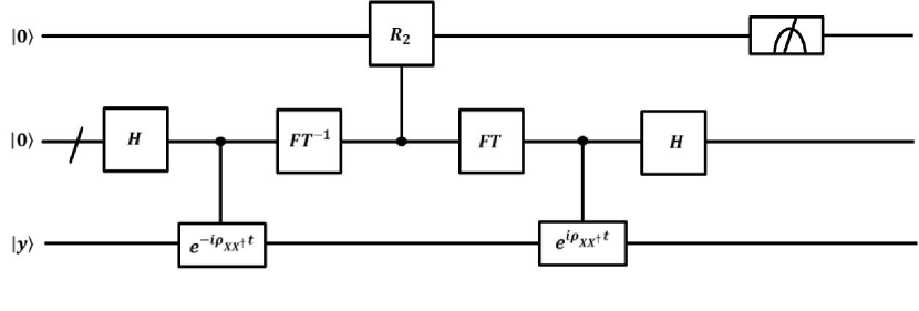
Figure 4: The whole quantum circuit for algorithm 2. Here the ’/’ usually denote a bundle of wires, $H$ refers to Hadamard operation. The $FT$ means quantum Fourier transformation and $FT^{-1}$ denotes the quantum inverse Fourier transformation. The $R_{2}$ is controlled rotation of Step (3).

Step (1) Similar to the algorithm 1, fisrtly preparing initial quantum state of $\vec{y}$, $\vec{x}^{\prime}$ and X which can be efficiently generated as shown in Step (1) of algorithm 1. Next, taking advantage of the Gram-Schmidt decomposition to write $\left|{X}\right\rangle_{34}=\sum\limits_{r=1}^{R}{{\lambda_{r}}}\left|{{\vec{u}_{r}}}\right\rangle_{3}\left|{{\vec{v}_{r}}}\right\rangle_{4}$.

Step (2) Observing Eq. (24), we need to estimate the singular value ${\lambda_{r}^{2}}$ of ${{X}{{X}^{\dagger}}}$. Next, adopting trick of reference[16] to use q copies of ${\rho_{{X}{{X}^{\dagger}}}}$ to apply the unitary operator $e^{i\rho_{{X}{{X}^{\dagger}}}t}$, which allows us to exponentiate a non-sparse but low-rank $M\times M$ - dimension density matrices, where ${\rho_{{X}{{X}^{\dagger}}}}$ is presented in algorithm 1. Followed by performing the quantum phase estimation algorithm on $\left|\vec{y}\right\rangle_{1}$ that lead to obtain

$$\left|{\phi_{1}}\right\rangle_{12}=\sum\nolimits_{r=1}^{R}{\left\langle{{\vec{u}_{r}}}\mathrel{\left|{\vphantom{{\vec{u}_{r}}y}}\right.\kern-1.2pt}{\vec{y}}\right\rangle}\left|{\vec{u}_{r}}\right\rangle_{1}\left|{\lambda_{r}^{2}}\right\rangle_{2}.$$ (25)

The procedures of the phase estimation are same as counterpart of algorithm 1. Just the objective of application by ${\rho_{{X}{{X}^{\dagger}}}}$ is from $\left|{X}\right\rangle_{34}$ to $\left|\vec{y}\right\rangle_{1}$.

Step (3) Adding an ancilla qubit $\left|0\right\rangle_{3}$, then rotating it from $\left|0\right\rangle_{3}$ to $\sqrt{1-\left({\frac{{C_{2}\lambda_{r}^{2}}}{{\lambda_{r}^{2}+\alpha}}}\right)^{2}}\left|0\right\rangle_{3}+\frac{{C_{2}\lambda_{r}^{2}}}{{\lambda_{r}^{2}+\alpha}}\left|1\right\rangle_{3}$ conditioned on ${\left|{\lambda_{r}^{2}}\right\rangle_{2}}$. In this way, we can obtain

$$\begin{split}\left|{\phi_{2}}\right\rangle_{123}=&\sum\nolimits_{r=1}^{R}{\left\langle{{\vec{u}_{r}}}\mathrel{\left|{\vphantom{{\vec{u}_{r}}\vec{y}}}\right.\kern-1.2pt}\vec{y}\right\rangle}\left|{\vec{u}_{r}}\right\rangle_{1}\left|{\lambda_{r}^{2}}\right\rangle_{2}\\ &\left[{\sqrt{1-\left({\frac{{C_{2}\lambda_{r}^{2}}}{{\lambda_{r}^{2}+\alpha}}}\right)^{2}}\left|0\right\rangle_{3}+\frac{{C_{2}\lambda_{r}^{2}}}{{\lambda_{r}^{2}+\alpha}}\left|1\right\rangle_{3}}\right],\end{split}$$ (26)

where the constant ${C_{2}}$ is chosen to be $O\left(1\right)$ for ensuring that amplitude as close as possible to 1 but less than 1. In the next moment, performing the the quantum inverse phase estimation algorithm and discarding the eigenvalue register $\left|{\lambda_{r}^{2}}\right\rangle_{2}$. After these operations, the remainder system is in the state

$$\begin{split}\left|{\phi_{3}}\right\rangle_{13}=&\sum\nolimits_{r=1}^{R}{\left\langle{{\vec{u}_{r}}}\mathrel{\left|{\vphantom{{\vec{u}_{r}}\vec{y}}}\right.\kern-1.2pt}\vec{y}\right\rangle}\left|{\vec{u}_{r}}\right\rangle_{1}\\ &\left[{\sqrt{1-\left({\frac{{C_{2}\lambda_{r}^{2}}}{{\lambda_{r}^{2}+\alpha}}}\right)^{2}}\left|0\right\rangle_{3}+\frac{{C_{2}\lambda_{r}^{2}}}{{\lambda_{r}^{2}+\alpha}}\left|1\right\rangle_{3}}\right].\end{split}$$ (27)

Step (4) Performing conditional measurement on the ancilla qubit in the basis $\left\{{\left|0\right\rangle,\left|1\right\rangle}\right\}$ to get outcome $\left|1\right\rangle_{3}$ and final state after measurement is

$$\left|{\phi_{4}}\right\rangle_{1}=\frac{{\sum\limits_{r=1}^{R}{\frac{{{C_{2}}\lambda_{r}^{2}}}{{\lambda_{r}^{2}+\alpha}}\left\langle{{{\vec{u}_{r}}}}\mathrel{\left|{\vphantom{{{\vec{u}_{r}}}\vec{y}}}\right.\kern-1.2pt}\vec{y}\right\rangle\left|{{\vec{u}_{r}}}\right\rangle_{1}}}}{{\sqrt{p\left(2\right)}}},$$ (28)

with $p\left(2\right)={\left({\sum\limits_{r=1}^{R}{\left\langle{{{\vec{u}_{r}}}}\mathrel{\left|{\vphantom{{{\vec{u}_{r}}}\vec{y}}}\right.\kern-1.2pt}\vec{y}\right\rangle}\frac{{{C_{2}}\lambda_{r}^{2}}}{{\lambda_{r}^{2}+\alpha}}}\right)^{2}}$. It is easy to see that $\left|{\vec{y}^{\prime}}\right\rangle_{1}=\frac{{\sqrt{p(2)}\left|{\phi_{4}}\right\rangle_{1}}}{{{C_{2}}}}$.

Step (5) Given a set of candidates $\left\{{\alpha_{1},...,\alpha_{L}}\right\}$, computing the loss function

$$\begin{split}E\left({\alpha_{l}}\right)&=\left|{\left|{\vec{y}^{\prime}}\right\rangle-\left|\vec{y}\right\rangle_{1}}\right|^{2}\\ &=\left\langle{\vec{y}^{\prime}|{\vec{y}^{\prime}}}\right\rangle+\left\langle{\vec{y}|\vec{y}}\right\rangle-2\left\langle{\vec{y}^{\prime}|\vec{y}}\right\rangle\\ &=\frac{{p\left(2\right)}}{{C_{2}^{2}}}+1-2\frac{{\sqrt{p(2)}}}{{{C_{2}}}}\left\langle{{\phi_{3}}}\mathrel{\left|{\vphantom{{\phi_{4}}y}}\right.\kern-1.2pt}\vec{y}\right\rangle,\end{split}$$ (29)

where $p\left(2\right)$ is probability of measured result and ${C_{2}}$ is a known constant. The step is important, because we want the fitted model to capture the typical relationship among the real values and predictive values so that it can be generalized to new data. This require that we choose an optimal ${\hat{\alpha}}$ that obtain minimum $E\left({\hat{\alpha}}\right)$. For $\left\langle{{\phi_{4}}}\mathrel{\left|{\vphantom{{\phi_{4}}\vec{y}}}\right.\kern-1.2pt}\vec{y}\right\rangle$, we can adopt the Swap Test to obtain the desired consequences.

Step (6) For every $\alpha\in\left\{{\alpha_{1},\alpha_{2},...,\alpha_{L}}\right\}$, executing Steps (1)-(5), then picking out the best $\alpha$ with minimum $E\left(\alpha\right)$ as the final regularization hyperparameter ${\hat{\alpha}}$ for RR. Thus, we will get L results of the loss function by L repetitions of algorithm 2.

4 Runtime analysis of algorithm

4.1 Runtime analysis of algorithm 1

Density matrix exponentiation is a powerful tool to analyze the properties of unknown density matrices. According to[16], one needs time resource $O\left({{\varepsilon^{-3}}}\right)$ copies of ${\rho_{{X}{{X}^{\dagger}}}}$ to apply the unitary operator ${e^{-i\;{\rho_{{X}{{X}^{\dagger}}}}t}}$, which allows accuracy $\varepsilon=O\left({{{{t^{2}}}\mathord{\left/{\vphantom{{{t^{2}}}q}}\right.\kern-1.2pt}q}}\right)$. Therefore, one constructs the eigenvectors and eigenvalues of a low-rank $\left({M\times M}\right)$-dimension matrix ${\rho_{{X}{{X}^{\dagger}}}}$ in time $O\left({\log_{2}M}\right)$. And the runtime complexity of the controlled rotation is $O\left({log\left({\frac{1}{\varepsilon}}\right)}\right)$. Compared with the phase estimation algorithm, the runtime of this step is negligible. The probability of getting predictive value is $p\left(1\right)=O\left({\frac{1}{{{k^{4}}}}}\right)$, which means we need $O\left({{k^{4}}}\right)$ to obtain desired results on average. Amplitude amplification[20,21] reduces this times to $O\left({{k^{2}}}\right)$ in the runtime. The Swap Test routine is also linear in the number of qubits, and the final measurement only accounts for a constant factor. Of course, time complexity on state preparing is $O\left({\log_{2}MN}\right)$. Thus, the upper bound of runtime roughly is $O\left({\kappa^{2}poly\log_{2}\left({MN}\right)\varepsilon^{-3}}\right)$. Comparisons of time complexity between classical counterpart, Liu and Zhang’s quantum algorithm, Yu’s improved quantum algorithm and our proposed quantum algorithm are detailed in TABLE1.

TABLE I: Comparisons of time complexity about algorithm 1

Algorithm	Time Complexity
Classical counterpart	$O\left({MN+{{N^{2}R\log\left({\frac{R}{\varepsilon}}\right)}\mathord{\left/{\vphantom{{N^{2}R\log\left({\frac{R}{\varepsilon}}\right)}{\varepsilon^{2}}}}\right.\kern-1.2pt}{\varepsilon^{2}}}}\right)$
Liu’s algorithm	$O\left({\log_{2}\left({M+N}\right){{s^{2}\kappa_{R}^{3}}\mathord{\left/{\vphantom{{s^{2}\kappa_{R}^{3}}{\varepsilon^{2}}}}\right.\kern-1.2pt}{\varepsilon^{2}}}}\right)$
Yu’s algorithm	$O\left({\left\|{X}\right\|_{\max}^{2}poly\log_{2}\left({M+N}\right){{\kappa^{3}}\mathord{\left/{\vphantom{{\kappa^{3}}{\varepsilon^{3}}}}\right.\kern-1.2pt}{\varepsilon^{3}}}}\right)$
Our algorithm	$O\left({{{\kappa^{2}\log M}\mathord{\left/{\vphantom{{\kappa^{2}\log_{2}M}{\varepsilon^{3}}}}\right.\kern-1.2pt}{\varepsilon^{3}}}}\right)$

From above TABLE 1, we have an exponential speedup on MN when compared with result of the best classical counterpart, whereas the dependence on accuracy of a factor $\varepsilon$ that is small. So our algorithm 1 is accelerated totally. What’s more, there are slightly advantage when compared our algorithm with similar quantum algorithm. Because Liu and Yu didn’t take state preparing into account, our time complexity is $O\left({{{\kappa^{2}\log_{2}M}\mathord{\left/{\vphantom{{\kappa^{2}\log M}{\varepsilon^{3}}}}\right.\kern-1.2pt}{\varepsilon^{3}}}}\right)$ when we discard time complexity of state preparing. Frist, Liu’s quantum RR algorithm, whose time complexity is $O\left({\log_{2}\left({M+N}\right){{s^{2}\kappa_{R}^{3}}\mathord{\left/{\vphantom{{s^{2}\kappa_{R}^{3}}{\varepsilon^{2}}}}\right.\kern-1.2pt}{\varepsilon^{2}}}}\right)$, where s is the sparsity of the matrix, the dependence on conditional number $\kappa$ is slightly better than his algorithm, whereas dependence on $\varepsilon$ is slightly worse. Secondly, our algorithm can deal with the non-sparse matrix. And runtime of Yu’s quantum RR is $O\left({\left\|{X}\right\|_{\max}^{2}poly\log_{2}\left({M+N}\right){{\kappa^{3}}\mathord{\left/{\vphantom{{\kappa^{3}}{\varepsilon^{3}}}}\right.\kern-1.2pt}{\varepsilon^{3}}}}\right)$ when the matrix is low-rank. So we have a little advantages about depending on conditional number $\kappa$, and have same dependence on $\varepsilon$ as Yu’ result.

4.2 Runtime analysis of algorithm 2

Time complexity of algorithm 2 is similar to algorithm 1, just the probability of measurement is $p\left(2\right)$, which means we need $\frac{1}{{p\left(2\right)}}$ to obtain desired results on average. Amplitude amplification reduces this times to $\frac{1}{{\sqrt{p(2)}}}$ in the runtime. Here, ${\left|{{\vec{u}_{r}}}\right\rangle}$ are quantum states representing the orthogonal sets of left eigenvectors of ${X}$. Adding another ${M-R}$ normalized vectors $\left|{{\vec{u}_{R+1}}}\right\rangle,\ldots,\left|{{\vec{u}_{M}}}\right\rangle$ that make $\left|{{\vec{u}_{1}}}\right\rangle,\ldots,\left|{{\vec{u}_{M}}}\right\rangle$ become an orthonormal basis in whole space ${R^{M}}$. Therefore, $\left|\vec{y}\right\rangle$ can be written as a linear combination of $\left\{{\left.{\left|{{\vec{u}_{\rm{r}}}}\right\rangle}\right\}}\right._{1}^{M}$, that is $\left|\vec{y}\right\rangle_{2}=\sum\limits_{r=1}^{N}{\left\langle{{\vec{u}_{r}}|\vec{y}}\right\rangle}\left|{{\vec{u}_{\rm{r}}}}\right\rangle_{2}$ with $\sum\limits_{r=1}^{N}{{{\left\langle{{\vec{u}_{\rm{r}}}|\vec{y}}\right\rangle}^{2}}}=1$. According to[11], we know that $\sum\limits_{r=1}^{R}{{{\left\langle{{\vec{u}_{\rm{r}}}|\vec{y}}\right\rangle}^{2}}}$ should be closed to 1. So $p\left(2\right)={\left({\sum\limits_{r=1}^{R}{\left\langle{{{\vec{u}_{r}}}}\mathrel{\left|{\vphantom{{{u_{r}}}\vec{y}}}\right.\kern-1.2pt}\vec{y}\right\rangle}\frac{{{C_{2}}\lambda_{r}^{2}}}{{\lambda_{r}^{2}+\alpha}}}\right)^{2}}\leq O\left(1\right)$, which means we need less than $O\left(1\right)$ to obtain desired results on average. For L $\alpha$, we have to perform algorithm 2 L to get all results at once. Thus, the upper bound of runtime roughly is $O\left({Lpoly\log_{2}M\varepsilon^{-3}}\right)$. Compared with classical counterpart, we have an exponential speedup of factors M and N, whereas have slightly worse the dependence on error of a factor $\varepsilon$. Even so, our algorithm 2 have a speedup totally. In addition, there is slightly better than Yu’s improved quantum algorithm when we take same behaviour that don’t take state preparing into account. Details are shown in the TABLE 2 above.

TABLE II: Comparisons of time complexity about algorithm 2

Algorithm	Time Complexity
Classical counterpart	$O\left({LMN+\frac{{LN^{2}\left({\sum\nolimits_{l=1}^{K}{R_{l}\log\left({\frac{R}{\varepsilon}}\right)}}\right)}}{{\varepsilon^{2}}}}\right)$
Yu’s algorithm	$O\left({\frac{{L\left\|{X}\right\|_{\max}^{2}poly\log_{2}\left({M+N}\right)\kappa^{\prime 4}\kappa}}{{\varepsilon^{4}}}}\right)$
Our algorithm	$O\left({{{L\log_{2}M}\mathord{\left/{\vphantom{{L\log_{2}M}{\varepsilon^{3}}}}\right.\kern-1.2pt}{\varepsilon^{3}}}}\right)$

As you can see from the above TABLE 2, compared with the classical counterpart, we have an exponential speedup of a factor $M$, whereas the dependence on accuracy of a factor $\varepsilon$. Liu’s algorithm doesn’t determine a good $\alpha$, so our algorithm 2 is unnecessary to compare. In addition, we are better than Yu’s improved quantum algorithm about dependence on error $\varepsilon$ and condition number $\kappa$.

4.3 The whole quantum algorithm for RR

In the paper, we address RR model in quantum setting, which is one of the significant problems in data prediction. In particular, the algorithm starts with algorithm 2 to find an appropriate regularization hyperparameter $\alpha$, then we plug $\alpha$ into algorithm 1 to present a procedure that can further used to efficiently predict an output ${y^{\prime}}$ for the new input $\vec{x}^{\prime}$.

The whole time complexity is $O\left({\left({\kappa^{2}+L}\right)\log_{2}M\varepsilon^{-3}}\right)$, which has an exponential speedup over classical counterpart.

5 Conclusion

In general, we have presented a quantum algorithm that can efficiently perform quantum ridge regression over a large dataset in age of big data. Firstly, we described an quantum algorithm 1 that can predict outputs for new different input ${\vec{x}^{\prime}}$. Secondly, we present a quantum algorithm to find a good regularization hyperparameter $\alpha$. The whole algorithm begins with algorithm 2. It is shown that algorithm can address non-sparse matrices and have an exponential speedup over classical algorithm when the matrix is low-rank. Of course, there is a limitation to some certain that our algorithm only effectively tackle low-rank matrices and have slight speedup when rank of matrix is high [23].

At present, since the application of machine learning is more and more extensive and quantum algorithm is also very promising, the proposal of quantum machine learning is a very significant progress but challenging. We hope that the idea of this algorithm can be applied to other fields of information technology[24-32] to explore better possibilities in the future. What’s more, we believe that even though the field of quantum machine learning is still in an early stage of development, it will eventually an become increasingly mature field.

References

- [1] M. Schuld, I. Sinayskiy and F. Petruccione, An introduction to quantum machine learning, Contemporary Physics 56, 2 (2015).
- [2] J. Biamonte, P. Wittek and N. Pancotti, Quantum Machine Learning, Nature 549, 195 (2017).
- [3] H Chen, R. H Chiang, V. C Storey, Business intelligence and analytics: from big data to big impact. Management Information Systems Quarterly, 36, 4 (2012).
- [4] P. Walther, K. J. Resch and T. Rudolph, Experimental One-Way Quantum Computing, Nature 434, 169 (2005).
- [5] A. D. Alhaidari and T. J. Taiwo, Wilson-Racah quantum system, Journal of Mathematical Physics 58, 022101 (2017).
- [6] P. W. Shor, Algorithms for quantum computation: discrete logarithms and factoring, In Proceedings 35th Annual Symposium on Foundations of Computer Science, 124 (1994).
- [7] N. Wiebe, D. Braun and S. Lloyd, Quantum algorithm for data fitting, Physical Review Letters 109, 050505 (2012).
- [8] A. W. Harrow, A. Hassidim, S. Lloyd, Quantum Algorithm for Linear Systems of Equations, Physical Review Letters 15, 150502 (2009).
- [9] M. Schuld, I. Sinayskiy and F. Petruccione, Prediction by linear regression on a quantum computer, Physical Review A 94, 022342 (2016).
- [10] Y. Liu and S. Zhang, Fast quantum algorithms for least squares regression and statistic leverage scores, Theoretical Computer Science 657, 38 (2017).
- [11] C. H. Yu, F. Gao and Q. Y. Wen, An improved quantum algorithm for ridge regression, IEEE Transactions on Knowledge and Data Engineering, 1, 1 (2019).
- [12] A. E.Hoerl and R. W.Kennard, Ridge regression: biased estimation for nonorthogonal problems, Technometrics 42, 80 (2000).
- [13] D. Lay, Handbook of Linear Algebra, Discrete Mathematics and Its Applications, Chapman and Hall/CRC (2014).
- [14] C. H. Yu, F. Gao and C. H. Liu, Quantum algorithm for visual tracking, Physical Review A 99, 022301 (2019).
- [15] M. A.Nielsen and I. L.Chuang, Quantum computation and quantum information (Cambridge university press, 2010).
- [16] S. Lloyd , M. Mohseni and P. Rebentrost, Quantum principal component analysis, Nature Physics 10, 631(2014).
- [17] H. Buhrman, R. Cleve and J. Watrous, Quantum fingerprinting, Physical Review Letters 87, 167902 (2001).
- [18] S. Lloyd, M. Mohseni and P. Rebentrost, Quantum algorithms for supervised and unsupervised machine learning, arXiv: 1307.0411 (2013).
- [19] P. Rebentrost, M. Mohseni and S. Lloyd, Quantum Support Vector Machine for Big Data Classification, Physical Review A 113, 130503 (2014).
- [20] G. Brassard, P. Hoyer and M. Mosca, Quantum Amplitude Amplification and Estimation, arXiv: quant-ph/0005055 (2000).
- [21] A. E. Rastegin, On the role of dealing with quantum coherence in amplitude amplification, Quantum Information Processing 17, 179 (2018).
- [22] V. Wieringen and N. Wessel, Lecture notes on ridge regression, arXiv:1509.09169 (2015).
- [23] P. Rebentrost, A. Steffens, I. Marvian and S. Lloyd, Quantum singular-value decomposition of nonsparse low-rank matrices, Physical Review A 97, 012327 (2018).
- [24] N. Wiebe, A. Kapoor and K. M. Svore, Quantum algorithms for nearest-neighbor methods for supervised and unsupervised learning, Quantum Information and Computation 15, 316 (2015).
- [25] D. W.Berry, G. Ahokas and R. Cleve, Efficient Quantum Algorithms for Simulating Sparse Hamiltonians, Communications in Mathematical Physics 270, 359 (2007).
- [26] I. Cong and L. M. Duan, Quantum discriminant analysis for dimensionality reduction and classification, New Journal of Physics 18, 073011 (2016).
- [27] Y. Ruan, X. Xue and H. Liu, Quantum Algorithm for K-Nearest Neighbors Classification Based on the Metric of Hamming Distance, International Journal of Theoretical Physics 56, 3496 (2017).
- [28] G. D. Paparo, M. Muller and F. Comellas, Quantum Google in a Complex Network, Scientific Reports 3, 2773 (2013).
- [29] M. Schuld and i. P. Sinayskiy, The quest for a Quantum Neural Network, Quantum Information Process 13, 2567 (2012).
- [30] L. Grover and T. Rudolpha, Creating superpositions that correspond to efficiently integrable probability distributions, arXiv: quant-ph/0208112 (2002).
- [31] P. Kaye and M. Mosca, Quantum Networks for Generating Arbitrary Quantum States, arXiv: quant-ph/0407102 (2001).
- [32] A. N. Soklakov and R. Schack, Repeat-until-success quantum computing using stationary and flying qubits, Physical Review A 73, 012307 (2006).