On the Evaluation of the Eigendecomposition of the Airy Integral Operator

Zewen Shen$\mbox{}^{\dagger\,\star}$ and Kirill Serkh$\mbox{}^{\ddagger\,\diamond}$

v4, updated June 17, 2022

$\mbox{}^{\diamond}$ This author’s work was supported in part by the NSERC Discovery Grants RGPIN-2020-06022 and DGECR-2020-00356.

$\mbox{}^{\dagger}$ Dept. of Computer Science, University of Toronto, Toronto, ON M5S 2E4
$\mbox{}^{\ddagger}$ Dept. of Math. and Computer Science, University of Toronto, Toronto, ON M5S 2E4

$\mbox{}^{\star}$ Corresponding author

1 Introduction

Recently, random matrix theory (RMT) has become one of the most exciting fields in probability theory, and has been applied to problems in physics [14], high-dimensional statistics [24], wireless communications [8], finance [5], etc. The Tracy-Widom distributions, or, more generally, the distributions of the $k$-th largest level at the soft edge scaling limit of Gaussian ensembles, are some of the most important distributions in RMT, and their numerical evaluation is a subject of great practical importance (see [19, 11] for friendly introductions to RMT, and see [3] for an overview of the numerical aspects of RMT). There are generally two ways of calculating the distributions to high accuracy numerically: one, using the Painlevé representation of the distribution to reduce the calculation to solving a nonlinear ordinary differential equation (ODE) numerically [10], and the other, using the determinantal representation of the distribution to reduce the calculation to an eigenproblem involving an integral operator [3].

In the celebrated work [30], the Tracy-Widom distribution for the Gaussian unitary ensemble (GUE) was shown to be representable as an integral of a solution to a certain nonlinear ODE called the Painlevé II equation. This nonlinear ODE can be solved to relative accuracy numerically, but achieving relative accuracy is extremely expensive, since it generally requires multi-precision arithmetic [25]. In addition, the extension of the ODE approach to the computation of the $k$-th largest level at the soft edge scaling limit of Gaussian ensembles is not straightforward, as it requires deep analytic knowledge for deriving connection formulas [3, 10].

On the other hand, the method based on the Fredholm determinantal representation uses the fact that the cumulative distribution function (CDF) of the $k$-th largest level at the soft edge scaling limit of the Gaussian unitary ensemble can be written in the following form:

$$F_{2}(k;s)=\sum_{j=0}^{k-1}\frac{(-1)^{j}}{j!}\frac{\partial^{j}}{\partial z^{j}}\det\big{(}I-z\mathcal{K}|_{L^{2}[s,\infty)}\big{)}\Bigr{|}_{z=1},$$ (1)

where $\mathcal{K}|_{L^{2}[s,\infty)}$ denotes the integral operator on $L^{2}[s,\infty)$ with kernel

$$K_{Ai}(x,y)=\int_{s}^{\infty}\text{Ai}(x+z-s)\text{Ai}(z+y-s)\,\mathrm{d}z,$$ (2)

where $\text{Ai}(x)$ is the Airy function of the first kind (see [30, 13] for the derivations). We also note that there exist similar Fredholm determinantal representations for the cases of the Gaussian orthogonal ensemble (GOE) and Gaussian sympletic ensemble (GSE) (see Section 5.1). The cumulative distribution function and the probability density function (PDF) of the distribution can be computed using the eigendecomposition of the so-called Airy integral operator $\mathcal{T}_{s}$, where $\mathcal{T}_{s}[f](x)=\int_{0}^{\infty}\text{Ai}(x+y+s)f(y)\,\mathrm{d}y$ for $x\geq 0$. This is because $\mathcal{K}|_{L^{2}[s,\infty)}=\mathcal{G}_{s}^{2}$, where $\mathcal{G}_{s}[f](x)=\int_{s}^{\infty}\text{Ai}(x+y-s)f(y)\,\mathrm{d}y$ for $x\geq s$, and $\mathcal{T}_{s}$ shares the same eigenvalues and eigenfunctions (up to a translation) with $\mathcal{G}_{s}$. If the eigenvalues of the integral operator $\mathcal{T}_{s}$ are computed directly, they can be known only to absolute precision, since $\mathcal{T}_{s}$ is a compact integral operator. Furthermore, the number of degrees of freedom required to discretize $\mathcal{T}_{s}$ increases when the kernel is oscillatory (as $s\to-\infty$).

In this paper, we present a new method for computing the eigendecomposition of the Airy integral operator $\mathcal{T}_{s}$, which solves an open problem in random matrix theory (see, for example, Open Problem 6 in [9]). It exploits the remarkable fact that the Airy integral operator admits a commuting differential operator, which shares the same eigenfunctions (see, for example, [30, 16]). In our method, we compute the spectrum and the eigenfunctions of the differential operator by computing the eigenvalues and eigenvectors of a banded eigenproblem. Since the eigenproblem is banded, the eigendecomposition can be done very quickly in $\mathcal{O}(n^{2})$ operations, and the eigenvalues and eigenvectors can be computed to entry-wise full relative precision. Finally, we use the computed eigenfunctions to recover the spectrum of the Airy integral operator $\mathcal{T}_{s}$, also to full relative precision.

As a direct application, our method computes the distributions of the $k$-th largest level at the soft edge scaling limit of Gaussian ensembles to full relative precision rapidly everywhere, except in the left tail (the left tail is computed to absolute precision). We note that several other integral operators admitting commuting differential operators have been studied numerically from the same point of view as this paper (see, for example, [23, 18])

Integral operators like $\mathcal{T}_{s}$, which admit commuting differential operators, are known as bispectral operators (see, for example, [6]). One famous example of a bispectral operator is the truncated Fourier transform, which was investigated by Slepian and his collaborators in the 60’s [29]; its eigenfunctions are known as prolate spheroidal wavefunctions. We note that, unlike prolates, the eigenfunctions of the operator $\mathcal{T}_{s}$ are relatively unexamined: “The behavior of the eigenfunctions, a problem of great practical interest, presents a serious numerical challenge” (see Open Problem 6 in [9]); “In the case of the Airy kernel, the differential equation did not receive much attention and its solutions are not known” (see Section 24.2 in [21]). In this paper, we also characterize these previously unstudied eigenfunctions, and describe their extremal properties in relation to an uncertainty principle involving the Airy transform.

Finally, we note that the Airy integral operator $\mathcal{T}_{s}$ is rather universal. For example, in Section 5.2, we describe an application to optics. In that section, we use the eigenfunctions of the Airy integral operator to compute finite-energy Airy beams that are optimal, in the sense that they maximally concentrate energy near the main lobes in their initial profiles, while also remaining diffraction-free over the longest possible distances.

2 Mathematical and Numerical Preliminaries

In this section, we introduce the necessary mathematical and numerical preliminaries.

2.1 Airy function of the first kind

The Airy function of the first kind is the solution to the differential equation

$$\frac{d^{2}f}{dx^{2}}-xf=0,$$ (3)

for all $x\in\mathbbm{R}$, that decays for large $x$. It can also be written in an integral representation

$$\text{Ai}(x)=\frac{1}{\pi}\int_{0}^{\infty}\cos\Bigl{(}\frac{t^{3}}{3}+xt\Bigr{)}\,\mathrm{d}t.$$ (4)

Remark 2.1.

One can extend the definition of $\text{Ai}(x)$ to the complex plane and show that it is an entire function.

Remark 2.2.

As $x\to+\infty$,

$$\text{Ai}(x)\sim\frac{e^{-\frac{2}{3}x^{3/2}}}{2\pi^{1/2}x^{1/4}}.$$ (5)

2.2 The Airy Integral Operator

In this section, we give the definition and properties of the Airy integral operator.

2.2.1 The Airy integral operator $\mathcal{T}_{c}$ and its associated integral operator $\mathcal{G}_{c}$

In this subsection, we define the Airy integral operator, including its eigenvalues and eigenfunctions. Its associated integral operator is introduced as well.

Definition 2.1.

Given a real number $c$, let $\mathcal{T}_{c}\colon L^{2}[0,\infty)\to L^{2}[0,\infty)$ denote the Airy integral operator defined by

$$\mathcal{T}_{c}[f](x)=\int_{0}^{\infty}\text{Ai}(x+y+c)f(y)\,\mathrm{d}y,\quad x\geq 0.$$ (6)

Let $\mathcal{G}_{c}\colon L^{2}[c,\infty)\to L^{2}[c,\infty)$ denote the associated Airy integral operator defined by

$$\mathcal{G}_{c}[f](x)=\int_{c}^{\infty}\text{Ai}(x+y-c)f(y)\,\mathrm{d}y,\quad x\geq c.$$ (7)

Obviously, $\mathcal{G}_{c}$ and $\mathcal{T}_{c}$ are both compact and self-adjoint.

We denote eigenvalues of $\mathcal{T}_{c}$ by $\lambda_{0,c},\lambda_{1,c},\dots,\lambda_{n,c},\dots$, ordered so that ${\lvert\lambda_{j-1,c}\rvert}\geq{\lvert\lambda_{j,c}\rvert}$ for all $j\in\mathbbm{N}^{+}$. For each non-negative integer $j$, let $\psi_{j,c}$ denote the $(j+1)$-th eigenfunction of $\mathcal{T}_{c}$, so that

$$\lambda_{j,c}\psi_{j,c}(x)= \int_{0}^{\infty}\text{Ai}(x+y+c)\psi_{j,c}(y)\,\mathrm{d}y,\quad x\in[0,\infty).$$ (8)

In this paper, we normalize the eigenfunctions such that ${\lVert\psi_{j,c}\rVert}_{2}=1$ for any real number $c$ and non-negative integer $j$. Since the eigenfunctions are real, this condition only specifies the eigenfunctions up to multiplication by $-1$. We thus require that $\psi_{j,c}(0)>0$ (we show in Theorem A.2 in Appendix A that $\psi_{j,c}(0)\neq 0$).

Note that $\mathcal{T}_{c}$ and $\mathcal{G}_{c}$ share the same eigenvalues and eigenfunctions up to a translation, i.e. $\lambda_{j,c},\psi_{j,c}(x)$ is an eigenpair of the operator $\mathcal{T}_{c}$, and $\lambda_{j,c},\psi_{j,c}(x-c)$ is an eigenpair of the operator $\mathcal{G}_{c}$ (see Theorem 2.2). Note that the operator $\mathcal{T}_{c}$ is more convenient to work with than the operator $\mathcal{G}_{c}$, as its domain is invariant under change of $c$. Therefore, we will mainly focus on the study of the Airy integral operator $\mathcal{T}_{c}$ in this paper.

Remark 2.3.

For simplicity, we will use $\lambda_{j}$ and $\psi_{j}$ to denote the eigenvalue and the eigenfunction when there is no ambiguity.

2.2.2 Properties and connection to the Airy transform

Definition 2.2.

Let $\mathcal{A}\colon L^{2}(\mathbbm{R})\to L^{2}(\mathbbm{R})$ denote the integral transform defined by the formula

$$\mathcal{A}[\phi](x)=\int_{-\infty}^{\infty}\text{Ai}(x+y)\phi(y)\,\mathrm{d}y.$$ (9)

In a mild abuse of terminology, we call $\mathcal{A}$ the Airy transform. Note that the standard Airy transform of $\phi$ is defined as $\int_{-\infty}^{\infty}\text{Ai}(x-y)\phi(y)\,\mathrm{d}y$, which can be written as $\mathcal{A}\circ R$, where $R$ denotes the reflection operator.

It is well-known that $\mathcal{A}$ is unitary, and that $\mathcal{A}^{2}=I$, where $I$ is the identity operator (see, for example, [33]). To introduce the connection between the Airy transform $\mathcal{A}$, the so-called Airy kernel integral operator $\mathcal{K}$ (see formula (2)), and the two integral operators $\mathcal{T}_{c},\mathcal{G}_{c}$ defined in Section 2.2.1, we first define the following operators.

Definition 2.3.

Given real numbers $a$ and $b$, let $F_{a,b}\colon L^{2}(\mathbbm{R})\to L^{2}(\mathbbm{R})$ be the operator defined by the formula

$$F_{a,b}[\phi](x)=\mathbbm{1}_{[b,\infty)}(x)\mathcal{A}[\mathbbm{1}_{[a,\infty)}(y)\phi(y)](x),$$ (10)

where $\mathbbm{1}_{X}$ denotes the indicator function associated with the set $X$. Let $\widetilde{F}_{c}$ be a synonym for the operator $F_{0,c}$.

The operator $F_{a,b}$ represents a truncation or “band-limiting” to the half line $[a,\infty)$, followed by an Airy transform, followed by another truncation to the half line $[b,\infty)$. Clearly, $F_{a,b}^{*}=F_{b,a}$.

Definition 2.4.

Given a real number $c$, let $P_{c}\colon L^{2}(\mathbbm{R})\to L^{2}(\mathbbm{R})$ denote the projection operator defined by the formula

$$P_{c}[\phi](x)=\mathbbm{1}_{[c,\infty)}(x)\phi(x).$$ (11)

It’s easy to see that $\widetilde{F}_{c}=P_{c}\mathcal{A}P_{0}$, and that $\widetilde{F}_{-\infty}=\mathcal{A}P_{0}$.

Definition 2.5.

Given a real number $c$, let $T_{c}\colon L^{2}(\mathbbm{R})\to L^{2}(\mathbbm{R})$ denote the translation operator defined by the formula

$$T_{c}[\phi](x)=\phi(x-c).$$ (12)

Below, we define the integral operator $\mathcal{K}$.

Definition 2.6.

Let $\mathcal{K}\colon L^{2}(\mathbbm{R})\to L^{2}(\mathbbm{R})$ denote the integral operator with kernel

$$K_{\text{Ai}}(x,y)=\int_{0}^{\infty}\text{Ai}(x+z)\text{Ai}(y+z)\,\mathrm{d}z.$$ (13)

Clearly, $\mathcal{K}=\widetilde{F}_{-\infty}\widetilde{F}_{-\infty}^{*}$. Moreover, by a change of variables, the kernel (13) can be rewritten as

$$K_{\text{Ai}}(x,y)=\int_{c}^{\infty}\text{Ai}(x+z-c)\text{Ai}(y+z-c)\,\mathrm{d}z,$$ (14)

from which we see that $\mathcal{K}|_{L^{2}[c,\infty)}$ (equivalently, $P_{c}\mathcal{K}P_{c}$ or $\widetilde{F}_{c}{\widetilde{F}_{c}}^{*}$) is equal to the square of the associated Airy integral operator $\mathcal{G}_{c}$ defined in Definition 2.1. Thus, the eigenfunctions and eigenvalues of $\mathcal{K}|_{L^{2}[c,\infty)}$ are given by $\psi_{j,c}(x-c)$ and $\lambda_{j,c}^{2}$ (see formula (8)), respectively.

The following theorem, proved in Lemma 2 of [30], states that the eigenvalues $\lambda_{j,c}$ approach one in absolute value as $c\to-\infty$.

Theorem 2.1.

For each $j$, $\lambda_{j,c}^{2}\to 1$ as $c\to-\infty$, where $\lambda_{j,c}$ is the $(j+1)$-th eigenvalue of the Airy integral operator $\mathcal{T}_{c}$.

Proof. We first show that $\mathcal{K}$ is a projection operator. Since $\widetilde{F}_{-\infty}=\mathcal{A}P_{0}$, we have that $\mathcal{K}=\widetilde{F}_{-\infty}\widetilde{F}_{-\infty}^{*}=\mathcal{A}P_{0}\mathcal{A}$, so $\mathcal{K}^{2}=\mathcal{A}P_{0}\mathcal{A}^{2}P_{0}\mathcal{A}$. Recalling that $\mathcal{A}^{2}=I$, it follows that $\mathcal{K}^{2}=\mathcal{A}P_{0}\mathcal{A}=\mathcal{K}$. Since $\mathcal{K}$ is a projection, its spectrum takes values in the set $\{0,1\}$, and since $\mathcal{K}$ has an infinite dimensional range, it has infinitely many eigenvalues equal to $1$. The operator $P_{c}\mathcal{K}P_{c}$ converges to $\mathcal{K}$ as $c\to-\infty$, so it follows that, for each $j$, $\lambda_{j,c}^{2}\to 1$ as $c\to-\infty$. $\blacksquare$

In the next theorem, we show that the Airy integral operator $\mathcal{T}_{c}$ is related to its associated integral operator $\mathcal{G}_{c}$ by a similarity transformation.

Theorem 2.2.

The Airy integral operator $\mathcal{T}_{c}$ is similar to its associated integral operator $\mathcal{G}_{c}$. Furthermore, if $\lambda_{j,c}$ and $\psi_{j,c}$ are eigenvalues and eigenfunctions of $\mathcal{T}_{c}$, then $\lambda_{j,c}$ and $\psi_{j,c}(x-c)$ are eigenvalues and eigenfunctions of $\mathcal{G}_{c}$.

Proof. We observe that $\mathcal{T}_{c}=T_{-c}F_{0,c}$, so $\mathcal{T}_{c}=T_{-c}(T_{c}F_{c,0}T_{c})=T_{-c}\mathcal{G}_{c}T_{c}$. Since $T_{c}^{*}=T_{-c}$ and $T_{c}T_{c}^{*}=I$, we see that $\mathcal{T}_{c}$ is related to $\mathcal{G}_{c}$ by a similarity transformation. The statement about the eigenfunctions and eigenvalues follows immediately. $\blacksquare$

Finally, we characterize the relation between the eigenfunction $\psi_{j,c}$ and its Airy transform $\mathcal{A}[\psi_{j,c}]$.

Theorem 2.3.

For any real $c$, there exists an analytic continuation of the eigenfunction $\psi_{j,c}$ of the Airy integral operator with parameter $c$, which we denote by $\widetilde{\psi}_{j,c}$. Furthermore,

$$\widetilde{\psi}_{j,c}(x)=\frac{1}{\lambda_{j,c}}\mathcal{A}[\psi_{j,c}](x+c),$$ (15)

for all $x\in\mathbbm{R}$, where $\lambda_{j,c}$ is the corresponding eigenvalue of $\psi_{j,c}$.

Proof. The existence of the analytic continuation $\psi_{j,c}$ is given by formula (8) and the fact that the Airy function is analytic and decays superexponentially. Note that

$$\mathcal{T}_{c}=T_{-c}F_{0,c}=T_{-c}P_{c}\mathcal{A}=P_{0}T_{-c}\mathcal{A},$$ (16)

so after applying both sides of (16) to $\psi_{j,c}$, we get

$$\lambda_{j,c}\psi_{j,c}(x)=P_{0}\mathcal{A}[\psi_{j,c}](x+c),$$ (17)

from which it follows that

$$\widetilde{\psi}_{j,c}(x)=\frac{1}{\lambda_{j,c}}\mathcal{A}[\psi_{j,c}](x+c),$$ (18)

for all $x\in\mathbbm{R}$. $\blacksquare$

2.2.3 Commuting differential operator

Definition 2.7.

Given a real number $c$, let $\mathcal{L}_{c}\colon L^{2}[0,\infty)\to L^{2}[0,\infty)$ denote the Sturm-Liouville operator defined by

$$\mathcal{L}_{c}[f](x)=-\frac{d}{dx}\Bigl{(}x\frac{d}{dx}f\Bigr{)}+x(x+c)f.$$ (19)

Obviously, $\mathcal{L}_{c}$ is self-adjoint (more specifically, it’s a singular Sturm-Louville operator with singular points $x=0$ and $x=\infty$). It has been shown in [30] that $\mathcal{L}_{c}$ commutes with the Airy integral operator $\mathcal{T}_{c}$, and their eigenvalues have multiplicity one. Thus, $\mathcal{L}_{c}$ and $\mathcal{T}_{c}$ share the same set of eigenfunctions. The following theorem formalizes this statement (see [30, 16]).

Theorem 2.4.

For any real number $c$, there exists a strictly increasing sequence of positive real numbers $\chi_{0,c},\chi_{1,c},\dots$ such that, for each $m\geq 0$, the differential equation

$$\frac{d}{dx}\Bigl{(}x\frac{d}{dx}\psi_{m,c}\Bigr{)}-(x^{2}+cx-\chi_{m,c})\psi_{m,c}=0$$ (20)

has a unique solution $\psi_{m,c}$ that is continuous on the half-closed interval $[0,\infty)$. For each $m\geq 0$, the function $\psi_{m,c}$ is exactly the $(m+1)$-th eigenfunction of the integral operator $\mathcal{T}_{c}$.

Remark 2.4.

The equation (20) can also be written as

$$\mathcal{L}_{c}[\psi_{m,c}]=\chi_{m,c}\psi_{m,c}.$$ (21)

Remark 2.5.

The numerical evaluation of high-order eigenfunctions via the discretization of the Airy integral operator $\mathcal{T}_{c}$ is highly inaccurate due to its exponentially decaying eigenvalues. However, the Sturm-Liouville operator $\mathcal{L}_{c}$ has a growing and well-separated spectrum, which is numerically much more tractable. Therefore, $\mathcal{L}_{c}$ is the principal analytical tool for computing the eigenvalues and eigenfunctions of $\mathcal{T}_{c}$ to relative accuracy.

2.3 Laguerre polynomials

The Laguerre polynomials, denoted by $L_{n}\colon[0,\infty)\to\mathbbm{R}$, are defined by the following three-term recurrence relation for any $k\geq 1$ (see [1]):

$$L_{k+1}(x)=\frac{(2k+1-x)L_{k}(x)-kL_{k-1}(x)}{k+1},$$ (22)

with the initial conditions

$$L_{0}(x)=1,\quad L_{1}(x)=1-x.$$ (23)

The polynomials defined by the formulas (22) and (23) are an orthonormal basis in the Hilbert space induced by the inner product ${\langle f,g\rangle}=\int_{0}^{\infty}e^{-x}f(x)g(x)\,\mathrm{d}x$, i.e.,

$${\langle L_{n},L_{m}\rangle}=\int_{0}^{\infty}e^{-x}L_{n}(x)L_{m}(x)\,\mathrm{d}x=\delta_{n,m}.$$ (24)

In addition, the Laguerre polynomials are solutions of Laguerre’s equation

$$xf^{\prime\prime}+(1-x)f^{\prime}+nf=0.$$ (25)

We find it useful to use the scaled Laguerre functions defined below.

Definition 2.8.

Given a positive real number $a$, the scaled Laguerre functions, denoted by $h_{n}^{a}\colon[0,\infty)\to\mathbbm{R}$, are defined by

$$h_{n}^{a}(x)=\sqrt{a}e^{-ax/2}L_{n}(ax).$$ (26)

Remark 2.6.

The scaled Laguerre functions $h_{n}^{a}(x)$ are an orthonormal basis in $L^{2}[0,\infty)$, i.e.,

$$\int_{0}^{\infty}h_{n}^{a}(x)h_{m}^{a}(x)\,\mathrm{d}x=\delta_{n,m}.$$ (27)

The following two theorems directly follow from the results for Laguerre polynomials in, for example, [1].

Theorem 2.5.

Given a positive real number $a$ and a non-negative integer $n$,

$$xh_{n}^{a}(x)= \ \frac{1}{a}\bigl{(}-nh_{n-1}^{a}(x)+(2n+1)h_{n}^{a}(x)-(n+1)h_{n+1}^{a}(x)\bigr{)},$$ (28)

$$x^{2}h_{n}^{a}(x)= \ \frac{1}{a^{2}}\bigl{(}n(n-1)h_{n-2}^{a}(x)-4n^{2}h_{n-1}^{a}(x)+(6n^{2}+6n+2)h_{n}^{a}(x)$$

$$-4(1+n)^{2}h_{n+1}^{a}(x)+(n+1)(n+2)h_{n+2}^{a}(x)\bigr{)}.$$ (29)

Theorem 2.6.

Given a positive real number $a$ and a non-negative integer $n$,

$$\frac{d}{dx}h_{n}^{a}= -\frac{a}{2}h_{n}^{a}-a\sum_{k=0}^{n-1}h_{k}^{a},$$ (30)

$$\frac{d^{2}}{dx^{2}}h_{n}^{a}= \ \frac{a^{2}}{4}h_{n}^{a}+a^{2}\sum_{k=0}^{n-1}(n-k)h_{k}^{a}.$$ (31)

The following corollary is a direct result of (30).

Corollary 2.7.

Given a positive real number $a$ and a non-negative integer $n$,

$$\frac{d}{dx}h_{n}^{a}-\frac{d}{dx}h_{n-1}^{a}=-\frac{a}{2}h_{n}^{a}-\frac{a}{2}h_{n-1}^{a}.$$ (32)

Observation 2.7.

The scaled Laguerre functions $h_{n}^{a}(x)$ are solutions of the following ODE on the interval $[0,\infty)$:

$$\frac{d}{dx}\Bigl{(}x\frac{d}{dx}h_{n}^{a}\Bigr{)}-\frac{a}{4}(ax-4n-2)h_{n}^{a}=0.$$ (33)

The following theorem, proven (in a slightly different form) in [34], describes the decaying property of the expansion coefficients in the Laguerre polynomial basis.

Theorem 2.8.

Suppose $f\in C^{k}[0,\infty)$ where $k\geq 1$, and $f$ satisfies

$$\lim_{x\to\infty}e^{-x/2}x^{j+1}f^{(j)}(x)=0,$$ (34)

$$V=\sqrt{\int_{0}^{\infty}x^{k+1}e^{-x}(f^{(k+1)}(x))^{2}\,\mathrm{d}x}<\infty,$$ (35)

for $j=0,1,\dots,k$. Suppose further that $a_{n}=\int_{0}^{\infty}e^{-x}f(x)L_{n}(x)\,\mathrm{d}x$. Then, for $n>k$,

$$|a_{n}|\leq\frac{V}{\sqrt{n(n-1)\dots(n-k)}}=\mathcal{O}\Bigl{(}\frac{1}{n^{(k+1)/2}}\Bigr{)},$$ (36)

and

$${\lVert f(x)-\sum_{n=0}^{N}a_{n}L_{n}(x)\rVert}\to 0,$$ (37)

as $N\to\infty$, where ${\lVert\cdot\rVert}$ represents the $L^{2}[0,\infty)$ norm with the weight function $e^{-x}$.

The following corollary extends the theorem above to the case where the Laguerre polynomials are replaced by scaled Laguerre functions.

Corollary 2.9.

Suppose that $a\in\mathbbm{R}$ and $a>0$. Suppose further that $g\in C^{k}[0,\infty)$ for some $k\geq 1$, and define $f(x)=\frac{1}{\sqrt{a}}e^{x/2}g(x/a)$. Assume finally that $f$ satisfies

$$\lim_{x\to\infty}e^{-x/2}x^{j+1}f^{(j)}(x)= \,0,$$ (38)

$$V=\sqrt{\int_{0}^{\infty}x^{k+1}e^{-x}(f^{(k+1)}(x))^{2}\,\mathrm{d}x}< \,\infty,$$ (39)

for $j=0,1,\dots,k$, and let $b_{n}=\int_{0}^{\infty}g(x)h_{n}^{a}(x)\,\mathrm{d}x$. Then, for $n>k$,

$$|b_{n}|\leq\frac{V}{\sqrt{n(n-1)\dots(n-k)}}=\mathcal{O}\Bigl{(}\frac{1}{n^{(k+1)/2}}\Bigr{)},$$ (40)

and

$${\lVert g(x)-\sum_{n=0}^{N}b_{n}h_{n}^{a}(x)\rVert}\to 0,$$ (41)

as $N\to\infty$, where ${\lVert\cdot\rVert}$ represents the $L^{2}[0,\infty)$ norm with the weight function $1$.

Proof. By definition,

$$|b_{n}|= \,\Big{|}\int_{0}^{\infty}h_{n}^{a}(x)g(x)\,\mathrm{d}x\Big{|}$$

$$= \,\Big{|}\int_{0}^{\infty}\sqrt{a}e^{-ax/2}L_{n}(ax)g(x)\,\mathrm{d}x\Big{|}$$

$$= \,\Big{|}\int_{0}^{\infty}\frac{1}{\sqrt{a}}e^{-x/2}L_{n}(x)g(x/a)\,\mathrm{d}x\Big{|}$$

$$= \,\Big{|}\int_{0}^{\infty}e^{-x}L_{n}(x)f(x)\,\mathrm{d}x\Big{|}$$

$$= \,|a_{n}|$$

$$\leq \,\frac{V}{\sqrt{n(n-1)\dots(n-k)}},$$ (42)

where $a_{n}$ is defined in the same way as in Theorem 2.8. Thus, (40) is proved.

To prove (41), note that

$${\lVert g(x)-\sum_{n=0}^{N}b_{n}h_{n}^{a}(x)\rVert}\,^{2}=\, \int_{0}^{\infty}\Big{(}g(x)-\sum_{n=0}^{N}b_{n}\sqrt{a}e^{-ax/2}L_{n}(ax)\Big{)}^{2}\,\mathrm{d}x$$

$$= \,\int_{0}^{\infty}\Big{(}g\big{(}\frac{y}{a}\big{)}-\sum_{n=0}^{N}b_{n}\sqrt{a}e^{-y/2}L_{n}(y)\Big{)}^{2}\frac{1}{a}\,\mathrm{d}y$$

$$= \,\int_{0}^{\infty}\Big{(}\frac{1}{\sqrt{a}}g\big{(}\frac{y}{a}\big{)}-\sum_{n=0}^{N}b_{n}e^{-y/2}L_{n}(y)\Big{)}^{2}\,\mathrm{d}y$$

$$= \,\int_{0}^{\infty}e^{-y}\Big{(}f(y)-\sum_{n=0}^{N}b_{n}L_{n}(y)\Big{)}^{2}\,\mathrm{d}y$$

$$\leq \,\int_{0}^{\infty}\Big{(}f(y)-\sum_{n=0}^{N}b_{n}L_{n}(y)\Big{)}^{2}\,\mathrm{d}y$$

$$= \,{\lVert f(x)-\sum_{j=0}^{n}a_{n}L_{n}(x)\rVert}\,^{2}\to 0,$$ (43)

as $N\to\infty$, where the last equality holds by combining Theorem 2.8 and the fact that $b_{n}=a_{n}$ (see formula (42)). $\blacksquare$

2.4 Numerical tools for five-diagonal matrices

2.4.1 Eigensolver

A five-diagonal matrix can be reduced to a tridiagonal matrix using the algorithm in [26]. Once it is in tridiagonal form, a standard Q-R (or Q-L) algorithm can then be used to solve for all of its eigenvalues to absolute precision.

Remark 2.8.

The time complexity of the reduction and Q-R algorithm are both $\mathcal{O}(n^{2})$ for a five-diagonal matrix of size $n\times n$.

2.4.2 Shifted inverse power method

Suppose that $A$ is an $N\times N$ real matrix, for some positive integer $N$, and suppose that its eigenvalues are distinct. Let $\sigma_{1}<\sigma_{2}<\dots<\sigma_{N}$ denote the eigenvalues of $A$. The shifted inverse power method iteratively finds the eigenvalue $\sigma_{k}$ and the corresponding eigenvector $v_{k}\in\mathbbm{R}^{N}$, provided an approximation $\lambda$ to $\sigma_{k}$ is given, and that

$${\lvert\lambda-\sigma_{k}\rvert}<\max\{{\lvert\lambda-\sigma_{j}\rvert}\colon j\neq k\}.$$ (44)

Each shifted inverse power iteration solves the linear system

$$(A-\lambda_{j}I)x=w_{j},$$ (45)

where $\lambda_{j}$ and $w_{j}\in\mathbbm{R}^{n}$ are the approximations to $\sigma_{k}$ and $v_{k}$, respectively, after $j$ iterations; the number $\lambda_{j}$ is usually referred to as the “shift”. The approximations $\lambda_{j+1}$ and $w_{j+1}\in\mathbbm{R}^{N}$ are evaluated via the formulas

$$w_{j+1}=\frac{x}{{\lVert x\rVert}},\quad\lambda_{j+1}=w_{j+1}^{T}Aw_{j+1}$$ (46)

(see, for example, [23, 31] for more details).

In this paper, we note that we use the phrase “inverse power method” to refer to the unshifted inverse power method.

Remark 2.9.

The shifted inverse power method converges cubically in the vicinity of the solution, and each iteration requires $\mathcal{O}(n)$ operations for a tridiagonal or a five-diagonal matrix (see [23, 31]).

3 Analytical Apparatus

In this section, we first introduce several analytical results which we will use to develop the numerical algorithm of this paper. We then characterize the Airy integral operator’s previously unstudied eigenfunctions, and describe their extremal properties in relation to an uncertainty principle involving the Airy transform (see Sections 3.6, 3.7, 3.8).

Recall that we denote the eigenfunctions of the eigenfunctions of the operators $\mathcal{T}_{c}$ and $\mathcal{L}_{c}$ by $\psi_{n,c}$ (see Sections 2.2.1, 2.2.3), and represent them in the basis of scaled Laguerre functions $h_{k}^{a}$ (see Section 2.3). We denote the eigenvalues of the Airy integral operator $\mathcal{T}_{c}$ by $\lambda_{n,c}$.

3.1 The commuting differential operator in the basis of scaled Laguerre functions

Theorem 3.1.

For any positive real number $a$, real number $c$, and non-negative integer $k$,

$$\mathcal{L}_{c}[h_{k}^{a}](x)=\frac{1}{4a^{2}}\Bigl{(}4k(k-1)h_{k-2}^{a}(x)$$

$$+k(a^{3}-4ac-16k)h_{k-1}^{a}(x)$$

$$+(8+a^{3}+4ac+24k+2a^{3}k+8ack+24k^{2})h_{k}^{a}(x)$$

$$+(k+1)\bigl{(}a^{3}-4ac-16(k+1)\bigr{)}h_{k+1}^{a}(x)$$

$$+4(k+1)(k+2)h_{k+2}^{a}(x)\Bigr{)},$$ (47)

for $x\in[0,\infty)$.

Proof. By definition,

$$\mathcal{L}_{c}[h_{k}^{a}](x)=-\frac{d}{dx}\Bigl{(}x\frac{d}{dx}h_{k}^{a}(x)\Bigr{)}+x(x+c)h_{k}^{a}(x).$$ (48)

By applying (33), terms involving derivatives of $h_{n}^{a}(x)$ on the right side of (48) disappear. Finally, we reduce the remaining $xh_{k}^{a}(x),x^{2}h_{k}^{a}(x)$ terms to $h_{k}^{a}(x)$ via (28), (29). $\blacksquare$

Remark 3.1.

Although $h_{k-2}^{a}(x),h_{k-1}^{a}(x)$ may be undefined when $k=0,1$, the theorem still holds, since the coefficients of $h_{k-2}^{a}(x),h_{k-1}^{a}(x)$ in (47) will be zero in that case.

3.2 Decay of the expansion coefficients of the eigenfunctions

Theorem 3.2.

Suppose that $a,c\in\mathbbm{R}$ and $a>0$. Suppose further that $\beta_{k}^{(m)}=\int_{0}^{\infty}\psi_{m,c}(x)h_{k}^{a}(x)\,\mathrm{d}x$ for $k=0,1,\dots$ . Then, $|\beta_{k}^{(m)}|$ decays super-algebraically as $k$ goes to infinity.

Proof. Using the integral representation of $\psi_{m,c}$,

$$|\beta_{k}^{(m)}|= \,\frac{1}{|\lambda_{m}|}\bigg{|}\int_{0}^{\infty}\psi_{m,c}(y)\Big{(}\int_{0}^{\infty}\text{Ai}(y+x+c)h_{k}^{a}(x)\,\mathrm{d}x\Big{)}\,\mathrm{d}y\bigg{|}$$

$$\leq \,\frac{1}{|\lambda_{m}|}{\lVert\psi_{m,c}(y)\rVert}_{L^{2}[0,\infty)}{\biggl{\lVert}\int_{0}^{\infty}\text{Ai}(y+x+c)h_{k}^{a}(x)\,\mathrm{d}x\biggr{\rVert}}_{L^{2}[0,\infty)}$$

$$= \,\frac{1}{|\lambda_{m}|}{\biggl{\lVert}\int_{0}^{\infty}\text{Ai}(y+x+c)h_{k}^{a}(x)\,\mathrm{d}x\biggr{\rVert}}_{L^{2}[0,\infty)},$$ (49)

by the Cauchy-Schwartz inequality and the fact that ${\lVert\psi_{m,c}(y)\rVert}_{L^{2}[0,\infty)}=1$.

Define $g(x)=\text{Ai}(y+x+c)$ for some constants $y\geq 0,c\in\mathbbm{R}$. By Remark 2.2, for any real number $a>0$, it’s clear that $f(x)=\frac{1}{\sqrt{a}}e^{x/2}g(x/a)$ satisfies the conditions (38), (39) in Corollary 2.9. As $g$ is analytic, we have that $g\in C^{p}[0,\infty)$ for any non-negative integer $p$. Therefore, by Corollary 2.9, $|\beta_{k}^{(m)}|$ decays super-algebraically as $k$ goes to infinity. $\blacksquare$

3.3 Recurrence relation involving the Airy integral operator acting on scaled Laguerre functions of different orders

Theorem 3.3.

Given a positive real number $a$, a real number $s$, and a non-negative integer $n$, define

$$H_{n}^{a}:=\int_{0}^{\infty}\text{Ai}\left(y+s\right)h_{n}^{a}(y)\,\mathrm{d}y=\sqrt{a}\int_{0}^{\infty}\text{Ai}\left(y+s\right)e^{-\frac{ay}{2}}L_{n}(ay)\,\mathrm{d}y.$$ (50)

Then

$$(n-1)H_{n-2}^{a} -(4n-1+as-\frac{1}{4}a^{3})H_{n-1}^{a}+(6n+3+2as+\frac{1}{2}a^{3})H_{n}^{a}$$

$$-(4n+5+as-\frac{1}{4}a^{3})H_{n+1}^{a}+(n+2)H_{n+2}^{a}=0,$$ (51)

for $n=1,2,\dots$ . We note that $H_{n}^{a}$ depends on the variable $s$, but we omit this dependency on $s$ in our notation where the meaning is clear.

Proof. By combining the recurrence relation for Laguerre polynomials (see (22)) and the definition of the Airy function (see (3)), we have

$$H_{n+1}^{a}= \int_{0}^{\infty}\text{Ai}(y+s)h_{n+1}^{a}(y)\,\mathrm{d}y$$

$$= \int_{0}^{\infty}\text{Ai}(y+s)\frac{(2n+1-ay)h_{n}^{a}(y)-nh_{n-1}^{a}(y)}{n+1}\,\mathrm{d}y$$

$$= \ \frac{2n+1}{n+1}H_{n}^{a}-\frac{n}{n+1}H_{n-1}^{a}-\frac{a}{n+1}\int_{0}^{\infty}y\text{Ai}(y+s)h_{n}^{a}(y)dy$$

$$= \ \frac{2n+1+as}{n+1}H_{n}^{a}-\frac{n}{n+1}H_{n-1}^{a}-\frac{a}{n+1}\int_{0}^{\infty}\text{Ai}^{\prime\prime}(y+s)h_{n}^{a}(y)\,\mathrm{d}y,$$ (52)

for any non-negative integer $n$. By applying integration by parts twice to the last term in (52), we get

$$\int_{0}^{\infty}\text{Ai}^{\prime\prime}(y+s)h_{n}^{a}(y)\,\mathrm{d}y= -\sqrt{a}\text{Ai}^{\prime}(s)-a\sqrt{a}(\frac{1}{2}+n)\text{Ai}(s)$$

$$+\int_{0}^{\infty}\text{Ai}(y+s)({h_{n}^{a}}(y))^{\prime\prime}\,\mathrm{d}y.$$ (53)

By (31), the last term in (53) becomes

$$\int_{0}^{\infty}\text{Ai}(y+s)({h_{n}^{a}}(y))^{\prime\prime}\,\mathrm{d}y= \ a^{2}\int_{0}^{\infty}\text{Ai}(y+s)\Bigl{(}\frac{1}{4}h_{n}^{a}(y)+\sum_{k=0}^{n-1}(n-k)h_{k}^{a}(y)\Bigr{)}\,\mathrm{d}y$$

$$= \ a^{2}\bigl{(}\frac{1}{4}H_{n}^{a}+\sum_{k=0}^{n-1}(n-k)H_{k}^{a}\bigr{)}.$$ (54)

Thus, by multiplying both sides of (52) by $n+1$, and combining (53), (54), we have

$$nH_{n-1}^{a}-(2n+1+as-\frac{1}{4}a^{3})H_{n}^{a}+(n+1)H_{n+1}^{a}+a^{3}\sum_{k=0}^{n-1}(n-k)H_{k}^{a}$$

$$=\ a\sqrt{a}\Bigl{(}\text{Ai}^{\prime}(s)+a(\frac{1}{2}+n)\text{Ai}(s)\Bigr{)},$$ (55)

for $n=0,1,2,\dots$ .

We can write (55) equivalently as

$$(n-1)H_{n-2}^{a}-(2n-1+as-\frac{1}{4}a^{3})H_{n-1}^{a}+nH_{n}^{a}+a^{3}\sum_{k=0}^{n-2}(n-1-k)H_{k}^{a}$$

$$=\ a\sqrt{a}\Bigl{(}\text{Ai}^{\prime}(s)+a(-\frac{1}{2}+n)\text{Ai}(s)\Bigr{)},$$ (56)

for $n=1,2,3,\dots$, or

$$(n+1)H_{n}^{a}-(2n+3+as-\frac{1}{4}a^{3}) H_{n+1}^{a}+(n+2)H_{n+2}^{a}+a^{3}\sum_{k=0}^{n}(n+1-k)H_{k}^{a}$$

$$=\ a\sqrt{a}\Bigl{(}\text{Ai}^{\prime}(s)+a(\frac{3}{2}+n)\text{Ai}(s)\Bigr{)},$$ (57)

for $n=-1,0,1,\dots$ .

Finally, noticing that

$$\sum_{k=0}^{n-2}(n-1-k)H_{k}^{a}-2\sum_{k=0}^{n-1}(n-k)H_{k}^{a}+\sum_{k=0}^{n}(n+1-k)H_{k}^{a}=H_{n}^{a},$$ (58)

equation (56), minus two times equation (55), plus equation (57), gives the identity that we need. $\blacksquare$

3.4 Ratio between the eigenvalues of the Airy integral operator

Theorem 3.4.

For any non-negative integers $m$ and $n$,

$$\frac{\lambda_{m}}{\lambda_{n}}=\frac{\int_{0}^{\infty}\psi_{n}^{\prime}(x)\psi_{m}(x)\,\mathrm{d}x}{\int_{0}^{\infty}\psi_{n}(x)\psi_{m}^{\prime}(x)\,\mathrm{d}x}.$$ (59)

Proof. The identity immediately follows from formula (170) in the proof of Theorem A.4 in Appendix A. $\blacksquare$

3.5 Derivative of $\lambda_{n,c}$ with respect to $c$

A slightly different version of the following theorem is first proved in [30]. Here, we present a different proof.

Theorem 3.5.

For all real $c$ and non-negative integers $n$,

$$\frac{\partial\lambda_{n,c}}{\partial c}=-\frac{1}{2}\lambda_{n,c}\bigl{(}\psi_{n,c}(0)\bigr{)}^{2}.$$ (60)

Proof. Given two real numbers $a,c$, define $\epsilon=\frac{c-a}{2}$. By (8),

$$\lambda_{n,c}\psi_{n,c}(x)\psi_{n,a}(x+\epsilon)=\psi_{n,a}(x+\epsilon)\int_{0}^{\infty}\text{Ai}(x+y+c)\psi_{n,c}(y)\,\mathrm{d}y.$$ (61)

We integrate both sides of (61) over the interval $[0,\infty)$ with respect to $x$ to obtain

$$\lambda_{n,c}\int_{0}^{\infty}\psi_{n,c}(x)\psi_{n,a}(x+\epsilon)\,\mathrm{d}x= \int_{0}^{\infty}\psi_{n,c}(y)\int_{0}^{\infty}\text{Ai}(x+y+c)\psi_{n,a}(x+\epsilon)\,\mathrm{d}x\,\mathrm{d}y$$

$$= \int_{0}^{\infty}\psi_{n,c}(y)\int_{\epsilon}^{\infty}\text{Ai}(y+\epsilon+s+a)\psi_{n,a}(s)\,\mathrm{d}s\,\mathrm{d}y$$

$$= \int_{0}^{\infty}\psi_{n,c}(y)\Bigl{(}\int_{\epsilon}^{0}\text{Ai}(y+\epsilon+s+a)\psi_{n,a}(s)\,\mathrm{d}s$$

$$\quad\quad\quad\quad\quad\quad+\lambda_{n,a}\psi_{n,a}(y+\epsilon)\Bigr{)}\,\mathrm{d}y,$$ (62)

where the change of variable $s=x+\epsilon$ is applied in (3.5). After rearranging the terms, we have

$$(\lambda_{n,c}-\lambda_{n,a})\int_{0}^{\infty}\psi_{n,c}(x)\psi_{n,a}(x+\epsilon)\,\mathrm{d}x=\int_{0}^{\infty}\psi_{n,c}(y)\Bigl{(}\int_{\epsilon}^{0}\text{Ai}(y+\epsilon+s+a)\psi_{n,a}(s)\,\mathrm{d}s\Bigr{)}\,\mathrm{d}y.$$ (63)

Then, we divide both sides by $2\epsilon$ and take the limit $2\epsilon\to 0$. The left side of (63) becomes

$$\lim_{2\epsilon\to 0}\frac{\lambda_{n,c}-\lambda_{n,a}}{2\epsilon}\int_{0}^{\infty}\psi_{n,c}(x)\psi_{n,a}(x+\epsilon)\,\mathrm{d}x$$

$$=\frac{\partial\lambda_{n,c}}{\partial c}\lim_{a\to c}\int_{0}^{\infty}\psi_{n,c}(x)\psi_{n,a}\bigl{(}x+\frac{c-a}{2}\bigr{)}\,\mathrm{d}x$$

$$=\frac{\partial\lambda_{n,c}}{\partial c}{\lVert\psi_{n,c}\rVert}_{2}^{2}$$

$$=\frac{\partial\lambda_{n,c}}{\partial c}.$$ (64)

The right side of (63) becomes

$$\lim_{2\epsilon\to 0}\frac{1}{2\epsilon}\int_{0}^{\infty}\psi_{n,c}(y)\Bigl{(}\int_{\epsilon}^{0}\text{Ai}(y+\epsilon+s+a)\psi_{n,a}(s)\,\mathrm{d}s\Bigr{)}\,\mathrm{d}y$$

$$=-\frac{1}{2}\psi_{n,c}(0)\lim_{a\to c}\int_{0}^{\infty}\text{Ai}\Bigl{(}y+\frac{c+a}{2}\Bigr{)}\psi_{n,c}(y)\,\mathrm{d}y$$

$$=-\frac{1}{2}\lambda_{n,c}\bigl{(}\psi_{n,c}(0)\bigr{)}^{2}.$$ (65)

Finally, by combining (63), (64), and (65),

$$\frac{\partial\lambda_{n,c}}{\partial c}=-\frac{1}{2}\lambda_{n,c}\bigl{(}\psi_{n,c}(0)\bigr{)}^{2}.$$ (66)

$\blacksquare$
The following corollaries are immediate consequences of the preceding one.

Corollary 3.6.

For all real $c$ and non-negative integers $m,n$,

$$\frac{\partial}{\partial c}\Bigl{(}\frac{\lambda_{m,c}}{\lambda_{n,c}}\Bigr{)}=\frac{\lambda_{m,c}\Bigl{(}(\psi_{n,c}(0))^{2}-(\psi_{m,c}(0))^{2}\Bigr{)}}{2\lambda_{n,c}}.$$ (67)

Corollary 3.7.

For all real $c$ and non-negative integers $n$,

$$\frac{\partial\lambda_{n,c}^{2}}{\partial c}=-\lambda_{n,c}^{2}\bigl{(}\psi_{n,c}(0)\bigr{)}^{2}.$$ (68)

3.6 An uncertainty principle

Definition 3.1.

Suppose that the function $f\colon\mathbbm{R}\to\mathbbm{R}$ has an Airy transform $\sigma\colon\mathbbm{R}\to\mathbbm{R}$ that is supported on the half-line $[a,\infty)$, so that

$$f(x)=\int_{a}^{\infty}\text{Ai}(x+y)\sigma(y)\,\mathrm{d}y$$ (69)

for all $x\in\mathbbm{R}$. We call functions representable by integrals of the form (69) Airy-bandlimited.

Since the Airy function $\text{Ai}(y)$ decays rapidly for $y>0$, it is not difficult to see that the function $f$ can be extended to an entire function, as the integral (69) can always be differentiated with respect to $x\in\mathbbm{C}$ under the integral sign. Thus, $f$ cannot vanish identically over any subinterval of $\mathbbm{R}$. In particular, $f$ cannot have its support restricted to the half-line $[b,\infty)$, for any $b\in\mathbbm{R}$. The following theorem bounds the proportion of the energy of $f$ on $[b,\infty)$.

Theorem 3.8 (Uncertainty principle).

Let $f$ be a Airy-bandlimited function with an Airy transform $\sigma$ that is supported on $[a,\infty)$. Define

$$\alpha^{2}=\frac{\int_{b}^{\infty}f^{2}\,\mathrm{d}x}{\int_{-\infty}^{\infty}f^{2}\,\mathrm{d}x},$$ (70)

where $b\in\mathbbm{R}$. Then

$$\alpha^{2}\leq\int_{b}^{\infty}\!\!\int_{a}^{\infty}(\text{Ai}\left(x+y\right))^{2}\,\mathrm{d}y\,\mathrm{d}x.$$ (71)

Proof. Squaring both sides of (69) and applying the Cauchy-Schwarz inequality, we have that

$$f(x)^{2}\leq\int_{a}^{\infty}(\text{Ai}(x+y))^{2}\,\mathrm{d}y\int_{a}^{\infty}\sigma(y)^{2}\,\mathrm{d}y.$$ (72)

After integrating both sides over $[b,\infty)$, the inequality becomes

$$\int_{b}^{\infty}f(x)^{2}\,\mathrm{d}x\leq\int_{b}^{\infty}\!\!\int_{a}^{\infty}(\text{Ai}(x+y))^{2}\,\mathrm{d}y\,\mathrm{d}x\int_{a}^{\infty}\sigma(y)^{2}\,\mathrm{d}y.$$ (73)

By dividing both sides of the inequality by $\int_{-\infty}^{\infty}f(x)^{2}\,\mathrm{d}x$, we get

$$\alpha^{2}\leq\Bigl{(}\int_{b}^{\infty}\!\!\int_{a}^{\infty}(\text{Ai}(x+y))^{2}\,\mathrm{d}y\,\mathrm{d}x\Bigr{)}\frac{\int_{a}^{\infty}\sigma(y)^{2}\,\mathrm{d}y}{\int_{-\infty}^{\infty}f(x)^{2}\,\mathrm{d}x}.$$ (74)

Since the Airy transform is unitary, $\int_{-\infty}^{\infty}f(x)^{2}\,\mathrm{d}x=\int_{-\infty}^{\infty}\sigma(y)^{2}\,\mathrm{d}y$. Furthermore, by our assumption that $\sigma$ is supported on $[a,\infty)$, we have that

$$\frac{\int_{a}^{\infty}\sigma(y)^{2}\,\mathrm{d}y}{\int_{-\infty}^{\infty}\sigma(y)^{2}\,\mathrm{d}y}=1.$$ (75)

Thus, the inequality (74) becomes

$$\alpha^{2}\leq\int_{b}^{\infty}\!\!\int_{a}^{\infty}(\text{Ai}\left(x+y\right))^{2}\,\mathrm{d}y\,\mathrm{d}x.$$ (76)

$\blacksquare$

Remark 3.2.

The right hand side of inequality (71) decays rapidly when $b\geq-a$. In other words, when the Airy transform $\sigma$ of a function $f$ is supported on $[a,\infty)$, the function $f$ cannot have a large proportion of its energy on the half-line $[b,\infty)$ when $b\geq-a$. Furthermore, the proportion of energy it can have on $[b,\infty)$ decreases rapidly as $b$ increases.

In the following theorem, we give a bound on the decay rate of $f(x)$ for $x\geq-a$, as follows.

Theorem 3.9.

Let $f$ be a Airy-bandlimited function with an Airy transform $\sigma$ that is supported on $[a,\infty)$. Then

$${\lvert f(x)\rvert}\leq\text{Ai}\left(x+a\right)\int_{a}^{\infty}{\lvert\sigma(y)\rvert}\,\mathrm{d}y,$$ (77)

for all $x\geq-a$. In a mild abuse of terminology, we say that $f$ has a turning point at $x=-a$.

Proof. From (69), it follows that

$${\lvert f(x)\rvert}\leq\int_{a}^{\infty}{\lvert\text{Ai}(x+y)\rvert}{\lvert\sigma(y)\rvert}\,\mathrm{d}y.$$ (78)

Since $\text{Ai}(x+a)$ is positive and monotonically decreasing for $x\geq-a$, we have that

$${\lvert f(x)\rvert}\leq\text{Ai}(x+a)\int_{a}^{\infty}{\lvert\sigma(y)\rvert}\,\mathrm{d}y,$$ (79)

for all $x\geq-a$. $\blacksquare$

3.7 Extremal properties of the eigenfunctions $\psi_{n,c}$

In this section, we describe the extremal properties of the Airy integral operator’s eigenfunctions, in relation to the uncertainty principle described in Theorem 3.8.

Theorem 3.10.

Let $f$ be a Airy-bandlimited function with an Airy transform $\sigma$ that is supported on $[a,\infty)$. Then, for arbitrary $b\in\mathbbm{R}$, $\alpha^{2}$ (defined in (70)) attains its maximum value $\lambda_{0,a+b}^{2}$ for $\sigma(y)=\psi_{0,a+b}(y-a)$, where $\lambda_{0,a+b}$ and $\psi_{0,a+b}$ denote the first eigenvalue and eigenfunction of the Airy integral operator with parameter $a+b$ (see Section 2.2.1). In other words, the inequality (71) can be refined to a tight inequality $\alpha^{2}\leq\lambda_{0,a+b}^{2}$.

Proof. By definition, it’s easy to see that

$$\alpha^{2}={\lVert F_{a,b}[\sigma]\rVert}^{2}/{\lVert f\rVert}^{2}={\lVert F_{a,b}[\sigma]\rVert}^{2}/{\lVert\sigma\rVert}^{2},$$ (80)

where $F_{a,b}$ is defined by formula (10). By the usual min-max principle for singular values, we know that the maximum value of $\alpha$ is thus the largest singular value of $F_{a,b}$, and that this maximum value is attained when $\sigma$ is equal to the corresponding right singular function of $F_{a,b}$. We observe that

$$F_{a,b}=T_{-a}F_{0,a+b}T_{-a}=T_{-a}T_{a+b}(T_{-a-b}F_{0,a+b})T_{-a}=T_{b}\mathcal{T}_{a+b}T_{-a},$$ (81)

where $T_{(\cdot)}$ represents the translation operator (see Definition 2.5), and $\mathcal{T}_{a+b}$ represents the Airy integral operator with parameter $a+b$. Since $\lambda_{0,a+b}$ is the eigenvalue of $\mathcal{T}_{a+b}$ with the largest magnitude, and $\psi_{0,a+b}$ is the corresponding eigenfunction, it follows that ${\lvert\lambda_{0,a+b}\rvert}$ and $T_{a}[\psi_{0,a+b}]$ are the largest singular value and corresponding right singular function of $F_{a,b}$. Thus, the largest possible value of $\alpha^{2}$ is $\lambda_{0,a+b}^{2}$, and this value is attained by the function $\sigma(y)=\psi_{0,a+b}(y-a)$. $\blacksquare$

Remark 3.3.

The eigenfunction $\psi_{n,c}$, for $n\neq 0$, obeys the same optimality result, except that it’s optimal in the intersection of $L^{2}[0,\infty)$ and $\mathop{\mathrm{span}}\{\psi_{0,c},\psi_{1,c},\dots,\psi_{n-1,c}\}^{\perp}$.

Finally, we characterize the behavior of the right singular functions of $F_{a,b}$. Without loss of generality, we only need to consider the right singular functions of the operator $\widetilde{F}_{c}=F_{0,c}$, i.e., the eigenfunctions $\psi_{n,c}$ of the Airy integral operator $\mathcal{T}_{c}$, since the general case of the operator $F_{a,b}$ is related to $\widetilde{F}_{a+b}$ only by translations (see the first equality in (81)).

Theorem 3.11.

For any real $c$, the analytic continuation $\widetilde{\psi}_{n,c}$ of the eigenfunction $\psi_{n,c}$ of the Airy integral operator with parameter $c$ has a turning point at $x=-c$, in the sense of Theorem 3.9. Furthermore,

$${\lvert\widetilde{\psi}_{n,c}(x)\rvert}\leq\frac{1}{{\lvert\lambda_{n,c}\rvert}}\cdot{\lvert\text{Ai}\left(x+c\right)\rvert}\int_{0}^{\infty}{\lvert\psi_{n,c}(y)\rvert}\,\mathrm{d}y,$$ (82)

for $x\geq-c$, where $\lambda_{n,c}$ is the corresponding eigenvalue of $\psi_{n,c}$.

Proof. By Theorem 2.3, we have that

$$\widetilde{\psi}_{n,c}(x)=\frac{1}{\lambda_{n,c}}\mathcal{A}[\psi_{n,c}](x+c).$$ (83)

Note that by Theorem 3.9, the Airy transform $\mathcal{A}[\psi_{n,c}]$ of the right singular function $\psi_{n,c}$ of $\widetilde{F}_{c}$ has a turning point at $x=0$, so $\widetilde{\psi}_{n,c}$ has a turning point at $x=-c$ by (83).

Furthermore, by combining (83) and inequality (77), we have that

$${\lvert\widetilde{\psi}_{n,c}(x)\rvert}=\frac{1}{{\lvert\lambda_{n,c}\rvert}}\cdot{\lvert\mathcal{A}[\psi_{n,c}](x+c)\rvert}\leq\frac{1}{{\lvert\lambda_{n,c}\rvert}}\cdot{\lvert\text{Ai}\left(x+c\right)\rvert}\int_{0}^{\infty}{\lvert\psi_{n,c}(y)\rvert}\,\mathrm{d}y,$$ (84)

for all $x\geq-c$. $\blacksquare$

3.8 Qualitative descriptions of the eigenfunction $\psi_{0,c}$ and its Airy transform

By the extremal property of $\psi_{0,c}$ (see Theorem 3.10), we have that, for any $\sigma$ supported on $[0,\infty)$, the proportion of the energy of $\mathcal{A}[\sigma]$ on $[c,\infty)$, i.e., the quantity

$$\alpha^{2}=\frac{\int_{c}^{\infty}(\mathcal{A}[\sigma](x))^{2}\,\mathrm{d}x}{\int_{-\infty}^{\infty}(\mathcal{A}[\sigma](x))^{2}\,\mathrm{d}x},$$ (85)

attains its maximum $\lambda_{0,c}^{2}$ with the choice $\sigma(y)=\psi_{0,c}(y)$. Below, we characterize the behavior of $\psi_{0,c}$ and its Airy transform, for $c$ in three different regions.

• When $c<-5$, we have that $1-\alpha^{2}=1-\lambda_{0,c}^{2}<1.0\times 10^{-3}$, which means that the proportion of the energy of $\mathcal{A}[\psi_{0,c}]$ on $(-\infty,c]$ is negligible. In other words, $\mathcal{A}[\psi_{0,c}]$ only has negligible tail oscillations on the left. Asymptotically, both $\psi_{0,c}$ and $\mathcal{A}[\psi_{0,c}]$ converge to scaled Gaussian functions on $[0,-c]$ and $[c,0]$, respectively, as $c\to-\infty$, by Theorem A.8 in Appendix A and Theorem 2.3.

• When $c>1.5$, we have that $\alpha^{2}=\lambda_{0,c}^{2}<1.0\times 10^{-3}$. Note that, by Theorem 3.11 and the fact that the Airy function decays superexponentially, the eigenfunction $\psi_{0,c}(x)$ decays increasingly fast for $x\geq 0$ as $c$ increases. However, we know that ${\lVert\psi_{0,c}\rVert}_{2}=1$, which implies that it approaches a scaled delta function. It follows that $\mathcal{A}[\psi_{0,c}]$ approaches a scaled Airy function as $c$ increases. Asymptotically, $\psi_{0,c}(x)\to\sqrt{2}c^{1/4}e^{-\sqrt{c}x}$ as $c\to\infty$ by Theorem A.5 in Appendix A.

• When $c\in[-5,1.5]$, generally we have that neither $\alpha^{2}$ nor $1-\alpha^{2}$ is negligible. The former implies that the proportion of energy over $[c,\infty)$ is substantial, which guarantees that a relatively large proportion of the total energy is supported around the maximum of $\mathcal{A}[\psi_{0,c}](x)$ (empirically, close to $x=-1.5$) by Theorem 3.9. The latter suggests that $\mathcal{A}[\psi_{0,c}]$ has tail oscillations. In fact, by Theorem 3.11, we know that $\psi_{0,c}(x)$ decays for $x\geq\max(-c,0)$, so $\psi_{0,c}(x)$ also has a substantial proportion of its energy near $x=0$. Therefore, $\mathcal{A}[\psi_{0,c}](x)$ still resembles a scaled Airy function.

Examples of the eigenfunctions $\psi_{n,c}$ and the square of the eigenvalues $\lambda_{0,c}$ are shown in Figure 1 and Figure 4, respectively.

4 Numerical Algorithm

In this section, we describe a numerical algorithm that computes the eigenvalues of the Airy integral operator to full relative accuracy, and computes the eigenfunctions in the form of an expansion in scaled Laguerre functions, where the expansion coefficients are also computed to full relative accuracy.

4.1 Discretization of the eigenfunctions

The algorithm for the evaluation of the eigenfunctions $\psi_{j,c}$ is based on the expression of those functions as a series of scaled Laguerre functions (see (26)) of the form

$$\psi_{j,c}(x)=\sum_{k=0}^{\infty}\beta_{k}^{(j)}h_{k}^{a}(x),$$ (86)

where the coefficients $\beta_{k}^{(j)}$ depends on the parameter $c$.

Remark 4.1.

By orthogonality of the scaled Laguerre functions and the fact that ${\lVert\psi_{j,c}\rVert}_{2}^{2}=1$, we conclude that

$$\sum_{k=0}^{\infty}\bigl{(}\beta_{k}^{(j)}\bigr{)}^{2}=1.$$ (87)

Now we substitute the expansion (86) into (21), which gives us

$$\sum_{k=0}^{\infty}\beta_{k}^{(j)}\mathcal{L}_{c}[h_{k}^{a}]=\chi_{j,c}\sum_{k=0}^{\infty}\beta_{k}^{(j)}h_{k}^{a}.$$ (88)

It follows from Theorem 3.1 that the left side of (88) can be expanded into a summation that only involves $h_{0}^{a},h_{1}^{a},\dots$ . Therefore, as the scaled Laguerre functions are linearly independent, the sequence $\beta_{0}^{(j)},\beta_{1}^{(j)},\dots$ satisfies the recurrence relation

$$A_{0,0}\cdot\beta_{0}^{(j)}+A_{0,1}\cdot\beta_{1}^{(j)}+A_{0,2}\cdot\beta_{2}^{(j)}= \ \chi_{j,c}\cdot\beta_{0}^{(j)},$$ (89)

$$A_{1,0}\cdot\beta_{0}^{(j)}+A_{1,1}\cdot\beta_{1}^{(j)}+A_{1,2}\cdot\beta_{2}^{(j)}+A_{1,3}\cdot\beta_{3}^{(j)}= \ \chi_{j,c}\cdot\beta_{1}^{(j)},$$ (90)

$$A_{k,k-2}\cdot\beta_{k-2}^{(j)}+A_{k,k-1}\cdot\beta_{k-1}^{(j)}+A_{k,k}\cdot\beta_{k}^{(j)}\quad$$

$$+A_{k,k+1}\cdot\beta_{k+1}^{(j)}+A_{k,k+2}\cdot\beta_{k+2}^{(j)}= \ \chi_{j,c}\cdot\beta_{k}^{(j)},$$ (91)

for $k=2,3,\dots$, where $A_{k,k},A_{k,k+1},A_{k,k+2}$ are defined via the formulas

$$A_{k,k}= \ \frac{1}{4a^{2}}(8+a^{3}+4ac+24k+2a^{3}k+8ack+24k^{2}),$$ (92)

$$A_{k,k+1}= \ A_{k+1,k}=\frac{1}{4a^{2}}(k+1)\bigl{(}a^{3}-4ac-16(k+1)\bigr{)},$$ (93)

$$A_{k,k+2}= \ A_{k+2,k}=\frac{1}{a^{2}}(k+1)(k+2),$$ (94)

for $k=0,1,\dots$ . Note that (89)–(91) can be written in the form of the following linear system:

$$(A-\chi_{j,c}I)\cdot\Bigl{(}\beta_{0}^{(j)},\beta_{1}^{(j)},\dots\Bigr{)}^{T}=0,$$ (95)

where $I$ is the infinite identity matrix, and the non-zero entries of the infinite symmetric matrix $A$ are given above.

Suppose that $k$ is a non-negative integer. Although the matrix $A$ is infinite, and its entries do not decay with increasing row or column number, the components of each eigenvector $\beta^{(k)}$ decay super-algebraically (see Theorem 3.2). More specifically, the absolute values of components of the $k$-th eigenvector will look like a bell-shaped curve centered at the $k$-th entry of the eigenvector. Therefore, if we need to evaluate the first $n+1$ eigenvalues $\chi_{0,c},\chi_{1,c},\dots,\chi_{n,c}$ and eigenvectors $\beta^{(0)},\beta^{(1)},\dots,\beta^{(n)}$ numerically, we can replace the infinite matrix $A$ with its $(N+1)\times(N+1)$ upper left square submatrix, where $N=\mathcal{O}(n)$ is sufficiently large, which results in a symmetric five-diagonal eigenproblem. It follows that we can replace the series expansion (86) with a truncated one

$$\psi_{j,c}(x)=\sum_{k=0}^{N}\beta_{k}^{(j)}h_{k}^{a}(x),$$ (96)

for $j=0,1,\dots,n$.

Assuming that we are interested in the first $n+1$ eigenfunctions of the differential operator $\mathcal{L}_{c}$, it’s important to pick the scaling factor $a$ such that $\psi_{n,c}$ gets best approximated, in the sense that the bell-shape of the expansion coefficients of $\psi_{n,c}$ are concentrated around $k=n$. By (87), it follows that a considerably smaller matrix will be required to calculate the $\psi_{n,c}$ accurately, compared with other choices of $a$. Note that such an $a$ is not optimal for the rest of the $n$ eigenfunctions (the eigenfunctions with indices from $0$ to $n-1$), especially for the leading ones $\psi_{0,c},\psi_{1,c},\dots$ . However, in practice, if we can represent $\psi_{n,c}$ accurately, then the rest of the $n$ eigenfunctions can be represented with at most the same number of basis functions. Therefore, we only need to choose $a$ to efficiently represent $\psi_{n,c}$.

To get a best approximation for $\psi_{n,c}$, we want the behavior of $h_{n}^{a}$ to be similar to $\psi_{n,c}$. Notice that by (33) and (20), the two ODEs satisfied by $h_{n}^{a}$, $\psi_{n,c}$ only differ by the coefficient of the zero-th order term. It follows that the turning point of $h_{n}^{a}$ is

$$x=\frac{4n+2}{a},$$ (97)

while the turning point of $\psi_{n,c}$ is

$$x=\frac{-c+\sqrt{c^{2}+4\chi_{n,c}}}{2}.$$ (98)

Matching the turning points of the two solutions, we get the following approximation to the optimal $a$:

$$a=\frac{4(2n+1)}{-c+\sqrt{c^{2}+4\chi_{n,c}}}.$$ (99)

With this choice of $a$, $\beta_{k}$ decays quickly for $k\geq n$, for the entire range of $c\in\mathbbm{R}$. We note that the decay behavior of $\beta_{k}$ is highly sensitive to the choice of $a$; other values of $a$ will often cause $\beta_{k}$ to oscillate for a long time before it decays. To simplify the notation, we will use $h_{k}(x)$ to denote $h_{k}^{a}(x)$ with $a$ given by (99), in the rest of the paper.

Observation 4.2.

By applying the method of least squares to our numerical experiments, $\chi_{n,c}\approx 19.3c+11.1n+1.19\cdot 10^{-2}n^{2}+7.4\cdot 10^{-5}cn^{2}$ turns out to be a good approximation to the eigenvalues of the differential operator for $c\in[-50,50],n=0,1,\dots,800$.

Observation 4.3.

Empirically, $\beta_{k}^{(n)}$ is much smaller than machine epsilon for $k\geq N$, where $N=1.1n+|c|+100$.

Observation 4.4.

One might hope that, by a certain selection of basis functions, it’s possible to split this five-diagonal eigenproblem into two tridiagonal eigenproblems (see, for example, [23, 17]). However, it turns out that none of the classical orthogonal polynomials (Laguerre polynomials, Hermite polynomials, or their rescaled versions) defined on the interval $[0,\infty)$ have the capability to split our five-diagonal eigenproblem.

Observation 4.5.

When $c$ is negative, the leading few eigenvalues, say, $\chi_{0,c},\chi_{1,c},\dots,\chi_{n^{\prime},c}$, are negative, where $n^{\prime}$ is usually smaller than $100$ in practical situations. In this case, provided one is only interested in the first $n$ eigenfunctions, where $n-1\leq n^{\prime}$, it would appear that the approximation of $a$ given by formula (99) may fail, since $c^{2}+4\chi_{n,c}$ can be negative. However, $c^{2}+4\chi_{n,c}$ turns out to always be positive. To estimate $a$, we use an approximation to $\chi_{n,c}$, for which the quantity $c^{2}+4\chi_{n,c}$ can, at least in principle, be negative. This turns out to also not be a problem, since even when we only care about a small number of eigenfunctions, we can always compute more, say, $n+100$, for which $c^{2}+4\chi_{n+99,c}$ is positive.

4.2 Relative accuracy evaluation of the expansion coefficients of the eigenfunctions

Suppose that $n$ is a non-negative integer. In Section 4.1, we expand each of the eigenfunctions $\psi_{0},\psi_{1},\dots,\psi_{n}$ into a series of scaled Laguerre functions, and formulate an eigenproblem to solve for the expansion coefficients $\{\beta^{(j)}_{k}\}$ of $\psi_{j}$. We showed that, for the choice of basis functions described in Section 4.1, the number of required expansion coefficients $N$ is not much larger than $n$. In fact, by Observation 4.3, the choice $N=1.1n+|c|+100$ is sufficient for all $c\in\mathbbm{R}$. The coefficients are thus the solution to an eigenproblem involving a $(N+1)\times(N+1)$ five-diagonal matrix. Intuitively, one may suggest applying a standard eigensolver to solve for all eigenpairs of the five-diagonal matrix $A$. However, in this case, the eigenvalues and eigenvectors will only be evaluated to absolute precision, which turns out not to be sufficient for the relative accuracy evaluation of the spectrum of the Airy integral operator $\mathcal{T}_{c}$. Instead, we use the fact that, since the matrix is five-diagonal, the eigenvalues can be evaluated to relative precision and the eigenvectors can be evaluated to coordinate-wise relative precision using the inverse power method (see [22] for a discussion of the phenomenon). We derive the following algorithm for the relative accuracy evaluation of expansion coefficients of eigenfunctions $\{\psi_{j}\}_{j=0,1,\dots,n}$ and the spectrum of $\mathcal{L}_{c}$:

1. Construct an $(N+1)\times(N+1)$ five-diagonal symmetric real matrix $A$ whose entries are defined via (92)–(94), where $a$ is chosen by formula (99) and Observation 4.2, and $N$ is given by Observation 4.3.

2. Apply a standard symmetric five-diagonal eigenvalue solver to $A$ to get a approximation of its eigenvalues $\chi_{0},\chi_{1},\dots,\chi_{N}$ to absolute precision.

3. Apply the shifted inverse power method to $A$ with an initial shift of $\chi_{0},\chi_{1},\dots,\chi_{n}$, until convergence. This leads to an approximation of the expansion coefficients of $\{\psi_{j}\}_{j=0,1,\dots,n}$ to coordinate-wise relative precision, and the spectrum of $\mathcal{L}_{c}$ to relative precision.

Remark 4.6.

For any $j\in\{0,1,\dots,n\}$, let $\widetilde{\beta}^{(j)}=\Bigl{(}\widetilde{\beta}_{0}^{(j)},\widetilde{\beta}_{1}^{(j)},\dots,\widetilde{\beta}_{N}^{(j)}\Bigr{)}\in\mathbbm{R}^{N+1}$ denote the exact values of the first $N+1$ coefficients of the expansion of $\psi_{j}$. Then, each component of the approximation $\beta_{j}$ produced by the shifted inverse power method in the third step of the algorithm has the following property, no matter how tiny the component is:

$$\frac{{\lvert\beta_{k}^{(j)}-\widetilde{\beta}_{k}^{(j)}\rvert}}{|\widetilde{\beta}_{k}^{(j)}|}<\epsilon,\ \forall k\in\{0,1,\dots,N\},$$ (100)

where $\epsilon$ represents the machine epsilon (see [22] for more details). However with a standard eigensolver, one can only achieve

$${\lvert\beta_{k}^{(j)}-\widetilde{\beta}_{k}^{(j)}\rvert}<\epsilon,\ \forall k\in\{0,1,\dots,N\},$$ (101)

although in norm,

$$\frac{{\lVert\beta^{(j)}-\widetilde{\beta}^{(j)}\rVert}_{2}}{{\lVert\widetilde{\beta}^{(j)}\rVert}_{2}}<\epsilon.$$ (102)

In other words, the standard eigensolver can only achieve absolute precision for each coordinate of the eigenvectors, while the shifted inverse power method achieves relative precision. This is because the small entries in the eigenvector only interact with adjacent entries in the eigenvector in the course of a solve step during the shifted inverse power method.

Observation 4.7.

The relative accuracy evaluation of expansion coefficients is essential both for performing high accuracy spectral differentiation of the eigenfunctions, and for relative accuracy evaluation of the eigenfunctions $\psi_{j,c}(x)$ for large $x$, where the eigenfunctions are small.

Remark 4.8.

The eigenvectors $\beta^{(n+1)},\beta^{(n+2)},\dots,\beta^{(N)}\in\mathbbm{R}^{N+1}$ are never used in our algorithm, since they do not have sufficient number of terms to represent $\psi_{n+1},\psi_{n+2},\dots,\psi_{N}$, respectively.

Remark 4.9.

The first and second steps of the algorithm cost $\mathcal{O}(n)$ and $\mathcal{O}(n^{2})$ operations, respectively. The shifted inverse power method is applied to $n$ eigenpairs in the third step, and each iteration costs $\mathcal{O}(n)$ operations. The convergence usually requires less than five iterations, since the initial guesses for the eigenvalues are correct to absolute precision, the eigenvalues are well-separated (see Section 2.2.3), and the inverse power method converges cubically in the vicinity of the solution. Thus, the third step costs $\mathcal{O}(n^{2})$ operations. So, in total, the cost of the algorithm is $\mathcal{O}(n^{2})$ operations.

4.3 Relative accuracy evaluation of the spectrum of the integral operator

In this subsection, we introduce an algorithm that evaluates the Airy integral operator $\mathcal{T}_{c}$’s eigenvalues $\lambda_{0},\lambda_{1},\dots,\lambda_{n}$ to relative precision, using the expansion coefficients of the eigenfunctions computed by the algorithm in Section 4.2.

4.3.1 Evaluation of the first eigenvalue

By (8), we know that

$$\lambda_{j}=\frac{\int_{0}^{\infty}\text{Ai}(x+y+c)\psi_{j}(y)\,\mathrm{d}y}{\psi_{j}(x)}.$$ (103)

We will show that, when the expansion coefficients of $\psi_{0}$ are known to relative accuracy, for a particular choice of $x$, (103) can be used to evaluate $\lambda_{0}$ to relative accuracy.

Firstly, we discuss how to pick an optimal $x$, such that the evaluation is well-conditioned. Mathematically, the choice of $x$ makes no difference to the value of $\lambda_{0}$, but numerically, it’s better to select $x$ such that there’s minimal cancellation in evaluating both $\psi_{0}(x)$ and $\int_{0}^{\infty}\text{Ai}(x+y+c)\psi_{0}(y)\,\mathrm{d}y$. To achieve this, we notice that the Airy function is smooth and decaying on the right half-plane, and oscillatory on the left half-plane. When $c$ is non-negative, the integrand is decaying superexponentially fast for any value of $x\geq 0$, and $x=0$ becomes a natural choice, since, for this value of $x$, the integrand is the largest. When $c$ is negative, the integrand decays superexponentially fast only when $x\geq-c$, so, in that case, $x=-c$ is similarly a natural choice. Therefore, we define $x$ to be

$$x=\begin{cases}0,\quad&\text{if }c\geq 0\\ -c,\quad&\text{otherwise}\end{cases}.$$ (104)

We note that, when $j=0$, formula (103) is well-defined when $x$ is given by formula (104), as follows. When $c\geq 0$, Theorem A.2 in Appendix A shows that $\psi_{0}(0)\neq 0$. When $c<0$, we have that $-c>0$, so $\psi_{0}(-c)\neq 0$ by the Sturm oscillation theorem.

Once the value of $x$ is chosen, we substitute the truncated expansion (96) of $\psi_{0}$ into (103), to get

$$\lambda_{0}=\frac{\sum_{k=0}^{N}\beta_{k}^{(0)}\big{(}\int_{0}^{\infty}\text{Ai}(x+y+c)h_{k}^{a}(y)\,\mathrm{d}y\big{)}}{\sum_{k=0}^{N}\beta_{k}^{(0)}h_{k}^{a}(x)}.$$ (105)

Note that the scaled Laguerre functions are easy to evaluate, and in the last section, we’ve already solved for $\{\beta_{k}^{(0)}\}_{k=0,1,\dots,N}$ to relative accuracy. Thus, it’s straightforward to compute the denominator of (105), and for our choice of $x$, it is evaluated without cancellation error. However, the computation of the numerator is more difficult due to the presence of integral $\int_{0}^{\infty}\text{Ai}(x+y+c)h_{k}^{a}(y)\,\mathrm{d}y$. The integrand is both highly oscillatory and rapidly decaying as $k$ gets larger, which implies that a standard quadrature rule will be insufficient. Instead, we derive a five-term linear homogeneous recurrence relation for $\int_{0}^{\infty}\text{Ai}(x+y+c)h_{k}^{a}(y)\,\mathrm{d}y$ that satisfies a certain linear condition involving the first four terms (see Theorem 3.3), and by combining it with the inverse power method, we find that the integrals are evaluated to relative accuracy, for all values of $k=0,1,\dots,N$. The main ideas of the algorithm are as follows.

For consistency, we use $H_{k}^{a}$, which is first defined in Theorem 3.3, to represent the integral $\int_{0}^{\infty}\text{Ai}(x+y+c)h_{k}^{a}(y)\,\mathrm{d}y$. It follows that the variable $s$, defined in formula (50) of Theorem 3.3, equals $x+c$ in our case. Clearly, the absolute value of $H_{k}^{a}$ decays exponentially fast as $k$ increases, since the integrand becomes more and more oscillatory (See Theorem 2.9). The key empirical observation is that only one of the three linearly independent solutions to the five-term linear homogeneous recurrence relation satisfying (51), for $n=1$, decays as $k\to\infty$. This implies that, by truncating the infinite matrix associated with the recurrence relation and evaluating the eigenvector corresponding to the zero eigenvalue, we can solve for $H_{k}^{a}$ in a manner similar to Section 4.1. To put it more precisely, we first write out the recurrence relation in the form of a linear system:

$$B_{1,0}H_{0}^{a}+B_{1,1}H_{1}^{a}+B_{1,2}H_{2}^{a}+B_{1,3}H_{3}^{a}= \ 0,$$ (106)

$$B_{k-2,k}H_{k-2}^{a}+B_{k-1,k}H_{k-1}^{a}+B_{k,k}H_{k}^{a}+B_{k+1,k}H_{k+1}^{a}+B_{k+2,k}H_{k+2}^{a}= \ 0,$$ (107)

for $k=2,3,\dots$, where $B_{k-2,k},B_{k-1,k},B_{k,k},B_{k+1,k},B_{k+2,k}$ are defined via the formulas

$$B_{k-2,k}= \ k-1,$$ (108)

$$B_{k-1,k}= \ -(4k-1+a(x+c)-\frac{1}{4}a^{3}),$$ (109)

$$B_{k,k}= \ 6k+3+2a(x+c)+\frac{1}{2}a^{3},$$ (110)

$$B_{k,k+1}= \ -(4k+5+a(x+c)-\frac{1}{4}a^{3}),$$ (111)

$$B_{k,k+2}= \ k+2,$$ (112)

for $k=1,2,\dots$ . Note that the first row of the infinite matrix $B$ is all zeros. If we consider the eigenproblem for the infinite matrix $B$, by our observation, it must have an eigenvector corresponding to the zero eigenvalue, and the coordinates of the eigenvector decay exponentially fast. Therefore, if we want to evaluate the first $N+1$ coordinates of the eigenvector with eigenvalue zero, we can replace the infinite matrix $B$ with its $(N^{\prime}+1)\times(N^{\prime}+1)$ upper left square submatrix, where $N^{\prime}=\mathcal{O}(N)$ is sufficiently large, and apply the inverse power method to $B$. The empirical fact that there is only one decaying solution to the recurence relation which satisfies (106) means that this leads to an eigenvector $\{\widetilde{H}_{k}^{a}\}_{k=0,1,\dots,N^{\prime}}$ whose first $N+1$ coordinates match $\{H_{k}^{a}\}_{k=0,1,\dots,N}$ to relative accuracy, up to some scalar factor.

Remark 4.10.

To avoid division by zero, we set $B_{0,0}$ to be $\epsilon$ during computation, where $\epsilon$ is the smallest floating-point number. Since we are performing the inverse power method, division by a tiny number is numerically stable.

Therefore, the last step is to rescale the eigenvector, such that its $k$-th coordinate equals $H_{k}^{a}$, for all $k$. This can be achieved by first computing $H_{0}^{a}$ to relative precision, and multiplying every coordinate of the eigenvector by $H_{0}^{a}/\widetilde{H}_{0}^{a}$. Note that, by our particular choice of $x$, the integrand of $H_{0}^{a}=\int_{0}^{\infty}\text{Ai}(x+y+c)h_{0}^{a}(y)\,\mathrm{d}y$ is smooth and decays superexponentially and monotonically. Thus, the evaluation can be done rapidly and accurately via quadrature.

Observation 4.11.

It’s important to truncate the domain of the integral $\int_{0}^{\infty}\text{Ai}(x+y+c)h_{0}^{a}(y)\,\mathrm{d}y$ properly when it is integrated numerically, since otherwise it’s either impossible or too expensive to compute the integral to full relative precision. A good rule for truncating the domain of the integral is to choose the domain where the absolute value of the integrand is larger than machine epsilon times the $L^{\infty}$ norm of the integrand. Since $\max_{y\geq 0}\text{Ai}(x+y+c)h_{0}^{a}(y)=\sqrt{a}\text{Ai}(x+c)$, where $x$ is chosen by (104), we construct an approximate formula for the cutoff point $y_{\text{max}}$ such that $\text{Ai}(x+y_{\text{max}}+c)h_{0}^{a}(y_{\text{max}})\approx\epsilon\sqrt{a}\text{Ai}(x+c)$ by using Remark 2.2 and symbolic computation, where $\epsilon$ represents the machine epsilon.

Observation 4.12.

Empirically, $N^{\prime}=N+40$ is a safe choice for the truncation of the infinite matrix $B$.

The first eigenvalue of the integral operator $\mathcal{T}_{c}$ can now be evaluated to relative precision by (105), using our computed expansion coefficients $\beta^{(0)}$ and the solution to the recurrence relation $\{H_{k}^{a}\}_{k=0,1,\dots,N}$.

Remark 4.13.

One may suggest using numerical integration to compute $\int_{0}^{\infty}\text{Ai}(x+y+c)\psi_{0}(y)\,\mathrm{d}y$ directly, since the integrand decays superexponentially and is smooth. However, it’s rather involved to generate sets of good quadrature nodes that integrate $\int_{0}^{\infty}\text{Ai}(x+y+c)\psi_{0}(y)\,\mathrm{d}y$ to full relative precision for all ranges of $c$, since the behavior of the eigenfunction $\psi_{0}$ is strongly dependent on $c$. Adaptive quadrature could be applied to overcome this issue, but it is generally not efficient and robust enough to be used in an algorithm for computing special functions. On the other hand, the algorithm that we propose only requires the numerical integration of $\int_{0}^{\infty}\text{Ai}(x+y+c)h_{0}^{a}(y)\,\mathrm{d}y$, whose behavior is substantially easier to characterize, since $h_{0}^{a}(y):=\sqrt{a}e^{-ay/2}$ is only weakly dependent on $c$ (see formula (99)).

4.3.2 Evaluation of the rest of the eigenvalues

The standard way to overcome the obstacle for the numerical evaluation of small $\lambda_{j}$’s is to compute all the ratios $\frac{\lambda_{1}}{\lambda_{0}},\dots,\frac{\lambda_{n}}{\lambda_{n-1}}$, and then evaluate the eigenvalue $\lambda_{j}$ via the formula

$$\lambda_{j}=\lambda_{0}\cdot\frac{\lambda_{1}}{\lambda_{0}}\cdot\cdots\cdot\frac{\lambda_{j}}{\lambda_{j-1}},$$ (113)

where the ratio $\frac{\lambda_{n+1}}{\lambda_{n}}$ can be computed by Theorem 3.4:

$$\frac{\lambda_{n+1}}{\lambda_{n}}=\frac{\int_{0}^{\infty}\psi_{n}^{\prime}(x)\psi_{n+1}(x)\,\mathrm{d}x}{\int_{0}^{\infty}\psi_{n}(x)\psi_{n+1}^{\prime}(x)\,\mathrm{d}x},$$ (114)

(see Section 10.2 in [23]).

We note that the computation of the ratio can be done spectrally: for example, one can evaluate the numerator of (114) by first computing the expansion of $\psi_{n}^{\prime}$ via Corollary 2.7, then computing the inner product of the two series expansions of $\psi_{n}^{\prime}$ and $\psi_{n+1}$ by the orthogonality of the basis functions. The denominator is symmetric to the numerator, and can be computed in essentially the same way. Therefore, it takes $\mathcal{O}(N)$ operations to compute $\frac{\lambda_{n+1}}{\lambda_{n}}$, and takes $\mathcal{O}(nN)$ operations in total to compute $\lambda_{j}$ for $j=1,2,\dots,n$. Recalling that $N=1.1n+|c|+100$, we see that the cost is $\mathcal{O}(n^{2}+|c|n)$.

Remark 4.14.

One may also compute the expansion of the derivative of $\psi_{n}$ by applying a differentiation matrix (see formula (30)) to the expansion coefficients $\beta^{(n)}$ of $\psi_{n}$. However, this will cost $\mathcal{O}(N^{2})$ operations for each differentiation, which makes the total cost $\mathcal{O}(nN^{2})$ operations.

Observation 4.15.

It’s important that the expansion coefficients of the eigenfunctions are computed to relative accuracy, since otherwise the spectral differentiation of the eigenfunctions in formula (114) will lead to a loss of accuracy proportional to the order of the expansion (see Observation 4.7).

Given the expansion coefficients $\{\beta_{k}^{(j)}\}$ computed by the algorithm stated in Section 4.2, we summarize the algorithm for computing the eigenvalues as follows.

1. Construct an $(N^{\prime}+1)\times(N^{\prime}+1)$ five-diagonal real matrix $B$ whose entries are defined via (108)–(112), where $N^{\prime}=N+40$ (see Observation 4.12), and $N$ is given by Observation 4.3.

2. Apply the inverse power method to $B$ until convergence. This leads to an approximation of an eigenvector $\{\widetilde{H}_{k}^{a}\}_{k=0,1,\dots,N^{\prime}}$ whose first $N+1$ coordinates match $\{H_{k}^{a}\}_{k=0,1,\dots,N}$ to relative accuracy, up to some scalar factor.

3. Compute $H_{0}^{a}$ to relative precision by numerical integration (see Remark 4.14). Rescale the computed eigenvector by multiplying every coordinate by $H_{0}^{a}/\widetilde{H}_{0}^{a}$.

4. Compute $\lambda_{0}$ using the previously computed $\{\beta_{k}^{(0)}\}$ and $\{H_{k}^{a}\}$ via formula (105), where the value of $x$ inside that formula is chosen by (104).

5. Compute the rest of the eigenvalues by formulas (113), (114) with the use of spectral differentiation (see Corollary 2.7) and the orthogonality of the basis functions.

5 Applications

In this section, we discuss two applications of the eigendecomposition of the Airy integral operator. In Section 5.1, we discuss an application to the distributions of the $k$-th largest level at the soft edge scaling limit of Gaussian ensembles, and in Section 5.2, we discuss an application to finite-energy Airy beams in optics.

5.1 Distributions of the $k$-th largest level at the soft edge scaling limit of Gaussian ensembles

The cumulative distribution function of the $k$-th largest level at the soft edge scaling limit of the GUE is given by the formula

$$F_{2}(k;s)=\sum_{j=0}^{k-1}\frac{(-1)^{j}}{j!}\frac{\partial^{j}}{\partial z^{j}}\det\bigl{(}I-z\mathcal{K}|_{L^{2}[s,\infty)}\bigr{)}\Bigr{|}_{z=1},$$ (115)

where $\mathcal{K}|_{L^{2}[s,\infty)}$ denotes the integral operator on $L^{2}[s,\infty)$ with kernel

$$K_{Ai}(x,y)=\int_{s}^{\infty}\text{Ai}(x+z-s)\text{Ai}(z+y-s)\,\mathrm{d}z.$$ (116)

It’s clear that

$$\mathcal{K}|_{L^{2}[s,\infty)}[f]=\mathcal{G}_{s}^{2}[f],$$ (117)

where $\mathcal{G}_{s}$ is the associated Airy integral operator defined in Section 2.2.1.

Using the fact that

$$\det\bigl{(}I-z\mathcal{K}|_{L^{2}[s,\infty)}\bigr{)}=\prod_{i=0}^{\infty}(1-z\lambda_{i,s}^{2}),$$ (118)

$F_{2}(k;s)$ can be expressed in the following form:

$$F_{2}(k;s)=\sum_{j=0}^{k-1}\frac{1}{j!}\sum_{i_{1}=0}^{\infty}\lambda_{i_{1},s}^{2}\sum_{\begin{subarray}{c}i_{2}=0,\\ i_{2}\neq i_{1}\end{subarray}}^{\infty}\lambda_{i_{2},s}^{2}\quad\dots\sum_{\begin{subarray}{c}i_{j}=0,\\ i_{j}\neq i_{1},\dots,i_{j-1}\end{subarray}}^{\infty}\lambda_{i_{j},s}^{2}\prod_{\begin{subarray}{c}i=0,\\ i\neq i_{1},\dots,i_{j}\end{subarray}}^{\infty}(1-\lambda_{i,s}^{2}),$$ (119)

where $\lambda_{i}$ is the $(i+1)$-th eigenvalue of $\mathcal{G}_{s}$. The formula

$$\frac{d}{ds}F_{2}(k;s)=\frac{1}{(k-1)!}\sum_{i_{1}=0}^{\infty}\lambda_{i_{1},s}^{2}\sum_{\begin{subarray}{c}i_{2}=0,\\ i_{2}\neq i_{1}\end{subarray}}^{\infty}\lambda_{i_{2},s}^{2}\quad\dots\sum_{\begin{subarray}{c}i_{k}=0,\\ i_{k}\neq i_{1},\dots,i_{k-1}\end{subarray}}^{\infty}(-\frac{\partial\lambda_{i_{k},s}^{2}}{\partial s})\prod_{\begin{subarray}{c}i=0,\\ i\neq i_{1},\dots,i_{k}\end{subarray}}^{\infty}(1-\lambda_{i,s}^{2})$$ (120)

for the probability density function $\frac{d}{ds}F_{2}(k;s)$ of the $k$-th largest level at the soft edge scaling limit of the GUE is obtained from (119) by a lengthy calculation in which many terms cancel. By applying the identity

$$\frac{\partial\lambda_{n,s}^{2}}{\partial s}=-\lambda_{n,s}^{2}\bigl{(}\psi_{n,s}(0)\bigr{)}^{2}$$ (121)

(see Corollary 3.7) to formula (120), the PDF $\frac{d}{ds}F_{2}(k;s)$ gets expressed in terms of the eigenvalues $\{\lambda_{i,s}\}$ and the values of the eigenfunctions $\{\psi_{i,s}(x)\}$ of the Airy integral operator $\mathcal{T}_{s}$ at $x=0$:

$$\frac{d}{ds}F_{2}(k;s)=\frac{1}{(k-1)!}\sum_{i_{1}=0}^{\infty}\lambda_{i_{1},s}^{2}\sum_{\begin{subarray}{c}i_{2}=0,\\ i_{2}\neq i_{1}\end{subarray}}^{\infty}\lambda_{i_{2},s}^{2}\quad\dots\sum_{\begin{subarray}{c}i_{k}=0,\\ i_{k}\neq i_{1},\dots,i_{k-1}\end{subarray}}^{\infty}\lambda_{i_{k},s}^{2}\big{(}\psi_{i_{k},s}(0)\big{)}^{2}\prod_{\begin{subarray}{c}i=0,\\ i\neq i_{1},\dots,i_{k}\end{subarray}}^{\infty}(1-\lambda_{i,s}^{2}).$$ (122)

Clearly, with the eigenvalues $\{\lambda_{j,s}\}$ and expansion coefficients $\{\beta^{(j)}\}$ of the eigenfunctions $\{\psi_{j,s}\}$ computed to full relative precision, the PDF $\frac{d}{ds}F_{2}(k;s)$ can be evaluated to relative precision everywhere, except in the left tail, for any positive integer $k$. We note that, in this case, knowing the eigenvalues to relative precision is essential, since if the eigenvalues are only computed to absolute precision, $\frac{d}{ds}F_{2}(k;s)$ loses accuracy exponentially fast for any fixed $s$ as $k$ increases. Finally, we observe that the left tail of the PDF is evaluated only to absolute precision due to the cancellation error in the computation of $\psi_{j,s}(0)$ and $1-\lambda_{j,s}^{2}$.

Observation 5.1.

When $k=1$, $\frac{d}{ds}F_{2}(k;s)$ reduces to the PDF of the Tracy-Widom distribution $\frac{d}{ds}F_{2}(s)$, and, by the discussion above, the number of correct digits of $\frac{d}{ds}F_{2}(s)$ is approximately equal to the number of correct digits of $\lambda_{0,s}$, for all $s$ except in the left tail. Although, in general, the Fredholm determinant method introduced in [4] only solves eigenvalues to absolute precision, the first eigenvalue $\lambda_{0,s}$ is actually computed to relative precision. Therefore, by using formula (122), the Tracy-Widom distribution can be evaluated to relative precision everywhere with Bornemann’s method, except in the left tail. However, to our knowledge, formula (122) was not used in the computation of the PDF until this paper. We also recall that evaluating $\frac{d}{ds}F_{2}(k;s)$ for $k\geq 2$ to relative precision requires the eigenvalues beyond $\lambda_{0,s}$ to be computed to relative precision.

Observation 5.2.

Provided that the eigenvalues $\lambda_{i,s}$ and the values of the eigenfunctions $\psi_{i,s}$ at zero are given, and each series in the nested representations (119), (122) is truncated at the $n$-th term, the time complexities of computing $F_{2}(k;s)$ and $\frac{d}{ds}F_{2}(k;s)$ via the series (119), (122) are $\mathcal{O}(n^{k})$ and $\mathcal{O}(n^{k+1})$, respectively. The cost appears at first glance to be unaffordable when $k$ is large, but, in reality, only a fixed constant number of terms in the infinite series is required to compute $F_{2}(k;s)$ and $\frac{d}{ds}F_{2}(k;s)$ for all $k$ to full relative accuracy, owing to the exponential decay of the eigenvalues $\lambda_{i,s}$. Thus, the time complexity of evaluating $F_{2}(k;s)$ and $\frac{d}{ds}F_{2}(k;s)$ is $\mathcal{O}(k)$. We also recall that the computation of $\{\lambda_{i,s}\}_{i=0,1,\dots,n-1}$ and $\{\psi_{i,s}(0)\}_{i=0,1,\dots,n-1}$ requires $\mathcal{O}(n^{2})$ operations (see Section 4).

Similarly, the cumulative distribution function $F_{1}(k;s)$ of the $k$-th largest level at the soft edge scaling limit of the GOE equals

$$F_{1}(k;s)=\frac{1}{2}\sum_{j=0}^{k-1}\frac{(-1)^{j}}{j!}\frac{\partial^{j}}{\partial z^{j}}\biggl{(} \,\biggl{(}1+\sqrt{\frac{z}{2-z}}\biggr{)}\det\Bigl{(}I-\sqrt{z(2-z)}\mathcal{T}_{s/2}|_{L^{2}[0,\infty)}\Bigr{)}$$

$$+ \,\biggl{(}1-\sqrt{\frac{z}{2-z}}\biggr{)}\det\Bigl{(}I+\sqrt{z(2-z)}\mathcal{T}_{s/2}|_{L^{2}[0,\infty)}\Bigr{)}\biggr{)}\bigg{|}_{z=1},$$ (123)

and the cumulative distribution function $F_{4}(k;s)$ of the $k$-th largest level at the soft edge scaling limit of the GSE can be written as

$$F_{4}(k;s)=\frac{1}{2}\sum_{j=0}^{k-1}\frac{(-1)^{j}}{j!}\frac{\partial^{j}}{\partial z^{j}}\biggl{(}\det\Bigl{(}I-\sqrt{z}\mathcal{T}_{s/2}|_{L^{2}[0,\infty)}\Bigr{)}+\det\Bigl{(}I+\sqrt{z}\mathcal{T}_{s/2}|_{L^{2}[0,\infty)}\Bigr{)}\biggr{)}\bigg{|}_{z=1},$$ (124)

(see [3]). It follows that the distributions (including both the CDFs and PDFs) can be expressed in terms of the eigenvalues and eigenfunctions of the Airy integral operator $\mathcal{T}_{s/2}$, in a manner similar to the GUE case (see formulas (119), (122)). Thus, the distributions can also be computed to high accuracy using our method.

Remark 5.3.

Two popular methods for computing the Tracy-Widom distribution are: solving for a Painlevé transcendent [3, 11], and approximating a Fredholm determinant of an integral operator [4]. When high accuracy is not required, other effective methods can be used, including methods based on a shifted Gamma distribution approximation [7], and direct statistical simulation [12].

5.2 Connection to Airy beams in optics

In this section, we describe an application of the eigenfunctions of the Airy integral operator to the construction of an optimal finite-energy approximation to a certain optical beam called the Airy beam. We begin by describing the equations governing the propagation of light in free space.

The propagation of light in free space, in the absence of currents and charges, is governed by Maxwell’s equations

$$\nabla\times H-\frac{\epsilon}{c}E^{\prime} =0,$$ (125)

$$\nabla\times E+\frac{\mu}{c}H^{\prime} =0,$$ (126)

$$\nabla\cdot E =0,$$ (127)

$$\nabla\cdot H =0,$$ (128)

where $E$ and $H$ denote the electric and magnetic fields, respectively, $\epsilon$ is the permittivity, and $\mu$ is the magnetic permeability. From (125)–(128), it can be shown that

$$\nabla^{2}E-\frac{\epsilon\mu}{c^{2}}E^{\prime\prime} =0,$$ (129)

$$\nabla^{2}H-\frac{\epsilon\mu}{c^{2}}H^{\prime\prime} =0,$$ (130)

where the equations are satisfied separately by each of the components of $E=(E_{x},E_{y},E_{z})$ and $H=(H_{x},H_{y},H_{z})$, respectively (see, for example, [2]). When the light is monochromatic or time-harmonic with frequency $\omega$, the electric field takes the form $E(r)=\operatorname{Re}(U(r)e^{-i\omega t})$, where, after subtituting into (129), we find that $U$ solves the Helmholtz equation

$$\nabla^{2}U+k_{0}^{2}n^{2}U=0,$$ (131)

where $k_{0}=\omega/c$ is the reduced or vacuum wavenumber, $n=\sqrt{\epsilon\mu}$ is the absolute refractive index of the medium, and where the equation is again satisfied separately by each component of $U=(U_{x},U_{y},U_{z})$. Letting $\psi$ denote a single component of $U$ and letting $k_{H}=k_{0}n$, we have that

$$\nabla^{2}\psi+k_{H}^{2}\psi=0,$$ (132)

where $k_{H}$ is called the free space wavenumber.

5.2.1 Propagation-invariant optical fields

If we suppose that $\psi$ has the form

$$\psi(x,y,z)=\Psi(x,y)e^{ik_{z}z},$$ (133)

then the intensity of that particular component of the electric field will be invariant along the $z$-axis (which we call the axial direction). Substituting $\psi$ into (132), we find that

$$\nabla^{2}\Psi+k_{t}^{2}\Psi=0,$$ (134)

where

$$k_{t}=\sqrt{k_{H}^{2}-k_{z}^{2}},$$ (135)

and $k_{t}$ denotes the transverse wave number. Suppose that each component of the electric field has the form (133). If $k_{z}>0$, then the transverse parts of the $E_{x}$ and $E_{y}$ components of the electric field can be chosen to be any two solutions of (134), and the axial component $E_{z}$ is then determined by Maxwell’s equations (see, for example, §3.1 of [32]). If $k_{z}\approx k_{H}$, then most of the propagation will be in the axial (meaning $z$) direction, and the component $E_{z}$ will be very small. In this situation, the overall intensity of the electric field is well approximated by the intensity of the field in just the transverse ($x$-$y$) plane. Solutions to (132) are known as waves, and waves of the form (133) are examples of propagation-invariant optical fields (PIOFs) (see, for example, [32] and [20]).

5.2.2 The paraxial wave equation

Instead of assuming that the transverse part of the field component $\psi$ is invariant in the $z$ direction, suppose that the transverse component varies slowly with respect to $z$, so that

$$\psi(x,y,z)=\Psi(x,y,z)e^{ik_{H}z},$$ (136)

where $\Psi$ varies slowly with $z$. Substituting (136) into (132), we have

$$\nabla_{t}^{2}\Psi e^{ik_{H}z}+\frac{\partial^{2}\Psi}{\partial z^{2}}e^{ik_{H}z}+2ik_{H}\frac{\partial\Psi}{\partial z}e^{ik_{H}z}=0,$$ (137)

where $\nabla_{t}^{2}=\frac{\partial^{2}}{\partial x^{2}}+\frac{\partial^{2}}{\partial y^{2}}$. Since we assumed that $\Psi$ varies slowly with respect to $z$, ${\lvert\frac{\partial^{2}}{\partial z^{2}}\Psi\rvert}\ll{\lvert 2ik_{H}\frac{\partial}{\partial z}\Psi\rvert}$. Thus, equation (137) becomes

$$\nabla_{t}^{2}\Psi+2ik_{H}\frac{\partial}{\partial z}\Psi=0,$$ (138)

which is an equation describing the transverse profile of a beam propagating along the $z$-axis. Equation (138) is called the paraxial wave equation.

Remark 5.4.

We note that (138) is just Schrödinger’s equation, where $z$ represents time.

5.2.3 Airy beams

Separating variables, we write the solution $\Psi$ to the paraxial wave equation (138) as

$$\Psi(x,y,z)=\Phi_{x}(x,z)\Phi_{y}(y,z).$$ (139)

From (138), we obtain

$$\frac{\partial^{2}}{\partial x^{2}}\Phi_{x}+2ik_{H}\frac{\partial}{\partial z}\Phi_{x} =0,$$ (140)

$$\frac{\partial^{2}}{\partial y^{2}}\Phi_{y}+2ik_{H}\frac{\partial}{\partial z}\Phi_{y} =0.$$ (141)

Letting $x_{0}$ and $y_{0}$ be arbitrary transverse scaling factors, and setting

$$s_{x}=\frac{x}{x_{0}},\quad s_{y}=\frac{y}{y_{0}},\quad\xi_{x}=\frac{z}{k_{H}x_{0}^{2}},\quad\xi_{y}=\frac{z}{k_{H}y_{0}^{2}},$$ (142)

we have the equations

$$\frac{1}{2}\frac{\partial^{2}}{\partial s_{x}^{2}}\Phi_{x}(s_{x},\xi_{x})+i\frac{\partial}{\partial\xi_{x}}\Phi_{x}(s_{x},\xi_{x}) =0,$$ (143)

$$\frac{1}{2}\frac{\partial^{2}}{\partial s_{y}^{2}}\Phi_{y}(s_{y},\xi_{y})+i\frac{\partial}{\partial\xi_{y}}\Phi_{x}(s_{y},\xi_{y}) =0.$$ (144)

One particular solution to (143) is given by the formula

$$\Phi_{x}(s_{x},\xi_{x})=\text{Ai}\Bigl{(}s_{x}-\Bigl{(}\frac{\xi_{x}}{2}\Bigr{)}^{2}\Bigr{)}\exp\Bigl{(}i\Bigl{(}-\frac{\xi_{x}^{3}}{12}+s_{x}\frac{\xi_{x}}{2}\Bigr{)}\Bigr{)}.$$ (145)

Note that $\Phi_{x}(s_{x},0)=\text{Ai}(s_{x})$. An identical solution exists for $\Phi_{y}$, but for the sake of simplicity we take $\Phi_{y}\equiv 1$, and denote $s_{x}$ and $\xi_{x}$ by $s$ and $\xi$. Beams $\Psi$ for which $\Phi_{x}$ is given by (145) and $\Phi_{y}\equiv 1$ are called Airy-Plane beams (see, for example, §3.1.5 of [20]). The transverse profile of the Airy beam is invariant in the $\xi$-direction in the unusual sense that the profile does not change, except that it is translated in the $s$-direction by $(\xi/2)^{2}$. Thus, the Airy beam is non-diffracting, and is self-accelerating due to its translation. This seemingly paradoxical phenomenon (recall that the center of mass of the profile of a beam must remain invariant with respect to $\xi$ in the absence of external fields) is explained by the fact that the energy of the Airy beam is infinite, since $\int_{-\infty}^{\infty}\text{Ai}(x)^{2}\,\mathrm{d}x=\infty$, and so the center of mass of the beam is undefined.

5.2.4 Airy eigenfunction beams

While the Airy beam (145) is perfectly non-diffracting and self-accelerating, its energy is infinite. Since such a beam is not realizable, it would be desirable to construct a beam exhibiting the same properties, but with finite energy.

One well-known solution is the finite Airy beam (see, for example, [27, 28, 15]), which is generated by introducing an exponential aperture function to the initial field envelope of the Airy beam, i.e.,

$$\Phi(s,0)=(8\pi\alpha)^{1/4}\text{Ai}(s)\exp\Bigl{(}-\frac{\alpha^{3}}{3}+\alpha s\Bigr{)},$$ (146)

where $\alpha>0$. Note that, for simplicity, the initial field envelope has been normalized such that ${\lVert\Phi(s,0)\rVert}_{2}=1$. Solving equation (143) under the initial condition (146), we have that the beam evolves according to

$$\Phi(s,\xi)=(8\pi\alpha)^{1/4}\text{Ai}\Bigl{(}s-\Bigl{(}\frac{\xi}{2}\Bigr{)}^{2}+i\alpha\xi\Bigr{)}\exp\Bigl{(}-\frac{\alpha^{3}}{3}+\alpha s-\frac{\alpha\xi^{2}}{2}+i\Bigl{(}-\frac{\xi^{3}}{12}+\frac{\alpha^{2}\xi}{2}+\frac{s\xi}{2}\Bigr{)}\Bigr{)}.$$ (147)

Although these beams only have finite energy, it has been shown both theoretically and experimentally that, when $\alpha$ is small, the finite Airy beams exhibit the key characteristics of the Airy beam, i.e., the ability to remain diffraction-free over long distances, and to freely accelerate during propagation. To be more specific, as $\alpha\to 0$, the resulting beam $\Phi$ approaches a scaled Airy function. When $\alpha$ gets bigger, on the other hand, the beam $\Phi$ resembles a Gaussian. The beam profiles for several values of $\alpha$ are illustrated in Figures 7 and 8.

Below, we show that the Airy transform of the eigenfunctions of the Airy integral operator, which also have finite energy, resemble the infinite-energy Airy beam in a different way, in that they maximally concentrate the energy near the main lobes in their initial profiles, while remaining diffraction-free over the longest possible distances. We note that the eigenfunction beams achieve their long diffraction-free distances by spreading their energy as evenly as possible in their side lobes. For simplicity, we name them Airy eigenfunction beams.

It is not hard to see that, for any density function $\sigma$, the beam with transverse profile

$$\Phi(s,\xi)=\int_{0}^{\infty}\sigma(v)\text{Ai}\Bigl{(}s+v-\Bigl{(}\frac{\xi}{2}\Bigr{)}^{2}\Bigr{)}\exp\Bigl{(}i\Bigl{(}-\frac{\xi^{3}}{12}+(s+v)\frac{\xi}{2}\Bigr{)}\Bigr{)}\,\mathrm{d}v$$ (148)

is a solution to (143), since (148) can be differentiated under the integral sign due to the rapid decay of $\text{Ai}(v)$ as $v\to\infty$. Note that, when $\xi=0$,

$$\Phi(s,0)=\int_{0}^{\infty}\sigma(v)\text{Ai}(s+v)\,\mathrm{d}v.$$ (149)

When $\sigma$ is a delta function, the beam $\Phi$ is perfectly non-diffracting, since then it is just an Airy function. When $\sigma$ is supported over some interval of positive width, however, the beam will diffract due to interference between different modes. This diffraction is caused by the term $\exp(iv\xi/2)$ in (148), without which the beam would be perfectly non-diffracting for any $\sigma$. If the goal is to construct a non-diffracting and self-accelerating beam, then the support of $\sigma$ should be as small as possible, so that the beam resembles the Airy beam as much as possible. However, when $\sigma$ is highly concentrated around $v=0$, the energy in $\Phi$ will be very poorly localized, resulting in an overall weak beam intensity. This trade-off between the localization of $\Phi$ and the localization of $\sigma$ is a result of the uncertainty principle described in Section 3.6. Consequently, the extremal property of the eigenfunction $\psi_{0,c}$ can be utilized to optimize the localization of both the beam intensity $\Phi$ and the density $\sigma$. To be more specific, we let $\sigma(v)=\psi_{0,c}(v)$ for some real number $c$, such that formula (149) becomes

$$\Phi(s,0)=\int_{0}^{\infty}\text{Ai}(s+v)\psi_{0,c}(v)\,\mathrm{d}v=\mathcal{A}[\psi_{0,c}](s).$$ (150)

Based on Section 3.8, when $c\in[-5,1.5]$, the resulting Airy eigenfunction beam concentrates the most energy in $[c,\infty)$, while remaining Airy-bandlimited.

The densities and corresponding beam profiles for several values of $c$ are illustrated in Figures 7,  8 and 9.

6 Numerical Experiments

In this section, we illustrate the performance of the algorithm with several numerical examples.

We implemented our algorithm in FORTRAN 77, and compiled it using Lahey/Fujitsu Fortran 95 Express, Release L6.20e. For the timing experiments, the Fortran codes were compiled using the Intel Fortran Compiler, version 2021.2.0, with the -fast flag. We conducted all experiments on a ThinkPad laptop, with 16GB of RAM and an Intel Core i7-10510U CPU.

6.1 Computation of the eigenfunctions and spectra

In this section, we report the plots of the eigenfunctions and spectra for different values of $c$ and $n$ in Figures 1–4, and the corresponding computation times in Table 1. We normalize the eigenfunctions $\psi_{n,c}$ by requiring that $\psi_{n,c}(0)>0$ (recall that $\psi_{n,c}(0)\neq 0$, see (161)). In addition, we illustrate the importance of selecting the optimal scaling factor of the scaled Laguerre functions in Figure 5.

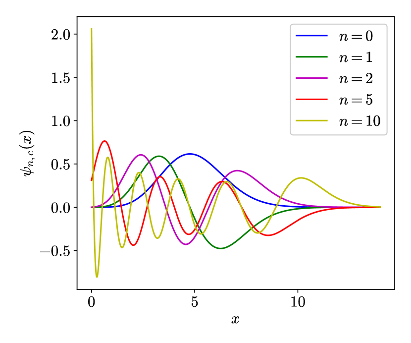
(a) $c=-10$

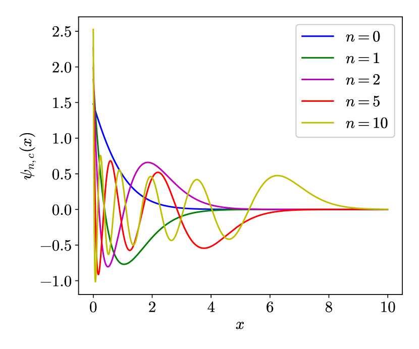
(b) $c=0$

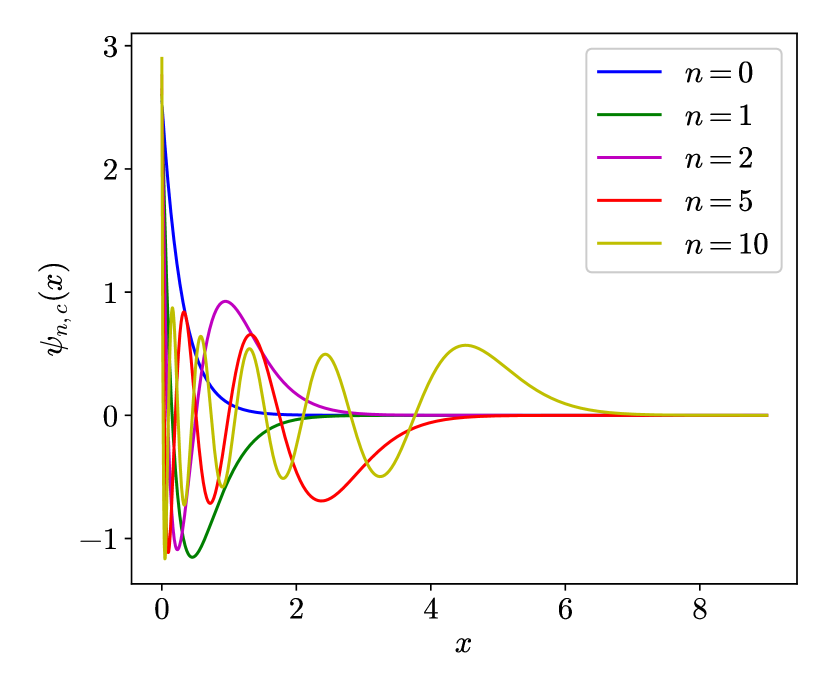
(c) $c=10$

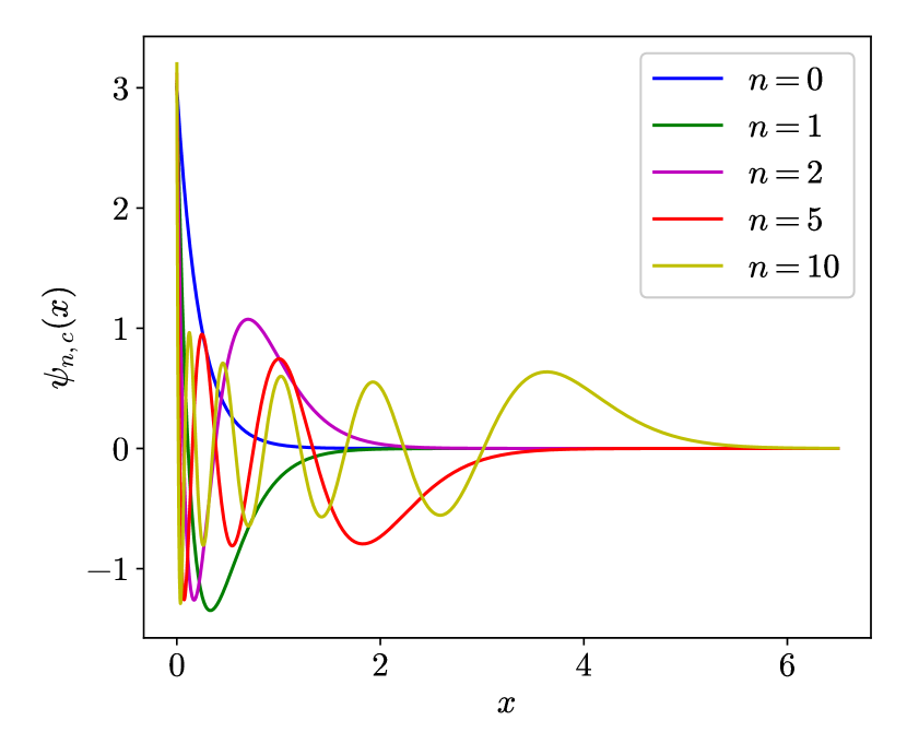
(d) $c=20$

Figure 1: Eigenfunctions $\psi_{n,c}$, defined by (8), of different orders with different parameters $c$.

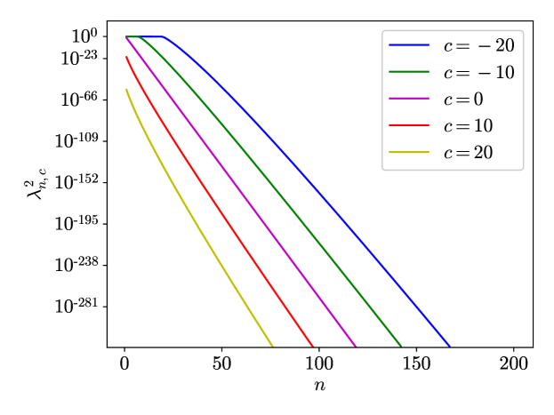
Figure 2: Squares of the spectra of the Airy integral operators $\mathcal{T}_{c}$ with different parameters $c$. This corresponds to the spectra of the integral operator $\mathcal{K}$ (see formulas (2), (117)). Note that the square of the leading eigenvalues converge to $1$ as $c\to-\infty$.

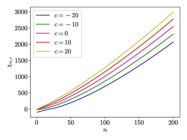
Figure 3: The spectra of the commuting differential operators $\mathcal{L}_{c}$ with different parameters $c$. Note the presence of negative eigenvalues for sufficiently negative values of $c$.

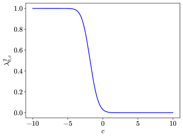
Figure 4: Squares of the first eigenvalues $\lambda_{0,c}$ of the Airy integral operators $\mathcal{T}_{c}$ with different parameters $c$. Note that $\lambda_{0,c}^{2}$ is equal to the maximal proportion of energy a function that is Airy-bandlimited to $[0,\infty)$ can have on $[c,\infty)$ (see Theorems 3.8 and 3.10).

$c$	$n$	$N$	Time
$20$	50	175	2.10$\times 10^{-3}$ secs
	100	230	3.64$\times 10^{-3}$ secs
	200	340	8.76$\times 10^{-3}$ secs
	400	560	3.35$\times 10^{-2}$ secs
$0$	50	155	3.36$\times 10^{-3}$ secs
	100	210	4.93$\times 10^{-3}$ secs
	200	320	9.75$\times 10^{-3}$ secs
	400	540	3.17$\times 10^{-2}$ secs
$-20$	50	175	4.32$\times 10^{-3}$ secs
	100	230	5.64$\times 10^{-3}$ secs
	200	340	1.14$\times 10^{-2}$ secs
	400	560	3.37$\times 10^{-2}$ secs

Table 1: The computation time of the eigenfunctions and spectra of the integral operator for different value of $c$ and $n$. The value of $N$ is determined by Observation 4.3. The time cost is of order $\mathcal{O}(N^{2})$.

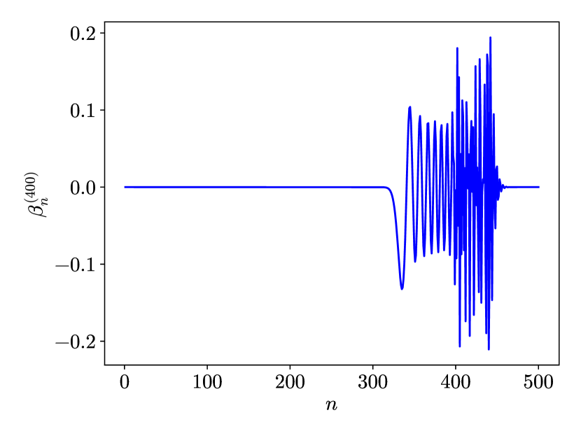
(a) $a=\widetilde{a}$

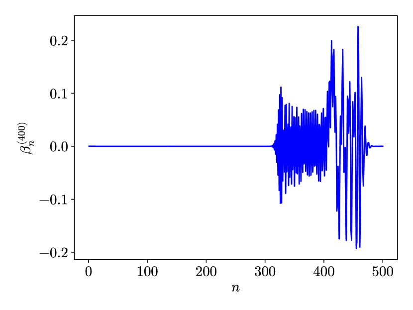
(b) $a=\widetilde{a}-4$

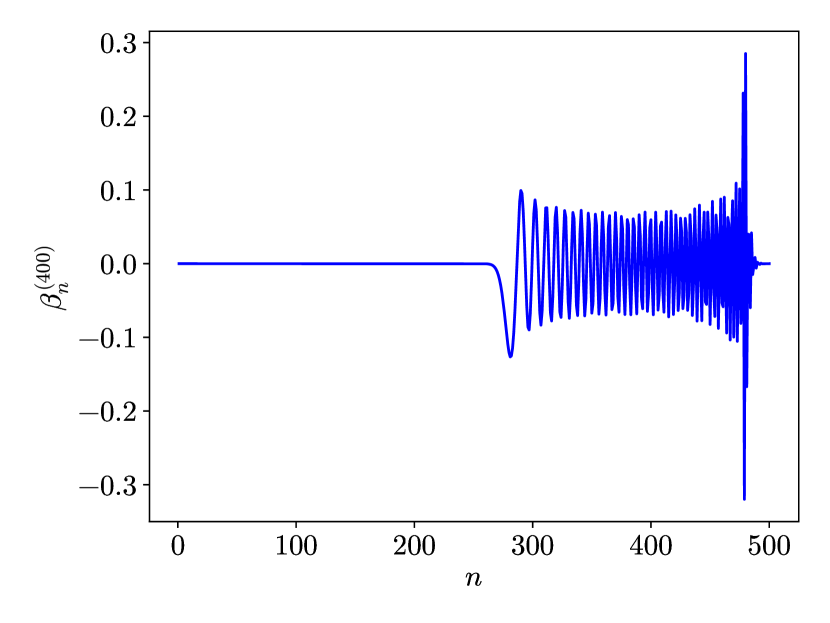
(c) $a=\widetilde{a}+4$

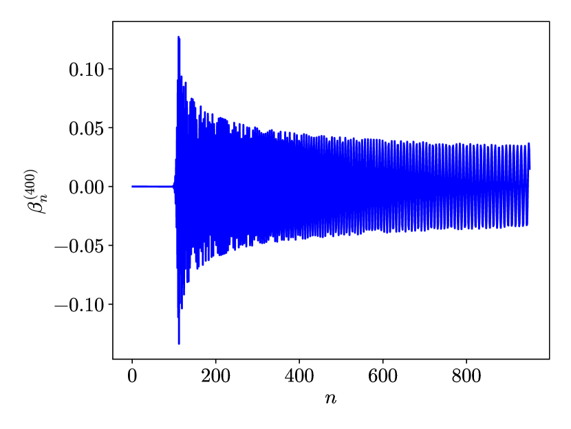
(d) $a=1$

Figure 5: Expansion coefficients of $\psi_{n,c}$ in the basis of scaled Laguerre functions with different scaling factors $a$, where $n=400$ and $c=10$. Note that the optimal scaling factor $\widetilde{a}\approx 20.62$, and is selected by formula (99). It’s clear that our basis functions become optimal when $a=\widetilde{a}$. Figure (5(d)) shows that the unscaled Laguerre functions are unsuitable for approximating the eigenfunctions of the Airy integral operator.

6.2 Computation of the distribution of the $k$-th largest eigenvalue of the Gaussian unitary ensemble

In this section, we report the computation time and the numerical errors of the PDF $\frac{d}{ds}F_{2}(k;s)$ and CDF $F_{2}(k;s)$ in Tables 2 and 3, for different values of $k$ and $s$. The reference solutions are computed by our solver using extended precision. We note that Prähofer tabulated the values of $F_{2}(1;s)$ and $\log\frac{d}{ds}F_{2}(1;s)$ to 16 digits of relative accuracy in [25], and our computed values match with the values reported there. We also show the plots of $\frac{d}{ds}F_{2}(k;s)$ and $F_{2}(k;s)$ for $k=1,2,3$ in Figure 6.

$k$	$s$	$n$	$N$	Time	Relative	Absolute	$\frac{d}{ds}F_{2}(k;s)$
					error	error
1	$50$	30	50	1.70$\times 10^{-4}$ secs	2.53$\times 10^{-14}$	3.76$\times 10^{-222}$	1.48437$\times 10^{-208}$
	$25$	20	40	1.20$\times 10^{-4}$ secs	1.16$\times 10^{-14}$	7.61$\times 10^{-90}$	6.56096$\times 10^{-76}$
	$10$	20	40	1.25$\times 10^{-4}$ secs	2.18$\times 10^{-15}$	4.14$\times 10^{-36}$	1.90064$\times 10^{-21}$
	$5$	20	40	1.36$\times 10^{-4}$ secs	3.28$\times 10^{-16}$	8.27$\times 10^{-25}$	2.52106$\times 10^{-9}$
	$2$	20	40	1.44$\times 10^{-4}$ secs	4.15$\times 10^{-15}$	1.57$\times 10^{-18}$	3.79199$\times 10^{-4}$
	$0$	20	40	1.50$\times 10^{-4}$ secs	2.07$\times 10^{-16}$	1.39$\times 10^{-17}$	6.69753$\times 10^{-2}$
	$-2$	20	40	1.49$\times 10^{-4}$ secs	5.03$\times 10^{-16}$	2.22$\times 10^{-16}$	4.41382$\times 10^{-1}$
	$-5$	40	60	2.96$\times 10^{-4}$ secs	7.25$\times 10^{-13}$	9.71$\times 10^{-17}$	1.34039$\times 10^{-4}$
	$-10$	50	80	4.39$\times 10^{-4}$ secs	2.53$\times 10^{-4}$	2.66$\times 10^{-39}$	1.05359$\times 10^{-35}$
	$-20$	70	120	9.45$\times 10^{-4}$ secs	8.50$\times 10^{87}$	1.50$\times 10^{-200}$	1.77193$\times 10^{-288}$
2	$30$	30	50	1.79$\times 10^{-4}$ secs	3.23$\times 10^{-14}$	2.85$\times 10^{-217}$	8.88120$\times 10^{-204}$
	$0$	20	40	1.50$\times 10^{-4}$ secs	1.11$\times 10^{-15}$	1.36$\times 10^{-20}$	1.21766$\times 10^{-5}$
	$-4$	30	50	2.23$\times 10^{-4}$ secs	3.08$\times 10^{-15}$	1.55$\times 10^{-15}$	5.05206$\times 10^{-1}$
	$-6$	50	80	4.88$\times 10^{-4}$ secs	1.43$\times 10^{-13}$	3.02$\times 10^{-16}$	2.10626$\times 10^{-3}$
	$-10$	50	100	7.38$\times 10^{-4}$ secs	1.35$\times 10^{-6}$	2.27$\times 10^{-30}$	1.67893$\times 10^{-24}$
	$-12$	60	120	1.07$\times 10^{-3}$ secs	2.80$\times 10^{-2}$	3.20$\times 10^{-48}$	1.14082$\times 10^{-46}$
3	$15$	30	50	2.46$\times 10^{-4}$ secs	4.10$\times 10^{-15}$	1.02$\times 10^{-140}$	2.48166$\times 10^{-126}$
	$4$	20	40	2.11$\times 10^{-4}$ secs	1.50$\times 10^{-15}$	8.21$\times 10^{-48}$	5.50657$\times 10^{-33}$
	$-4$	30	50	3.03$\times 10^{-4}$ secs	1.15$\times 10^{-14}$	1.44$\times 10^{-15}$	1.25051$\times 10^{-1}$
	$-8$	50	80	5.69$\times 10^{-4}$ secs	5.81$\times 10^{-12}$	1.03$\times 10^{-16}$	1.76988$\times 10^{-5}$
	$-10$	50	100	8.19$\times 10^{-4}$ secs	1.07$\times 10^{-8}$	8.56$\times 10^{-24}$	8.01983$\times 10^{-16}$
	$-13$	60	120	1.27$\times 10^{-3}$ secs	1.61$\times 10^{-2}$	1.55$\times 10^{-48}$	9.63884$\times 10^{-47}$

Table 2: The evaluation of the probability density functions. The actual values of $\frac{d}{ds}F_{2}(k;s)$ are reported to 6 significant digits. Note that the relative accuracy degenerates when one evaluates $\frac{d}{ds}F_{2}(k;s)$ in the left tails of the distributions (see Section 5.1).

$k$	$s$	$n$	$N$	Time	Relative	Absolute	$F_{2}(k;s)$
					error	error
$1$	$50$	30	50	1.70$\times 10^{-4}$ secs	$<$1.00$\times 10^{-16}$	$<$1.00$\times 10^{-16}$	1.00000$\times 10^{0}$
	$25$	20	40	1.20$\times 10^{-4}$ secs	$<$1.00$\times 10^{-16}$	$<$1.00$\times 10^{-16}$	1.00000$\times 10^{0}$
	$10$	20	40	1.25$\times 10^{-4}$ secs	$<$1.00$\times 10^{-16}$	$<$1.00$\times 10^{-16}$	1.00000$\times 10^{0}$
	$5$	20	40	1.36$\times 10^{-4}$ secs	$<$1.00$\times 10^{-16}$	$<$1.00$\times 10^{-16}$	1.00000$\times 10^{0}$
	$2$	20	40	1.44$\times 10^{-4}$ secs	1.11$\times 10^{-16}$	1.11$\times 10^{-16}$	9.99888$\times 10^{-1}$
	$0$	20	40	1.50$\times 10^{-4}$ secs	1.15$\times 10^{-16}$	1.11$\times 10^{-16}$	9.69373$\times 10^{-1}$
	$-2$	20	40	1.49$\times 10^{-4}$ secs	4.03$\times 10^{-16}$	1.67$\times 10^{-16}$	4.41322$\times 10^{-1}$
	$-5$	40	60	2.96$\times 10^{-4}$ secs	1.39$\times 10^{-12}$	2.96$\times 10^{-17}$	2.13600$\times 10^{-5}$
	$-10$	50	80	4.39$\times 10^{-4}$ secs	3.07$\times 10^{-4}$	1.29$\times 10^{-40}$	4.21226$\times 10^{-37}$
	$-20$	70	120	9.45$\times 10^{-4}$ secs	1.80$\times 10^{88}$	3.19$\times 10^{-202}$	1.77182$\times 10^{-290}$
2	$30$	30	50	1.79$\times 10^{-4}$ secs	$<$1.00$\times 10^{-16}$	$<$1.00$\times 10^{-16}$	1.00000$\times 10^{0}$
	$0$	20	40	1.50$\times 10^{-4}$ secs	1.11$\times 10^{-16}$	1.11$\times 10^{-16}$	9.99998$\times 10^{-1}$
	$-4$	30	50	2.23$\times 10^{-4}$ secs	1.04$\times 10^{-14}$	3.50$\times 10^{-15}$	3.35602$\times 10^{-1}$
	$-6$	50	80	4.88$\times 10^{-4}$ secs	2.99$\times 10^{-13}$	1.10$\times 10^{-16}$	3.69221$\times 10^{-4}$
	$-10$	50	100	7.38$\times 10^{-4}$ secs	1.70$\times 10^{-6}$	1.38$\times 10^{-31}$	8.14202$\times 10^{-26}$
	$-12$	60	120	1.07$\times 10^{-3}$ secs	3.30$\times 10^{-2}$	1.21$\times 10^{-49}$	3.65917$\times 10^{-48}$
3	$15$	30	50	2.46$\times 10^{-4}$secs	$<$1.00$\times 10^{-16}$	$<$1.00$\times 10^{-16}$	1.00000$\times 10^{0}$
	$4$	20	40	2.11$\times 10^{-4}$ secs	$<$1.00$\times 10^{-16}$	$<$1.00$\times 10^{-16}$	1.00000$\times 10^{0}$
	$-4$	30	50	3.03$\times 10^{-4}$ secs	$<$1.00$\times 10^{-16}$	$<$1.00$\times 10^{-16}$	9.59838$\times 10^{-1}$
	$-8$	50	80	5.69$\times 10^{-4}$ secs	9.70$\times 10^{-12}$	2.03$\times 10^{-17}$	2.09567$\times 10^{-6}$
	$-10$	50	100	8.19$\times 10^{-4}$ secs	1.42$\times 10^{-8}$	6.93$\times 10^{-25}$	4.89120$\times 10^{-17}$
	$-13$	60	120	1.27$\times 10^{-3}$ secs	1.89$\times 10^{-2}$	5.63$\times 10^{-50}$	2.98361$\times 10^{-48}$

Table 3: The evaluation of the cumulative distribution functions. The actual values of $F_{2}(k;s)$ are reported to 6 significant digits. Note that the relative accuracy degenerates when one evaluates $F_{2}(k;s)$ in the left tails of the distributions (see Section 5.1).

Observation 6.1.

The computation times of $\frac{d}{ds}F_{2}(k;s)$ and $F_{2}(k;s)$ are dominated by the calculation of the eigendecomposition of the Airy integral operator $\mathcal{T}_{s}$ (see Observation 5.2). As a consequence, the computation times of $\frac{d}{ds}F_{2}(k;s)$ and $F_{2}(k;s)$ are almost identical for any fixed $k$ and $s$ (see Tables 2, 3).

Observation 6.2.

Once the eigendecomposition of the Airy integral operator $\mathcal{T}_{s}$ is computed, the time cost of evaluating $F_{2}(k;s)$ and $\frac{d}{ds}F_{2}(k;s)$ via formulas (119) and (122) for different $k$ is relatively negligible (see Observation 5.2). We note that we only consider the evaluation of $\frac{d}{ds}F_{2}(k;s)$ and $F_{2}(k;s)$ for a single $k$ in our experiments, which means that the reported times include the time required for the computation of the eigendecomposition.

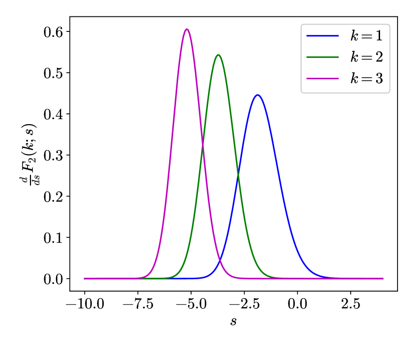
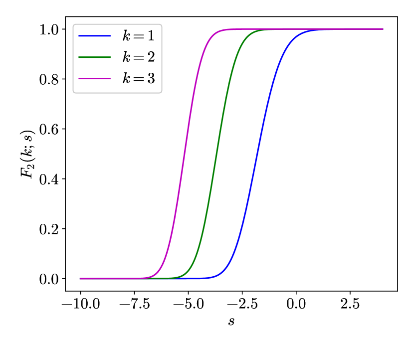
Figure 6: $\frac{d}{ds}F_{2}(k;s)$ and $F_{2}(k;s)$ for $k=1,2,3$.

Observation 6.3.

From Tables 2, 3 and Figure 6, it’s clear that our algorithm evaluates the distributions $\frac{d}{ds}F_{2}(k;s)$ and $F_{2}(k;s)$ to relative accuracy everywhere, except in the left tail. The algorithm only evaluates the left tail of the distributions to absolute precision, since the leading eigenvalues of the Airy integral operator $\mathcal{T}_{s}$ converge to $1$ as $s\to-\infty$ (see also Theorem 2.1), which leads to catastrophic cancellation in the computation of the distributions (see formulas (119), (122)).

6.3 Computation of finite-energy Airy beams

In this section, we compute the beam intensities for both the finite Airy beams and the Airy eigenfunction beams constructed from $\psi_{0,c}$, described in Section 5.2. In our experiments, we construct finite Airy beams and Airy eigenfunction beams with unit total energy, and with roughly the same intensity in their main lobes. We demonstrate that the eigenfunction beams are more non-diffracting than the finite Airy beams (see Figures 7, 8). We also plot the densities and beam intensities of the Airy eigenfunction beams at $\xi=0$ for various values of the parameter $c$ in Figure 9.

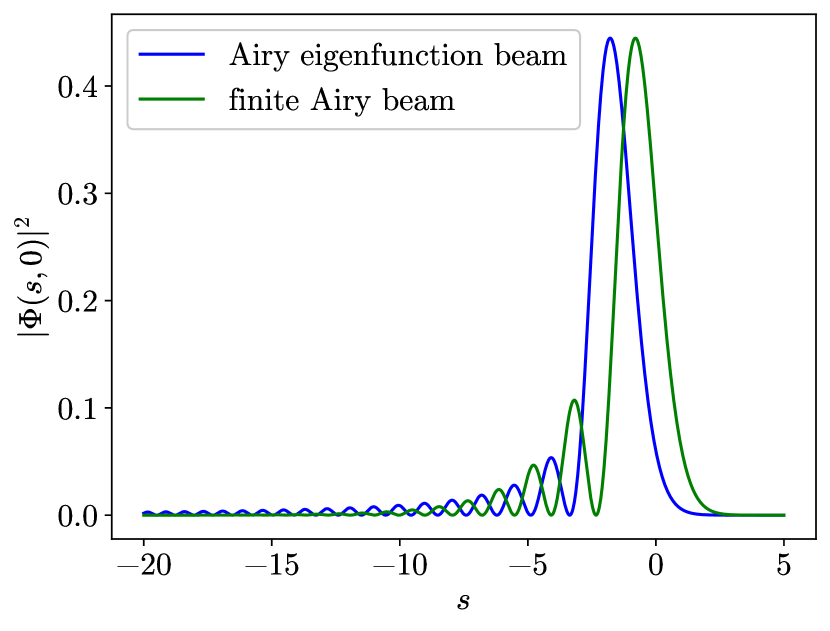
(a)

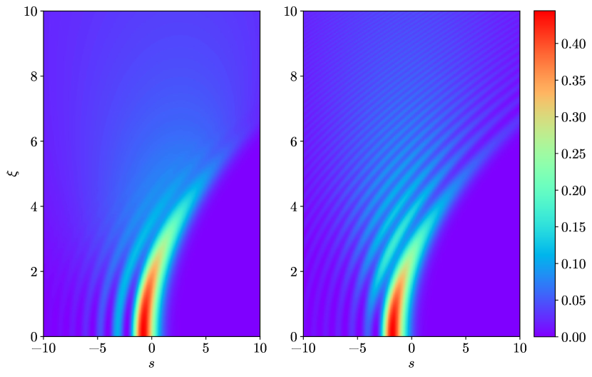
(b)

Figure 7: The intensity profiles of the finite Airy beam with parameter $\alpha=0.202$ and the Airy eigenfunction beam with parameter $c=-2$. The initial intensity profiles are shown in Figure (7(a)). The beam profiles of the finite Airy beam and the Airy eigenfunction beam are shown on the left and right of Figure (7(b)), respectively.

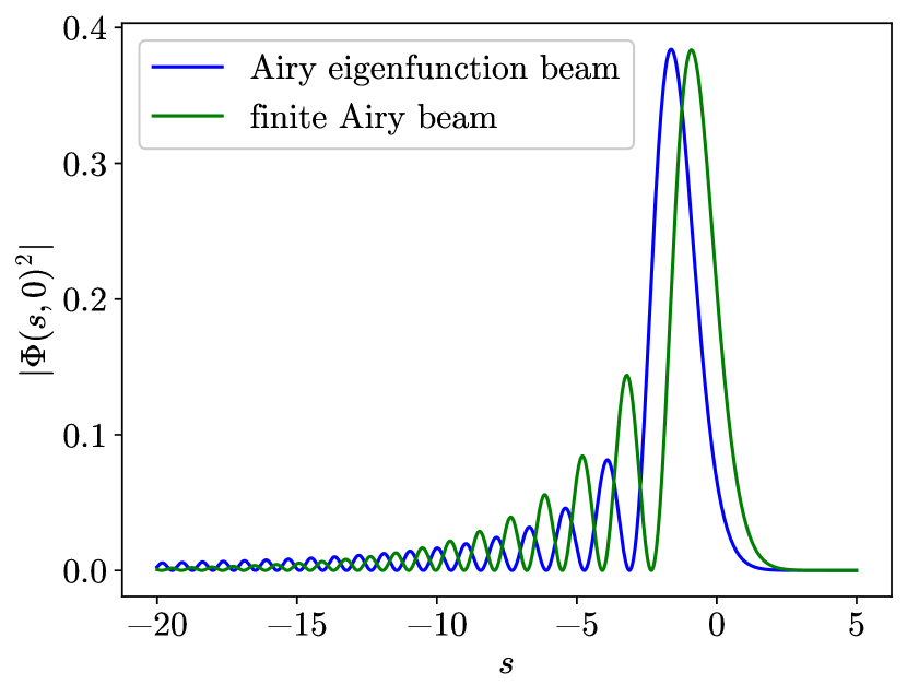
(a)

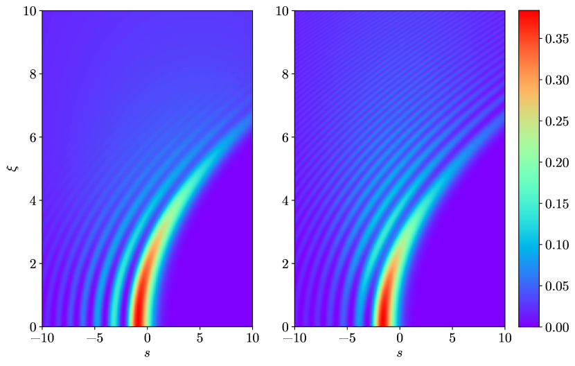
(b)

Figure 8: The intensity profiles of the finite Airy beam with parameter $\alpha=0.108$ and the optimal finite-energy Airy beam with parameter $c=-1$. The initial intensity profiles are shown in (8(a)). The beam profiles of the finite Airy beam and the Airy eigenfunction beam are shown on the left and right of Figure (8(b)), respectively.

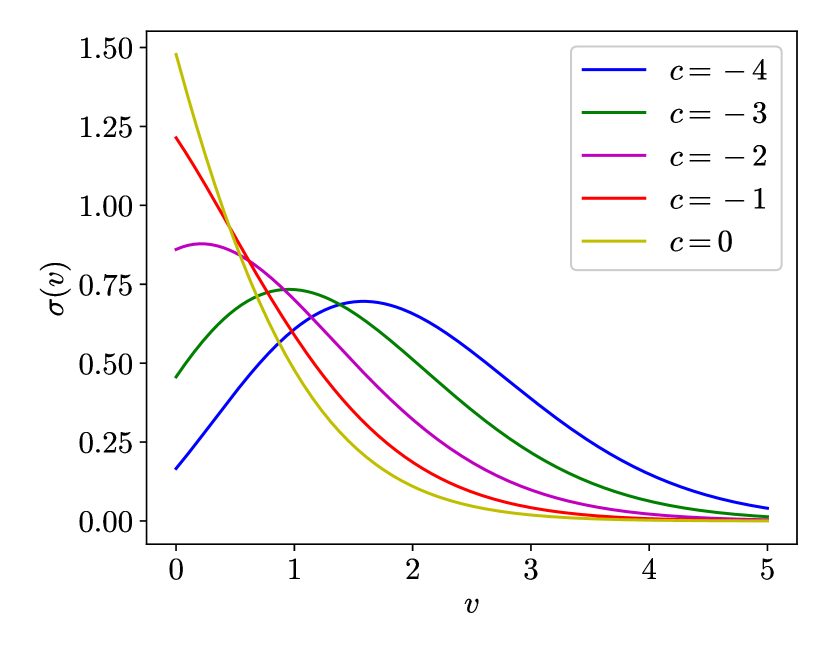
(a)

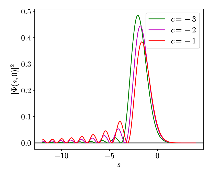
(b)

Figure 9: The density functions and beam intensities of the Airy eigenfunction beams, constructed from $\psi_{0,c}$, for various values of the parameter $c$. The density functions $\sigma(v)=\psi_{0,c}(v)$ and their corresponding beam intensities ${\lvert\Phi(s,0)\rvert}^{2}$, defined by formula (150), are shown in Figures (9(a)) and (9(b)), respectively, for various values of the parameter $c$.

Observation 6.4.

From Figures 7 and 8, it’s clear that the Airy eigenfunction beams exhibit the key characteristics of the Airy beam. Moreover, the Airy eigenfunction beams do a better job in preserving fine structure than the finite Airy beams, which implies that the Airy eigenfunction beams have both a better self-healing ability, and stronger gradient forces.

7 Conclusions

In this paper, we present a numerical algorithm for rapidly evaluating the eigendecomposition of the Airy integral operator $\mathcal{T}_{c}$, defined in (6). Our method computes the eigenvalues $\lambda_{j,c}$ of $\mathcal{T}_{c}$ to full relative accuracy, and computes the eigenfunctions $\psi_{j,c}$ of $\mathcal{T}_{c}$ and $\mathcal{L}_{c}$ in the form of an expansion (86) in scaled Laguerre functions, where the expansion coefficients are also computed to full relative accuracy. In addition, we characterize the previously unstudied eigenfunctions of the Airy integral operator, and describe their extremal properties in relation to an uncertainty principle involving the Airy transform.

We also describe two applications. First, we show that this algorithm can be used to rapidly evaluate the distributions of the $k$-th largest level at the soft edge scaling limit of Gaussian ensembles to full relative precision rapidly everywhere, except in the left tail (the left tail is computed to absolute precision). Second, we show that the eigenfunctions of the Airy integral operator can be used to construct finite-energy Airy beams that achieve the longest possible diffration-free distances by spreading their energy as evenly as possible in their side lobes, while also concentrating energy near the main lobes of their initial profiles.

8 Acknowledgements

We sincerely thank Jeremy Quastel for his helpful advice and for our informative conversations. The first author would like to thank Shen Zhenkun and Gu Qiaoling for their endless support, and he is fortunate, grateful, and proud of being their grandson.

Appendix A Appendix: Miscellaneous Properties of the Airy integral operator and its commuting differential operator

In this section, we describe miscellaneous properties of the eigenfunctions $\psi_{n,c}$ of the operators $\mathcal{T}_{c}$ and $\mathcal{L}_{c}$, as well as properties of the eigenvalues $\chi_{n,c}$ of the commuting differential operator $\mathcal{L}_{c}$, and $\lambda_{n,c}$ of the Airy integral operators $\mathcal{T}_{c}$.

A.1 Derivative of $\chi_{n,c}$ with respect to $c$

Theorem A.1.

For all real number $c$ and non-negative integers $n$,

$$\frac{\partial\chi_{n,c}}{\partial c}=\int_{0}^{\infty}x\bigl{(}\psi_{n,c}(x)\bigr{)}^{2}\,\mathrm{d}x.$$ (151)

Proof. By (20), we have

$$\frac{d}{dx}\Bigl{(}x\frac{d}{dx}\psi_{n,c}\Bigr{)}-(x^{2}+cx-\chi_{n})\psi_{n,c}=0.$$ (152)

With the infinitesimal change $c=c+h$, it follows that $\chi_{n}=\chi_{n}+\epsilon$, $\psi_{n,c}(x)=\psi_{n,c}(x)+\delta(x)$. Therefore, (152) becomes

$$\frac{d}{dx}\Bigl{(}x\frac{d}{dx}(\psi_{n,c}+\delta)\Bigr{)}-\bigl{(}x^{2}+(c+h)x-(\chi_{n}+\epsilon)\bigr{)}(\psi_{n,c}+\delta)=0.$$ (153)

After subtracting (152) from (153) and discarding infinitesimals of second order or greater, (153) becomes

$$\mathcal{L}_{c}[\delta](x)-(hx-\epsilon)\psi_{n,c}(x)=0,$$ (154)

where $\mathcal{L}_{c}$ is defined by (19). Then, we multiply both sides of (154) by $\frac{\psi_{n,c}(x)}{h}$ and integrate both sides over the interval $[0,\infty)$, which gives us

$$\frac{1}{h}\int_{0}^{\infty}\mathcal{L}_{c}[\delta](x)\psi_{n,c}(x)\,\mathrm{d}x-\int_{0}^{\infty}x\bigl{(}\psi_{n,c}(x)\bigr{)}^{2}\,\mathrm{d}x+\frac{\epsilon}{h}\int_{0}^{\infty}\bigl{(}\psi_{n,c}(x)\bigr{)}^{2}=0.$$ (155)

Due to the self-adjointness of $\mathcal{L}_{c}$,

$$\frac{1}{h}\int_{0}^{\infty}\mathcal{L}_{c}[\delta](x)\psi_{n,c}(x)\,\mathrm{d}x=\frac{1}{h}\int_{0}^{\infty}\delta(x)\mathcal{L}_{c}[\psi_{n,c}](x)\,\mathrm{d}x=0.$$ (156)

By (156) and the fact that ${\lVert\psi_{n,c}\rVert}_{2}=1$, in the appropriate limit, (155) becomes

$$\frac{\partial\chi_{n,c}}{\partial c}=\int_{0}^{\infty}x\bigl{(}\psi_{n,c}(x)\bigr{)}^{2}\,\mathrm{d}x.$$ (157)

$\blacksquare$

A.2 Recurrence relations involving the derivatives of eigenfunctions of different orders

Theorem A.2.

For all real numbers $c$, non-negative integers $n$, and $x\in[0,\infty)$,

$$-k(k-1)\psi_{n,c}^{(k-2)}(x)-k(c+2x)\psi_{n,c}^{(k-1)}(x)+\left(\chi_{n,c}-cx-x^{2}\right)\psi_{n,c}^{(k)}(x)$$

$$+(k+1)\psi_{n,c}^{(k+1)}(x)+x\psi_{n,c}^{(k+2)}(x)=0,$$ (158)

for all $k\geq 2$. Furthermore,

$$-(c+2x)\psi_{n,c}(x)+(\chi_{n,c}-cx-x^{2})\psi_{n,c}^{\prime}(x)+2\psi_{n,c}^{\prime\prime}(x)+x\psi_{n,c}^{(3)}(x)=0.$$ (159)

In particular, for all positive real $c$, non-negative integers $n$,

$$\chi_{n,c}\psi_{n,c}(0)+\psi_{n,c}^{\prime}(0)=0,$$ (160)

$$\psi_{n,c}(0)\neq 0.$$ (161)

Proof. The identities (A.2) and (159) are immediately obtained by repeated differentiation of (20). The identity (160) is proved by substituting $x=0$ into (20). Finally, the identity (161) can be easily verified via proof by contradiction. $\blacksquare$

Remark A.1.

We can compute the initial conditions $\psi_{n,c}(x)$ and $\psi_{n,c}^{\prime}(x)$ by evaluating the truncated expansion (96) and its first derivative in $\mathcal{O}(N)$ operations, where $N$ represents the number of the expansion coefficients. The higher derivatives can then be calculated via identities (20), (159) and (A.2) in $\mathcal{O}(1)$ operations. This theorem is useful for computing the Taylor expansion of $\psi_{n,c}$ at a given point $x$.

Corollary A.3.

For all positive real $c$, non-negative integers $m,n$,

$$(\chi_{m,c}-\chi_{n,c})\psi_{m,c}(0)\psi_{n,c}(0)+\psi_{m,c}^{\prime}(0)\psi_{n,c}(0)-\psi_{m,c}(0)\psi_{n,c}^{\prime}(0)=0.$$ (162)

Proof. The corollary follows directly from the identity (160). $\blacksquare$

A.3 Expansions in eigenfunctions

Given a real number $c$, the functions $\psi_{0,c},\psi_{1,c},\dots$ are a complete orthonormal basis in $L^{2}[0,\infty)$. Thus, every $f\in L^{2}[0,\infty)$ admits an expansion in the basis $\{\psi_{n,c}\}$. In this subsection, we’ll provide identities for the expansion coefficients of $\psi_{n,c}^{\prime},\psi_{n,c}^{\prime\prime},x\psi_{n,c}$ and $\frac{\partial\psi_{n}}{\partial c}$, in the basis $\{\psi_{n,c}\}$.

Theorem A.4.

For any real $c$, non-negative integers $m,n$,

$$\int_{0}^{\infty}\psi_{n}^{\prime}(x)\psi_{m}(x)\,\mathrm{d}x=-\frac{\lambda_{m}}{\lambda_{n}+\lambda_{m}}\psi_{n}(0)\psi_{m}(0),$$ (163)

and if $m\neq n$, then

$$\int_{0}^{\infty}\psi_{n}^{\prime\prime}(x)\psi_{m}(x)\,\mathrm{d}x=\frac{\lambda_{m}}{\lambda_{n}-\lambda_{m}}\Bigl{(}\psi_{n}^{\prime}(0)\psi_{m}(0)-\psi_{n}(0)\psi_{m}^{\prime}(0)\Bigr{)},$$ (164)

$$\int_{0}^{\infty}x\psi_{n}(x)\psi_{m}(x)\,\mathrm{d}x=\frac{\lambda_{n}\lambda_{m}}{\lambda_{n}^{2}-\lambda_{m}^{2}}\Bigl{(}\psi_{n}^{\prime}(0)\psi_{m}(0)-\psi_{n}(0)\psi_{m}^{\prime}(0)\Bigr{)},$$ (165)

$$\int_{0}^{\infty}\frac{\partial\psi_{n}}{\partial c}(x)\psi_{m}(x)\,\mathrm{d}x=\frac{\lambda_{n}\lambda_{m}}{\lambda_{m}^{2}-\lambda_{n}^{2}}\psi_{m}(0)\psi_{n}(0),$$ (166)

where $\psi_{m},\psi_{n},\lambda_{m},\lambda_{n}$ denote the eigenfunctions and eigenvalues of the Airy integral operator with parameter $c$.

Proof. To prove (163), we start with the identity

$$\lambda_{n}\int_{0}^{\infty}\psi_{n}^{\prime}(x)\psi_{m}(x)\,\mathrm{d}x=\int_{0}^{\infty}\Bigr{(}\int_{0}^{\infty}\frac{d}{dx}\text{Ai}(x+y+c)\psi_{n}(y)\,\mathrm{d}y\Bigl{)}\psi_{m}(x)\,\mathrm{d}x.$$ (167)

Note that

$$\frac{d}{dx}\text{Ai}(x+y+c)=\frac{d}{dy}\text{Ai}(x+y+c).$$ (168)

Therefore, the above calculation (167) can be repeated with $m$ and $n$ exchanged, yielding the identity

$$\lambda_{m}\int_{0}^{\infty}\psi_{m}^{\prime}(x)\psi_{n}(x)\,\mathrm{d}x= \int_{0}^{\infty}\Bigr{(}\int_{0}^{\infty}\frac{d}{dx}\text{Ai}(x+y+c)\psi_{m}(y)\,\mathrm{d}y\Bigl{)}\psi_{n}(x)\,\mathrm{d}x$$

$$= \int_{0}^{\infty}\Bigr{(}\int_{0}^{\infty}\frac{d}{dy}\text{Ai}(y+x+c)\psi_{n}(x)\,\mathrm{d}x\Bigl{)}\psi_{m}(y)\,\mathrm{d}y.$$ (169)

By combining (167) and (169), we get

$$\int_{0}^{\infty}\psi_{n}^{\prime}(x)\psi_{m}(x)\,\mathrm{d}x=\frac{\lambda_{m}}{\lambda_{n}}\int_{0}^{\infty}\psi_{m}^{\prime}(x)\psi_{n}(x)\,\mathrm{d}x.$$ (170)

On the other hand, integrating the right side of (170) by parts and rearranging the terms gives (163).

In the following, we assume that $m\neq n$.

To prove formula (164), we first combine (3), (8), and derive the following identity:

$$\lambda_{n}\psi_{n}^{\prime\prime}(x)=\int_{0}^{\infty}(x+y+c)\text{Ai}(x+y+c)\psi_{n}(y)\,\mathrm{d}y.$$ (171)

By repeating the same procedure (167)-(170), we get

$$\int_{0}^{\infty}\psi_{n}^{\prime\prime}(x)\psi_{m}(x)\,\mathrm{d}x=\frac{\lambda_{m}}{\lambda_{n}}\int_{0}^{\infty}\psi_{m}^{\prime\prime}(x)\psi_{n}(x)\,\mathrm{d}x.$$ (172)

Integrating the right side of (172) by parts twice and rearranging the terms gives (164).

To prove (165), first note that by combining (171) and (8), we get

$$\lambda_{n}\Bigl{(}\psi_{n}^{\prime\prime}(x)-(x+c)\psi_{n}(x)\Bigr{)}=\int_{0}^{\infty}y\text{Ai}(x+y+c)\psi_{n}(y)\,\mathrm{d}y.$$ (173)

Taking the inner product of both sides of (173) with $\psi_{m}(x)$, we have

$$\lambda_{n}\int_{0}^{\infty}\Bigl{(}\psi_{n}^{\prime\prime}(x)-(x+c)\psi_{n}(x)\Bigr{)}\psi_{m}(x)\,\mathrm{d}x= \int_{0}^{\infty}\int_{0}^{\infty}y\text{Ai}(x+y+c)\psi_{n}(y)\,\mathrm{d}y\,\psi_{m}(x)\,\mathrm{d}x$$

$$= \int_{0}^{\infty}y\psi_{n}(y)\int_{0}^{\infty}\text{Ai}(y+x+c)\psi_{m}(x)\,\mathrm{d}x\,\,\mathrm{d}y$$

$$= \,\lambda_{m}\int_{0}^{\infty}y\psi_{n}(y)\psi_{m}(y)\,\mathrm{d}y.$$ (174)

Therefore, (174) becomes

$$(\lambda_{m}+\lambda_{n})\int_{0}^{\infty}x\psi_{n}(x)\psi_{m}(x)\,\mathrm{d}x=\lambda_{n}\int_{0}^{\infty}\Bigl{(}\psi_{n}^{\prime\prime}(x)-c\psi_{n}(x)\Bigr{)}\psi_{m}(x)\,\mathrm{d}x.$$ (175)

By combining the orthogonality of $\psi_{n}$ and (164), we prove (165).

To prove (166), we take the derivative with respect to $c$ of both sides of (8), yielding the identity

$$\frac{\partial\lambda_{n}}{\partial c}\psi_{n}(x)+\lambda_{n}\frac{\partial\psi_{n}}{\partial c}(x)=\int_{0}^{\infty}\Bigl{(}\frac{d}{dc}\text{Ai}(x+y+c)\psi_{n}(y)+\text{Ai}(x+y+c)\frac{\partial\psi_{n}}{\partial c}(y)\Bigr{)}\,\mathrm{d}y.$$ (176)

Taking the inner product of both sides of (176) with $\psi_{m}(x)$, by (8), we get

$$\lambda_{n}\int_{0}^{\infty}\frac{\partial\psi_{n}}{\partial c}(x)\psi_{m}(x)\,\mathrm{d}x$$

$$=\int_{0}^{\infty}\Bigl{(}\int_{0}^{\infty}\frac{d}{dc}\text{Ai}(x+y+c)\psi_{n}(y)\,\mathrm{d}y\Bigr{)}\psi_{m}(x)\,\mathrm{d}x+\lambda_{m}\int_{0}^{\infty}\frac{\partial\psi_{n}}{\partial c}(y)\psi_{m}(y)\,\mathrm{d}y.$$ (177)

Since

$$\frac{d}{dx}\text{Ai}(x+y+c)=\frac{d}{dc}\text{Ai}(x+y+c),$$ (178)

we have that

$$\lambda_{n}\psi_{n}^{\prime}(x)=\int_{0}^{\infty}\frac{d}{dc}\text{Ai}(x+y+c)\psi_{n}(y)\,\mathrm{d}y.$$ (179)

Therefore,

$$\int_{0}^{\infty}\Bigl{(}\int_{0}^{\infty}\frac{d}{dc}\text{Ai}(x+y+c)\psi_{n}(y)\,\mathrm{d}y\Bigr{)}\psi_{m}(x)\,\mathrm{d}x=\lambda_{n}\int_{0}^{\infty}\psi_{n}^{\prime}(x)\psi_{m}(x)\,\mathrm{d}x.$$ (180)

Finally, by combining (163), (177) and (180), we prove (166). $\blacksquare$

A.4 Behavior of the eigenfunction $\psi_{n,c}$ as $c\to\infty$

In this section, we show that the eigenfunction $\psi_{n,c}$ of the Airy integral operator $\mathcal{T}_{c}$ converges to a scaled Laguerre function in the limit as $c\to\infty$.

Theorem A.5.

As $c\to\infty$,

$$\psi_{n,c}(x)\to h_{n}^{2\sqrt{c}}(x),$$ (181)

where $h_{n}^{2\sqrt{c}}$ is the scaled Laguerre function defined in (26) with parameter $a=2\sqrt{c}$.

Proof. As $c\to\infty$, $\psi_{n,c}$ converges to the solution of

$$\frac{d}{dx}(x\frac{d}{dx}f)-cxf=-\chi_{n,c}f,$$ (182)

by formula (20) and the fact that $\psi_{n,c}$ becomes almost compactly supported in the limit as $c\to\infty$ (see Theorem 3.11). By comparing (182) and (33), we conclude that

$$\lim_{c\to\infty}\psi_{n,c}(x)=h_{n}^{2\sqrt{c}}(x).$$ (183)

$\blacksquare$

Corollary A.6.

$\lim_{c\to\infty}\chi_{n,c}=(2n+1)\sqrt{c}.$

Proof. This corollary is an immediate consequence of formulas (182) and (33). $\blacksquare$

A.5 Behavior of the eigenfunction $\psi_{n,c}$ as $c\to-\infty$

In this section, we show that the eigenfunction $\psi_{n,c}$ of the Airy integral operator $\mathcal{T}_{c}$ converges to a scaled and shifted Hermite function in the limit as $c\to-\infty$. We first introduce the mathematical preliminaries.

The Hermite polynomials, denoted by $H_{n}\colon\mathbbm{R}\to\mathbbm{R}$, are defined by the following three-term recurrence relation for any $k\geq 1$ (see [1]):

$$H_{n+1}(x)=2xH_{n}(x)-2nH_{n-1}(x),$$ (184)

with the initial conditions

$$H_{0}(x)=1,\quad H_{1}(x)=1-x.$$ (185)

The polynomials defined by the formulas (184) and (185) are an orthogonal basis in the Hilbert space induced by the inner product ${\langle f,g\rangle}=\int_{0}^{\infty}e^{-x^{2}}f(x)g(x)\,\mathrm{d}x$, i.e.,

$${\langle H_{n},H_{m}\rangle}=\int_{0}^{\infty}e^{-x^{2}}H_{n}(x)H_{m}(x)\,\mathrm{d}x=\sqrt{\pi}2^{n}n!\delta_{n,m}.$$ (186)

In addition, Hermite polynomials are solutions of Hermite’s equation:

$$f^{\prime\prime}-2xf^{\prime}+2nf=0.$$ (187)

We find it useful to use the scaled Hermite functions defined below.

Definition A.1.

Given a positive real number $a$, the scaled Hermite functions, denoted by $\phi_{n}^{a}\colon\mathbbm{R}\to\mathbbm{R}$, are defined by

$$\phi_{n}^{a}(x)=\frac{\sqrt{a}}{\pi^{\frac{1}{4}}2^{\frac{n}{2}}(n!)^{\frac{1}{2}}}e^{-a^{2}x^{2}/2}H_{n}(ax).$$ (188)

The scaled Hermite functions satisfy the differential equation

$$-\frac{d^{2}}{dx^{2}}\phi_{n}^{a}+a^{4}x^{2}\phi_{n}^{a}=a^{2}(2n+1)\phi_{n}^{a}.$$ (189)

Lemma A.7.

Given a negative real number $c$, define $g_{n}(u)=\psi_{n,c}((-\frac{c}{2})^{\frac{1}{4}}u-\frac{c}{2})$, where $\psi_{n,c}$ is the $(n+1)$-th eigenfunction of the Airy integral operator $\mathcal{T}_{c}$. Then, $g_{n}$ is the solution of the ODE

$$-\frac{d^{2}}{du^{2}}f-\bigl{(}-\frac{c}{2}\bigr{)}^{-\frac{3}{4}}\Bigl{(}u\frac{d^{2}}{du^{2}}f+\frac{d}{du}f\Bigr{)}+u^{2}f=\bigl{(}\bigl{(}-\frac{c}{2}\bigr{)}^{\frac{3}{2}}+\bigl{(}-\frac{c}{2}\bigr{)}^{-\frac{1}{2}}\chi_{n,c}\bigr{)}f,$$ (190)

where $\chi_{n,c}$ is the $(n+1)$-th eigenvalue of the commuting differential operator $\mathcal{L}_{c}$.

Proof. The lemma directly follows from the definition of $g_{n}$ and the differential equation satisfied by $\psi_{n,c}$ (see formula (20)). $\blacksquare$

Theorem A.8.

As $c\to-\infty$,

$$\psi_{n,c}(x)\to\frac{1}{\sqrt{a}}\phi_{n}^{a}\bigl{(}x+\frac{c}{2}\bigr{)},$$ (191)

where $a=(-\frac{c}{2})^{-\frac{1}{4}}$. In other words, $\psi_{n,c}(x)$ converges a Hermite function that is translated by $-\frac{c}{2}$, and scaled by scaling parameter $(-\frac{c}{2})^{-\frac{1}{4}}$.

Proof. As $c\to-\infty$, $g_{n}$ converges to the solution of

$$-\frac{d^{2}}{du^{2}}f+u^{2}f=\bigl{(}\bigl{(}-\frac{c}{2}\bigr{)}^{\frac{3}{2}}+\bigl{(}-\frac{c}{2}\bigr{)}^{-\frac{1}{2}}\chi_{n,c}\bigr{)}f,$$ (192)

since $\lim_{c\to-\infty}(-\frac{c}{2})^{-\frac{3}{4}}=0$. By comparing (192) and $(\ref{shode})$, we conclude that

$$\lim_{c\to-\infty}g_{n}(u)=\phi_{n}^{1}(u).$$ (193)

Therefore, by definition,

$$\lim_{c\to-\infty}\psi_{n,c}(x)=\phi_{n}^{1}\bigl{(}\bigl{(}-\frac{c}{2}\bigr{)}^{-\frac{1}{4}}\bigl{(}x+\frac{c}{2}\bigr{)}\bigr{)}=\frac{1}{\sqrt{a}}\phi_{n}^{a}\bigl{(}x+\frac{c}{2}\bigr{)},$$ (194)

where $a=(-\frac{c}{2})^{-\frac{1}{4}}$. $\blacksquare$

Corollary A.9.

$\lim_{c\to-\infty}\chi_{n,c}=(2n+1)(-\frac{c}{2})^{\frac{1}{2}}-\frac{c^{2}}{4}.$

Proof. This corollary is an immediate consequence of formulas (192) and (189). $\blacksquare$

References

- [1] Abramowitz, M., and I. A. Stegun. Handbook of Mathematical Functions With Formulas, Graphs, and Mathematical Tables. Washington: U.S. Govt. Print. Off., 1964.
- [2] Born, M. and E. Wolf. Principles of Optics. 6th ed. (with corrections). Pergamon Press, 1986.
- [3] Bornemann, F. “On the Numerical Evaluation of Distributions in Random Matrix Theory: A Review.” Markov Processes Relat. Fields 16.4 (2010): 803–866.
- [4] Bornemann, F. “On the numerical evaluation of Fredholm determinants.” Math. Comput. 79.270 (2010): 871–915.
- [5] Bouchaud, J. P., M. Potters. “Financial Applications of Random Matrix Theory: a short review.” Handbook on Random Matrix Theory. Oxford University Press, 2009.
- [6] Caspera, W. R., F. A. Grünbaum, M. Yakimova, and I. Zurriánc. “Reflective prolate-spheroidal operators and the KP/KdV equations.” PNAS 116.37 (2019): 18310–18315.
- [7] Chiani M. “Distribution of the largest eigenvalue for real Wishart and Gaussian random matrices and a simple approximation for the Tracy–Widom distribution.” J. Multivar. Anal. 129 (2014): 69–81.
- [8] Couillet, R. and M. Debbah. Random Matrix Methods for Wireless Communications. Cambridge University Press, 2011.
- [9] Deift, P. “Some Open Problems in Random Matrix Theory and the Theory of Integrable Systems. II.” SIGMA Symmetry Integrability Geom. Methods Appl. 13 (2017): 016
- [10] Dieng, M. “Distribution Functions for Edge Eigenvalues in Orthogonal and Symplectic Ensembles: Painlevé Representations.” PhD thesis, University of Davis. e-print: arXiv:math/0506586v2, 2005.
- [11] Edelman, A. and N.R. Rao. “Random matrix theory.” Acta Numer. 14 (2005): 233–297.
- [12] Edelman, A. and P.O. Persson. “Numerical methods for eigenvalue distributions of random matrices.” arXiv:math-ph/0501068, 2005.
- [13] Forrester, P.J. “The spectrum edge of random matrix ensembles.” Nuclear Phys. B 402.3 (1993): 709–728.
- [14] Guhr, T., A. Müller–Groeling, and H. A. Weidenüller. “Random-matrix theories in quantum physics: common concepts.” Phys. Rep. 299.4-6 (1998): 189–425.
- [15] Jiang, Y., K. Huang, X. Lu. “The optical Airy transform and its application in generating and controlling the Airy beam.” Opt. Commun. 285 (2012): 4840–4843.
- [16] Karoui, A., I. Mehrzi, and T. Moumni. “Eigenfunctions of the Airy’s integral transform: Properties, numerical computations and asymptotic behaviors.” J. Math. Anal. Appl. 389.2 (2012): 989–1005.
- [17] Lederman, R.R. “On the Analytical and Numerical Properties of the Truncated Laplace Transform.” Technical Report, YALEU/DCS/TR-1490 (2014)
- [18] Lederman, R.R, V. Rokhlin. “On the Analytical and Numerical Properties of the Truncated Laplace Transform I.” SIAM J. Numer. Anal. 53.3 (2014): 1214–1235.
- [19] Livan G., M. Novaes, P. Vivo. Introduction to Random Matrices: Theory and Practice. Springer 2018.
- [20] Levy, U., S. Derevyanko, and Y. Silberberg. “Light modes of free space.” Prog. Optics 61 (2016): 237–281.
- [21] Mehta, M. L. Random matrices. 3rd ed, Elsevier 2004.
- [22] Osipov, A. “Evaluation of small elements of the eigenvectors of certain symmetric tridiagonal matrices with high relative accuracy.” Appl. Comput. Harmon. Anal. 43.2 (2017): 173–211.
- [23] Osipov, A., V. Rokhlin, and H. Xiao. Prolate Spheroidal Wave Functions of Order Zero - Mathematical Tools for Bandlimited Approximation. Springer, 2013.
- [24] Paul, D. and A. Aue. “Random matrix theory in statistics: A review.” J. Stat. Plan. Inference 150 (2014): 1–29.
- [25] Prähofer, M. “Tables to: Exact scaling functions for one-dimensional stationary KPZ growth.” http://www-m5.ma.tum.de/KPZ/, 2003.
- [26] Schwarz, H. R. “Tridiagonalization of a symmetric band matrix.” Numer. Math. 12.4 (1968): 231–241.
- [27] Siviloglou, G.A. and D.N. Christodoulides. “Accelerating finite energy Airy beams.” Opt. Lett. 32.8 (2007): 979–981.
- [28] Siviloglou, G.A., J. Broky, A. Dogarium and D.N. Christodoulides. “Observation of accelerating Airy beams.” Phys. Rev. Lett. 99.213901 (2007).
- [29] Slepian, D. and H. O. Pollak. “Prolate Spheroidal Wave Functions, Fourier Analysis and Uncertainty—I”, Bell Syst. Tech. J. 40.1 (1961): 43–63.
- [30] Tracy, C. A. and H. Widom. “Level-Spacing Distributions and the Airy Kernel.” Commun. Math. Phys. 159 (1994): 151–174.
- [31] Trefethen, L.N. and D. Bau. Numerical Linear Algebra. SIAM, 1997.
- [32] Turunen, J., and A. T. Friberg. “Propagation-invariant optical fields.” Prog. Optics 54 (2010): 1–88.
- [33] Valleé, O. and M. Soares. Airy Functions and Applications to Physics. Imperial College Press, 2004.
- [34] Xiang, S. “Asymptotics on Laguerre or Hermite polynomial expansions and their applications in Gauss quadrature.” J. Math. Anal. Appl. 393.2 (2012): 434–444.