Unitarisation dependence of diffractive scattering in light of high-energy collider data

Abstract

We study the consequences of high-energy collider data on the best fits to total, elastic, inelastic, and single-diffractive cross sections for $pp$ and $p\bar{p}$ scattering using different unitarisation schemes. We find that the data are well fitted both by eikonal and U-matrix schemes, but that diffractive data prefer the U-matrix. Both schemes may be generalised by means of an additional parameter; however, this yields only marginal improvements to the fits. We provide estimates for $\rho$, the ratio of the real part to the imaginary part of the elastic amplitude, for the different fits. We comment on the effect of the different schemes on present and future cosmic ray data.

1 Introduction

High-energy hadronic scattering may be described by Reggeon exchanges (see, e.g. Donnachie:2013xia and references therein) and for center-of-momentum energies $\sqrt{s}$ larger than 100 GeV, the only trajectory that matters is that of the pomeron. However, at energies of a few TeV and higher, the growth of the pomeron term leads to violation of the black-disk limit Gotsman:1993ux ; Shoshi:2002in ; Selyugin:2004sy and eventually of unitarity. Unitarity can be enforced in high-energy $pp$ and $p\bar{p}$ interactions by the inclusion of multiple exchanges, which act as a cut to the elastic scattering amplitude. Different unitarisation schemes have been discussed in the literature Cudell:2008yb but all of them rely on phenomenological arguments in the absence of a comprehensive quantum chromodynamics treatment.

The effect of unitarisation on the growth of $p\overset{\scriptscriptstyle\left(-\right)}{p}$ cross-sections becomes important when considering proton-proton scattering cross sections at the LHC where the centre-of-momentum energies extend up to 13 TeV. Measurements of the total, elastic, inelastic, and diffractive $pp$ cross sections by the different LHC experiments — ALICE Abelev:2012sea , ATLAS Aad:2014dca ; Aaboud:2016ijx ; Aad:2011eu ; Myska:2017iqc , CMS Sirunyan:2018nqx , LHCb Aaij:2018okq , and TOTEM Antchev:2011vs ; Antchev:2013gaa ; Antchev:2013iaa ; Antchev:2013paa ; Antchev:2017dia ; Antchev:2013haa — add to existing $p\overset{\scriptscriptstyle\left(-\right)}{p}$ scattering data at lower energies from previous generation experiments at the S$p\bar{p}$S Bozzo:1984rk ; Alner:1986iy and the TeVatron Abe:1993xx ; Amos:1990jh ; Amos:1992zn ; Abe:1993wu ; Avila:1998ej ; Avila:2002bp . This extensive wealth of data allows us to constrain the nature of unitarisation governing these interactions with an improved degree of accuracy.

Differences in cross sections that depend on the choice of the unitarisation scheme are expected to show up at very high energies — at 10 TeV and higher — and therefore may influence predictions for cosmic-ray collisions with atmospheric nuclei at ultra-high energies. Showering codes, such as SIBYLL Engel:2019dsg and QGSJET Ostapchenko:2019few , used to simulate and reconstruct these events from observations of secondaries have historically used the eikonal scheme (see Anchordoqui:2004xb for a review). In the context of ongoing ultra-high energy cosmic-ray experiments, e.g. the Pierre Auger Observatory ThePierreAuger:2015rma , the Telescope Array Project Kawai:2008zza , and IceTop IceCube:2012nn , an investigation of the dependence of cross sections on different unitarisation schemes assumes paramount importance.

In Bhattacharya:2020lac , we examined the effect of including up-to-date collider data for total, elastic, and inelastic cross sections. We found nearly identical cross sections for the three irrespective of the unitarisation scheme used. In the current work, we focus on the effect of incorporating diffractive data into the fits. Diffractive scattering in $2\mapsto 2$ interactions, where either one or both final state particles break up into jets, becomes increasingly important as the interaction energy increases. In these interactions, the final state(s) being no longer expressible in terms of hadronic eigenstates, the calculation of the corresponding scattering amplitudes requires the invocation of a rotated eigenstate basis as described in the Good-Walker mechanism Good:1960ba .

The present work is organised as follows. In Section 2, we briefly recapitulate the theory of unitarisation in $p\overset{\scriptscriptstyle\left(-\right)}{p}$ scattering and the different schemes that have been proposed in the literature. In Section 3 we explain the Good-Walker representation Good:1960ba . In section 4 we list the various parameters defining our fits. Additionally, we list all the $p\overset{\scriptscriptstyle\left(-\right)}{p}$ scattering data that are used to determine our best fits. Finally, in Section 5 we give our results and discuss them in light of the existing literature, drawing our conclusions.

2 Brief survey of unitarisation schemes and fit to non-diffractive forward data

The differential cross section for elastic scattering may be expressed in terms of the elastic amplitude $A(s,t)$ as

$$\frac{\mathrm{d}\sigma_{el}}{\mathrm{d}t}=\frac{\big{\lvert}A(s,t)\big{\rvert}^{2}}{16\pi s^{2}}\,,$$ (1)

where $t=-\bm{q}^{2}$ is the square of the momentum transfer. At low energy, the term in $A(s,t)$ responsible for the growth of the cross section with $s$ can be parameterised Cudell:2005sg using the pomeron trajectory $\alpha(t)$, the proton elastic form factor $\mathcal{F}_{pp}(t)$ and the coupling pomeron-proton-proton $g_{pp}$, as

$$a(s,t)=g_{pp}^{2}\,\mathcal{F}_{pp}(t)^{2}\left(\frac{s}{s_{0}}\right)^{\alpha(t)}\,\xi(t),$$ (2)

with $\xi(t)$ the signature factor

$$\xi(t)=-e^{-i\pi\alpha(t)\over 2}.$$ (3)

We shall consider here a dipole form factor, which is close to the best functional form (Cudell:2005sg, ), although the exact functional form is not very important as we consider only integrated quantities in this paper:

$$\mathcal{F}_{pp}={1\over(1-t/t_{pp})^{2}}$$ (4)

The pomeron trajectory is close to a straight line Cudell:2003dz , and we take it to be

$$\alpha(t)=1+\epsilon+\alpha^{\prime}_{P}t.$$ (5)

At high energy, the growth of this pomeron term and eventual violation of unitarity is most clearly seen in the impact-parameter representation, where the Fourier transform of the amplitude $a\left(s,t\right)$ rescaled by $2s$ is equivalent to a partial wave

$$\chi(s,\bm{b})=\int\frac{\mathrm{d}^{2}\bm{q}}{\left(2\pi\right)^{2}}\frac{a(s,t)}{2s}\mathrm{e}^{\mathrm{i}\bm{q}\cdot\bm{b}}.$$ (6)

The norm of this partial wave at small $\big{\lvert}\bm{b}\big{\rvert}$ exceeds unity around $\sqrt{s}=2$ TeV Cudell:2003dz .

To solve this problem, one introduces unitarisation schemes which map the amplitude $\chi(s,\bm{b})$ to the physical amplitude $X(s,\bm{b})$. The latter reduces to $\chi(s,\bm{b})$ for small $s$, is confined to the unitarity circle $\big{\lvert}X(s,\bm{b})-i\big{\rvert}\leqslant 1$, and bears the same relation as Eq.(6), but this time to the physical amplitude:

$$X(s,\bm{b})=\int\frac{\mathrm{d}^{2}\bm{q}}{\left(2\pi\right)^{2}}\frac{A(s,t)}{2s}\mathrm{e}^{\mathrm{i}\bm{q}\cdot\bm{b}}.$$ (7)

The most common scheme is the eikonal scheme, and it has been derived for structureless bodies, in optics, in potential scattering and in QED. Another proposed scheme is the U matrix scheme, which can be motivated by a form of Bethe-Salpeter equation Logunov:1971jy . Probably neither of these is correct in QCD, but going from one to the other permits an evaluation of the systematics linked to unitarisation.

In the following, we shall actually use generalised versions of the schemes, which include an extra parameter $\omega$ Cudell:2008yb :

$$X_{E}(s,\bm{b})=\frac{\mathrm{i}}{\omega}\left[1-\mathrm{e}^{\mathrm{i}\omega\chi(s,\bm{b})}\right]\,,$$ (8)

while the generalised U-matrix scheme requires:

$$X_{U}(s,\bm{b})=\frac{\chi(s,\bm{b})}{1-\mathrm{i}\omega\chi(s,\bm{b})}.$$ (9)

In both cases, the asymptotic value of $X(s\to\infty,\bm{b})$ is $1/\omega$, hence the traditional values for $\omega$ are 1 for the standard eikonal Logunov:1971jy , and $1/2$ for the standard U matrix Savrin:1976zn . Both schemes map the amplitude $\chi(s,\bm{b})$ into the unitarity circle for $\omega\geqslant 1/2$. In terms of partial waves, the maximum inelasticity is reached for $X(s,\bm{b})=\mathrm{i}$.

The total and elastic scattering cross sections may be readily expressed in these representations as

$$\sigma_{{tot}} =2\int\!\mathrm{d}^{2}\bm{b}\ \mathfrak{Im}\left(X(s,\bm{b})\right), \sigma_{{el}} =\int\!\mathrm{d}^{2}\bm{b}\ \big{\lvert}X(s,\bm{b})\big{\rvert}^{2}.$$ (10)

Hence these unitarised schemes naturally lead to expressions for the total, elastic, and hence inelastic, cross sections. We shall now use them to fit all the data in $p\overset{\scriptscriptstyle\left(-\right)}{p}$ scattering above 100 GeV, for which lower trajectories have a negligible effect. This includes the following:

• $pp$ total and elastic cross sections from TOTEM Antchev:2011vs ; Antchev:2013gaa ; Antchev:2013iaa ; Antchev:2013paa ; Antchev:2017dia , and ATLAS Aad:2014dca ; Aaboud:2016ijx ;

• $p\bar{p}$ total and elastic cross sections from CDF Abe:1993xx , E710 Amos:1990jh ; Amos:1992zn , and E811 Avila:1998ej ; Avila:2002bp experiments at TeVatron; and UA4 at S$\rm p\bar{p}$S Bozzo:1984rk ;

• Direct measurements of inelastic cross sections, i.e. not derived from total and elastic measurements, from UA5 at S$\rm p\bar{p}$S Alner:1986iy , ATLAS Aad:2011eu ; Myska:2017iqc , LHCb Aaij:2018okq , ALICE Abelev:2012sea , and TOTEM Antchev:2013haa .

This gives a total of 37 data points. In the next section, we shall also consider 6 extra data points:

• Single diffractive $p\bar{p}$ cross sections from UA5 Alner:1986iy ; Alner:1987wb and E710 Amos:1992jw ; and

• $pp$ single diffractive cross sections at various energies measured at ALICE Abelev:2012sea .

The resulting fit leads to the following parameters of Table 1.

Scheme	$\epsilon$	$\alpha^{\prime}_{P}$ (GeV-2)	$g_{pp}$	$t_{pp}$ (GeV2)	$\chi^{2}/\text{d.o.f}$
U-matrix	$0.10\pm 0.01$	$0.37\pm 0.28$	$7.5\pm 0.8$	$2.5\pm 0.6$	$1.436$
Eikonal	$0.11\pm 0.01$	$0.31\pm 0.19$	$7.3\pm 0.9$	$1.9\pm 0.4$	$1.442$

Table 1: $\chi^{2}$/d.o.f and best-fit parameters obtained using the eikonal ($\omega=1$) and U-matrix ($\omega^{\prime}=1/2$) unitarisation schemes without diffractive data Bhattacharya:2020lac .

3 Unitarisation and diffraction

The implementation of diffraction within a unitarisation scheme at high energy has to confront two questions: how does one describe the diffractive amplitude at the Born level, and how does one embed that amplitude within a unitarisation scheme?

The first questions has two answers. On the one hand, the asymptotic answer is that , for high-mass final states, one should use the triple-reggeon vertices. However, as the masses considered are not necessarily large, one must consider a variety of reggeons lying on trajectories below that of the pomeronDonnachie:2003ec , and to include not only subdominant trajectories (with intercept of the order of $1/2$) but also sub-subdominant ones (with an intercept of the order of 0). This introduces a multitude of parameters, of the order of the number of high-energy data points available.

On the other hand, it is possible to consider a generic diffractive state $D$ and the vertex $p+I\!\!P\to D$. A priori, this implies the consideration of a large number of channels for the diffractive state $D$, and the introduction of many parameters. However, it has been shown in Gotsman:1999xq that for inclusive cross section, the consideration of one generic diffractive state $\mid\Psi_{D}\rangle$ is sufficient, and that adding other states does not significantly improve the description of the data. One however looses the information about the mass of the diffractive state.

We will concentrate in this paper on inclusive quantities, and on a generic diffractive $D$, which is the seed of high-energy pions, and hence of high-energy muons, in cosmic ray showers. This makes them of particular interest in view of the muon anomaly at ultra-high energies (see Aab:2021zfr and references therein).

The second question concerns the description of multiple exchanges, which are expected to be important at ultra-high energies. The problem is to include insertions that contain the $pI\!\!PD$, the $DI\!\!Pp$ and $DI\!\!PD$ vertices, and re-sum them. Solutions to this problem have been proposed by Gotsman, Levin, and Maor (GLM) Gotsman:1999xq ; Gotsman:2014pwa and further explored by Khoze, Martin, and Ryskin Khoze_2013 ; Khoze:2018kna ; Khoze_2018b using the Good-Walker model Good:1960ba . We shall adapt their method, originally proposed for the eikonal unitarisation, to any scheme, and more specifically to the $U$-matrix unitarisation scheme.

At the Born level, the interaction of a proton with a pomeron can leave the proton intact or turn it into a diffractive state $D$. GLM argue that it is possible to define two states $\mid\Psi_{1}\rangle$ and $\mid\Psi_{2}\rangle$ which are not modified by the interaction with a pomeron:

$$\mid\Psi_{p}\rangle =\cos\theta\mid\Psi_{1}\rangle+\sin\theta\mid\Psi_{2}\rangle\,\text{, and }$$ (11a)

$$\mid\Psi_{D}\rangle =-\sin\theta\mid\Psi_{1}\rangle+\cos\theta\mid\Psi_{2}\rangle\,,$$ (11b)

with $\theta$ an arbitrary angle. In this representation, the final states for elastic, single diffractive, and double diffractive amplitudes are given by $\mid\Psi_{p}\Psi_{p}\rangle$, $\mid\Psi_{p}\Psi_{D}\rangle$, and $\mid\Psi_{D}\Psi_{D}\rangle$ respectively.

Before we unitarise, we need the Born-level amplitudes $a_{ij}(s,t)=\langle\Psi_{i}\Psi_{j}\mid\hat{T}\mid\Psi_{i}\Psi_{j}\rangle$, for $i,j=1,2$. We shall assume that the pomeron is a simple pole at the Born level, so that the amplitudes can be factorised in $t$ space as e.g.

$$a_{pp\to pp} = \langle pp|T|pp\rangle=V_{pp}(t)^{2}R(s,t)$$ (12)

$$a_{pp\to pD} = a_{pp\to Dp}=\langle pp|T|pD\rangle=V_{pp}(t)V_{pD}(t)R(s,t)$$ (13)

$$a_{DD\to DD} = \langle DD|T|DD\rangle=V_{DD}(t)^{2}R(s,t)$$ (14)

with $R(s,t)=\left(\frac{s}{s_{0}}\right)^{\alpha(t)}\xi(t)$, and $V_{ab}(t)$ the vertex functions. All processes can be described using 3 functions, $V_{pp}$, $V_{DD}$ and $V_{pD}=V_{Dp}$. We take them as

$$V_{ab}=g_{ab}\mathcal{F}_{ab}(t)$$ (15)

where $a$ and $b$ are either $p$ or $D$, $g_{ab}$ are the coupling strengths and $\mathcal{F}_{ab}(t)$ is a form factor, with $\mathcal{F}_{ab}(0)=1$. The nature of form factors for the eigenstates $\Psi_{\{1,2\}}$ cannot be determined from experiments, therefore we invert the relations in Eq. (11) to express $\Psi_{\{1,2\}}$ in terms of $\Psi_{\{p,D\}}$. This allows us to work with the proton and diffractive state form factors; we assume the form factor for the latter is similar to that of the proton. The two GLM states

$$|\Psi_{1}\rangle = \cos\theta|p\rangle-\sin\theta|D\rangle$$ (16)

$$|\Psi_{2}\rangle = \sin\theta|p\rangle+\cos\theta|D\rangle,$$ (17)

correspond to amplitudes

$$a_{ij\to kl}=\langle ij|T|kl\rangle=V_{ik}(t)V_{jl}(t)R(s,t),\ i,j=1,2$$ (18)

which will be purely elastic if $V_{12}=V_{21}=0$. This leads to

$$\tan(2\theta(t))={2V_{pD}(t)\over V_{DD}(t)-V_{pp}(t)}$$ (19)

and

$$V_{11}(t) = V_{pp}(t)\cos^{2}(\theta)+V_{DD}(t)\sin^{2}(\theta)-V_{pD}(t)\sin(2\theta)$$ (20)

$$V_{22}(t) = V_{pp}(t)\sin^{2}(\theta)+V_{DD}(t)\cos^{2}(\theta)+V_{pD}(t)\sin(2\theta).$$ (21)

Hence at this point, we have traded three amplitudes $V_{ab}$ for two amplitudes $V_{ii}$ and an angle. We do not know, at the born level, how any of these should behave, except for $V_{pp}(t)$, for which the parameterisation (15) is a good representation at low energy (Cudell:2005sg, ). One can assume the same functional form holds for $V_{DD}$, hence we keep these two parameterisations. Following GLM Gotsman:1993ux , we choose $\theta$ as a final input. Clearly, it depends on $t$. However, as we shall be considering integrated cross sections, and as the $t$ dependencies of the various $V_{ab}$ are not expected to be very different, it is reasonable to approximate

$$\tan(2\theta(t))\approx\tan(2\theta(0))={g_{pD}+g_{Dp}\over g_{DD}-g_{pp}}$$ (22)

and keep it as a parameter. To translate this into a specific expression for $V_{11}$ and $V_{22}$, we eliminate $V_{pD}$ using Eq. (19). This leads to

$$V_{11}(t) = {\cos^{2}(\theta)V_{pp}(t)-\sin^{2}(\theta)V_{DD}(t)\over\cos(2\theta)}$$ (23)

$$V_{22}(t) = {\cos^{2}(\theta)V_{DD}(t)-\sin^{2}(\theta)V_{pp}(t)\over\cos(2\theta)}$$ (24)

These can be used to build the amplitudes that will enter into the unitarisation schemes, using Eq. (18). One can thus obtain the elastic, single-diffractive and double-diffractive amplitudes from three purely elastic amplitudes Gotsman:1999xq ; Gotsman:2014pwa , given the fact that $a_{12\to 12}=a_{21\to 21}$:

$$a_{pp\to pp} =\cos^{4}(\theta)a_{11\to 11}+2\cos^{2}(\theta)\sin^{2}(\theta)a_{12\to 12}+\sin^{4}(\theta)a_{22\to 22}$$ (25a)

$$a_{pp\to pD} =\cos(\theta)\sin(\theta)$$

$$\times(-\cos^{2}(\theta)a_{11\to 11}+(\cos^{2}(\theta)-\sin^{2}(\theta))a_{12\to 12}+\sin^{2}(\theta)a_{22\to 22})$$ (25b)

$$a_{pp\to DD} =\cos^{2}(\theta)\sin^{2}(\theta)(a_{11\to 11}-2a_{12\to 12}+a_{22\to 22}).$$ (25c)

At this point, it is easy to unitarise the amplitudes $a_{ij\to ij}(s,t)$, following what was done in Section 2 for elastic scattering. One goes into impact parameter space to obtain the corresponding $\chi_{ij\to ij}(s,{\bf b})$, replaces the amplitudes at the Born level by their unitarised version, as Eqs. (8) and (9):

$$X^{(E)}_{ij\to ij}(s,\bm{b}) =\frac{\mathrm{i}}{\omega}\left[1-\mathrm{e}^{\mathrm{i}\omega\chi_{ij\to ij}(s,\bm{b})}\right]\,$$ (26a)

$$X^{(U)}_{ij\to ij}(s,\bm{b}) =\frac{\chi_{ij\to ij}(s,\bm{b})}{1-\mathrm{i}\omega\chi_{ij\to ij}(s,\bm{b})}.$$ (26b)

and obtains the amplitudes of interest as in Eq. (25):

$$X_{el} =\cos^{4}(\theta)X_{11\to 11}+2\cos^{2}(\theta)\sin^{2}(\theta)X_{12\to 12}+\sin^{4}(\theta)X_{22\to 22}$$ (27a)

$$X_{sd} =\cos(\theta)\sin(\theta)$$

$$\times(-\cos^{2}(\theta)X_{11\to 11}+(\cos^{2}(\theta)-\sin^{2}(\theta))X_{12\to 12}+\sin^{2}(\theta)X_{22\to 22})$$ (27b)

$$X_{dd} =\cos^{2}(\theta)\sin^{2}(\theta)(X_{11\to 11}-2X_{12\to 12}+X_{22\to 22}).$$ (27c)

The relevant $2\to 2$ cross sections are then given by

$$\sigma_{tot} =2\int\!\mathrm{d}^{2}b\ \mathfrak{Im}\left\{X_{el}\right\}\,; \sigma_{el} =\int\!\mathrm{d}^{2}b\ \big{\lvert}X_{el}\big{\rvert}^{2}\,;$$ (28a)

$$\sigma_{sd} =2\int\!\mathrm{d}^{2}b\ \left(\big{\lvert}X_{sd}\big{\rvert}^{2}\right)\,; \sigma_{dd} =\int\!\mathrm{d}^{2}b\ \big{\lvert}X_{dd}\big{\rvert}^{2}\,;$$ (28b)

and the $$\rho$$ parameter is defined by

$$\rho(s,t=0) =\frac{\mathfrak{Re}\left\{X_{el}(s,t=0)\right\}}{\mathfrak{Im}\left\{X_{el}(s,t=0)\right\}}\,.$$ (28c)

4 Fit parameters and data

Section 3 has introduced the basic ingredients and parameters of our model. First of all, one has of course the parameters of Section 2, i.e. $\epsilon$ and $\alpha^{\prime}$, linked to the Pomeron trajectory $R(s,t)$, as well as $g_{pp}$ and $t_{pp}$, linked to the $pI\!\!Pp$ vertex $V_{pp}(t)$. To describe diffractive scattering in our scheme, one needs three more parameters: the $DI\!\!PD$ coupling $g_{DD}$, the scale $t_{DD}$ in the form factor

$$\mathcal{F}_{DD}(t)={1\over(1-t/t_{DD})^{2}}$$ (29)

and the mixing angle $\theta$. Finally, one can introduce the parameters $\omega$ and $\omega^{\prime}$ corresponding to extended unitarisation schemes.

Several remarks are in order at this point. First of all, we have considered the minimal GLM scheme, where we mix the proton with one diffractive state. This corresponds to a 2-channel unitarisation scheme. In principle, one could consider an $N-$channel scheme, at the cost of multiplying the number of parameters $N(N+1)/2+8$. Given the paucity of diffractive data at high energy, going beyond $N=2$ is not possible. Note that GLM considered the case $N-3$, and found that there is no significant improvement (Gotsman:1999xq, ).

We can further limit the number of parameters by considering the two standard unitarisation schemes, i.e. fix $\omega=1$ and $\omega^{\prime}=1/2$. We have checked that varying these parameters lead to an improvement of only $0.01$ in the $\chi^{2}/\text{d.o.f}$.

Nevertheless, even in the 2-channel scheme, one still has an over-parameterisation. The main problem comes from the fact that there is a strong correlation between the parameters of $V_{pp}$ and those of $V_{DD}$, so that error bars are huge. As the $pp$ parameters are determined by the fits of Section 2, we fix their values to their central values in that fit: $g_{pp}=7.5~{}(7.3)$ and $t_{pp}=2.6~{}(1.9)$ GeV² in the U-matrix (eikonal) schemes.

Since our focus is on high energy effects induced in $p\overset{\scriptscriptstyle\left(-\right)}{p}$ cross sections, we use experimental data above 100 GeV. Together with the data set provided by the Particle Data Group Tanabashi:2018oca , Table 2 includes the data from the following experiments:

• $pp$ total and elastic cross sections from TOTEM Antchev:2011vs ; Antchev:2013gaa ; Antchev:2013iaa ; Antchev:2013paa ; Antchev:2017dia , and ATLAS Aad:2014dca ; Aaboud:2016ijx ;

• $p\bar{p}$ total and elastic cross sections from CDF Abe:1993xx , E710 Amos:1990jh ; Amos:1992zn , and E811 Avila:1998ej ; Avila:2002bp experiments at the TeVatron; and UA4 at the S$\rm p\bar{p}$S Bozzo:1984rk ;

• Direct measurements of inelastic cross sections, i.e. not derived from total and elastic measurements, from UA5 at the S$\rm p\bar{p}$S Alner:1986iy , ATLAS Aad:2011eu ; Myska:2017iqc , LHCb Aaij:2018okq , ALICE Abelev:2012sea , and TOTEM Antchev:2013haa ;

• Single diffractive $p\bar{p}$ cross sections from UA5 Alner:1986iy ; Alner:1987wb and E710 Amos:1992jw ; and

• $pp$ single diffractive cross sections at various energies measured at ALICE Abelev:2012sea .

Expt	$\surd s$	$\sigma_{tot}\text{ [mb]}$	$\sigma_{el}\text{ [mb]}$	$\sigma_{in}\text{ [mb]}$	$\sigma_{sd}\text{ [mb]}$
UA5	200 GeV				$4.8\pm 0.9$
	546 GeV				$5.4\pm 1.1$
	900 GeV			$50.3\pm 1.1$	$7.8\pm 1.2$
E710	1.02 TeV	$61.1\pm 9.9$
	1.8 TeV	$78.3\pm 5.9$	$19.6\pm 3.0$		$8.1\pm 1.7$
ATLAS	7 TeV	$95.4\pm 1.4$	$24.0\pm 0.6$
	7 TeV			$69.4\pm 7.3$
	8 TeV	$96.1\pm 0.9$	$24.3\pm 0.4$
	13 TeV			$78.0\pm 3.0$
ALICE	2.76 TeV			$62.8\pm 3.4$	$12.2\pm 4.6$
	7 TeV			$73.2\pm 4.3$	$14.9\pm 4.7$
LHCb	7 TeV			$68.7\pm 4.9$
	13 TeV			$75.4\pm 5.4$
TOTEM	7 TeV			$73.7\pm 3.4$
	13 TeV	$110.6\pm 3.4$	$31.0\pm 1.7$

Table 2: High energy $p\overset{\scriptscriptstyle\left(-\right)}{p}$ experimental data set supplemented by data available in Tanabashi:2018oca

A few caveats about our data selection are in order. We use measured data from experiments that quote both statistical and systematic errors, and combine them in quadrature. We omit $pp$ cross-section measurements from cosmic-ray experiments because the reconstruction of these events uses Monte Carlo showering codes such as SIBYLL Fedynitch:2018cbl and QGSJET-II Ostapchenko:2010vb which use the eikonal unitarisation scheme.

As discussed in Bhattacharya:2020lac , there is considerable tension amongst the total and elastic cross sections at the same or similar energies from different experiments (see also Cudell:1996sh ; Block:2005qm ). We quantify these inconsistencies by fitting each kind of cross section with a quadratic polynomial in $\log s$, the resulting $\chi^{2}$ shown in Table 3.

We particularly note that at centre-of-mass energies of 7 and 8 TeV, total and elastic cross sections from TOTEM are consistently $1\sigma$ higher than those from ATLAS. The low statistics we have to work with prevents us from determining which experimental results are the outliers, so we shall continue to use all of the data points with the cognisance that the resulting $\chi^{2}$ will inevitably be high. When including single diffractive data, this enforces a baseline minimum of $\chi^{2}=49.6$ for 43 data points.

dataset	number of points	$\chi^{2}$
$\sigma_{tot}$	18	21.7
$\sigma_{el}$	11	21.3
$\sigma_{in}$	8	4.1
$\sigma_{sd}$	6	2.6

Table 3: The values of $\chi^{2}$ resulting from independent fits to quadratic polynomials in $\log(s)$, illustrating the tensions in some parts of the dataset.

Furthermore, we do not include double diffractive cross-section measurements Ansorge:1986xq ; Affolder:2001vx ; Abelev:2012sea in our fits since a proper description of these cross sections has so far eluded any theoretical description. We have checked that our models are not able to reproduce these, even if we free all possible parameters. We show the discrepancy in Fig. 1.

5 Results

(a)

(b)

(c)

(d)

Figure 1: Top left: Total, elastic, and inelastic cross sections obtained with best-fit parameters for the U-matrix (solid curves) and the eikonal schemes (dashed curves) without using single-diffractive data. Top-right: Same as top-left but when single diffractive data is included in the fits. Bottom-left: Single diffractive cross-sections for best-fit values of the parameters when using the U-matrix (solid curves) and eikonal schemes (dashed curve). Bottom-right: Double diffractive cross-sections, which are not well fit by either scheme.

We give the results of our fits in Fig. 1 and Table 4. We obtain equivalent fits for the U matrix and the eikonal, with respective values of the $\chi^{2}/\text{d.o.f}$ of 1.316 and 1.328. As discussed in Sec. 4, these high values are driven by disagreements in the elastic data at the high energies.

Scheme	$\epsilon$	$\alpha^{\prime}_{P}$ (GeV-2)	$g_{DD}$	$t_{DD}$ (GeV2)	$\theta$ (rad)	$\chi^{2}/\text{d.o.f}$
U-matrix	$0.11\pm 0.08$	$0.35\pm 0.05$	$6.3\pm 1.3$	$2.2\pm 0.4$	$0.11\pm 0.02$	$1.316$
Eikonal	$0.12\pm 0.04$	$0.31\pm 0.10$	$8.81\pm 0.12$	$1.37\pm 0.05$	$0.20\pm 0.02$	$1.328$

Table 4: $\chi^{2}$/d.o.f and best-fit parameters obtained using the eikonal ($\omega=1$) and U-matrix ($\omega^{\prime}=1/2$) unitarisation schemes with single diffractive data. The parameters of the $pp$ vertex are fixed to the central values of Table 1.

With this understanding, it is clear that the data allows for U-matrix unitarisation scheme. Either scheme describes the total and elastic cross sections equally well; however, the U-matrix scheme provides a slightly better fit to the high-energy single diffractive data than does the eikonal, as can be seen in Fig. 1.

The parameters of the pomeron trajectory are not affected by the inclusion of the diffractive data, as they have a much lower weight than the elastic data. The parameters linked to the diffractive state are consistent with the physical picture underlying our model: the diffractive state is slightly bigger than the proton hence its scale $t_{DD}$ is slightly lower than $t_{pp}$.

As noted previously, the double diffractive cross sections $p\overset{\scriptscriptstyle\left(-\right)}{p}\to 2\,X$ Ansorge:1986xq ; Affolder:2001vx ; Abelev:2012sea are not fitted well by either of the unitarisation schemes. We show this in Fig. 1 (bottom-right panel).

Multiple experiments have investigated the ratio of the real part of the elastic scattering amplitude to its imaginary part at different centre-of-mass energies. Although we do not use $\rho$ data in our fits, we can predict its values at different $\sqrt{s}$ using our best-fit parameters and compare these predictions against the experimental data. We find that the values of $\rho$ and its slowly-falling shape as a function of $\sqrt{s}$ are largely consistent with experimental data between 100 GeV and 7 TeV (see e.g. Tanabashi:2018oca ). We predict $\rho=0.131\pm 0.009$ for either unitarisation scheme at $\surd s=13$ TeV. This agrees with the result $\rho=0.14$ in Donnachie:2019ciz ; however, it is in tension with the value of $\rho\approx 0.10$ obtained for the 13 TeV TOTEM data both by the collaboration itself Antchev:2017yns and in Cudell:2019mbe .

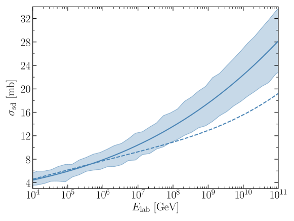
Figure 2: The growth of the single-diffractive cross section with lab energies up to $\sqrt{s}=10^{11}$ GeV for both the U-matrix unitarisation scheme (solid curve) and the eikonal (dashed curve). We show a $1\sigma$ error band in the U-matrix case. The corresponding band is similar in the eikonal case, but we omit it for clarity.

Despite their equivalence for existing data, the two schemes give significantly different predictions for the single-diffractive cross section at ultra-high energies. Unlike the total, elastic, and inelastic cross sections, the single diffractive cross section obtained using the eikonal scheme is noticeably different from that obtained using the U-matrix, with the former exhibiting a slower growth with energies than the latter, as shown in Fig. 2. This difference is especially significant for ongoing cosmic-ray experiments measuring the $pp$ cross-section at high energies from tens of TeV up to the GZK cut-off, $E_{\text{lab}}\approx 5\times 10^{10}$ GeV. As the single-diffraction is the parent process to forward pions, and hence to forward muons, it seems that considering different unitarisation schemes would lead to different muon multiplicities at ultra-high energies.

6 Conclusions

We have shown how the scheme proposed by Gotsman, Levin and Maor Gotsman:1999xq ; Gotsman:2014pwa could be adapted to other unitarisation schemes. We have also shown how the vertices of the mixed states could be deduced from those of the proton, allowing a more constrained parameterisation.

Using up-to-date collider data on $p\overset{\scriptscriptstyle\left(-\right)}{p}$ total, elastic, and single diffractive cross sections, including 13 TeV data from recent LHC experiments, we have determined best fits to the parameters governing these cross sections in the context of different unitarisation schemes. Specifically, we have shown that the U-matrix scheme fits the data as well as the more ubiquitous eikonal scheme. In fact, the fits have a slight preference for the U Matrix. This difference is driven by the single diffractive cross section, especially at high energies, while the best-fit total and elastic cross sections are nearly identical up to energies of 13 TeV when using either of these schemes.

A consequence of the indifference of the elastic cross section to the choice of the unitarisation scheme up to tens of TeV is that values of the $\rho$ parameter remain largely unaffected by the choice of the scheme too. We use our best-fit parameters to compute this parameter across different energies, and find that the corresponding values conform to existing data, to the exception of the TOTEM measurement at 13 TeV.

We have also analysed how the fits improve if one uses the generalised eikonal and U-matrix schemes and we find that these generalisations — at the cost of an additional free parameter ($\omega\text{ or }\omega^{\prime}$) — do not improve the fits significantly.

The upshot of our analysis is that the overall best-fit cross section, in light of up-to-date collider data, is obtained using amplitudes unitarised via the U-matrix scheme. The resulting $p\overset{\scriptscriptstyle\left(-\right)}{p}$ single diffractive cross section shows a sharper growth at high energies than does the one obtained using the more commonly used eikonal scheme, and unitarisation could have an impact on the description of ultra-high-energy cosmic-ray showers.

- (1) A. Donnachie and P.V. Landshoff, and total cross sections and elastic scattering, Phys. Lett. B727 (2013) 500 [1309.1292].
- (2) E. Gotsman, E. Levin and U. Maor, Diffractive dissociation and eikonalization in high-energy p p and p anti-p collisions, Phys.Rev.D 49 (1994) 4321 [hep-ph/9310257].
- (3) A. Shoshi, F. Steffen and H. Pirner, S matrix unitarity, impact parameter profiles, gluon saturation and high-energy scattering, Nucl.Phys.A 709 (2002) 131 [hep-ph/0202012].
- (4) O.V. Selyugin and J.R. Cudell, Saturation effects in pp scattering in the impact-parameter representation, Nucl. Phys. Proc. Suppl. 146 (2005) 185 [hep-ph/0412338].
- (5) J.R. Cudell, E. Predazzi and O.V. Selyugin, New analytic unitarisation schemes, Phys. Rev. D79 (2009) 034033 [0812.0735].
- (6) ALICE collaboration, Measurement of inelastic, single- and double-diffraction cross sections in proton–proton collisions at the LHC with ALICE, Eur. Phys. J. C73 (2013) 2456 [1208.4968].
- (7) ATLAS collaboration, Measurement of the total cross section from elastic scattering in pp collisions at TeV with the ATLAS detector, Nucl. Phys. B889 (2014) 486 [1408.5778].
- (8) ATLAS collaboration, Measurement of the total cross section from elastic scattering in collisions at TeV with the ATLAS detector, Phys. Lett. B761 (2016) 158 [1607.06605].
- (9) ATLAS collaboration, Measurement of the Inelastic Proton-Proton Cross-Section at TeV with the ATLAS Detector, Nature Commun. 2 (2011) 463 [1104.0326].
- (10) ATLAS collaboration, Inelastic proton cross section at 13 TeV with ATLAS, PoS ICHEP2016 (2017) 1127.
- (11) CMS collaboration, Measurement of the inelastic proton-proton cross section at TeV, JHEP 07 (2018) 161 [1802.02613].
- (12) LHCb collaboration, Measurement of the inelastic cross-section at a centre-of-mass energy of 13 TeV, JHEP 06 (2018) 100 [1803.10974].
- (13) TOTEM collaboration, First measurement of the total proton-proton cross section at the LHC energy of =7 TeV, EPL 96 (2011) 21002 [1110.1395].
- (14) TOTEM collaboration, Measurement of proton-proton elastic scattering and total cross-section at S**(1/2) = 7-TeV, EPL 101 (2013) 21002.
- (15) TOTEM collaboration, Luminosity-independent measurements of total, elastic and inelastic cross-sections at TeV, EPL 101 (2013) 21004.
- (16) TOTEM collaboration, Luminosity-Independent Measurement of the Proton-Proton Total Cross Section at TeV, Phys. Rev. Lett. 111 (2013) 012001.
- (17) TOTEM collaboration, First measurement of elastic, inelastic and total cross-section at TeV by TOTEM and overview of cross-section data at LHC energies, Eur. Phys. J. C79 (2019) 103 [1712.06153].
- (18) TOTEM collaboration, Measurement of proton-proton inelastic scattering cross-section at = 7 TeV, EPL 101 (2013) 21003.
- (19) UA4 collaboration, Measurement of the Proton - anti-Proton Total and Elastic Cross-Sections at the CERN SPS Collider, Phys. Lett. 147B (1984) 392.
- (20) UA5 collaboration, Antiproton-proton cross sections at 200 and 900 GeV c.m. energy, Z. Phys. C32 (1986) 153.
- (21) CDF collaboration, Measurement of small angle elastic scattering at GeV and 1800 GeV, Phys. Rev. D50 (1994) 5518.
- (22) E-710 collaboration, A Luminosity Independent Measurement of the Total Cross-section at .8-tev, Phys. Lett. B243 (1990) 158.
- (23) E710 collaboration, Elastic Scattering at = 1020-GeV, Nuovo Cim. A106 (1993) 123.
- (24) CDF collaboration, Measurement of single diffraction dissociation at GeV and 1800 GeV, Phys. Rev. D50 (1994) 5535.
- (25) E811 collaboration, A Measurement of the proton-antiproton total cross-section at = 1.8-TeV, Phys. Lett. B445 (1999) 419.
- (26) E-811 collaboration, The Ratio, , of the Real to the Imaginary Part of the Forward Elastic Scattering Amplitude at = 1.8-TeV, Phys. Lett. B537 (2002) 41.
- (27) F. Riehn, R. Engel, A. Fedynitch, T.K. Gaisser and T. Stanev, Hadronic interaction model Sibyll 2.3d and extensive air showers, Phys. Rev. D 102 (2020) 063002 [1912.03300].
- (28) S. Ostapchenko, QGSJET-III model: physics and preliminary results, EPJ Web Conf. 208 (2019) 11001.
- (29) L. Anchordoqui, M.T. Dova, A.G. Mariazzi, T. McCauley, T.C. Paul, S. Reucroft et al., High energy physics in the atmosphere: Phenomenology of cosmic ray air showers, Annals Phys. 314 (2004) 145 [hep-ph/0407020].
- (30) Pierre Auger collaboration, The Pierre Auger Cosmic Ray Observatory, Nucl. Instrum. Meth. A798 (2015) 172 [1502.01323].
- (31) Telescope Array collaboration, Telescope array experiment, Nucl. Phys. Proc. Suppl. 175-176 (2008) 221.
- (32) IceCube collaboration, IceTop: The surface component of IceCube, Nucl. Instrum. Meth. A700 (2013) 188 [1207.6326].
- (33) A. Bhattacharya, J.-R. Cudell, R. Oueslati and A. Vanthieghem, The proton inelastic cross section at ultrahigh energies, 2012.07970.
- (34) M.L. Good and W.D. Walker, Diffraction disssociation of beam particles, Phys. Rev. 120 (1960) 1857.
- (35) J.R. Cudell, A. Lengyel and E. Martynov, The Soft and the hard pomerons in hadron elastic scattering at small , Phys. Rev. D73 (2006) 034008 [hep-ph/0511073].
- (36) J. Cudell and O.V. Selyugin, Saturation regimes at lhc energies, in Proceedings, 4th Symposium on LHC Physics and Detectors: Batavia, USA, May 1-3, 2003, vol. 54, pp. A441–A444, 2004 [hep-ph/0309194].
- (37) A. Logunov, V. Savrin, N. Tyurin and O. Khrustalev, Equal-time equation for two-particle system in quantum field theory, Teor.Mat.Fiz. 6 (1971) 157.
- (38) V. Savrin, N. Tyurin and O. Khrustalev, The u matrix method in the theory of strong interactions, Fiz.Elem.Chast.Atom.Yadra 7 (1976) 21.
- (39) UA5 collaboration, UA5: A general study of proton-antiproton physics at = 546-GeV, Phys. Rept. 154 (1987) 247.
- (40) E710 collaboration, Diffraction dissociation in collisions at = 1.8-TeV, Phys. Lett. B301 (1993) 313.
- (41) A. Donnachie and P.V. Landshoff, Soft diffraction dissociation, hep-ph/0305246.
- (42) E. Gotsman, E. Levin and U. Maor, The Survival probability of large rapidity gaps in a three channel model, Phys. Rev. D60 (1999) 094011 [hep-ph/9902294].
- (43) Pierre Auger collaboration, Measurement of the fluctuations in the number of muons in extensive air showers with the Pierre Auger Observatory, 2102.07797.
- (44) E. Gotsman, E. Levin and U. Maor, A comprehensive model of soft interactions in the LHC era, Int. J. Mod. Phys. A30 (2015) 1542005 [1403.4531].
- (45) V.A. Khoze, A.D. Martin and M.G. Ryskin, Diffraction at the LHC, European Physical Journal C 73 (2013) 2503 [1306.2149].
- (46) V.A. Khoze, A.D. Martin and M.G. Ryskin, Elastic and diffractive scattering at the LHC, Phys. Lett. B784 (2018) 192 [1806.05970].
- (47) V.A. Khoze, A.D. Martin and M.G. Ryskin, Multiple interactions and rapidity gap survival, Journal of Physics G Nuclear Physics 45 (2018) 053002 [1710.11505].
- (48) Particle Data Group collaboration, Review of Particle Physics, Phys. Rev. D98 (2018) 030001.
- (49) A. Fedynitch, F. Riehn, R. Engel, T.K. Gaisser and T. Stanev, Hadronic interaction model sibyll 2.3c and inclusive lepton fluxes, Phys. Rev. D100 (2019) 103018 [1806.04140].
- (50) S. Ostapchenko, Monte Carlo treatment of hadronic interactions in enhanced Pomeron scheme: I. QGSJET-II model, Phys. Rev. D83 (2011) 014018 [1010.1869].
- (51) J.R. Cudell, K. Kang and S.K. Kim, Simple pole fits to p p and anti-p p total cross-sections and real parts, Phys. Lett. B 395 (1997) 311 [hep-ph/9601336].
- (52) M.M. Block, Sifting data in the real world, Nucl. Instrum. Meth. A 556 (2006) 308 [physics/0506010].
- (53) UA5 collaboration, Diffraction Dissociation at the CERN Pulsed Collider at CM Energies of 900-GeV and 200-GeV, Z. Phys. C33 (1986) 175.
- (54) CDF collaboration, Double Diffraction Dissociation at the Fermilab Tevatron Collider, Phys. Rev. Lett. 87 (2001) 141802 [hep-ex/0107070].
- (55) A. Donnachie and P.V. Landshoff, Small elastic scattering and the parameter, Phys. Lett. B798 (2019) 135008 [1904.11218].
- (56) TOTEM collaboration, First determination of the parameter at TeV: probing the existence of a colourless C-odd three-gluon compound state, Eur. Phys. J. C79 (2019) 785 [1812.04732].
- (57) J.R. Cudell and O.V. Selyugin, TOTEM data and the real part of the hadron elastic amplitude at 13 TeV, 1901.05863.